Adomian Decomposition Based Numerical Scheme for Flow simulationsJournal: Numerical Methods for Partial Differential Equations

Imanol Garcia-Beristain Email: igarcia@bcamath.org Corresponding author: Corresponding author: Tel.:+34 946 567 842 Address: BCAM - Basque Center for Applied Mathematics, Alameda Mazarredo 14, 48009, Bilbao, Spain Lakhdar Remaki Address: BCAM - Basque Center for Applied Mathematics, Alameda Mazarredo 14, 48009, Bilbao, Spain Address: Department of Mathematics and Computer Science, Alfaisal University, KSA

Abstract

This paper proposes a numerical method based on the Adomian decomposition approach for the time discretization, applied to Euler equations. A recursive property is demonstrated that allows to formulate the method in an appropriate and efficient way. To obtain a fully numerical scheme, the space discretization is achieved using the classical DG techniques. The efficiency of the obtained numerical scheme is demonstrated through numerical tests by comparison to exact solution and the popular Runge-Kutta DG method results.

Keywords:

Adomian decomposition, Euler equations, Linearized Euler Equations, Aeroacoustics, Discontinuous Galerkin (DG)

I Introduction

Linearized Euler equations (LEE) are extensively used in many problems modeling and simulation. In particular simulating wave propagation in aeroacoustic field. These equations offer, on one hand, the advantage to be faster than solving the nonlinear Euler equations since large domains are required for propagation. On the other hand, the information about the mean flow is preserved comparing to a simple wave equation. This is due to the fact that the linearization is achieved around a mean flow. Many aeroacoustic applications are of big importance for industry and for human life quality improvement. For instance, noise reduction in transportation. Especially, with the sensitive population’s mobility growth thanks to the development of fast transportation facilities. In the US, the Joint Planning and Development Office (JPDO) is planning a new NextGen system that increases the air traffic by a factor of 3 towards 2025. Therefore reducing harmful sound effects becomes critical in order to achieve this goal because the JPDO indicates that without this substantial effort the number of people exposed to very high levels of noise will increase substantially.

The LEE equations are numerically solved using different methods including finite volume, finite elements, discontinuous Galerkin and spectral methods. Research is still actively ongoing to design more effective numerical schemes suitable for the large scales required by the practical problems.

In this paper we propose an accurate and cost-effective numerical scheme based on the semi-analytical Adomian decomposition method, proposed by Adomian [45, 46, adm3], and used by many authors to solve a big range of problems ranging from linear or nonlinear equations for deterministic or stochastic PDEs. It seems to be a promising trend in the field of PDEs solution approximation. See for instance the important work of Wazwaz [48, 49, 50, 51, 52], and other relevant articles [55, 56, 57]. The reader is especially referred to the nice review paper on the topic [49].

To derive the proposed approach, the semi-analytical Adomian decomposition technique is applied to the Euler equations. Then, a recursive property for the obtained time scheme is proved. This allows to formulate the method in a simple and practical form, easy to implement and cost-effective. To fully derive the numerical scheme (including space discretization) the classical discontinuous Galerkin (DG) approach is used. We refer to the obtained time scheme by ABS standing for Adomian Based Schemes and ABS-DG when the space discretization is achieved using discontinuous Galerkin method. To demonstrate the ABS-DG effectiveness, the (DG) method is implemented, numerical tests performed, and results compared. Results are also compared to exact solutions when available.

In sections 2 a short overview on the Adomian decomposition method and the Euler nonlinear and linearized equations are given. In sections 3 details of the proposed ABS and ABS-DG schemes are provided. In section 4 a connection between the ABS and Runge-Kutta (RK) methods is established for the linear case. Tests are performed and reported in section 5, while conclusions are drawn in section 6.

II Review

In this section a short review on the Adomian decomposition method and nonlinear and linearized Euler equations are given.

II.I The Adomian Decomposition Method

In the following, a short description of the Adomian decomposition method is given. For more details we refer to [45, 46, adm3, 49]. The first step of the method consists in identifying the differential equations in the following form,

L(u)+R(u)+N(u)=0

(1)

Where $L$ and $R$ are the linear part of the differential operator, with $L$ being the part that is easily invertible. $N$ is the nonlinear part.

Note that it is not necessary to distinguish the non invertible linear part from the nonlinear invertible one. Both can be represented by the sum $N+R$ by a single operator, $N$ .

Adomian algorithm considers the solution $u$ as a summation over a series,

u=\sum_{n=0}^{\infty}u_{n}.

(2)

While operator $N$ is given by the expansion of the Adomian polynomials, $N_{n}$ .

N=\sum_{n=0}^{\infty}N_{n}.

(3)

where the Adomian polynomial coefficients $N_{n}$ are given by

N_{n}=\frac{1}{n!}\frac{\partial^{n}}{\partial\lambda^{n}}\left[N\left(\sum_{k=0}^{n}\lambda^{k}u_{k}\right)\right]_{\lambda=0}.

(4)

Finally, $u_{n}$ terms are computed as

u_{n+1}=L^{-1}(N_{n})

(5)

II.II The non-conservative Euler equations

The two-dimensional compressible inviscid flow equations are given by the Euler equations. Formulated relative to a Cartesian $(x,y)$ coordinate system, and in a primitive variable form as

\left\{\begin{array}[]{lr}\frac{\partial\rho}{\partial t}+\partial_{x}(\rho u)+\partial_{y}(\rho v)=0\\ \frac{\partial u}{\partial t}+u\partial_{x}(u)+v\partial_{y}(u)+\frac{1}{\rho}\partial_{x}p=0\\ \frac{\partial v}{\partial t}+u\partial_{x}(v)+v\partial_{y}(v)+\frac{1}{\rho}\partial_{y}p=0\\ \frac{\partial p}{\partial t}+u\partial_{x}(p)+v\partial_{y}(p)+\gamma p(\partial_{x}(u)+\partial_{y}(v))=0\\ \end{array}\right.

(6)

where $\rho$ and $p$ denote the averaged density and pressure of the fluid respectively and $E=e+\frac{1}{2}(u_{\alpha}u_{\alpha})$ is the total energy per unit mass, with $e$ being the internal energy per unit mass. $u_{\alpha}$ is the averaged velocity of the fluid in direction $x_{\alpha}$ and $\delta_{\alpha i}$ is the Kronecker delta.

The equation set is closed with the addition of the ideal gas state equation. i.e. $p=\rho(\gamma-1)e$ , where $\rho$ is the density and $\gamma$ is the ratio of specific heats. Solutions to the resulting set of equations are defined on a fixed spatial computational domain $\Omega$ .

Euler equations can also be written in vector or matrix form,

\frac{\partial Q}{\partial t}+\mathcal{A}\frac{\partial Q}{\partial x}+\mathcal{B}\frac{\partial Q^{\prime}}{\partial y}=S.

(7)

Where, $Q(x,y,t)=(\rho,u_{1},u_{2},p)^{t}$ and

\displaystyle\mathcal{A}(x,y,t)=\begin{pmatrix}u&\rho&0&0\\ 0&u&0&1/\rho\\ 0&0&u&0\\ 0&\rho c^{2}&0&u\\ \end{pmatrix}

\displaystyle\mathcal{B}(x,y,t)=\begin{pmatrix}v&0&\rho&0\\ 0&v&0&0\\ 0&0&v&1/\rho\\ 0&0&\rho c^{2}&v\\ \end{pmatrix}.

II.III The Linearized Euler Equations

LEE system is obtained after a linearization around a mean flow. This is achieved by assuming solution is composed of a mean and a perturbation part: $Q(x,y,t)=Q_{0}(x,y,t)+Q^{\prime}(x,y,t)$ (and also for the source term). Additionally, the mean flow values are assumed to satisfy

\displaystyle\frac{\partial Q_{0}}{\partial t}+\mathcal{A}_{0}\frac{\partial Q_{0}}{\partial x}+\mathcal{B}_{0}\frac{\partial Q_{0}}{\partial y}=S_{0}.

(8)

Inserting previous equations into the Euler system, and performing nondimensionalization, it yields [64],

\frac{\partial Q^{\prime}}{\partial t}+\mathcal{A}_{0}\frac{\partial Q^{\prime}}{\partial x}+\mathcal{B}_{0}\frac{\partial Q^{\prime}}{\partial y}+\mathcal{A}^{\prime}\dfrac{\partial Q_{0}}{\partial x}+\mathcal{B}^{\prime}\dfrac{\partial Q_{0}}{\partial y}=S^{\prime}.

(9)

Where $Q^{\prime}=\left(\rho^{\prime},u^{\prime},v^{\prime},p^{\prime}\right)^{t}$ and

\displaystyle\mathcal{A}_{0}(x,y,t)=\begin{pmatrix}M_{1}&1&0&0\\ 0&M_{1}&0&1\\ 0&0&M_{1}&0\\ 0&1&0&M_{1}\\ \end{pmatrix}

\displaystyle\mathcal{B}_{0}(x,y,t)=\begin{pmatrix}M_{2}&0&1&0\\ 0&M_{2}&0&0\\ 0&0&M_{2}&1\\ 0&0&1&M_{2}\\ \end{pmatrix}.

Subscript $0$ in matrices $\mathcal{A}_{0},\mathcal{B}_{0}$ , denotes exclusive dependency to mean flow values. Whereas primes in $\mathcal{A}^{\prime}$ and $\mathcal{B}^{\prime}$ denote evaluation with perturbed variables. Those last perturbation matrices can be considered negligible if mean flow spatial derivatives are moderated,

\displaystyle\mathcal{A}^{\prime}\dfrac{\partial Q}{\partial x}=0

\displaystyle\mathcal{B}^{\prime}\dfrac{\partial Q}{\partial y}=0

(10)

Finally, no source terms will be assumed $S=S^{\prime}=0$ .

In this paper time independent and constant in space mean values are considered for simplicity. Therefore, $\mathcal{A}_{0}$ and $\mathcal{B}_{0}$ matrices are constant. Nonetheless, one could consider space dependent matrices without lost of generality.

In summary, the following governing equations are yielded

\frac{\partial Q^{\prime}}{\partial t}+\mathcal{A}_{0}\frac{\partial Q^{\prime}}{\partial x}+\mathcal{B}_{0}\frac{\partial Q^{\prime}}{\partial y}=0

(11)

For convenience we drop prime symbol from $Q^{\prime}$ .

III Adomian Based Schemes (ABS)

In this paper we propose a cost-effective numerical scheme to solve LEE (eq. 11). Method is based on the Adomian decomposition technique for time discretization, and DG techniques (which can be replaced by other techniques) for the space discretization. The scheme is assessed by comparison to Runge-Kutta DG method, and exact solutions. The DG space discretization is implemented following the approach proposed by Shu [65]. For other classical DG discretization options, the reader is pointed to Cockburns paper [66]. Details are not provided in this paper since it is a well-known method. However, the application of Adomian decomposition for time discretization is described in detail, since it is the main contribution of the paper.

III.I The ABS Scheme Derivation

Even if the proposed ABS scheme is applied and assessed for the LEE, the scheme is derived for the general case of nonlinear Euler equations. This is motivated by the fact that some useful properties simplify the scheme formulation for both LEE and the nonlinear case.

To apply the Adomian decomposition technique described in section II.I to Euler equations (6), we propose to set

$L=\frac{\partial}{\partial t}$ and then $L^{-1}=\int_{0}^{t}$

Referring by $F_{x}$ and $F_{y}$ to the $x$ and $y$ space derivatives, operator $N$ is given by

$N(Q)=F_{x}(Q)+F_{y}(Q)$

with $Q$ being the primitive variables

\displaystyle Q(x,y)=\begin{pmatrix}\rho\\ u\\ v\\ p\end{pmatrix}.

(12)

Applying decomposition from (2), in vector notation,

\displaystyle Q=\sum_{k=0}^{\infty}Q_{k},

(13)

The Adomian coefficients from (3) can be written as

N_{n}(x,y,t)=\frac{1}{n!}\frac{\partial^{n}}{\partial\lambda^{n}}\left[F_{x}\left(\sum_{k=0}^{n}\lambda^{k}Q_{k}\right)+F_{y}\left(\sum_{k=0}^{n}\lambda^{k}Q_{k}\right)\right]_{\lambda=0}.

(14)

Therefore, substituting into the governing equations,

\displaystyle N_{n}(x,y,t)==\frac{1}{n!}\frac{\partial^{n}}{\partial\lambda^{n}}\left[\begin{array}[]{l}\partial_{x}\left((\sum_{k=0}^{n}\lambda^{k}\rho_{k})(\sum_{k=0}^{n}\lambda^{k}u_{k})\right)\\[-5.0pt] \hskip 28.45274pt+\partial_{y}\left((\sum_{k=0}^{n}\lambda^{k}\rho_{k})(\sum_{k=0}^{n}\lambda^{k}v_{k})\right)=0\\[10.0pt] (\sum_{k=0}^{n}\lambda^{k}u_{k})\partial_{x}(\sum_{k=0}^{n}\lambda^{k}u_{k})+(\sum_{k=0}^{n}\lambda^{k}v_{k})\partial_{y}(\sum_{k=0}^{n}\lambda^{k}u_{k})+\\[-2.0pt] \hskip 28.45274pt\left(\dfrac{1}{\sum_{k=0}^{n}\lambda^{k}{\rho}_{k}}\right)\partial_{x}\left(\sum_{k=0}^{n}\lambda^{k}p_{k}\right)=0\\[10.0pt] (\sum_{k=0}^{n}\lambda^{k}u_{k})\partial_{x}(\sum_{k=0}^{n}\lambda^{k}v_{k})+(\sum_{k=0}^{n}\lambda^{k}v_{k})\partial_{y}(\sum_{k=0}^{n}\lambda^{k}v_{k})+\\[-2.0pt] \hskip 28.45274pt\left(\dfrac{1}{\sum_{k=0}^{n}\lambda^{k}{\rho}_{k}}\right)\partial_{y}\left(\sum_{k=0}^{n}\lambda^{k}p_{k}\right)=0\\[10.0pt] (\sum_{k=0}^{n}\lambda^{k}u_{k})\partial_{x}(\sum_{k=0}^{n}\lambda^{k}p_{k})+(\sum_{k=0}^{n}\lambda^{k}v_{k})\partial_{y}(\sum_{k=0}^{n}\lambda^{k}p_{k})+\\[-5.0pt] \hskip 28.45274pt\gamma(\sum_{k=0}^{n}\lambda^{k}p_{k})\left(\partial_{x}(\sum_{k=0}^{n}\lambda^{k}p_{k})+\partial_{y}(\sum_{k=0}^{n}\lambda^{k}v_{k})\right)=0\end{array}\right]_{\lambda=0}.

And $Q_{n+1}$ terms are computed recursively by (5),

Q_{n+1}(x,y,t)=\int_{0}^{t}N_{n}(x,y,t).

(23)

Let’s expand each equation of the vector $N_{n}=(A_{n},B_{n},C_{n},D_{n})^{t}$ , corresponding each component to an equation of the Euler system. We will first derive the term $A_{n}$ corresponding to the continuity equation. Then $B_{n},C_{n},D_{n}$ will be obtained in a similar way.

From formula (III.I) $A_{n}$ is given by:

\displaystyle A_{n}(x,y,t)=\frac{1}{n!}\frac{\partial^{n}}{\partial\lambda^{n}}\left[\frac{\partial}{\partial x}\left((\sum_{k=0}^{n}\lambda^{k}\rho_{k})(\sum_{k=0}^{n}\lambda^{k}u_{k})\right)+\frac{\partial}{\partial y}\left((\sum_{k=0}^{n}\lambda^{k}\rho_{k})(\sum_{k=0}^{n}\lambda^{k}v_{k})\right)\right]_{\lambda=0}

Let’s develop the first term in the summation. First, the derivative order is exchanged. Meaning,

\displaystyle\frac{1}{n!}\frac{\partial^{n}}{\partial\lambda^{n}}\left[\frac{\partial}{\partial x}\left(\cdot\right)\right]_{\lambda=0}=\frac{1}{n!}\frac{\partial}{\partial x}\left[\frac{\partial^{n}}{\partial\lambda^{n}}\left(\cdot\right)\right]_{\lambda=0}.

Using the Leibniz formula, we get

\displaystyle\frac{\partial^{n}}{\partial\lambda^{n}}\left(\sum_{k=0}^{n}\lambda^{k}\rho_{k}\sum_{k=0}^{n}\lambda^{k}u_{k}\right)

\displaystyle=\sum_{j=0}^{n}\binom{j}{k}\frac{\partial^{n-j}}{\partial\lambda^{n-j}}\left(\sum_{k=0}^{n}\lambda^{k}\rho_{k}\right)\frac{\partial^{j}}{\partial\lambda^{j}}\left(\sum_{k=0}^{n}\lambda^{k}u_{k}\right)

with

		$\displaystyle\frac{\partial^{n-j}}{\partial\lambda^{n-j}}\left(\sum_{k=0}^{n}\lambda^{k}\rho_{k}\right)\|_{\lambda=0}=(n-j)!\,\rho_{n-j}$	$\displaystyle\binom{j}{k}=\dfrac{n!}{j!\ (n-j)!}$
		$\displaystyle\frac{\partial^{j}}{\partial\lambda^{j}}\left(\sum_{k=0}^{n}\lambda^{k}u_{k}\right)\|_{\lambda=0}=(j)!\,u_{j}$

Then

\displaystyle\frac{1}{n!}\frac{\partial}{\partial x}\left[\frac{\partial^{n}}{\partial\lambda^{n}}\left((\sum_{k=0}^{n}\lambda^{k}\rho_{k})(\sum_{k=0}^{n}\lambda^{k}u_{k})\right)\right]_{\lambda=0}=\sum_{j=0}^{n}\frac{\partial}{\partial x}(\rho_{n-j}u_{j})

(24)

Similarly, for the second summation term we have,

\displaystyle\frac{1}{n!}\frac{\partial}{\partial y}\left[\frac{\partial^{n}}{\partial\lambda^{n}}\left((\sum_{k=0}^{n}\lambda^{k}\rho_{k})(\sum_{k=0}^{n}\lambda^{k}v_{k})\right)\right]_{\lambda=0}=\sum_{j=0}^{n}\frac{\partial}{\partial y}(\rho_{n-j}v_{j}).

(25)

Substituting both equations (24 - 25) into $A_{n}$ equation, we get the final formula

\displaystyle A_{n}=-\sum_{j=0}^{n}(\partial_{x}(\rho_{n-j}u_{j})+\partial_{y}(\rho_{n-j}v_{j}))

(26)

We obtain a similar formula for $D_{n}$ .

For $B_{n}$ and $C_{n}$ , first develop $\frac{1}{\sum_{k=0}^{n}\lambda^{k}\rho_{k}}$ as power series (note that $\lambda$ can be considered close to zero since we are concerned by the limit)

$\frac{1}{\sum_{k=0}^{n}\lambda^{k}\rho_{k}}=\sum_{k=0}^{\infty}\lambda^{k}\widehat{\rho}_{k}$

That is,

	$\displaystyle 1$	$\displaystyle=(\sum_{k=0}^{n}\lambda^{k}\rho_{k})(\sum_{k=0}^{\infty}\lambda^{k}\widehat{\rho}_{k})$
		$\displaystyle=\rho_{0}\widehat{\rho}_{0}+\sum_{k=1}^{\infty}(\sum_{j=0}^{k}\rho_{j}\widehat{\rho}_{k-j})\lambda^{k}$

Then we obtain the flowing recursive formula

\displaystyle\left\{\begin{array}[]{lr}\widehat{\rho}_{0}=\frac{-1}{\rho_{0}}\\ \widehat{\rho}_{k}=\frac{-1}{\rho_{0}}\sum_{j=1}^{k}\rho_{j}\widehat{\rho}_{k-j},\qquad\text{for}\ k=1,\ldots,\infty\end{array}\right.

such that we can perform a change of variable in system (III.I) and set,

$\left(\dfrac{1}{\sum_{k=0}^{n}\lambda^{k}{\rho}_{k}}\right)\partial_{x}\left(\sum_{k=0}^{n}\lambda^{k}p_{k}\right)=\left(\lambda^{k}\hat{\rho}_{k}\right)\partial_{x}\left(\sum_{k=0}^{n}\lambda^{k}p_{k}\right)$

And therefore using the same simplifications as for $A_{n}$ , we finally obtain the following formula for $N_{n}$

N_{n}(x,y,t)=\left\{\begin{array}[]{lr}A_{n}=-\sum_{j=0}^{n}(\partial_{x}(\rho_{n-j}u_{j})+\partial_{y}(\rho_{n-j}v_{j}))\\ B_{n}=-\sum_{j=0}^{n}(u_{n-j}\partial_{x}u_{j}+v_{n-j}\partial_{y}u_{j}+\widehat{\rho}_{n-j}\partial_{x}p_{j})\\ C_{n}=-\sum_{j=0}^{n}(u_{n-j}\partial_{x}v_{j}+v_{n-j}\partial_{y}v_{j}+\widehat{\rho}_{n-j}\partial_{y}p_{j})\\ D_{n}=-\sum_{j=0}^{n}(u_{n-j}\partial_{x}p_{j}+v_{n-j}\partial_{y}p_{j}+\gamma p_{j}(\partial_{x}u_{n-j}+\partial_{y}v_{n-j}))\\ \end{array}\right.

(29)

In practice, time integration (23) is in general not easy to compute, or at least in a very accurate way. Indeed, Adomian series coefficients are polynomials in time whose computed coefficients need to be stored. The following Theorem remedy to this problem and allows a systematic and exact time integration by a simple multiplication by time $t$ .

Theorem: In formula (29) the expression of $N_{n}$ can be expressed as

N_{n}(x,y,t)=t^{n}\overline{N}_{n}(x,y)

(30)

Where $\overline{N}_{n}(x,y)$ , is an expression depending only on $x$ and $y$

Proof: We establish the proof by induction. We will do it only for the first momentum equation terms ( $B_{n}$ ) and the others are obtained in a similar way.

Note that if equation (30) is fulfilled, a similar relation is hold by field variables,

Q_{n+1}(x,y,t)=\int_{0}^{t}N_{n}(x,y,t)dt=\frac{t^{n+1}}{(n+1)}\overline{N}_{n}(x,y)=t^{n+1}\overline{Q}_{n}(x,y).

(31)

Note also that in the recursive formula of $\widehat{\rho}_{k}$ the sum of the indexes is always equal to $k$ , this implies that $\widehat{\rho}_{k}$ satisfies the formula 30 as long as $\rho_{k}$ satisfies it.

\widehat{\rho}_{k}(x,y,t)=t^{k}\widehat{\overline{\rho}}_{k}(x,y)

(32)

Now to initialize the recursive proof, let’s verify the relation for $B_{o}$ and $B_{1}$ . From (29) We have

$B_{0}(x,y,t)=-(u_{0}\partial_{x}u_{0}+v_{0}\partial_{x}u_{0}+\frac{1}{\rho_{0}}\partial_{x}p_{0})=t^{0}\overline{B}_{0}(x,y)$ .

Then a new state variable term is computed with (29),

Q_{1}(x,y,t)=\int_{0}^{t}N_{0}(x,y)=tN_{0}(x,y).

(33)

And therefore a new Adomian polynomial,

$B_{1}=-(u_{1}\partial_{x}u_{0}+v_{1}\partial_{x}u_{0}+\widehat{\rho}_{1}\partial_{x}p_{0}+u_{0}\partial_{x}u_{1}+v_{0}\partial_{x}u_{1}+\widehat{\rho}_{0}\partial_{x}p_{1})$

Recall from (32),

$\widehat{\rho}_{1}=t\widehat{\overline{\rho}}_{1}(x,y)$

Substituting $\widehat{\rho}_{1}$ and $Q_{1}$ into the expression of $B_{1}$ , it is easy to verify that $B_{1}(x,y,t)=t\overline{B}_{1}(x,y)$

Now assume relation (30) is valid till index $n$ and lets proof it for $n+1$ . We proceed exactly as for $N_{1}$ , since the relation is valid for order $n$ we have

$N_{n}(x,y,t)=t^{n}\overline{N}_{n}(x,y)$

Then,

Q_{n+1}(x,y,t)=\int_{0}^{t}N_{n}(x,y,t)=\frac{t^{n+1}}{n+1}\overline{N}_{n}(x,y)=t^{n+1}\overline{Q}_{n}(x,y)

(34)

By substituting this expression in equation (29) we obtain for the first momentum $B_{n+1}$ .

	$\displaystyle B_{n+1}$	$\displaystyle=\sum_{j=0}^{n}u_{n+1-j}\partial_{x}u_{j}+v_{n+1-j}\partial_{y}u_{j}+\widehat{\rho}_{n+1-j}\partial_{x}p_{j}$
		$\displaystyle=\sum_{j=0}^{n}\left[\left(t^{n+1-j}\overline{u}_{n-j}(x,y)\right)\left(\partial_{x}t^{j}\overline{u}_{j-1}(x,y)\right)+\left(t^{n+1-j}\overline{v}_{n-j}(x,y)\right)\left(\partial_{y}t^{j}\overline{u}_{j-1}(x,y)\right)\right.$
		$\displaystyle\left.\hskip 28.45274pt+\left(t^{n+1-j}\widehat{{\rho}}_{n+1-j}\right)\left(\partial_{x}t^{j}\overline{p}_{j-1}(x,y)\right)\right]$
		$\displaystyle=\sum_{j=0}^{n}t^{n+1}\left[\overline{u}_{n-j}(x,y)\partial_{x}\overline{u}_{j-1}(x,y)+\overline{v}_{n-j}(x,y)\partial_{y}\overline{u}_{j-1}(x,y)+\widehat{{\rho}}_{n+1-j}\partial_{x}\overline{p}_{j-1}(x,y)\right]$

Which gives,

B_{n+1}=-t^{n+1}\sum_{j=0}^{n}\left[\overline{u}_{n-j}(x,y)\partial_{x}\overline{u}_{j-1}(x,y)+\overline{v}_{n-j}(x,y)\partial_{y}\overline{u}_{j-1}(x,y)+\widehat{{\rho}}_{n+1-j}\partial_{x}\overline{p}_{j-1}(x,y)\right]

This is a monomial of degree $n+1$ in time with a coefficient depending only on $x,y$ , therefore $B_{n+1}$ can be written as

$B_{n+1}(t,x,y)=t^{n+1}\overline{B}_{n}(x,y)$

Which achieves the proof of the Theorem.

∎

III.II The ABS formula

Using equation (34) we can derive a formula for $Q_{n+1}$ that doesn’t require any time integration,

$\displaystyle Q_{n+1}(x,y,t)$	$\displaystyle=\int_{0}^{t}{N_{n}(t,x,y)dt}=\int_{0}^{t}{t^{n}\overline{N}_{n}(x,y)dt}$
	$\displaystyle=\frac{t^{n+1}}{n+1}\overline{N}_{n}(x,y)=\frac{t}{n+1}\left[t^{n}\overline{N}_{n}(x,y)\right]$
	$\displaystyle=\frac{t}{n+1}N_{n}(t,x,y)$	(35)

Substituting the expression of $N_{n}$ we obtain

Q_{n+1}(x,y,t)=\left\{\begin{array}[]{lr}\frac{-t}{n+1}\left[\sum_{j=0}^{n}(\partial_{x}(\rho_{n-j}u_{j})+\partial_{y}(\rho_{n-j}v_{j}))\right]\\ \frac{-t}{n+1}\left[\sum_{j=0}^{n}(u_{n-j}\partial_{x}u_{j}+v_{n-j}\partial_{y}u_{j}+\widehat{\rho}_{n-j}\partial_{x}p_{j})\right]\\ \frac{-t}{n+1}\left[\sum_{j=0}^{n}(u_{n-j}\partial_{x}v_{j}+v_{n-j}\partial_{y}v_{j}+\widehat{\rho}_{n-j}\partial_{y}p_{j})\right]\\ \frac{-t}{n+1}\left[\sum_{j=0}^{n}(u_{n-j}\partial_{x}p_{j}+v_{n-j}\partial_{y}p_{j}+\gamma(\partial_{x}u_{n-j}+\partial_{y}v_{n-j})p_{j})\right]\\ \end{array}\right.

(36)

As it can be seen, once $\{Q_{1},\ldots,Q_{n}\}$ are calculated $Q_{n+1}$ is obtained without any time integration.

Considering space derivatives, the recursive formulation can lead to a fully analytical formulation, only depending on the initial condition. In literature some articles can be found where Mathematica is used to directly obtain an analytical solution to a simple initial condition (see for example [49, 53]). Nevertheless, using symbolic software to obtain a real problem solution can be very expensive in terms of computational cost, assuming it is possible to find an analytical expression for the initial condition problem. Moreover, calculating the derivatives in strong sense requires the initial condition to be smooth enough.

We hereby propose considering space derivatives in the weak sense and estimate them numerically. Although any numerical method can be used, in this work space derivatives are estimated using discontinuous Galerkin (DG) method as proposed by Shu [65]. However, different DG methods can be found in, for instance, Cockburn [66]. We refer to the obtained (fully discretized) scheme by ABS-DG.

Now and as mentioned in the introduction, detailed formulation of the ABS-DG scheme will be given for LEE, as it is our target application to assess the ABS-DG.

III.III The ABS-DG for LEE

For the LEE case, formula (36) is simplified to

Q_{n+1}(x,y,t)=\frac{-t}{n+1}\left[\mathcal{A}_{0}(x,y)\frac{\partial}{\partial x}Q_{n}(x,y,t)+\mathcal{B}_{0}(x,y)\frac{\partial}{\partial y}Q_{n}(x,y,t)\right]

III.IV Space discretization

Space discretization is achieved by applying the DG method for each term of the ABS series. The procedure is given in [65]. However, details for order zero DG is given here, which corresponds to a finite volume scheme, since results are used in next step for stability analysis.

In that case each $Q_{n}$ term is approximated at the cell center by

\displaystyle Q_{n}(x_{i},y_{i},t)\simeq\frac{1}{\mid S_{i}\mid}\int_{S_{i}}Q_{n}(x,y,t)\,\text{d}S,

where $S_{i}$ is a given cell surface (for a two-dimensional domain). This leads to

		$\displaystyle Q_{n+1}(x_{i},y_{i},t)=\frac{-t}{n+1}\frac{1}{\mid S_{i}\mid}\int_{\partial S_{i}}\Big[{\mathcal{A}_{0}}\ Q_{n}(x,y,t)\ \eta_{x}$
		$\displaystyle\hskip 159.3356pt+{\mathcal{B}_{0}}\ Q_{n}(x,y,t)\ \eta_{y}\Big]\ \text{d}S$
		$\displaystyle Q^{N}=\sum_{n=0}^{N}Q_{n}$

Here $Q^{N}$ is the approximated solution, and $N$ corresponds to the index for which $|Q_{N}|$ is smaller than a given tolerance.

Approximating fluxes as in the classical finite volume, we obtain the following ABS-DG zero order numerical scheme,

(ABS-DG)\left\{Q_{0}(x_{i},y_{i})=Q(x_{i},y_{i},0)~~\\ Q_{n+1}(x_{i},y_{i},t)=\frac{-t}{n+1}\frac{1}{\mid S_{i}\mid}\sum_{j}F_{n}^{i,j}~~\\ Q^{N}=\sum_{n=0}^{N}Q_{n}~~\right..

The numerical flux could be the Lax-Friedrichs flux approximation,

	$\displaystyle\begin{aligned} F^{i,j}_{n}=\dfrac{1}{2}\Big(\overline{\mathcal{A}}\left(Q_{n}^{i}+Q_{n}^{j}\right)\eta_{x}\ +\overline{\mathcal{B}}\left(Q_{n}^{i}+Q_{n}^{j}\right)\eta_{y}\Big)-\dfrac{1}{2}\alpha\Big(\left(Q_{n}^{j}-Q_{n}^{i}\right)\eta_{x}+\left(Q_{n}^{j}-Q_{n}^{i}\right)\eta_{y}\Big)\end{aligned}$		(37)
	$\displaystyle\begin{aligned} &\overline{\mathcal{A}}=\dfrac{\mathcal{A}^{i}+\mathcal{A}^{j}}{2}&\overline{\mathcal{B}}=\dfrac{\mathcal{B}^{i}+\mathcal{B}^{j}}{2}&\end{aligned}$		(38)

or any other suitable one.

III.V Stability Analysis

We study stability for the one-dimensional linear wave propagation equation,

\displaystyle\dfrac{\partial u}{\partial t}+a\dfrac{\partial u}{\partial x}=0,

(39)

using a zero order spatial ABS-DG formulation. For the rest of this section, the spatial discretization index $i$ is written as a superindex, and Adomian iteration $n$ as a subindex. This non-standard notation is intended to differentiate Adomian iterations from classical finite difference time levels, where $n$ usually represents current time level and $n+1$ is the time level after a time increment. Adomian iteration terms ( $u_{n}$ ) are given by the following discretization,

\begin{array}[]{lr}u_{0}^{i}=u(x_{i},0)\\ u_{n+1}^{i}(t)=\dfrac{-t}{n+1}\dfrac{1}{2\,h}\Big(a\big(u_{n}^{i+1}-u_{n}^{i-1}\big)-\alpha\,\big(u_{n}^{i+1}-2u_{n}^{i}+u_{n}^{i-1}\big)\Big).\end{array}

(40)

Where the final solution is obtained by the sum of all the $u_{n}$ contributions, namely; $u=\sum_{n}u_{n}$ . In fact, round-off errors for each term ( $\varepsilon_{n}$ ) are also governed by the same equation. After applying a Fourier decomposition for each error term, $\varepsilon_{n}^{i}(t)=\beta_{n}(t)e^{JK_{n}x_{i}}$ , the error modes evolution is obtained,

\begin{array}[]{lr}\varepsilon_{n+1}^{i}=\dfrac{-t}{n+1}\dfrac{\beta_{n}}{2\,h}\Big(a\big(e_{n}^{i+1}-e_{n}^{i-1}\big)-\alpha\,\big(e_{n}^{i+1}-2u_{n}^{i}+e_{n}^{i-1}\big)\Big).\end{array}

(41)

From standard stability procedures, the solution is stable respect to round-off errors as long as their growth is kept bounded. Von Neumann stability approach is used for this study, with a growth rate amplification $G_{n}=\frac{e_{n+1}^{i}(t)}{e_{n}^{i}(t)}$ . When equation (41) is plugged in, the following equation is obtained,

$\displaystyle G_{n}$	$\displaystyle=\dfrac{-t}{n+1}\,\dfrac{1}{2\,h}\ \dfrac{1}{\beta_{n}e^{JK_{n}(x_{i})}}\bigg(a\Big(\beta_{n}e^{JK_{n}(x_{i}+h)}-\beta_{n}e^{JK_{n}(x_{i}-h)}\Big)$
	$\displaystyle\hskip 113.81102pt-\alpha\Big(\beta_{n}e^{JK_{n}(x_{i}+h)}-2\beta_{n}e^{JK_{n}(x_{i})}+\beta_{n}e^{JK_{n}(x_{i}-h)}\Big)\bigg)$
	$\displaystyle=\dfrac{-t}{n+1}\,\dfrac{1}{2\,h}\ \bigg(a\Big(e^{JK_{n}(h)}-e^{JK_{n}(-h)}\Big)-\alpha\Big(e^{JK_{n}(h)}+e^{JK_{n}(-h)}-2\Big)\bigg).$	(42)

But with $\alpha=\dfrac{1}{2}\dfrac{h}{t}$ ,

\displaystyle G_{n}=\dfrac{-1}{2(n+1)}\,\ \bigg(\dfrac{t}{h}a\left(e^{JK_{n}(h)}-e^{JK_{n}(-h)}\right)-\dfrac{1}{2}\left(e^{JK_{n}(h)}+e^{JK_{n}(-h)}-2\right)\bigg).

On the other hand we have

	$\displaystyle\left(e^{\frac{JK_{n}(h)}{2}}-e^{-\frac{JK_{n}(h)}{2}}\right)^{2}$	$\displaystyle=-4\sin\left(\frac{JK_{n}(h)}{2}\right)^{2}$
		$\displaystyle=e^{JK_{n}(h)}+e^{JK_{n}(-h)}-2$
		$\displaystyle=2j\,\sin(JK_{n}(h))-2$

By substitution in expression (42) for $G_{n}$ , and setting $r=|\frac{at}{h}|$ and $\theta_{n}=K_{n}h$

	$\displaystyle G_{n}$	$\displaystyle=\dfrac{-1}{2(n+1)}\left(2rj\,\sin\left(\theta\right)+2\,\sin\left(\dfrac{\theta}{2}\right)^{2}\right)$
		$\displaystyle=\dfrac{-1}{2(n+1)}\left(4rj\,\sin\left(\dfrac{\theta}{2}\right)\,\cos\left(\dfrac{\theta}{2}\right)+2\,\sin\left(\dfrac{\theta}{2}\right)^{2}\right)$
		$\displaystyle\dfrac{-2\,\sin\left(\dfrac{\theta}{2}\right)}{n+1}\left(rj\,\cos\left(\dfrac{\theta}{2}\right)+0.5\,\sin\left(\dfrac{\theta}{2}\right)\right).$

Then

\displaystyle|G_{n}|=\dfrac{2\,\left|\sin\left(\dfrac{\theta}{2}\right)\right|}{n+1}\left(\sqrt{r^{2}\,\cos\left(\dfrac{\theta}{2}\right)^{2}+0.25\,\sin\left(\dfrac{\theta}{2}\right)^{2}}\right)

Now assume that $r^{2}<\dfrac{(n+1)^{2}}{2}$ meaning that $|r|<\dfrac{n+1}{\sqrt{2}}$ , we have

	$\displaystyle\|G_{n}\|$	$\displaystyle<2\left\|\sin\left(\dfrac{\theta}{2}\right)\right\|\sqrt{0.5\,\cos\left(\dfrac{\theta}{2}\right)^{2}+\dfrac{0.25}{(n+1)^{2}}\,\sin\left(\dfrac{\theta}{2}\right)^{2}}$
		$\displaystyle\leq 2\left\|\sin\left(\dfrac{\theta}{2}\right)\right\|\sqrt{0.5\,\cos\left(\dfrac{\theta}{2}\right)^{2}+0.25\,\sin\left(\dfrac{\theta}{2}\right)^{2}}$

In figure 1 the curve of $H\left(\overline{\theta}\right)=|\sin\left(\bar{\theta}\right)|\left(\sqrt{0.5\,\cos\left(\overline{\theta}\right)^{2}+0.25\,\sin\left(\bar{\theta}\right)}\right)$ as a function of $\overline{\theta}$ is depicted for $0\leq\overline{\theta}\leq 2\pi$ .

Refer to caption — Figure 1: $H(\theta)$ function numerical evaluation

We deduce that

\displaystyle r=\left|\dfrac{at}{h}\right|<\dfrac{n+1}{\sqrt{2}}~~~~\text{implies}~~~~|G_{n}|<1.

We conclude that a classical CFL condition is necessary to stabilize the first Adomian term $(u_{1})$ in the decomposition series (13). For the next terms, as $n$ grows, the condition becomes less restrictive. Note that the first term requires $1/\sqrt{2}$ instead of the classical $1/2$ for finite volume with Lax-Friedrichs fluxes, which implies a slight improvement in stability.

IV Connections of ABS and RK schemes in the Linear Case

In this section we will establish a connections between the proposed ABS and the Runge-Kutta (RK) schemes for the linear case. To solve the ODE

$X^{\prime}=f^{\prime}(t,x)$

the general form of RK scheme is given by

$X_{n+1}=X_{n}+h\sum_{i=1}^{n}c_{i}k_{i}$

where

		$\displaystyle k_{1}=f(t_{n},X_{n})$
		$\displaystyle k_{2}=f(t_{n}+\alpha_{2}h,X_{n}+h\beta_{21}k_{1}(t_{n},X_{n}))$
		$\displaystyle k_{3}=f(t_{n}+\alpha_{3}h,X_{n}+h(\beta_{31}k_{1}(t_{n},X_{n}))+\beta_{32}k_{2}(t_{n},X_{n})))$
		$\displaystyle k_{m}=f(t_{m}+\alpha_{m}h,X_{n}+h(\sum_{j=1}^{m-1}\beta_{mj}k_{j})$

Setting $c_{i}=1/i$ and $\alpha_{j}=0$ for all $j=\{2,\ldots,m\}$ and $\beta_{kj}=0$ for all $j=\{1,\ldots,m-1\}$ and $k=\{2,\ldots,m\}$ in the general Runge-Kutta formula we get the ABS scheme. Note that this is not true in the nonlinear case, it can be easily checked for the Burgers’ equations for instance. The ABS for linear problems appears to be an efficient and a practical way of applying RK thanks to its recursive formula. Moreover, the order is dynamic and adaptive for each point of the domain and each timestep. Being dependent on the remainder of the Adomian series. Therefore there is no need to fix the order as for the classical RK formulation in advance, and a maximum accuracy with optimal cost is guaranteed.

V Numerical validation and assessment

To assess the performance of the proposed ABS-DG scheme, two tests are performed. First a wave propagation is considered, where the simulation is stopped before the wave reaches the boundary. Hence boundary effects are avoided. With this appropriate condition, grid convergence is studied, verifying that the expected spatial order is achieved for various shape functions polynomial orders. In the second test, non-reflecting and wall boundary conditions are tested in order to verify they can be aeroacoustic applications can properly be run.

V.I Free-boundary conditions case

The ABS-DG pressure results are compared to an explicit second-order Runge-Kutta DG scheme (RK-DG). The test case consists of a Gaussian pulse centered at the origin propagating for a short period of time (3 nondimensional time units), such that the simulation is stopped before the wave reaches domain boundary. Grid dimensions are $30\times 30$ with a cell edge size of $0.19$ .

Exact solution for pressure in equation (11) is available in [69] (see $B1-B11$ for details)

p(x,y,t)=\frac{\varepsilon_{1}}{2\alpha_{1}}\int_{0}^{\infty}\left[e^{-\xi^{2}/4\alpha_{1}}cos(\xi t)J_{0}(\xi\eta)\xi\right]d\xi

Where $\eta=\left[(x-Mt)^{2}+y^{2}\right]^{1/2}$ and $J_{0}$ is the zero order Bessel function. $\alpha_{1}=1/2\ln{\left(2b\right)}$ , $b$ being the half-with of the Gaussian function. For the performed simulations we set $\alpha_{1}=1$ and $\varepsilon_{1}=10^{-5}$ .

Timestep for reference solution RK-DG is $\Delta t=0.02$ (equivalently, $\text{CFL}=0.1$ ). For ABS-DG on the other side, $\Delta t=0.5$ (an equivalent of $\text{CFL}=2.5$ . In other words, Adomian algorithm is restarted after an iteration with $t=0.5$ is computed. Being the simulation stopped when Adomian expansion terms are smaller than a set tolerance value of $10^{-8}$ .

Results and discussion

Obtained results are discussed next in terms of accuracy and cost-effectiveness. A grid convergence is also performed for ABS-DG, to ensure that the right order is obtained.

Accuracy assessment

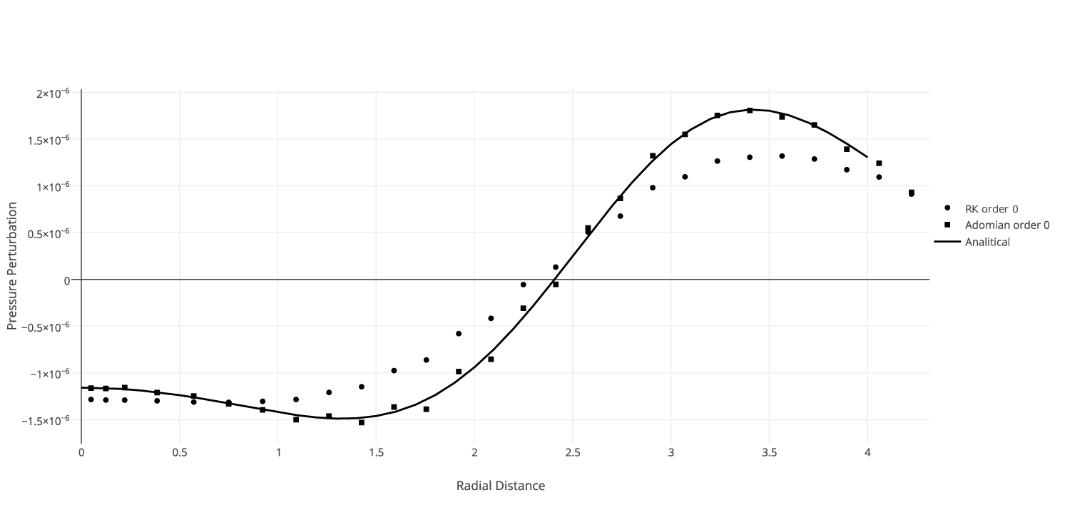
The relative $L^{2}$ error to the exact solution for both RK-DG and ABS-DG schemes are summarized in table 1 for different spatial orders. Results show that ABS-DG yields smaller error values than RK-DG. For instance, ABS-DG first spatial order results are comparable to second-order RK-DG. This is probably explained by the high accuracy of ABS-DG in time, since the employed order is dynamic. In other words, the algorithm computes for each cell the required number of operations such that accuracy satisfies a tolerance at each point of the domain. Figure 2 shows a series of comparison between ABS-DG and RK-DG respect to the exact solution of the propagated Gaussian pulse. We can see that ABS-DG results fit better the exact solution, endorsing results shown in the table.

Table 1: Relative

L^{2}

error for DG vs ABS-DG

Order	DG Method	ABS-DG Method
1	2.75E-001	6.28E-002
2	2.18E-002	2.45E-002
3	2.28E-002	1.26E-003

Cost-effectiveness assessment

Since both RK-DG and ABS-DG have a similar cost per stage, in order to assess the cost-effectiveness of the proposed method, the number of computed stage iterations are compared in table 2 rather than computational time. In the case of ABS-DG, since different number of iterations are performed for each cell, the maximum number of Adomian iterations are counted among all cells. Results indicate that the ABS-DG can reduce the number of iterations by up to 20 times for the first-order and slightly less iterations are needed for the third-order.

The total cost of ABS-DG is therefore smaller than RK-DG for the selected test case. Two arguments in favor of this results are given next. First, it is well accepted now that in order to obtain high accuracy it is better to increase the order of the method rather than refining the grid or time spacing [Kroll2015]. Adomian effectively increases the order in time integration with each additional iteration. Second, ABS-DG seems to be more stable, implying less restrictive CFL conditions (recall previous test case was run with a CFL = 2.5). Despite in this test Adomian requires more stages per time-iteration, the total cost of the method is given by the product of the total number of steps and the number of stages per step.

Finally, the important adaptivity property of the ABS-DG scheme is stressed, which allows for each cell to compute only the required number of iterations to satisfy a tolerance threshold. Hence, big savings are obtained by avoiding irrelevant computations on the fly. This property was not reflected neither in table 2 or in its speedup calculations. As in any adaptive method, reality is case dependent.

Table 2: RK-DG time-iterations VS ABS-DG series terms-iterations for 3 seconds of simulation

Order	DG(Total time iterations)	ABS-DG(Total series terms iterations)
1	300	50
2	300	90
3	300	170

Grid convergence

To study grid convergence of the ABS-DG method, four different meshes with different sizes are generated. This is done by selecting different edge size in SALOME, a tool used to generate meshes on the current work [70]. Simulations are stopped at $t=2$ , and the relative (to the exact) error is computed. Table 3 shows the errors for different $h$ size and in figure 3 their logarithmic curves are plotted. For clarity, each curves is separately shown in figure 4. In dash line the theoretical order of convergence is plotted. The solid line represents the numerical solution. These results demonstrate that we get the right order.

Table 3: Relative error magnitude for several Adomian orders at different Mesh sizes

Order	$h=1.4$	$h=0.7$	$h=0.5$	$h=0.26$
1	5.49E-001	2.80E-001	1.87E-001	8.36E-002
2	2.49E-001	7.69E-002	4.08E-002	1.10E-002
3	7.79E-002	8.36E-003	3.66E-003	3.49E-004

V.II Tests with boundary conditions

The objective of this test is to show how to appropriately impose boundary conditions to the ABS-DG method, since the solution is obtained as a series. Two relevant boundary conditions in aeroacoustic are considered: slip wall and non-reflective conditions. To make the solution fulfill the imposed boundary condition, we force each of the ABS-DG series terms to satisfy them. The slip wall BC are implemented in a weak sense by nullifying the normal to the boundary component of the momentum flux. Non-reflective BC is achieved according to the standard characteristic based non-reflecting boundary conditions. To estimate the accuracy of the ABS-DG and since an exact solution is not available, a $5^{th}$ order RK-DG simulation is run on a fine grid (mesh size of $0.1$ ) and the solution is considered as a reference. The ABS-DG test is run on a mesh with a size of $0.19$ . Simulations are run till $6$ seconds flow time. Table 4 shows the relative (to reference DG solution) error for different ABS-DG orders, we can see that we have a very good agreement with the reference solution and errors are comparable to those obtained in the case of boundary-free tests. Figures 5 and 6 show the propagated pulse obtained by the reference solution and 1st, 2nd and 3rd order (in space) ABS-DG schemes. These tests demonstrate that imposing the boundary conditions on each term of the series for the ABS-DG scheme is an appropriate approach.

Table 4: ABS-DG results compared to reference DG solution (relative error)

Order	Wall condition	Non-reflective condition
1	9.39E-002	9.97E-002
2	3.78E-002	2.27E-002
3	3.50E-003	1.22E-003

VI Conclusions

In this paper a numerical scheme based on the Adomian decomposition method is proposed (ABS). To assess the method, the space derivative operators are discretized using the classical discontinuous Galerkin techniques (ABS-DG). The derivation of the proposed scheme ABS is described in detail, some nice proprieties are proved making the scheme easy to implement and the integration in time very accurate. A connection to the Runge-Kutta time discretization method is established in the linear case, with a clear advantage when using ABS. Indeed, the proven recursive formula makes ABS (or ABS-DG) easy to implement as stated above, being the time-order adaptive and dynamic (no need to set the order in advance) leading to an optimal accuracy with minimum cost. Finally, the ABS-DG scheme performance is assessed by comparison to the classical RK-DG results and the exact solution

Acknowledgments

This research is supported by the Basque Government through the BERC 2014-2017 program and by the Spanish Ministry of Economy and Competitiveness MINECO: BCAM Severo Ochoa accreditation SEV-2013-0323. The authors gratefully acknowledge the financial support of Diputación Foral de Bizkaia (DFB) for this research and the whole BCAM-BALTOGAR project on turbomachinery (grant BFA/DFB-6/12/TK/2012/00020). Imanol Garcia de Beristain was funded by the Basque Government Education Department through the Non Doctoral Researcher Formation Program with reference (PRE_2013_1_1216). Lakhdar Remaki was partially funded by the Project of the Spanish Ministry of Economy and Competitiveness with reference MTM2013-40824-P. Alfaisal University grant IRG with reference IRG16413.

References

[1] Versteeg, H., and Malalasekera, W., 2007. An Introduction to Computational Fluid Dynamics, second edition ed. Pearson Education Limited.
[2] Katate, M., 2013. I do like CFD, VOL.1, Governing Equations and Exact Solutions, second edition ed.
[3] Colonius, T., and Lele, S. K., 2004. “Computational aeroacoustics: progress on nonlinear problems of soundgeneration”. Progress in Aerospace Sciences, 40, pp. 345–416.
[4] Remaki L., Hassan O., M. K., 2011. “Aerodynamic Computations Using a Finite Volume Method with an HLLC Numerical Flux Function”. Mathematical Modelling of Natural Phenomena, 6(3), 1, pp. 189–212.
[5] Olander, M., 2011. “CFD simulation of the volvo cars slotted walls wind tunnel”. Master’s thesis, Department of Applied Mechanics, Chalmers University of Technology,.
[6] Evans, B., Hassan, O., Jones, J., Morgan, K., and Remaki, L., 2011. “Computational fluid dynamics applied to the aerodynamic design of a land-based supersonic vehicle”. Numerical Methods for Partial Differential Equations, 27(1), pp. 141–159.
[7] Remaki, L., Hassan, O., Evans, B., and Morgam, K., 2014. “Spray drag effect of fluidized sand for a supersonic vehicle”. Journal of Coupled Systems and Multiscale Dynamics, 2(3), October, pp. 169–177.
[8] Califano, A., and Steen, S., 2009. “Analysis of different propeller ventilation mechanisms by means of rans simulations”. In First International Symposium on Marine Propulsors, Trondheim, Norway,.
[9] Moshfeghi, M., Song, Y., and Xie, Y., 2012. “Effects of near-wall grid spacing on sst-k-omega model using nrel phase vi horizontal axis wind turbine”. Journal of Wind Engineering and Industrial Aerodynamics,, Volumes 107–108, August–September, pp. 94–105,.
[10] Axerio-Cilies, J., and Iaccarino, G., 2012. “An aerodynamic investigation of an isolated rotating formula 1 wheel assembly”. Journal of Fluids Engineering, 134(12).
[11] Remaki, L., Ramezani, A., Blanco, J. M., and Antolin, J., 2017. “New simplified algorithm for the multiple rotating frame approach in CFD”. Journal of Fluids Engineering, 139(8), pp. 081–104.
[12] Wang1, B., Okamoto, K., Yamaguchi, K. A., and Teramoto, S., 2014. “Loss mechanisms in shear-force pump with multiple corotating disks”. Journal of Fluids Engineering, 136(8).
[13] Yelmule, M., and VSJ, E. A., 2013. “CFD predictions of nrel phase vi rotor experiments in nasa/armes wind tunnel”. International journal of renewable energy research,, 3(2).
[14] Singh, K., Mahajanim, S., Shenoy, K., Patwardhan, A., and Ghosh, S., 2007. “CFD modeling of pilot-scale pump-mixer: Single-phase head and power characteristics”. Chemical Engineering Science, Vol. 22, Issue 5, pp. 1308-1322,.
[15] Lu X and Xie P and Ingham D and Ma L, 2018. “A porous media model for CFD simulations of gas-liquid two-phase flow in rotating packed beds”. Chemical Engineering Science, 189(2), pp. 123–134.
[16] Karthikeyan, T., Abdus, S., and Ezhilsabareesh, K., 2016. “Parametric analysis of a tidal current turbine using CFD techniques”. In Renew 2016 2nd International Conference on Renewable Energies Offshore.
[17] Da-Wen, S., 2019. Computational Fluid Dynamics in Food Processing. CRC Press.
[18] Anandharamakrishnan, C., 2013. Computational Fluid Dynamics Applications in Food Processing. SpringerBriefs in Food, Health, and Nutrition.
[19] Samuelsberg, A., and Hjertager, B. H., 1996. “Computational modeling of gas/particle flow in a riser”. AIChE Journal, 42(6), pp. 1536–1546.
[20] Lutz, A., 2010. Numerical Simulations: Examples and Applications in Computational Fluid Dynamics. InTech.
[21] Ram, K. R., Yogesh, D., and Jitendra, R., 2018. “A review on applications of computational fluid dynamics”. International Journal of LNCT, 2(6), pp. 2456–9895.
[22] Evans, B., Jones, J., Morgan, K., Hassan, O., and Remaki, L., 2010. “Computational fluid dynamics applied to the aerodynamic design of a land-bases supersonic vehicle”. Journal of Partial Differential Equation, 27(1), January, pp. 141–159.
[23] Atmaca, E., Peker, I., and Altin, A., 2005. “Industrial noise and its effects on humans”. Polish Journal of Environmental Studies, 14(6), pp. 721–726.
[24] Christopher, K. W. T., 1995. “Computational aeroacoustics-issues and methods”. AIAA journal, 33(10), pp. 1788–1796.
[25] Colonius, T., and Lele, S. K., 2004. “Computational aeroacoustics: Progress on nonlinear problems of sound generation”. Progress in Aerospace Sciences, 40(6), pp. 345–416.
[26] Lighthill, M. J., 1954. “On sound generated aerodynamically. II. Turbulence as a source of sound”. In Proceedings of the Royal Society of London A: Mathematical, Physical and Engineering Sciences, Vol. 222, The Royal Society, pp. 1–32.
[27] Lighthill, M. J., 1952. “On sound generated aerodynamically. I. General theory”. In Proceedings of the Royal Society of London A: Mathematical, Physical and Engineering Sciences, Vol. 211, The Royal Society, pp. 564–587.
[28] Liever, P. A., West, J. S., and Harris, R. E., 2016. Validation of high-fidelity CFD/CAA framework for launch vehicle acoustic environment simulation against scale model test data. Tech. rep.
[29] Schulze, M., Hummel, T., Klarmann, N., Berger, F., Schuermans, B., and Sattelmayer, T., 2017. “Linearized euler equations for the prediction of linear high-frequency stability in gas turbine combustors”. Journal of Engineering for Gas Turbines and Power, 139(3), pp. 315–325.
[30] Bissuel, A., Allaire, G., Daumas, L., Barre, S., and Rey, F., 2018. “Linearized Navier–Stokes equations for aeroacoustics using stabilized finite elements: Boundary conditions and industrial application to aft-fan noise propagation”. Computers & Fluids, 166, pp. 32–45.
[31] Williamschen, M., Gabard, G., and Bériot, H., 2015. “Performance of the DGM for the linearized Euler equations with non-uniform mean-flow”. In 21st AIAA/CEAS Aeroacoustics Conference, p. 3277.
[32] Xiao-dong, L., Jiang, M., Jun-hui, G., Da-kai, L., Liu, L., and Xiao-yan, L., 2015. “Recent advances of computational aeroacoustics”. Applied Mathematics and Mechanics, 36(1), jan, pp. 131–140.
[33] Kroll, N., Hirsch, C., Bassi, F., Johnston, C., and Hillewaert, K., 2015. IDIHOM-Industrialization of High-Order Methods–A Top Down Approach, Notes on Numerical Fluid Mechanics and Multidisciplinary Design., Vol. 128. Springer International Publishing Switzerland.
[34] Brown, J., 2010. “Efficient nonlinear solvers for nodal high-order finite elements in 3D”. Journal of Scientific Computing, 45(1-3), pp. 48–63.
[35] Huerta, A., Angeloski, A., Roca, X., and Peraire, J., 2013. “Efficiency of high-order elements for continuous and discontinuous Galerkin methods”. International Journal for numerical methods in Engineering, 96(9), pp. 529–560.
[36] DOLEJsi, V., and FELCMAN, J., 2002. “Anisotropic mesh adaptation for transonic and supersonic flow simulation”. In ALGORITMY Conference on Scientific Computing, pp. 78–85.
[37] Peraire, J., Peiró, J., and Morgan, K., 1992. “Adaptive remeshing for three-dimensional compressible flow computations”. Journal of Computational Physics, 103(2), pp. 269 – 285.
[38] Sørensen, K. A., Hassan, O., Morgan, K., and Weatherill, N. P., 2003. “A multigrid accelerated time-accurate inviscid compressible fluid flow solution algorithm employing mesh movement and local remeshing”. International Journal for Numerical Methods in Fluids, 43(5), pp. 517–536.
[39] Habashi, W. G., Dompierre, J., Bourgault, Y., Yahia, A. A., Fortin, M., and Vallet, M. G., 2000. “Anisotropic mesh adaptation: Towards user-independent, mesh-independent and solver-independent CFD solutions: Part I: General principles”. Internat. J. Numer. Methods Fluids, 32, pp. 725–744.
[40] Remaki, L., and Habashi, W., 2006. “3d mesh adaptation on multiple weak discontinuities and boundary layers”. SIAM J. Sci. Comput., 28(4), Jan., pp. 1379–1397.
[41] Zander, N., Bog, T., Kollmannsberger, S., Schillinger, D., and Rank, E., 2015. “Multi-level $hp$ -adaptivity: high-order mesh adaptivity without the difficulties of constraining hanging nodes”. Computational Mechanics, 55(3), pp. 499–517.
[42] da Veiga, L. B., Manzini, G., and Mascotto, L., 2018. “A posteriori error estimation and adaptivity in $hp$ virtual elements”. arXiv preprint arXiv:1804.07898.
[43] Walter, D. J., and Manera, A., 2016. “Adaptive burnup stepsize selection using control theory for 2D lattice depletion simulations”. Progress in Nuclear Energy, 88, pp. 218–230.
[44] Völcker, C., Jørgensen, J. B., Thomsen, P. G., and Stenby, E. H., 2010. “Adaptive stepsize control in implicit Runge-Kutta methods for reservoir simulation”. IFAC Proceedings Volumes, 43(5), pp. 523–528.
[45] Adomian, G., and Rach, R., 1983. “Inversion of nonlinear stochastic operators”. Journal of Mathematical Analysis and Applications, 91(1), pp. 39–46.
[46] Adomian, G., 1994. “Solving frontier problems of physics: The decomposition method”. Kluwer Academic Publishers.
[47] Cherruault, Y., 1998. Modèles et méthodes mathématiques pour les sciences du vivant. Presses Universitaires de France-PUF.
[48] Ebaida, A., Aljoufia, M. D., and Wazwaz, A. M., 2015. “An advanced study on the solution of nanofluid flow problems via Adomian’s method”. Applied Mathematics Letters, 49, pp. 117–122.
[49] Duan, J.-S., Rach, R., Baleanu, D., and Wazwaz, A.-M., 2012. “A review of the Adomian decomposition method and its applications to fractional differential equations”. Communications in Fractional Calculus, 3(2), pp. 73–99.
[50] Wazwaz, A., 2011. Linear and Nonlinear Integral Equations: Methods and Applications. Higher Education Press, Beijing.
[51] Rach, R., Duan, J. S., and Wazwaz, A. M., 2015. “Solving new fourth-order Emden-Fowler type equations by the Adomian decomposition method”. International Journal of Computational Methods in Engineering Science and Mechanics.
[52] Singh, R., and Wazwaz, A., 2015. “An efficient semi-numerical technique for solving nonlinear singular boundary value problems arising in various physicsal models”. nternational J. Of Computer Mathematics.
[53] Momani, S., and Odibat, Z., 2006. “Analytical solution of a time-fractional Navier-Stokes equation by Adomian decomposition method”. Applied Mathematics and Computation, 177, pp. 488–494.
[54] Khan, N., Ara, A., Anwer Ali, S., and Mahmood, A., 2009. “Analytical study of Navier–Stokes equation with fractional orders using He’s homotopy perturbation and variational iteration methods”. International Journal of Nonlinear Sciences and Numerical Simulation, 10, 02, pp. 1127–1134.
[55] Vahidi, A., and Jalalvand, B., 2012. “Improving the accuracy of the adomian decomposition method for solving nonlinear equations”. Applied Mathematical Sciences, 6(10), pp. 487 – 497.
[56] Gbadamosi, B., Adebimpe, O., Akinola, E. I., and A., O. I., 2012. “Solving Riccati equation using Adomian decomposition method”. International Journal of Pure and Applied Mathematics, 78(3), pp. 409–417.
[57] Alabdullatif, M., Abdusalam, H. A., and Fahmy, E. S., 2007. “Adomian decomposition method for nonlinear reaction diffusion system of Lotka-Volterra type”. In International Mathematical Forum, Vol. 2, pp. 87–96.
[58] Mohyud-din, S. T., Noor, M. A., and Noor, K. I., 2010. “Variational iteration method for Burgers’ and coupled Burgers’ equations using He’s polynomials”. pp. 263–267.
[59] Zhu, H., Shu, H., and Ding, M., 2010. “Numerical solutions of two-dimensional Burgers’ equations by discrete Adomian decomposition method”. Computers & Mathematics with Applications, 60(3), pp. 840–848.
[60] Chen, Y., and An, H. L., 2008. “Numerical solutions of coupled Burgers equations with time- and space-fractional derivatives”. Applied Mathematics and Computation, 200, pp. 87–95.
[61] Birajdar, G. A., 2014. “Numerical solution of time fractional Navier–Stokes equation by discrete Adomian decomposition method”. Nonlinear Engineering, 3(1), pp. 21–26.
[62] Rydin, Y., 2016. “Modeling sound propagation from wind turbines using linearized 3d euler equations”. PhD thesis, Uppsala University, Division of Scientific Computing.
[63] Imanol, G. d. B., 2018. “On adomian based numerical schemes for euler and navier-stokes equations and application to aeroacoustics propagation”. PhD thesis, UPV, University Spain.
[64] Blom, C. P. A., 2003. “Discontinuous galerkin method on tetrahedral elements for aeroacoustics”. PhD thesis, Ph.D. thesis, University of Twente, Enschede, The Netherlands.
[65] Shu, C.-W., and Atkins, H. L., 1998. “Quadrature-free implementation of discontinuous Galerkin method for hyperbolic equations”. AIAA Journal, 36(5), May, pp. 775–782.
[66] Cockburn, B., Karniadakis, G. E., and Shu, C.-W., 1999. “The development of discontinuous Galerkin methods”. IMA Preprint Series No. 1662.
[67] Lummer, M., 2016. “A hybrid 3d discontinuous galerkin code for caa applications”. In 22nd AIAA/CEAS Aeroacoustics Conference, p. 2719.
[68] Masatsuka, K., 2013. I do like CFD, VOL.1, Second Edition. No. v. 1. K. Masatsuka.
[69] Tam, C., and Webb, J., 1993. “Dispersion-relation-preserving finite difference schemes for computational acoustics”. Journal of Computational Physics, 107(2), p. 262–281.
[70] Bergeaud, V., and Lefebvre, V., 2010. “Salome. a software integration platform for multi-physics, pre-processing and visualisation”.
[71] Chalmers, N., 2015. “c”. PhD thesis, University of Waterloo.
[72] Emery, A. F., 1968. “An evaluation of several differencing methods for inviscid fluid flow problems”. Journal of Computational Physics, 2(3), pp. 306 – 331.
[73] Woodward, P., and Colella, P., 1984. “The numerical simulation of two-dimensional fluid flow with strong shocks”. Journal of computational physics, 54(1), pp. 115–173.
[74] Chu, B.-T., and Kovásznay, L. S. G., 1958. Non-linear interactions in a viscous heat-conducting compressible gas.