Differentiable Robotic Manipulation of Deformable Rope-like Objects Using Compliant Position-based Dynamics
Abstract
Robot manipulation of rope-like objects is an interesting problem that has some critical applications, such as autonomous robotic suturing. Solving for and controlling rope is difficult due to the complexity of rope physics and the challenge of building fast and accurate models of deformable materials. While more data-driven approaches have become more popular for finding controllers that learn to do a single task, there is still a strong motivation for a model-based method that could be used to solve a large variety of optimization problems. Towards this end, we introduced compliant, position-based dynamics (XPBD) to model rope-like objects. Using geometric constraints, the model can represent the coupling of shear/stretch and bend/twist effects. Of crucial importance is that our formulation is differentiable, which can solve parameter estimation problems and improve the matching of rope physics to real-life scenarios (i.e., the real-to-sim problem). For the generality of rope-like objects, two different solvers are proposed to handle the inextensible and extensible effects of varied material stiffness for the rope. We demonstrate our framework’s robustness and accuracy on real-to-sim experimental setups using the Baxter robot and the da Vinci research kit (DVRK) [1]. Our work leads to a new path for robotic manipulation of the deformable rope-like object taking advantage of the ready-to-use gradients.
I Introduction
For problems in grasping soft objects, modeling and simulation of deformable objects have recently been considerable interest in many robotic applications [2, 3], to manipulating soft tissue [4, 5], cloth [6, 7], and even fluids [8, 9]. Among soft structures, deformable linear objects (DLOs), including rope-like objects, strings, cables, beams, etc., are studied (cable routing [10], wire insertion [11], flexible rope [12], and knotting of surgical thread [13]). Recently, techniques involving visual servoing [14, 15], latent dynamics learning [16], and adaptive estimation [17], have all be explored for controlling DLOs. Further reviews in this space can be found in review papers on the topic [18, 19, 20].
Classical methods for modeling rope reside from Cosserat rod theory [21] which involves an analytical, partial differential equation representing the rope as a continuous 3D-dimensional curve exhibiting both bending and torsion. However, the analytical dynamics are limited by the computational efficiency and stability of solving this PDE with two-point boundary conditions (given by the start and end of the rope).
Alternative to exact analytical models, a model-free method may try to identify representations of rope using purely visual descriptors from a camera without involving classical mechanics. These model-free representations include curvature and Fourier-based shapes [22, 23], as well as neural network features [24, 25, 26]. Instead of directly modeling physical mechanics, the state space representation is embedded in these latent space features. However, these approaches need a large quantity and variety of data for training, which is not easy to get in field robotic applications (either in simulation or real life). Meanwhile, the collected datasets are limited to the distribution of objects manipulated. Thus models that learn from simulation or limited real-world data encounter a real-to-sim transfer challenge or an over-fitting problem, respectively.

An increasing number of simulators are made available for robot learning involving rope-like objects [27, 28]. These simulators have been focused on their use for data generation and lack a method for integration in a model-based control context.In general, many existing robotics simulators (including the above, as well as Bullet [29]) and Gym [30], unable to simulate soft bodies) only support gradient calculations based on finite differences. However, differentiable physics and simulation have become critical features for the robot learning community [31]. The works in [32, 33, 34, 35] have applied differentiable framework into rigid articulated body simulation, while others have done the same for deformable objects [36, 37, 38]. These methods provide gradients within the differentiable framework, where optimization tasks for modeling and control are natively supported. Meanwhile, the differentiability can be easily deployed into neural layers for learning-based methods, such as in [39, 40].
One simulation approach that has gained significant interest due to its speed, stability, and capability to model the spectrum from rigid to soft to liquid is Position-based dynamics (PBD) [41, 42]. Unlike the traditional Lagrangian force-based method, the geometric position constraints are solved iteratively. Simulating soft objects involves utilizing the Compliant Position-based Dynamics (XPBD) method [43] which has been shown for a variety of deformable solid bodies, cloth, and chains. Some researchers have directly integrated the Cosserat model into PBD simulators to define the twist and bend, stretch and shear the a the constraints, by introducing particles with orientation information to describe angular updates [44]. Next, the authors added scale parameters for rope-like objects to preserve volume consistency [45]. Although several works have been applied for real-to-sim tasks of soft deformable tissue [4, 5], rigid articulated robots [46], and fluids [8, 47], with constraint-based formulation of PBD or XPBD. However, there is a missing combination of modeling and control approaches applied to rope-like objects in literature, exploiting the capability of XPBD.
In the paper, we propose a solution to formulate a real-to-sim modeling and control framework. We extended the original position-based dynamics (PBD) for rope-like objects proposed in [44] with a compliance parameter by following the XPBD work in [43]. Meanwhile, it is deployed differently using the automatic differentiation functionality available in PyTorch for gradient updates. The new compliant position-based dynamics (XPBD) for rope-like objects can guarantee stable forward simulation while the back-propagation of losses can be applied for modeling and control tasks and parameter identification. The contributions of this paper are as follows:
- •
We describe rope-like objects as a compliant position-based dynamics (XPBD) model by constructing geometrical constraints defining their behaviors.
- •
We introduced a differentiable framework for modeling and simulation that works well with auto-differentiation and algorithm configurations for constraint solving.
- •
We defined the problem of parameter identification and manipulation control of rope-like objects in real-to-sim context (Fig. 1).
- •
We validate our methods in real-world experiments using robot manipulators (Baxter) and surgical robots (dVRK).
II Methods
II-A Compliant Position-Based Dynamics (XPBD) Modeling of Rope-like Object
The XPBD method will be a foundation for building the differentiable model for DLOs. We firstly discretize the DLO into a sequence of particles (Fig. 2) with Cartesian coordinates . Meanwhile, quaternions are used to describe orientations in-between adjacent particles , and will be used to solve the bending and twist deformation of the DLO. Unlike force-based methods such as Euler-Bernoulli beam or Cosserat rod theory, full strain and torsion deformations can be updated with a position-based dynamics solver. As with all simulations using PBDs, the methods starts with a list of constraints, that describe the dynamics of particles. Solving the constraints involves updating and directly using a non-linear projected Jacobi method used for constrained optimization problems. The method to solve for the gradient updates is derived below.
Constraints can be linearized by Taylor series expansion,
| (1) |
with
| (2) |
where the Lagrange multiplier change can be found by introducing the compliance parameter [43],
| (3) |
where and are the weighted terms to guarantee the conservation of linear and angular momentum. Generally, it refers to the mass/inertia matrix as and . For simplification of DLOs, we use uniformed scalar weights instead of matrices for each dimensionality, which has not much impact on simulation and dynamical performance but reduces computational load. That is,
| (4) |
Next, we will introduce several geometrical constraints to simulate the behaviors of the DLOs.
II-A1 Shear and Stretch Constraint
According to Cosserat theory, the shear and stretch measures the deformation regarding the tangent direction of the rope-like object. Therefore, the stretch/compressed length should be constrained relative its rest pose, which indicates in-extensible elasticity. Simultaneously, the normal direction (i.e., the rotated from world frame noted by ) for each cross-section should be parallel to the tangent direction of object’s centerline, see Fig. 2. It measures the shear strain with respect to non-deformed states. Thus, for each pair of neighboring particles, the shear-stretch deformation can be integrated into a generalized constraint as, , which is,
| (5) |
where is the rotation matrix from the local frame of line segment to world frame represented using quaternion, represent the states in rest pose. According to gradient calculation in [44], we can obtain,
| (6) |
Where is the skew-symmetrical matrix representation of a vector.
II-A2 Bend and Twist Constraint
In differential geometry, the Darboux vector is used to parameterize strain deformation with respect to frame rotation. According to Cosserat theory, the Darboux vector can be expressed as a quaternion by measuring the rod’s twist in the tangent direction. Thus, the difference between the current and resting configuration should be evaluated, i.e. . According to [44], the bend and twist constraint can be computed for each pair of two adjacent quaternions (shown in Fig. 2) by, , which is,
| (7) |
where is the imaginary part of the quaternion and is the conjugate quaternion. The constraint gradients can be calculated as,
| (8) |
II-A3 Distance Constraint
One property of modeling ropes is that they can be considered either extensible or inextensible based on how stiff they are, and ultimately this can be modeled as a constraint. Although the above strain deformation have considered the inextensible property implicitly, the iterative solver in Eq. 2 cannot guarantee that all the constraints will be satisfied. Therefore, we can explicitly consider the distance constraint for an enhanced inextensible chain structure using only discretized particle positions. We define by,
| (9) |
The gradients can be easily obtained by,
| (10) |
II-B Real-to-Sim Parameter Identification
Given the above constraints, the dynamics of a rope-like object can be represented by a set of discretized particles (shown in Fig. 2) with position and orientation evolution. However, it is just an approximation of the real model for the rope objects.
For the above shear/shear, bend/twist and distance constraints, we can introduce the additional stiffness parameter to weight the updates during iteration steps, namely by,
| (11) |
Which stands for shear/stretch, bend/twist, and distance constraints regarding position or orientation. Moreover, stands for position changes due to external gravity, and stands for the successive over-relaxation parameter and is applied to accelerate the convergence speed further. Thus, we can introduce the above parameters in a real-to-sim setup by inserting them into the following differentiable framework.
II-C Differential Framework
To perform an optimal control task, the ready-to-use gradients will be needed to compute. We introduce the compliant position-based dynamics (XPBD) inside a differentiable framework, as shown in Algorithm 1 11 1 In this paper, we only consider the quasi-static dynamical states. Only the gravity will be regarded as without any external torques. Thus, the Euler prediction and integration of velocity and angular speed will not be involved.. We rely on the automatic differentiation function provided by PyTorch to obtain the gradients. It can be natively integrated into optimization or learning methods, since the coding framework can be viewed as a differentiable layer which support both forward and backpropagation operations. The computing memory might be limited by the number of iterations for substep simulation. Denoting the gradient variable at time by , we can formulate the following optimization problem as,
| (12) |
where , and are the position-based constraints, and is the loss function derived from the system states. represents the selected gradient variable, which can be control states, system parameters or system states.
2
3
5
6
7
8
9
10
III Real-to-Sim and Shape Control Problem Setup
In this part, we used the proposed differentiable framework to conduct three different experiments both on Rethink Baxter and the da Vinci Research Kit (dVRK) robotic platforms. The Baxter represents a situation of more significant rope manipulation, whereas the dVRK represents a situation of surgical automation involving blood vessel manipulation. We considered the Baxter-rope experiment to involve an inextensible DLO, while the dVRK blood-vessel experiment to be an extensible DLO. For both setups, we looked at both a real-to-sim problem (i.e., parameter estimation based on observations from the real world), and a control problem (i.e., using the XPBD model we developed to have rope configuration reach a target configuration iteratively). The implementation of each experiment will be provided later.
III-A Solver Setups
In classical PBD solver [41], the Jacobi approach averages each constraint step changes, and keeps updating iteratively. The convergence compromises between the number of iterations and the satisfaction of other constraints. However, it was not suitable for simulation of the inextensible effects for ropes with significant axial stiffness.
Precisely, we needed to guarantee the fulfillment of the distance constraint in Eq. 9 completely. A direct linear solver was proposed [48] based on the tridiagonal matrix algorithm, i.e., Thomas algorithm, to preserve the inextensible characteristics of rope-like objects. We will refer to methods individually as the Jacobi XPBD and Thomas XPBD, respectively. All other constraints, such as shear/stretch and bend/twist constraints, used the Jacobi method.22 2 Thus, in this paper, when Jacobi XPBD and Thomas XPBD are indicated, it is distinguishing how the distance constraint is solved.
III-B Data Preprocessing
In our experiments, we obtained both the point cloud and RGB image data using the Microsoft Azure Kinect. For the 2D images obtained, we extracted the centerline of the rope using MATLAB skeletonization function33 3 https://www.mathworks.com/help/images/ref/bwskel.html. Since the raw point cloud data was noisy, we projected them to a hyperplane defined by the gravity vector and two endpoints of the rope, as shown in Fig. 3. The projected point cloud was constrained within a plane, which was easier for identification of bend/twist effects. We used the de-noised 2D centerline from the image and projected 3D point clouds as ground truth data for loss computation in the following section.
 |
 |
III-C Loss Functions
We defined four types of primary losses to investigate for shape matching. We looked at the combinations of these losses for ablation, resulting in 9 different aggregate loss functions for optimization. The loss functions are shown in Table I.
- •
Point-to-Line : As shown in Fig. 4, we intended to find the minimum distance from each preprocessed real data point , to the line segments between each pair of adjacent simulated particle . Thus, the primary loss regarding point-to-line loss was
(13) where we discretized the rope to particle nodes, along preprocessed real data points, and was the projected locations on each line segment with minimum distance.
- •
Segment-to-Particle : We splitted the real data points (preprocessed for noises and re-ordered) into different segments along the vector formulated by two rope endpoints, i.e. , etc shown in Fig. 4. The start/endpoints (i.e., , ) of each segment were determined according to the proportional length to the whole data set. We evaluated the distance between the start/endpoints of each segment and the corresponding particle in the simulation. Then, the segment-to-particle loss was,
(14) - •
Segment-to-Line : As above, we already divided the real data into segments. The projection distance between all points in each segment set () and the corresponding line segment () could be used to evaluate the loss. Thus, the segment-to-line loss was,
(15) where was the number of real data points for each segment group set, and was the projected locations on the line segment with minimum distance.
- •
Lowest 3D Point Along Gravity Vector : The lowest point along the gravity direction of the denoised real data was compared with the one in simulation. This could compensate for lacking depth information while using the 2D centerline. The loss was defined as,
(16)
In our experiments, the point-to-line, segment-to-particle, and segment-to-line losses could be applied to either the 3D point cloud or 2D centerline. We performed 9 different combinations of types of losses as shown in Table I. The loss function , , contained 3D information only, while , , were considering 2D cases only. , , were applied to both 2D cases and the included 3D lowest point with depth information.
| Symbol | |||||||||
| Loss | |||||||||
| Meaning | Point-to-Line for 3D and 2D | Segment-to-Particle for 3D and 2D | Segment-to-Line for 3D and 2D | ||||||
IV Experiments And Result Analysis
IV-A Inextensible Rope Parameter Identification
Parameter identification and position estimation of the control point were carried out on an inextensible rope manipulated by the Baxter robot. We fixed one endpoint of the rope to the environment, and the other endpoint of the rope to the manipulator end-effector (referred as the control point). We continuously moved the control point and collected 36 frames of point cloud for the rope deformation. The Microsoft Azure Kinect was used to obtain the 2D RGB image frames for centerline extraction at the same time. Since only translational movement (fixed rotation angle) of end-effector is controlled, the point cloud had occlusions and was not fully visible at the local region near the control point. We applied the keypoint-based kinematics reconstruction from [49] to identify the 3D position of the control point. Therefore, the ground truth data for 3D point cloud and 2D centerline, as well as control point were ready for real-to-sim transfer.
In XPBD simulation, considering the computational cost and stiffness of the rope, the number of particle were set by . was the control point and corresponding to the endpoint was fixed to the environment. According to Section II-B, there were six constraint stiffness parameters needed to estimate, as shown in Table II. Because 3D point cloud could be more informative than 2D centerline which lacked depth data, the parameters were optimized with using the 3D point-to-line loss. We then estimated the position of the control point (i.e. , see Algorithm 1) using all loss functions in Tab. I to evaluate the accuracy of parameter identification.
For parameter identification, a single gravity parameter was inferred based on Thomas solver, the comparison of simulated results before and after parameter optimization was shown in Fig. 5. After parameter optimization, the simulation states was approximately approaching to the ground truth point cloud. As for the Jacobi solver, it needed two sets of gravity stiffness to deal with different convergency of distance constraint for varied rope states (bending and tensioned), as shown in Table. III.
| Parameter | Initial | Optimized | Meaning |
| 0.04 | 0.024 | position stiffness (gravity) | |
| 1.0 | 0.48 | position stiffness (distance) | |
| 1.0 | 1.16 | position stiffness (shear/stretch) | |
| 1.0 | 0.52 | quaternion stiffness (shear/stretch) | |
| 1.0 | 1.49 | quaternion stiffness (bending/twist) | |
| 1.0 | 0.61 | successive over-relaxation weight |
 |
 |
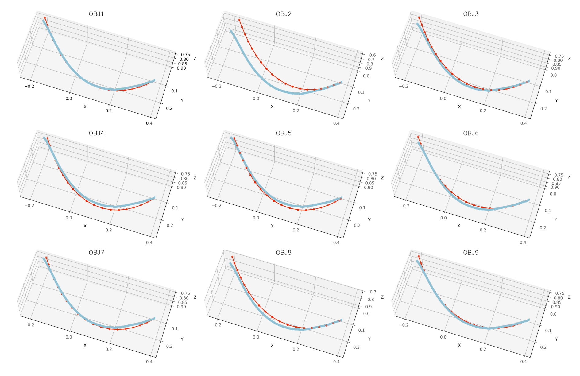
For position estimation of control point, we made a comparison over the nine kinds of loss functions shown in Table I firstly. The 3D point cloud included the rope information in 3D space, while the 2D centerline did not contain depth information. As a result, the simulation result containing the 3D information showed the best performance, i.e., , , and as shown in the Fig. 7. For , , and , whose loss function consisted of 2D information and partial 3D information (the lowest point along gravity direction), the simulation result was improved compared to , , and , which only considered 2D information. As shown in Fig. 7 and Fig. 6 , obtained the best performance among all these losses. It simply proved the accuracy of parameter identification, and showed that the 3D data contributed more than 2D cases for control point estimation.



 |
 |
We also compared the performance of Thomas XPBD and Jacobi XPBD when estimating the position of the control point. The middle plot in Fig. 13 showed the rope length change of the simulated result from 36 frames. The average length deviation over the ground truth length for Thomas XPBD solver was for all structures, but for Jacobi solver, it was . Especially when the rope became tense, the error for Jacobi solver became more significant. The same phenomenon occurred on the error of the control point’s position in Fig. 9. The left and right plots in Fig. 13 indicated that the distance constraint in the Jacobi XPBD was hard to be satisfied when the rope was approaching the tensioned status. The Jacobi XPBD intuitively tried to comprise the satisfaction of each constraint solving. It iteratively struggled to maintain the stretch, twist, and distance against gravity. Thus, it resulted in a no-complete convergency of distance constraint . For Thomas XPBD, the distance constraint would be satisfied between each neighboring node simultaneously within one step solving, which was similar as the position update mechanism of the gravity. In this case, Thomas XPBD solver ensured that the length of rope was unchanged, and it was more suitable for the simulation of inextensible rope. The simulation result shown in Fig. 8 proved our conclusion.
IV-B Extensible Rope Parameter Identification and Key Points Estimation
Parameter identification and position estimation of control point were carried out on an extensible, flexible silicone rod using the dVRK surgical robot. The silcone rod was chosen to resemble a compliant and dissected vessel, a technique that is often used in surgery to avoid damaging the vessel. The two endpoints of the rope were fixed, and the control point was in the middle of the rope. We moved the control point to collect 30 frames of point cloud data. In simulation, the number of particle nodes were . and corresponding to both the endpoints were fixed and was the control point. We did not need to preserve the inextensible behavior completely since the silicon rope had a lower axial stiffness. Thus, we only implemented the Jacobi XPBD solver for the distance constraint in this experiment. The loss function used was in Table I, and we estimated the same parameters as the ones indicated in Section II-B. After parameter estimation, we estimated the position of the control point (i.e. ) using and , i.e., point-to-line for both 3D and 2D cases. For parameter identification, we used grid-search to identify the optimized six parameters in Table III for extensible rope. Since the control point was set at the middle of the rope, manipulation could result in one side being tight and the other being loose. Thus, the effect of the gravity over two sides was different, and we needed to define different gravity weights for the two sides, as shown in Fig. 10.
| Parameter | Inextensible rope | extensible rope |
| 0.26 (bending) / 0.001 (tensioned) | 25 (relax) / 3 (tensioned) | |
| 1.19 | 0.87 | |
| 0.80 | 0.873 | |
| 1.19 | 1.0 | |
| 0.80 | 1.30 | |
| 0.79 | 0.61 |
 |
 |
 |
With the optimized parameters, we estimated the position of the control point and a reference point, namely by key points. Apart from the control point, there was a reference point with a red marker, shown in Fig. 10. The marker was used only for comparison between ground truth trajectory and simulation result in Fig. 12 Right and not for parameter estimation. Fig. 12 Left showed the error curve of the location of reference and control point. Even though the raw data of the extensible rope was noisier, the average error of the control point and the reference point was acceptable, which proved the robustness of our solver. In Fig. 11, we showed the original image and simulation result for different frames, and no matter how the rope deformed, our solver could get a desirable outcome. Even though Thomas solver outperformed the Jacobi solver in the previous experiment, Thomas XPBD was too tough to simulate the silicon rope. Thomas XPBD required the length of the rope to remain unchanged, which contradicted the silicon rope’s extensible property. Thus, the Thomas solver diverged for the simulation, and the Jacobi solver was more suitable.

IV-C Inextensible Rope Shape Control
Based on the Thomas XPBD solver, the shape control task was carried out on the same Baxter setup as the Section IV-A. The ground truth shape of the rope was obtained by locating the left control point (end-effector), right fixed endpoint and the middle three Aruco Markers shown [50] in the Fig. 1 and Fig. 14. We fixed the simulated rope to the same right endpoint. By setting the middle three points as the shape target, we optimized the position of the control point from the differentiable Thomas XPBD simulation.
As shown in Fig. 14, the transparent rope with low opacity was our shape control target status, and the solid ones with high opacity were the result controlled by the identified parameters from Section IV-A. Our controlled shape could almost overlap with the target rope, as shown in the Top Row of Fig. 14. However, some had deviations as shown in the Bottom Row of Fig. 14. One of the reason is we only considered three shape points as the target for loss computation. The accuracy will be improved by considering more discretized segments of the ground truth data. Another reason was because we did not consider the rotational control of the end-effector when solving the inverse kinematics of the Baxter, which caused the rope not to be able to move to the desired position perfectly.
V Conclusion and Future Works
This paper used a compliant position-based framework to conduct the differential real-to-sim tasks for parameter identification and shape control tasks. Several geometrical constraints were introduced to model the rope-like objects’ coupling stretch/shear and bending/twisting effects. To inspect the inextensible and extensible impact, the Thomas solver and the Jacobi solver are proposed for the distance constraint. The experiment results on the Baxter robot and DVRK platform proved the validity and robustness of our solvers. The shape control tasks showed a novel path for real-to-sim robotic manipulation operations.
The future works will consider differentiable control with collision handling and rigid-deformable coupling. Meanwhile, more advanced tasks will be considered, such as surgical thread manipulation in field environments using the proposed inextensible solver.
Acknowledgement
Many thanks to Yutong Zhang for the rendering of the cover photo. This work was supported by NSF CAREER award 2045803 and the US Army Telemedicine and Advanced Technologies Research Center.
References
- [1] C. D’Ettorre, A. Mariani, A. Stilli, F. Rodriguez y Baena, P. Valdastri, A. Deguet, P. Kazanzides, R. H. Taylor, G. S. Fischer, S. P. DiMaio, et al., “Accelerating surgical robotics research: A review of 10 years with the da vinci research kit,” IEEE Robotics and Automation Magazine, 2021.
- [2] I. Huang, Y. Narang, C. Eppner, B. Sundaralingam, M. Macklin, T. Hermans, and D. Fox, “Defgraspsim: Simulation-based grasping of 3d deformable objects,” 2021.
- [3] Y. Han, R. Batra, N. Boyd, T. Zhao, Y. She, S. Hutchinson, and Y. Zhao, “Learning generalizable vision-tactile robotic grasping strategy for deformable objects via transformer,” CoRR, vol. abs/2112.06374, 2021. [Online]. Available: https://arxiv.org/abs/2112.06374
- [4] F. Liu, Z. Li, Y. Han, J. Lu, F. Richter, and M. C. Yip, “Real-to-sim registration of deformable soft tissue with position-based dynamics for surgical robot autonomy,” in 2021 IEEE International Conference on Robotics and Automation (ICRA), 2021, pp. 12 328–12 334.
- [5] Y. Han, F. Liu, and M. C. Yip, “A 2d surgical simulation framework for tool-tissue interaction,” 2021.
- [6] R. Hoque, D. Seita, A. Balakrishna, A. Ganapathi, A. Tanwani, N. Jamali, K. Yamane, S. Iba, and K. Goldberg, “VisuoSpatial Foresight for Multi-Step, Multi-Task Fabric Manipulation,” in Robotics: Science and Systems Current file Overview 8 (RSS), 2020.
- [7] Y. Wu, W. Yan, T. Kurutach, L. Pinto, and P. Abbeel, “Learning to Manipulate Deformable Objects without Demonstrations,” in Proceedings of Robotics: Science and Systems, Corvalis, Oregon, USA, July 2020.
- [8] J. Huang, F. Liu, F. Richter, and M. C. Yip, “Model-predictive control of blood suction for surgical hemostasis using differentiable fluid simulations,” in 2021 IEEE International Conference on Robotics and Automation (ICRA), 2021, pp. 12 380–12 386.
- [9] C. Schenck and D. Fox, “Spnets: Differentiable fluid dynamics for deep neural networks,” in Proceedings of the Second Conference on Robot Learning (CoRL), Zurich, Switzerland, 2018.
- [10] D. McConachie, T. Power, P. Mitrano, and D. Berenson, “Learning when to trust a dynamics model for planning in reduced state spaces,” IEEE Robotics and Automation Letters, vol. 5, no. 2, pp. 3540–3547, 2020.
- [11] R. Lagneau, A. Krupa, and M. Marchal, “Automatic shape control of deformable wires based on model-free visual servoing,” IEEE Robotics and Automation Letters, vol. 5, no. 4, pp. 5252–5259, 2020.
- [12] F. Zhong, Y. Wang, Z. Wang, and Y.-H. Liu, “Dual-arm robotic needle insertion with active tissue deformation for autonomous suturing,” IEEE Robotics and Automation Letters, vol. 4, no. 3, pp. 2669–2676, 2019.
- [13] B. Lu, W. Chen, Y. Jin, D. Zhang, Q. Dou, H. K. H. Chu, P. Heng, and Y. Liu, “A learning-driven framework with spatial optimization for surgical suture thread reconstruction and autonomous grasping under multiple topologies and environmental noises,” CoRR, vol. abs/2007.00920, 2020. [Online]. Available: https://arxiv.org/abs/2007.00920
- [14] J. Zhu, “Vision-based robotic manipulation of deformable linear objects,” Theses, Université Montpellier, Mar. 2020. [Online]. Available: https://tel.archives-ouvertes.fr/tel-02971484
- [15] J. Zhu, D. Navarro-Alarcon, R. Passama, and A. Cherubini, “Vision-based Manipulation of Deformable and Rigid Objects Using Subspace Projections of 2D Contours,” Robotics and Autonomous Systems, May 2021. [Online]. Available: https://hal.archives-ouvertes.fr/hal-02558064
- [16] W. Zhang, K. Schmeckpeper, P. Chaudhari, and K. Daniilidis, “Deformable linear object prediction using locally linear latent dynamics,” in 2021 IEEE International Conference on Robotics and Automation (ICRA). IEEE, may 2021. [Online]. Available: https://doi.org/10.1109%2Ficra48506.2021.9560955
- [17] M. Yu, H. Zhong, and X. Li, “Shape control of deformable linear objects with offline and online learning of local linear deformation models,” 2021.
- [18] H. Yin, A. Varava, and D. Kragic, “Modeling, learning, perception, and control methods for deformable object manipulation,” Science Robotics, vol. 6, no. 54, p. eabd8803, 2021. [Online]. Available: https://www.science.org/doi/abs/10.1126/scirobotics.abd8803
- [19] J. Sanchez, J.-A. Corrales, B.-C. Bouzgarrou, and Y. Mezouar, “Robotic manipulation and sensing of deformable objects in domestic and industrial applications: a survey,” The International Journal of Robotics Research, vol. 37, no. 7, pp. 688–716, 2018.
- [20] J. Zhu, A. Cherubini, C. Dune, D. Navarro-Alarcon, F. Alambeigi, D. Berenson, F. Ficuciello, K. Harada, J. Kober, X. Li, J. Pan, W. Yuan, and M. Gienger, “Challenges and Outlook in Robotic Manipulation of Deformable Objects,” IEEE Robotics and Automation Magazine, 2021. [Online]. Available: https://hal.archives-ouvertes.fr/hal-03483491
- [21] M. Gazzola, L. Dudte, A. McCormick, and L. Mahadevan, “Forward and inverse problems in the mechanics of soft filaments,” Royal Society open science, vol. 5, no. 6, p. 171628, 2018. [Online]. Available: https://doi.org/10.1098/rsos.171628
- [22] D. Navarro-Alarcon, Y. hui Liu, J. G. Romero, and P. Li, “On the visual deformation servoing of compliant objects: Uncalibrated control methods and experiments,” The International Journal of Robotics Research, vol. 33, no. 11, pp. 1462–1480, 2014. [Online]. Available: https://doi.org/10.1177/0278364914529355
- [23] D. Navarro-Alarcon and Y.-H. Liu, “Fourier-based shape servoing: A new feedback method to actively deform soft objects into desired 2-d image contours,” IEEE Transactions on Robotics, vol. 34, no. 1, pp. 272–279, 2018.
- [24] P. Sundaresan, J. Grannen, B. Thananjeyan, A. Balakrishna, J. Ichnowski, E. Novoseller, M. Hwang, M. Laskey, J. Gonzalez, and K. Goldberg, “Untangling Dense Non-Planar Knots by Learning Manipulation Features and Recovery Policies,” in Proceedings of Robotics: Science and Systems, Virtual, July 2021.
- [25] S. Huo, A. Duan, C. Li, P. Zhou, W. Ma, and D. Navarro-Alarcon, “Keypoint-based bimanual shaping of deformable linear objects under environmental constraints using hierarchical action planning,” CoRR, vol. abs/2110.08962, 2021. [Online]. Available: https://arxiv.org/abs/2110.08962
- [26] A. Wang, T. Kurutach, K. Liu, P. Abbeel, and A. Tamar, “Learning robotic manipulation through visual planning and acting,” in Proceedings of Robotics: Science and Systems, FreiburgimBreisgau, Germany, June 2019.
- [27] R. Laezza, R. Gieselmann, F. T. Pokorny, and Y. Karayiannidis, “Reform: A robot learning sandbox for deformable linear object manipulation,” in 2021 IEEE International Conference on Robotics and Automation (ICRA), 2021, pp. 4717–4723.
- [28] X. Lin, Y. Wang, J. Olkin, and D. Held, “Softgym: Benchmarking deep reinforcement learning for deformable object manipulation,” in Conference on Robot Learning, 2020.
- [29] E. Coumans and Y. Bai, “Pybullet, a python module for physics simulation for games, robotics and machine learning,” http://pybullet.org, 2016–2021.
- [30] G. Brockman, V. Cheung, L. Pettersson, J. Schneider, J. Schulman, J. Tang, and W. Zaremba, “Openai gym,” arXiv preprint arXiv:1606.01540, 2016.
- [31] Y. Hu, L. Anderson, T.-M. Li, Q. Sun, N. Carr, J. Ragan-Kelley, and F. Durand, “Difftaichi: Differentiable programming for physical simulation,” 2020.
- [32] F. de Avila Belbute-Peres, K. Smith, K. Allen, J. Tenenbaum, and J. Z. Kolter, “End-to-end differentiable physics for learning and control,” in Advances in Neural Information Processing Systems, S. Bengio, H. Wallach, H. Larochelle, K. Grauman, N. Cesa-Bianchi, and R. Garnett, Eds., vol. 31. Curran Associates, Inc., 2018. [Online]. Available: https://proceedings.neurips.cc/paper/2018/file/842424a1d0595b76ec4fa03c46e8d755-Paper.pdf
- [33] Y.-L. Qiao, J. Liang, V. Koltun, and M. C. Lin, “Efficient differentiable simulation of articulated bodies,” in Proceedings of the 38th International Conference on Machine Learning, ser. Proceedings of Machine Learning Research, M. Meila and T. Zhang, Eds., vol. 139. PMLR, 18–24 Jul 2021, pp. 8661–8671.
- [34] K. Werling, D. Omens, J. Lee, I. Exarchos, and C. K. Liu, “Fast and Feature-Complete Differentiable Physics Engine for Articulated Rigid Bodies with Contact Constraints,” in Proceedings of Robotics: Science and Systems, Virtual, July 2021.
- [35] F. Liu, M. Li, J. Lu, E. Su, and M. C. Yip, “Parameter identification and motion control for articulated rigid body robots using differentiable position-based dynamics,” 2022.
- [36] K. M. Jatavallabhula, M. Macklin, F. Golemo, V. Voleti, L. Petrini, M. Weiss, B. Considine, J. Parent-Levesque, K. Xie, K. Erleben, L. Paull, F. Shkurti, D. Nowrouzezahrai, and S. Fidler, “gradsim: Differentiable simulation for system identification and visuomotor control,” 2021.
- [37] T. Du, K. Wu, P. Ma, S. Wah, A. Spielberg, D. Rus, and W. Matusik, “Diffpd: Differentiable projective dynamics,” 2021.
- [38] Z. Huang, Y. Hu, T. Du, S. Zhou, H. Su, J. B. Tenenbaum, and C. Gan, “Plasticinelab: A soft-body manipulation benchmark with differentiable physics,” in International Conference on Learning Representations, 2021. [Online]. Available: https://openreview.net/forum?id=xCcdBRQEDW
- [39] Y.-L. Qiao, J. Liang, V. Koltun, and M. Lin, “Differentiable simulation of soft multi-body systems,” in Advances in Neural Information Processing Systems, A. Beygelzimer, Y. Dauphin, P. Liang, and J. W. Vaughan, Eds., 2021. [Online]. Available: https://openreview.net/forum?id=j3fpZLKcXF
- [40] P. Ma, T. Du, J. Z. Zhang, K. Wu, A. Spielberg, R. K. Katzschmann, and W. Matusik, “Diffaqua: A differentiable computational design pipeline for soft underwater swimmers with shape interpolation,” ACM Transactions on Graphics (TOG), vol. 40, no. 4, p. 132, 2021.
- [41] M. Macklin, M. Müller, and J. Bender, “Position-based simulation methods in computer graphics,” Eurographics Tutorial, 2017.
- [42] M. Macklin, M. Müller, N. Chentanez, and T.-Y. Kim, “Unified particle physics for real-time applications,” ACM Trans. Graph., vol. 33, no. 4, jul 2014. [Online]. Available: https://doi.org/10.1145/2601097.2601152
- [43] M. Macklin, M. Müller, and N. Chentanez, “Xpbd: Position-based simulation of compliant constrained dynamics,” ser. MIG ’16. New York, NY, USA: Association for Computing Machinery, 2016, p. 49–54. [Online]. Available: https://doi.org/10.1145/2994258.2994272
- [44] T. Kugelstadt and E. Schömer, “Position and orientation based cosserat rods,” 07 2016.
- [45] B. Angles, D. Rebain, M. Macklin, B. Wyvill, L. Barthe, J. P. Lewis, J. von der Pahlen, S. Izadi, J. P. C. Valentin, S. Bouaziz, and A. Tagliasacchi, “VIPER: volume invariant position-based elastic rods,” CoRR, vol. abs/1906.05260, 2019. [Online]. Available: http://arxiv.org/abs/1906.05260
- [46] F. Liu, M. Li, J. Lu, E. Su, and M. C. Yip, “Parameter identification and motion control for articulated rigid body robots using differentiable position-based dynamics,” 2022.
- [47] F. Richter, R. K. Orosco, and M. C. Yip, “Image based reconstruction of liquids from 2d surface detections,” 2021.
- [48] L. Xu and Q. Liu, “Real-time inextensible surgical thread simulation,” International Journal of Computer Assisted Radiology and Surgery, vol. 13, no. 7, pp. 1019–1035, Jul 2018. [Online]. Available: https://doi.org/10.1007/s11548-018-1739-1
- [49] J. Lu, F. Richter, and M. Yip, “Pose estimation for robot manipulators via keypoint optimization and sim-to-real transfer,” 2021.
- [50] F. J. Romero-Ramirez, R. Muñoz-Salinas, and R. Medina-Carnicer, “Speeded up detection of squared fiducial markers,” Image and Vision Computing, vol. 76, pp. 38–47, 2018. [Online]. Available: https://www.sciencedirect.com/science/article/pii/S0262885618300799