Optical quantum super-resolution imaging and hypothesis testing
Abstract
Estimating the angular separation between two incoherent thermal sources is a challenging task for direct imaging, especially when it is smaller than or comparable to the Rayleigh length. In addition, the task of discriminating whether there are one or two sources followed by detecting the faint emission of a secondary source in the proximity of a much brighter one is in itself a severe challenge for direct imaging. Here, we experimentally demonstrate two tasks for superresolution imaging based on quantum state discrimination and quantum imaging techniques. We show that one can significantly reduce the probability of error for detecting the presence of a weak secondary source, especially when the two sources have small angular separations. In this work, we reduce the experimental complexity down to a single two-mode interferometer: we show that (1) this simple set-up is sufficient for the state discrimination task, and (2) if the two sources are of equal brightness, then this measurement can super-resolve their angular separation, saturating the quantum Cramér-Rao bound. By using a collection baseline of 5.3 mm, we resolve the angular separation of two sources that are placed 15 m apart at a distance of 1.0 m with an accuracy of –this is between 2 to 3 orders of magnitudes more accurate than shot-noise limited direct imaging.
I Introduction
Hypothesis testing, parameter estimation, and imaging are fundamental scientific methods. Traditionally, the resolution of an imaging system is limited by the Rayleigh criterion Born and Wolf 2013; Rayleigh 1879: the minimum angular separation that can be resolved is , where is the wavelength, and is the diameter of the lens aperture. Direct imaging of features smaller than is almost impossible since the feature size is as large as its blurring on the image screen. Techniques of quantum imaging are often developed with the goal of surpassing the diffraction limit Brida et al. 2010; Lugiato et al. 2002; Shapiro and Boyd 2012; Perez-Delgado et al. 2012; Erkmen and Shapiro 2008; Giovannetti et al. 2009; Unternährer et al. 2018; Casacio et al. 2021. For example, ghost imaging Shapiro and Boyd 2012; Erkmen and Shapiro 2010; Erkmen and Shapiro 2008, quantum lithography D’Angelo et al. 2001; Kok et al. 2001, and quantum sensing Costa-Fernández et al. 2006; Degen et al. 2017; Pirandola et al. 2018 exploit entangled or correlated sources to enable precision beyond what is achievable classically, while fluorescence super-resolution microscopy Ram et al. 2006; Thorley et al. 2014; Small and Stahlheber 2014; Mortensen et al. 2010 bypasses the Rayleigh criterion by using engineered sources to suppress shot-noise.
When source engineering is not an option—which is the case for astronomical observations— quantum techniques can beat the diffraction limit by unlocking all the information about amplitude and phase in the collected light: a recent result for super-resolving a pair of incoherent sources has triggered much interest in the field Tsang et al. 2016, where it was shown that there is no loss of precision associated with estimating the sources’ angular separation, even when their separation is smaller than . However, prior to measuring the separation, one needs to ensure that there are two sources and not just one. This task itself becomes difficult when the two sources overlap on the image screen; this is especially true if one source is significantly fainter than the other. Then, the experimenter is first faced with a hypothesis testing task to determine whether there are one or two sources. One straight-forward method would be to use direct imaging (DI) to determine whether a secondary source is present. In a diffraction limited system, the image of a point-like object is not a point but has a finite spread characterised by the point-spread function (PSF). If the two sources overlap on the image screen, this blurring presents a severe practical obstacle to direct detection of exoplanets Wright and Gaudi 2013; Fischer et al. 2014, especially when one source is much dimmer than the other.
Instead, quantum hypothesis testing techniques can be used. Here the task is to determine whether a secondary source exists. The goal is to minimise the probability of a false negative (missing the second source). If we are happy to accept a certain probability of false positives (type-I error), then the probability of a false negative (type-II error), is given by the quantum Stein Lemma Hiai and Petz 1991; Ogawa and Nagaoka 2000. This asymmetric error setting is particularly applicable to rare events such as exoplanet identification Wright and Gaudi 2013; Fischer et al. 2014, or events with important ramifications such as dimer detection in microscopy Nan et al. 2013. In quantum information theory, the two hypotheses, one source vs two sources, are modelled by two quantum states, and . We consider incoming photons, and define and as the probabilities of type-I and type-II errors, respectively. Given a bounded probability of a type-I error, , the quantum Stein lemma Li et al. 2014; Tomamichel and Hayashi 2013 states that
| (1) |
where
| (2) |
is the quantum relative entropy (QRE) Wilde 2013, is the Error Function, and is the variance of the QRE Wilde et al. 2017. In the limit of large , the QRE dominates . The QRE provides a factor improvement over the classical relative entropy for direct imaging in the error exponent of Huang and Lupo 2021, thereby significantly reducing the probability of error, even when the two sources have small angular separations.
Once it is established with reasonable confidence that there are two sources, one can use quantum metrology to perform parameter estimation on the angular separation. The precision in the estimation is dictated by the quantum Cramér-Rao bound. For any density matrix with spectral decomposition that encodes the information of the parameter , the mean square error is lower bounded by the quantum Fisher information (QFI) ,
| (3) |
where is the number of copies of the state. Unlike in DI where this precision drops to zero when the separation is small compared to the width of the PSF, for two equally bright sources the QFI is finite and independent of the separation. The method for obtaining sub-Rayleigh super-resolution through coherent detection of incoherent light is currently an active area of research Lupo and Pirandola 2016; Nair and Tsang 2016; Sidhu and Kok 2017; Yang et al. 2017; Ang et al. 2017; Řehaček et al. 2017; Backlund et al. 2018; Nair and Tsang 2016; Yu and Prasad 2018; Napoli et al. 2019; Pirandola et al. 2019; Dutton et al. 2019; Tsang 2019; Paúr et al. 2016; Tang et al. 2016; Yang et al. 2016; Tham et al. 2017; Donohue et al. 2018; Parniak et al. 2018; Paúr et al. 2018; Hassett et al. 2018; Zhou et al. 2019; Howard et al.; Pearce et al. 2017. However, the optimal measurement is typically highly nontrivial. In this paper, we significantly simplify the required experimental complexity: (1) we experimentally demonstrate clear sub-Rayleigh scaling for quantum state discrimination of singular versus binary sources, and (2) we approach the quantum Cramér-Rao bound for estimating the angular separation of two sources with equal brightness. Most importantly, the two tasks can be achieved with a single measurement setup: all the above tasks can be performed with a simple two-mode interferometer.

II The Model
First, consider the task of discriminating between one source or two sources with a separation in the object plane. Hypothesis states that only one source is present, and hypothesis states that two sources are present, centered at with angular separation . Furthermore, they have relative intensities and respectively. We will label a photon originating from the potentially brighter source with intensity as , and the source with intensity as . The two states on the image plane are generally non-orthogonal. The density matrices associated with the two hypotheses and are, respectively
| (4) |
When imaged using a lens with PSF of size , in the limit that the relative entropy of this state is Huang and Lupo 2021. This quadratic scaling in formally expresses the challenges of using DI for exoplanet detection, especially when the planet is much dimmer and very close to the star. An almost-optimal quantum measurement, SPADE Huang and Lupo 2021, is able to achieve linear scaling in by performing spatial Hermite-Gaussian mode sorting. However, implementing SPADE is experimentally challenging: the setup is sensitive to misalignment Tsang et al. 2016, and the need to split higher order modes is highly non-trivial.
If instead of a lens we place two optical collectors, and , separated by , and at a distance from the sources (Fig. 2), then the states and can be described as:
| (5) |
where are the optical path differences of the sources to the two collectors. In the paraxial regime, these are
| (6) |
In the limit of , the relative entropy between and is approximately (see Supplemental Material)
| (7) |
Equation (7) is also linear in , thus has a factor improvement compared to the classical counterpart; an optimal measurement that saturates the QRE is by placing a phase shifter and a 50:50 BS after the two collectors, followed by photon counting. Given an imperfect interferometer with visibility , if there is no planet ( is true), then the probabilities that the photon is detected at detectors or are
| (8) |


Otherwise, if is true, then the probabilities that the photon is detected are
| (9) |
The classical relative entropy (CRE) for this measurement is maximised for
| (10) |
and matches the QRE. Intuitively, this corresponds to the the point where is maximised.
When the source intensities are equal, the QFI for the above state is
| (11) |
which is constant in the effective pupil size and independent of the separation. Hence, the separation can be estimated well beyond the diffraction limit.
The measurement that achieves the maximum relative entropy is the same as the one that saturates the quantum Cramér-Rao bound dictated by the QFI. Define to be the creation operator at the collector position . The phase and the beam splitter transform the operators as
| (12) |
The probabilities of detecting the photon at either detector are
| (13) |
The maximum classical relative entropy and Fisher information are achieved around the phase values , which coincide with the QRE (see Supplemental Material) and QFI Lupo et al. 2020 respectively.
III Experimental set-up
The experimental set-up is depicted in Fig. 3. A fiber-coupled vertical cavity surface-emitting laser (VCSEL) with 848.2 nm central wavelength (0.11 nm FWHM) is operated in pulsed mode at a repetition rate of 1 MHz. This specific wavelength is chosen as it provides a good trade-off between single-photon detection efficiency () with commercially available thick-junction silicon single photon avalanche diodes (Si-SPADs) detectors and tolerable optical loss in silica fibers ( dB/km) Buller and Collins 2009. The resulting coherent states are then coupled into two electro-optic modulators (EOMs) enabling phase and amplitude modulations of the individual coherent states. An external arbitrary waveform generator (AWG) electrically drives the two modulators by means of randomised modulation patterns so that the resulting optical states resemble a pseudo-thermal source, required for the incoherent sources specified by the model and tested using a Hanbury Brown and Twiss interferometer. This modulation approach provides absolute control over each coherent state emitted by the source, including preserving the coherent state for use in interferometric measurements. In the results presented in this paper, we alternate the pseudo-thermal state with a coherent state that acts as a reference. The reference pulses provide the necessary interferometric stabilisation that is controlled via feed back from the two detectors, after the two pulses interfere at the beamsplitter. The alternate set of thermally modulated states can then undergo the mode sorting technique detailed in our model (see Supplemental Material).
After the phase and amplitude modulation, the pseudo-thermal states are then coupled into multimode optical fibres (8 m in length) in order to maximize mode dispersion and reduce wavefront spatial correlations due to the initial coupling of the VCSEL to single mode based optical components. The final thermal radiation is coupled into an adjustable aspheric collimator lens providing precise alignment with the remaining free-space optical components. Two pseudo-thermal sources are extracted from the collimated beam via a custom-made optical mask with two circular pinholes etched onto the surface, effectively reproducing two idealized point-like sources corresponding to the two distant stars of our model. Different etched patterns were fabricated using laser-written lithography in order to study a wide range of configurations with pinhole dimensions ranging from 10 to 50 m in diameter and with spatial separation spanning from just 15 m to almost 1 cm (see Supplemental Material for further details).
A neutral density filter is mounted on a separate movable micro-positioner block (not shown) placed in front of one of the two pinholes reducing the transmitted optical power through one of the pinholes. This configuration creates a controlled intensity imbalance between the two pseudo thermal sources effectively creating one bright source (a distant star) and one dimmer source (a distant exoplanet). At 1 m from the mask, two single mode polarization maintaining optical fibers, separated by 5.3 mm, are mounted on a micropositioner block (not shown) coupling the transmitted light beams into a balanced interferometer whose output modes are monitored by Si-SPAD detectors. An adjustable air-gap is placed in one of the two optical paths allowing us to loss-balance the interferometer as well as providing direct control over the optical path-length difference. A time-correlated single photon counting unit processes the generated timetags with 1 ps resolution enabling fast readout times as well as full digital post-processing. For each configuration of the set-up, 25 individual measurements are taken with a 5 s integration time in order to reduce Poissonian errors associated with photon-count data. An active feedback mechanism is implemented to ensure high interferometric visibility () during the entire duration of the data acquisition.
IV Results
We experimentally measured the probability of the photon arriving at detectors and , and computed the relative entropies. As an example, in Fig. 4 we show the probability of the photon arriving at detector for and angular separations of rad and rad. In Fig. 5 we present the CRE of the measurement for different values of using an angular separation of rad. For comparison, we also show the relative entropy for direct imaging using a lens of the same diameter (5.3 mm, assuming a Gaussian PSF). Fig. 5 shows the distinct difference in scaling in between our method and DI. For , we see that the two-mode CRE matches the QRE well. Due to experimental imperfections, around the achievable relative entropy has significantly deviated from the ideal quantum case, but still surpasses the DI limit by two orders of magnitude.
We use maximum likelihood estimation to first extract the optical path difference between the source and the two collectors, and then obtain an estimator for the angular separation . Our method for extracting is a simpler version of the phase estimation method used in Refs. Berry and Wiseman 2000; Dinani and Berry 2014; Huang et al. 2017. We can determine directly from the detection statistics. After detection events, the vector of measurement outcomes is , where each element corresponds to the detector or that signalled the presence of the photon. The probability density function for follows from Bayes’ theorem, and is given by Berry and Wiseman 2000; Dinani and Berry 2014; Huang et al. 2017
| (14) |
where the proportionality constant is determined by normalising the distribution.
Prior to any detected photons, we assume no knowledge of , and the corresponding prior distribution is therefore . In order to obtain an analytic form for , we express it as a Fourier series
| (15) |
where depends on , and . After each detection event, we can write the updated distribution in this Fourier form as well. For example, if detector fires, then
| (16) |
which we can rewrite as
| (17) |
Therefore the update coefficients are . The factor is computed directly from the coherent state statistics (see Supplemental Material for details). Before the first detection (the prior distribution), Eq. (14) contains only one term, . After each detection event the number of Fourier coefficients grow by 2 (the terms in the Fourier expansion). The coefficients are updated using Eqs. (II) and (14). As an example, Figure 6 shows the probability density function after 12 740 detection events where were output at detector , with . Since is an even function, there are two peaks, symmetrically placed around zero. We require only the magnitude of in the estimation of the angular separation .
Following maximum likelihood estimation, the value of at the maximum of becomes our estimate, and the estimate of the separation is then given by
| (18) |
Once this estimate is obtained, we use the mean-square error (MSE) to quantify the precision, given by
| (19) |
Here is the mean value of the estimates, and is the true value of the angle, which in this case is accessible via direct measurement. The MSE is equal to the variance for unbiased measurements and appropriately penalizes biased estimates as well.
For each value of the angular separation we obtained 25 different estimates, each detecting approximately photons. Figure 7 shows the MSE multiplied by . The experimental data points are indicated by red crosses, and the achievable precision for shot-noise limited DI (using a circular lens of diameter 5.3 mm) is indicated by the dash-dotted line.
Experimentally, the data was collected with the factor tuned to between 0.96 and 0.985. This is the shaded orange region in Fig. 7. The quantum Cramér-Rao bound is equal to 1 in this figure (blue solid line). We obtained unbiased estimates for values of angular separation that dramatically violate the Rayleigh limit. When rad, the root-mean-square errors are within of the real value, which is two to three orders of magnitude more accurate than what is achievable with DI using a lens of the same diameter. For all the measured angular separations the MSE stayed within a factor 2 of the quantum Cramér-Rao bound.
V Conclusions
In this work we have analysed theoretically, and experimentally demonstrated, two tasks for super-resolution imaging based on quantum state discrimination and quantum parameter estimation. Estimating the angular separation between two sources is a challenging task for direct imaging, especially when their angular separation is smaller than the point spread function of the imaging system. The task of determining whether there are one or two sources is in itself a difficult task, especially when one source is much dimmer than the other. Until now, the (almost) optimal measurement methods are experimentally challenging. In this work, we solved both these problems, and have reduced the experimental complexity down to a simple two-mode interferometer: we show that a simple set-up achieves sub-Rayleigh scaling for the state discrimination task, and if the two sources are of equal brightness, then this measurement can optimally estimate their angular separation, saturating the quantum Cramér-Rao bound.
Our experiment also shows a practical optical setup that could potentially be integrated with current stellar interferometers, however, this would require a different approach for the stabilisation of the interferometer. For example, the stabilisation could be provided by a ground-based coherent source or an artificial guide star which are suitably multiplexed into the interferometry system. Future work could explore the hypothesis testing for discriminating between multiple sources of different brightness, composite hypothesis testing, and the number of modes the interferometer would require for such tasks.
VI Acknowledgements
This work was supported by the UK Engineering and Physical Sciences Research Council projects EP/T001011/1; EP/T00097X/1; EP/S026428/1; EP/M006514/1. This work is funded in part by the EPSRC grant Large Baseline Quantum-Enhanced Imaging Networks, Grant No. EP/V021303/1. ZH is supported by a Sydney Quantum Academy Postdoctoral Fellowship.
References
- Born and Wolf (2013) M. Born and E. Wolf, Principles of optics: electromagnetic theory of propagation, interference and diffraction of light (Elsevier, 2013).
- Rayleigh (1879) L. Rayleigh, Xxxi. investigations in optics, with special reference to the spectroscope, The London, Edinburgh, and Dublin Philosophical Magazine and Journal of Science 8, 261 (1879).
- Brida et al. (2010) G. Brida, M. Genovese, and I. R. Berchera, Experimental realization of sub-shot-noise quantum imaging, Nature Photonics 4, 227 (2010).
- Lugiato et al. (2002) L. Lugiato, A. Gatti, and E. Brambilla, Quantum imaging, Journal of Optics B: Quantum and semiclassical optics 4, S176 (2002).
- Shapiro and Boyd (2012) J. H. Shapiro and R. W. Boyd, The physics of ghost imaging, Quantum Information Processing 11, 949 (2012).
- Perez-Delgado et al. (2012) C. A. Perez-Delgado, M. E. Pearce, and P. Kok, Fundamental Limits of Classical and Quantum Imaging, Physical Review Letters 109, 123601 (2012).
- Erkmen and Shapiro (2008) B. I. Erkmen and J. H. Shapiro, Unified theory of ghost imaging with gaussian-state light, Phys. Rev. A 77, 043809 (2008).
- Giovannetti et al. (2009) V. Giovannetti, S. Lloyd, L. Maccone, and J. H. Shapiro, Sub-rayleigh-diffraction-bound quantum imaging, Phys. Rev. A 79, 013827 (2009).
- Unternährer et al. (2018) M. Unternährer, B. Bessire, L. Gasparini, M. Perenzoni, and A. Stefanov, Super-resolution quantum imaging at the heisenberg limit, Optica 5, 1150 (2018).
- Casacio et al. (2021) C. A. Casacio, L. S. Madsen, A. Terrasson, M. Waleed, K. Barnscheidt, B. Hage, M. A. Taylor, and W. P. Bowen, Quantum-enhanced nonlinear microscopy, Nature 594, 201 (2021).
- Erkmen and Shapiro (2010) B. I. Erkmen and J. H. Shapiro, Ghost imaging: from quantum to classical to computational, Advances in Optics and Photonics 2, 405 (2010).
- D’Angelo et al. (2001) M. D’Angelo, M. V. Chekhova, and Y. Shih, Two-photon diffraction and quantum lithography, Phys. Rev. Lett. 87, 013602 (2001).
- Kok et al. (2001) P. Kok, A. N. Boto, D. S. Abrams, C. P. Williams, S. L. Braunstein, and J. P. Dowling, Quantum-interferometric optical lithography: Towards arbitrary two-dimensional patterns, Phys. Rev. A 63, 063407 (2001).
- Costa-Fernández et al. (2006) J. M. Costa-Fernández, R. Pereiro, and A. Sanz-Medel, The use of luminescent quantum dots for optical sensing, TrAC Trends in Analytical Chemistry 25, 207 (2006).
- Degen et al. (2017) C. L. Degen, F. Reinhard, and P. Cappellaro, Quantum sensing, Rev. Mod. Phys. 89, 035002 (2017).
- Pirandola et al. (2018) S. Pirandola, B. R. Bardhan, T. Gehring, C. Weedbrook, and S. Lloyd, Advances in photonic quantum sensing, Nature Photonics 12, 724 (2018).
- Ram et al. (2006) S. Ram, E. S. Ward, and R. J. Ober, Beyond rayleigh’s criterion: a resolution measure with application to single-molecule microscopy, Proceedings of the National Academy of Sciences 103, 4457 (2006).
- Thorley et al. (2014) J. A. Thorley, J. Pike, and J. Z. Rappoport, Super-resolution microscopy: a comparison of commercially available options, in Fluorescence Microscopy (Elsevier, 2014) pp. 199–212.
- Small and Stahlheber (2014) A. Small and S. Stahlheber, Fluorophore localization algorithms for super-resolution microscopy, Nature methods 11, 267 (2014).
- Mortensen et al. (2010) K. I. Mortensen, L. S. Churchman, J. A. Spudich, and H. Flyvbjerg, Optimized localization analysis for single-molecule tracking and super-resolution microscopy, Nature methods 7, 377 (2010).
- Tsang et al. (2016) M. Tsang, R. Nair, and X.-M. Lu, Quantum theory of superresolution for two incoherent optical point sources, Phys. Rev. X 6, 031033 (2016).
- Wright and Gaudi (2013) J. T. Wright and B. S. Gaudi, Exoplanet detection methods, Planets, Stars and Stellar Systems: Volume 3: Solar and Stellar Planetary Systems , 489 (2013).
- Fischer et al. (2014) D. Fischer, A. Howard, G. Laughlin, B. Macintosh, S. Mahadevan, J. Sahlmann, and J. Yee, Exoplanet detection techniques, Protostars and Planets VI , 715 (2014).
- Hiai and Petz (1991) F. Hiai and D. Petz, The proper formula for relative entropy and its asymptotics in quantum probability, Commun. Math. Phys 143, 99 (1991).
- Ogawa and Nagaoka (2000) T. Ogawa and H. Nagaoka, Strong converse and stein’s lemma in quantum hypothesis testing, IEEE Trans. Inf. Th. 46, 2428 (2000).
- Nan et al. (2013) X. Nan, E. A. Collisson, S. Lewis, J. Huang, T. M. Tamgüney, J. T. Liphardt, F. McCormick, J. W. Gray, and S. Chu, Single-molecule superresolution imaging allows quantitative analysis of raf multimer formation and signaling, Proceedings of the National Academy of Sciences 110, 18519 (2013).
- Li et al. (2014) K. Li et al., Second-order asymptotics for quantum hypothesis testing, Annals of Statistics 42, 171 (2014).
- Tomamichel and Hayashi (2013) M. Tomamichel and M. Hayashi, A hierarchy of information quantities for finite block length analysis of quantum tasks, IEEE Transactions on Information Theory 59, 7693 (2013).
- Wilde (2013) M. M. Wilde, Quantum information theory (Cambridge University Press, 2013).
- Wilde et al. (2017) M. M. Wilde, M. Tomamichel, S. Lloyd, and M. Berta, Gaussian hypothesis testing and quantum illumination, Phys. Rev. Lett. 119, 120501 (2017).
- Huang and Lupo (2021) Z. Huang and C. Lupo, Quantum hypothesis testing for exoplanet detection, Phys. Rev. Lett. 127, 130502 (2021).
- Lupo and Pirandola (2016) C. Lupo and S. Pirandola, Ultimate precision bound of quantum and subwavelength imaging, Phys. Rev. Lett. 117, 190802 (2016).
- Nair and Tsang (2016) R. Nair and M. Tsang, Far-field superresolution of thermal electromagnetic sources at the quantum limit, Phys. Rev. Lett. 117, 190801 (2016).
- Sidhu and Kok (2017) J. S. Sidhu and P. Kok, Quantum metrology of spatial deformation using arrays of classical and quantum light emitters, Phys. Rev. A 95, 063829 (2017).
- Yang et al. (2017) F. Yang, R. Nair, M. Tsang, C. Simon, and A. I. Lvovsky, Fisher information for far-field linear optical superresolution via homodyne or heterodyne detection in a higher-order local oscillator mode, Phys. Rev. A 96, 063829 (2017).
- Ang et al. (2017) S. Z. Ang, R. Nair, and M. Tsang, Quantum limit for two-dimensional resolution of two incoherent optical point sources, Phys. Rev. A 95, 063847 (2017).
- Řehaček et al. (2017) J. Řehaček, Z. Hradil, B. Stoklasa, M. Paúr, J. Grover, A. Krzic, and L. L. Sánchez-Soto, Multiparameter quantum metrology of incoherent point sources: Towards realistic superresolution, Phys. Rev. A 96, 062107 (2017).
- Backlund et al. (2018) M. P. Backlund, Y. Shechtman, and R. L. Walsworth, Fundamental precision bounds for three-dimensional optical localization microscopy with poisson statistics, Phys. Rev. Lett. 121, 023904 (2018).
- Yu and Prasad (2018) Z. Yu and S. Prasad, Quantum limited superresolution of an incoherent source pair in three dimensions, Phys. Rev. Lett. 121, 180504 (2018).
- Napoli et al. (2019) C. Napoli, S. Piano, R. Leach, G. Adesso, and T. Tufarelli, Towards superresolution surface metrology: Quantum estimation of angular and axial separations, Phys. Rev. Lett. 122, 140505 (2019).
- Pirandola et al. (2019) S. Pirandola, R. Laurenza, C. Lupo, and J. L. Pereira, Fundamental limits to quantum channel discrimination, npj Quantum Information 5, 50 (2019).
- Dutton et al. (2019) Z. Dutton, R. Kerviche, A. Ashok, and S. Guha, Attaining the quantum limit of superresolution in imaging an object’s length via predetection spatial-mode sorting, Phys. Rev. A 99, 033847 (2019).
- Tsang (2019) M. Tsang, Quantum limit to subdiffraction incoherent optical imaging, Phys. Rev. A 99, 012305 (2019).
- Paúr et al. (2016) M. Paúr, B. Stoklasa, Z. Hradil, L. L. Sánchez-Soto, and J. Rehacek, Achieving the ultimate optical resolution, Optica 3, 1144 (2016).
- Tang et al. (2016) Z. S. Tang, K. Durak, and A. Ling, Fault-tolerant and finite-error localization for point emitters within the diffraction limit, Optics express 24, 22004 (2016).
- Yang et al. (2016) F. Yang, A. Tashchilina, E. S. Moiseev, C. Simon, and A. I. Lvovsky, Far-field linear optical superresolution via heterodyne detection in a higher-order local oscillator mode, Optica 3, 1148 (2016).
- Tham et al. (2017) W.-K. Tham, H. Ferretti, and A. M. Steinberg, Beating rayleigh’s curse by imaging using phase information, Phys. Rev. Lett. 118, 070801 (2017).
- Donohue et al. (2018) J. M. Donohue, V. Ansari, J. Řeháček, Z. Hradil, B. Stoklasa, M. Paúr, L. L. Sánchez-Soto, and C. Silberhorn, Quantum-limited time-frequency estimation through mode-selective photon measurement, Phys. Rev. Lett. 121, 090501 (2018).
- Parniak et al. (2018) M. Parniak, S. Borówka, K. Boroszko, W. Wasilewski, K. Banaszek, and R. Demkowicz-Dobrzański, Beating the rayleigh limit using two-photon interference, Phys. Rev. Lett. 121, 250503 (2018).
- Paúr et al. (2018) M. Paúr, B. Stoklasa, J. Grover, A. Krzic, L. L. Sánchez-Soto, Z. Hradil, and J. Řeháček, Tempering rayleigh’s curse with psf shaping, Optica 5, 1177 (2018).
- Hassett et al. (2018) J. Hassett, T. Malhorta, M. Alonso, R. Boyd, S. H. Rafsanjani, and A. Vamivakas, Sub-rayleigh limit localization with a spatial mode analyzer, in Laser Science (Optical Society of America, 2018) pp. JW4A–124.
- Zhou et al. (2019) Y. Zhou, J. Yang, J. D. Hassett, S. M. H. Rafsanjani, M. Mirhosseini, A. N. Vamivakas, A. N. Jordan, Z. Shi, and R. W. Boyd, Quantum-limited estimation of the axial separation of two incoherent point sources, Optica 6, 534 (2019).
- (53) L. A. Howard, G. G. Gillett, M. E. Pearce, R. A. Abrahao, T. J. Weinhold, P. Kok, and A. G. White, Optimal imaging of remote bodies using quantum detectors, preprint arXiv:1906.02064 .
- Pearce et al. (2017) M. E. Pearce, E. T. Campbell, and P. Kok, Optimal quantum metrology of distant black bodies, Quantum 1, 21 (2017).
- Lupo et al. (2020) C. Lupo, Z. Huang, and P. Kok, Quantum limits to incoherent imaging are achieved by linear interferometry, Phys. Rev. Lett. 124, 080503 (2020).
- Buller and Collins (2009) G. S. Buller and R. J. Collins, Single-photon generation and detection, Measurement Science and Technology 21, 012002 (2009).
- Berry and Wiseman (2000) D. W. Berry and H. M. Wiseman, Optimal states and almost optimal adaptive measurements for quantum interferometry, Phys. Rev. Lett. 85, 5098 (2000).
- Dinani and Berry (2014) H. T. Dinani and D. W. Berry, Loss-resistant unambiguous phase measurement, Phys. Rev. A 90, 023856 (2014).
- Huang et al. (2017) Z. Huang, K. R. Motes, P. M. Anisimov, J. P. Dowling, and D. W. Berry, Adaptive phase estimation with two-mode squeezed vacuum and parity measurement, Phys. Rev. A 95, 053837 (2017).
- Loudon (2000) R. Loudon, The Quantum Theory of Light, 3rd ed. (Oxford University Press, 2000).
- Mehta et al. (2010) D. S. Mehta, K. Saxena, S. K. Dubey, and C. Shakher, Coherence characteristics of light-emitting diodes, Journal of Luminescence 130, 96 (2010).
- Ranganath (2008) G. S. Ranganath, Black-body radiation, Resonance 13, 115 (2008).
- Glauber (1963) R. J. Glauber, The quantum theory of optical coherence, Physical Review 130, 2529 (1963).
- Brown and Twiss (1956) R. H. Brown and R. Q. Twiss, A test of a new type of stellar interferometer on Sirius, Nature 178, 1046 (1956).
- Zanforlin et al. (2019) U. Zanforlin, R. J. Donaldson, R. J. Collins, and G. S. Buller, Analysis of the effects of imperfections in an optical heterodyne quantum random-number generator, Physical Review A 99, 052305 (2019).
- Marangon et al. (2016) D. G. Marangon, G. Vallone, U. Zanforlin, and P. Villoresi, Enhanced security for multi-detector quantum random number generators, Quantum Science and Technology 1, 015005 (2016).
Supplemental Materials
VII Pseudo thermal source generation
Thermal radiation is a semi-classical form of radiation characterised by a well defined optical intensity but undefined phase Loudon 2000. Its representation on a phasor diagram is that of a symmetric blurred circle centred around the axes’ origin (see Fig. S1). Thermal states are generally associated with optical radiation with a reduced temporal and spatial coherence Mehta et al. 2010; Ranganath 2008 which limit their use for interferometric measurements. However, our work required precise control over the interferometer’s reference phase which could not be achieved by solely implementing a thermal source like an LED. Thankfully, the semi-classical nature of thermal states allows us to express their mathematical representation as a collection of individual coherent states weighted by a suitable quasi-probability distribution, i.e. the Glauber-Sudarshan P-function Glauber 1963:
| (S1) |
where is the normalized P-function.

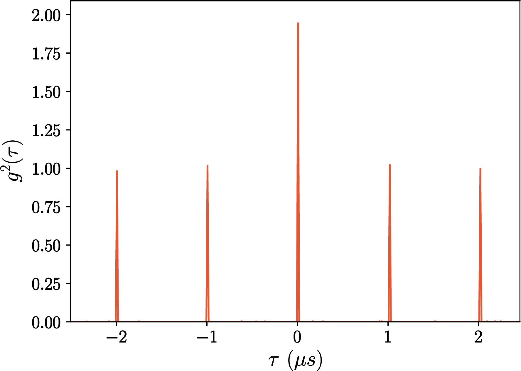
Referencing Fig. 3 in the main manuscript, the phase and amplitude modulations required to reproduce the correct P-function of a thermal state were provided via the two electro-optic modulators (EOMs) fibre-coupled to the laser source (a vertical cavity surface-emitting laser (VCSEL)). A dual-channel arbitrary waveform generator provided independent electrical driving voltages to the EOMs which in turn applied a variable phase and amplitude modulation onto the individual coherent states generated by the VCSEL. Both modulators were LiNbO3 based with low insertion and coupling loss ( dB) and low DC control voltages ( V for phase inversion). The amplitude modulators comprised two laser inscribed waveguides configured in a Mach-Zehnder pattern where an external RF signal would change locally the refractive index of one arm actively altering the output power of the device. In order to reduce any external interference during their operation, the EOMs were mechanically and thermally isolated from the environment enhancing their operational stability. The final pseudo thermal source was tested by means of a Hanbury Brown and Twiss like experiment Brown and Twiss 1956 were second order correlations between the two detectors monitoring the interferometer were measured for different time delays via the Qucoa analysis software for the HydraHarp 400 (PicoQuant) TCSPC module. Fig. S2 shows the computed as a function of the time delay between detectors DA and DB for a pulsed source with a repetition rate of 1 MHz. The results showed a maximum at zero delay of , in close agreement with the theoretical value of a true thermal source.
VIII Interferometric calibration
The experimental set-up depicted in Fig. 3 in the main manuscript, relied on spatial mode sorting of the pseudo thermal states via interferometric means. However, precise and reliable control over the optical path difference of the device was paramount for the desired sorting operation. Therefore, we implemented an active feedback loop mechanism to have direct control over the interferometer and the relative phase difference of its inputs. A reference coherent signal was multiplexed into the input signals via the same EOMs used for the generation of the pseudo thermal states. This mechanism effectively halved the final repetition rate to 500 KHz since every two laser pulses, one was used for calibration and tuning operations. Fig. S3 depicts a simplified representation of a one-shot modulation signal used for the phase changing EOM. The first signal applies a voltage that imprints a complete shift onto the coherent state while the second signal applies a random phase uniformly extracted from the set ensuring that the final P-function was not skewed due to limited randomness generation Zanforlin et al. 2019; Marangon et al. 2016. The adjustable air-gap placed in one of the optical path of the interferometer was then used to ensure that the phase applied to the reference signal state was kept constant throughout the detectors’ integration time thus resulting in high interferometric visibility ().

IX Optical mask fabrication and characterization
The optical masks were formed using patterned etching of thin chromium layers on a fused silica substrate. The 1.5 mm thick fused silica substrates were coated with 90 nm thickness of chromium using an electron-beam vacuum evaporation process forming a layer sufficiently thick to be fully opaque to the near-infrared radiation used in this experiment. The substrate was then coated in 5 nm positive photoresist (AZ 1505), and the pattern (pinholes, reference and alignment markers) inscribed using a Heidelberg DW66+ laser-writer. Once developed, the chromium was removed using a chemical etchant (TechniEtch Cr01). Fig. S4 displays pictures of the masks taken with a Leica DMRM microscope (15x magnification).

A single-photon sensitive CCD camera (Rolera EM-C2 Bio-Imaging Microscopy Camera) was used to extract profile intensity images of the transmitted light by the two circular pinholes at different distances. Fig. S5 shows the normalised intensities at imaging distances and 20 cm for a mask with 30 m wide pinholes separated by 1 mm using thermal radiation. At short distances, the intensity profiles depict the classical Airy diffraction pattern expected from circular apertures where faint secondary rings are visible. In these configurations, the two sources can still be resolved, however, as the distance between the masks and the camera increases, diffraction prevails and the profiles merge together removing any knowledge of the initial sources.

The masks were also tested using coherent radiation to ensure that the thermal generation process successfully removed any spatial correlation that could potentially disrupt the interferometer’s mode sorting mechanism. Fig. S6 shows the resulting image for a mask with 30 m wide pinholes separated by 150 m placed at a distance cm from the camera. Interferometric fringes are clearly recognizable showing a fringe separation of mm which is in good agreement with the theoretical value expected for this imaging system.

X Quantum state discrimination
In a previous work Lupo et al. 2020, we have shown that a two-mode interferometer has the same sensitivity in estimating the separation between two sources as SPADE, given comparable numerical apertures. Here we show that the same two-mode interferometer is also optimal in our discrimination problem here.

Consider the set-up in Fig. S7 where two collectors are places at positions and orthogonal to the optic axis; the collectors are at a distance from the sources. One source (the star) is positioned at , and the planet, if present, is positioned at . Assuming we are in the paraxial regime, the optical path difference of the planet between the two collectors is is
| (S2) |
The optical path difference of the star to the two collector is
| (S3) |
The states to discriminate between are
| (S4) |
We redefine the angular separation . In the basis of , the two density matrices are
| (S9) |
The relative entropy between and is approximately
| (S10) |
Now, we apply the measurement in Fig. S7. We put the collected light at through a phase shift , followed by a 50:50 BS. We assume the operators transform as
| (S11) |
For , the measurement outcomes are
| (S12) |
For , they are
Define
| (S14) |
We set to
| (S15) |
This is analogous to the SPADE method, where we align the apparatus to the weighted center. That is, this step assumes that we know the centre-of-mass of the two sources. If the planet is absent, then this is equal to the position of the star.
The classical relative entropy of this measurement is
| (S16) |
which is optimal in the limit that (see Supp. Material).
XI Angular separation estimation
XI.1 The reference laser
In the experiment, the laser is input into a multimode fibre, goes through free space (sprays out like a spherical point source), and then comes through the two slits. Since there is no randomness introduced in the process, we model the output at the two slits as a plane wave of coherent states. The reference laser provides a calibration for the applied phase .

The electric field at is given by the combination of the two fields of the two souces
The photon numbers at and are:
The optical path differences are
| (S19) |
Since the two slits are of the same size (equal intensity), we model the coherent states at and as
We need to calculate the expectation value of this observable to obtain the correlations:
| (S20) |
The expectation value of the operator in Eq. (XI.1) is
| (S21) |
After the collectors ate and , we have a phase-shifter and 50:50 beam splitter. This transformation gives
| (S22) |
We can now calculate the statistics of the coherent state at the two detectors, and . Inversing the above gives
| (S23) |
If the interferometer is imperfect, where some of the signal is replaced by noise, we model this as
| (S24) |
If we were to compute the difference in photon counts between the two detectors, we find that
| (S25) |
For , which is our case here, since the two slits are equidistant from the output of the multimode fibre, the above expression reduces to . That is, the reference laser behaves almost like a single point source. The parameter being non-zero will only reduce the visibility of the measurement, and the effect is almost neglible.
We measure the parameter directly from experimental data, which is then used to update the probability distribution in the maximum likelihood method.
XI.2 Maximum likelihood
In our analysis, we use a maximum likelihood method to obtain an estimator. Using Eq. 11 in the main text, we can estimate by the estimator , then obtain from
| (S26) |
We can use maximum likelihood method to obtain via Baye’s theorem. Therefore, we would like to obtain the probability distribution for , given the detection events, and . For two events and , Baye’s theorem states that
| (S27) |
Initially the probability distribution for is uniform in , therefore . After one detection event and adjustable phase , we have
| (S28) |
Here there is a normalisation factor that can be fixed ‘easily’. We know , these are
| (S29) |
Given a detection event where the adjusted phase was , the probability for can be updated via
| (S30) |
Therefore, after the detection event, Eq. (S30) is updated using Eq. (XI.2), depending on whether or occurred. After detection events, we have the vector of deteciton events, e.g. , given a vector of adjustable phases . In the experiment, is constant for each data point.
We have
| (S31) |
Now, since all the functions we deal with here are sinusoid, we can conveniently express them as a Fourier series. After clicks, the probabilities can be expressed as a Fourier series
| (S32) |
where here corresponds to the higher order of the Fourier coefficient. The coefficient of the term is denoted , which depends on and . Normalising to will keep the entire distribution normalised.
We equivalently write the update events in this Fourier form. For example, if detector fires, then
| (S33) |
We write Eq. (S33) as
| (S34) |
therefore the update coefficients are . This example is particularly relevant, because the factor is equal to in Eq. (XI.1), and is directly measured in the experiment using the calibration laser.
Before the first detection, Eq. (S32) only contains one term, . After each detection event given by the probabilities in Eq. (XI.2), the number of Fourier coefficients grow by 2; are updated using Eq. (S31), which once again uses Eq. (XI.2).
After the coefficients are obtained, can be evaluated for each value of , and we extract the maximum. There are two peaks for of equal intensity, since We show a simulated example in Fig. S9, we use the parameter ; after 10000 detection events where were were output at detector .