Distributed Transient Safety Verification via Robust Control Invariant Sets: A Microgrid Application
Abstract
Modern safety-critical energy infrastructures are increasingly operated in a hierarchical and modular control framework which allows for limited data exchange between the modules. In this context, it is important for each module to synthesize and communicate constraints on the values of exchanged information in order to assure system-wide safety. To ensure transient safety in inverter-based microgrids, we develop a set invariance-based distributed safety verification algorithm for each inverter module. Applying Nagumo’s invariance condition, we construct a robust polynomial optimization problem to jointly search for safety-admissible set of control set-points and design parameters, under allowable disturbances from neighbors. We use sum-of-squares (SOS) programming to solve the verification problem and we perform numerical simulations using grid-forming inverters to illustrate the algorithm.
I Introduction
The massive failure of the Texas electrical grid in February 2021 [1] gave global coverage to the issue of power network resilience. During these extreme events, time and resources are of essence for the grid operator to assess the situation and take appropriate actions to maintain the operating state of the power network. Hence, to an extent it is imperative on the grid operator to be prepared for extreme events. Microgrids, both grid-connected and stand-alone, have shown promise to enhance resilience and reliability by paving a way of coordinating multiple distributed energy resources (DERs) as a locally operated single controllable entity [2, 3]. However, ensuring operational stability, safety, and reliability of any power network involves a complex multi-timescales problem, spanning sub-seconds to minutes and hours. Traditional power system control operations were largely structured around a temporal decoupling which allows slower-timescale operations (e.g., optimal dispatch) need not directly take into account faster-timescale constraints, and vice versa. However, with the emergence of inverter-based DERs and the associated changes in power systems dynamics (e.g., reducing inertia), the timescales separation is expected to continue to shrink [4]. The droop-controlled inverter based microgrids have a lower inertia than conventional generators, which allows large variations of the voltage and frequency of each inverters [3, 5]. The fluctuations happen during the transient evolution occurring as a result of a fault or due to the transitions between the power set-points, and can lead to violation of safety constraints [6]. It is imperative to develop a mechanism to inform slower-timescale operations (e.g., optimal dispatch of power set-points) of the constraints arising from faster-timescale (transient) dynamics.
Many recent efforts have addressed this need via, for example, stability and security-constrained optimization [7, 3, 5], identification of local and distributed parametric stability conditions [6, 8, 9], etc. The distributed identification of stability conditions are particularly interesting since these fit well into a multi-ownership models of microgrid resources, and facilitate hierarchical and plug-and-play operations [10]. However, most of the related literature, as above, only focus on the stability which concerns with the convergence of power system trajectories (close) to its normal operating point after a disturbance. The concept of safety, on the other hand, relates to avoiding critical operational limits (e.g., on voltages and frequencies), even under large disturbances. Safety is closely tied to resilience, since often in cyber-physical adversarial scenarios, an immediate priority is to contain the system trajectories within some acceptable set, rather than ensuring return to normality.
Safety-constrained control techniques are gaining recent attention in the power systems community [11, 12, 13, 14]. Model-predictive control [15] remains one of the most commonly used methods for enforcing dynamic constraints over some prediction horizon. However, it suffers from certain limitations in the context of power system dynamics, related to, for example, nonlinearity and associated complexity of the dynamics, information disparity due to communication overheads and/or privacy concerns, and computational burden, especially for longer prediction horizon [13]. To circumvent these issues, distributed safety verification and control methods based on robust forward set-invariance principles have been proposed in [11, 12, 13, 14]. However, these prior works rely on the existence or the construction of parametric Lyapunov functions and/or barrier functions, thereby often incurring prohibitive computational costs and resulting in conservative safety certificates. The work in [11], for example, proposes a sum-of-squares (SOS) programming based computation algorithm for distributed safety certificates as a super-level set of barrier functions. However, such computational methods result in conservative estimates of the safety-guaranteed set (e.g., Fig. 1 in [11]), and typically do not scale well.
In this work, we consider a hierarchical and modular microgrid control architecture, [10, 14, 16], which allows system-level dispatch of power set-points to inverter-based resources, accommodating only limited data exchange between the (neighboring) inverter modules. Our objective is to design bounds on dispatched control set-points at the inverter buses, that guarantee, in a distributed sense, the safe excursions of local voltage and frequency within the specified limits while tolerating uncertainty in the neighboring buses. Specifically, the work presented in this paper relies on the Nagumo’s theorem [17, 18] to build an efficient method for distributed and robust safety verification, without requiring existence or construction of barrier functions. Thus, the proposed approach requires less computation, and relaxes the conservativeness of the barrier-certified safe sets by directly accommodating the original safety specifications. The explicit reference governor [19] relies on the same concept but we focus on establishing safe bounds on control inputs, instead of deriving a specific control law, which is the role of the grid coordinator [14].
The main contributions of this article are threefold. Firstly, we determine the maximal interval (bounds) of the dispatched control set-points guaranteeing the safety of droop-controlled inverters. Secondly, we establish the monotonic relationship between this interval of safety admissible control set-points and the droop coefficients. Finally, we calculate efficiently the maximal droop coefficient for which these safety admissible controls exist. As such, this paper provides novel design guidelines for the droop control parameters, extending the literature on stability-informed droop settings, e.g., [6, 8, 9], and the references therein. We use SOS programming to solve the safety verification problems, and illustrate the algorithm via numerical simulations. The remainder of this article is structured as follows. Section II provides a background of the relevant theory. Section III presents our microgrid problem of interest. Section IV explains the theoretical approach which we illustrate on a numerical example in Section V. We conclude this article with Section VI.
II Preliminaries
II-A Invariant Sets
Consider a nonlinear dynamical system of the form
| (1) |
with a Lipschitz continuous function. The objective of our work is to identify safe sets that the state cannot leave. Such sets are called invariant (or positively invariant); we define them as in [18].
Definition 1
A set is invariant by the dynamics (1) if yields for all .
To characterize invariant sets we will be using a theorem first established by Nagumo [17] and then independently rediscovered by Brezis [20]. We state here a more modern formulation of this result from [18].
Theorem 1 (Nagumo 1942)
A closed set is invariant by the dynamics (1) if and only if for all , , with the Bouligand tangent cone to at .
A full definition of the Bouligand tangent cone is given in [18], but we will be studying sets where the Bouligand tangent cone is or . The geometrical interpretation of Nagumo’s theorem is that pointing inside on its boundary prevents trajectories from leaving .
II-B Network Safety
In a network, the dynamics of node can be modeled by
| (2) |
with a control input, an external input, and and their respective admissible sets. For such a system we need to adapt our definition of invariant sets following [18].
Definition 2
A set is robust control invariant by the dynamics (2) if there exists a feedback control law such that for all and all time-varying , for all .
We then want to determine the set of control inputs ensuring the robust control invariance of a given safe set despite the fluctuations in the neighboring inverter states. In particular, specific to the example of inverter-based microgrids, i.e., when the safe sets are expressed as box constraints on the states (as in (6)), we define the following:
Definition 3
A 1-dimensional set is upper invariant (resp. lower invariant) for a set of controls by the dynamics (2) if for all time-varying , and all , then for .
If is upper invariant (resp. lower invariant), then the state cannot escape by crossing the upper bound (resp. lower bound) of . Notice that if there are controls making both upper and lower invariant, then is a robust control invariant set. We denote such controls as safety admissible.
Definition 4
A set of controls is safety admissible for the set if for all controls , the set is robust control invariant.
As we will detail later, if the dynamics (2) and the safe set are polynomial, e.g., with polynomials, then the invariance condition of Nagumo’s theorem can be stated as a polynomial inequality, enabling its fast computation.
III Problem Description
A microgrid power network is operated by a microgrid coordinator that determines power setpoints for each node of the grid [14, 16]. The transition in between these setpoints, corresponding to a transient regime, might lead the frequency or voltage of some inverters to violate safety constraints. We are thus interested in ensuring the transient safety of microgrid networks, so that they are reliable when operated. Consider the case of droop-controlled inverters [6]:
| (3a) | ||||
| (3b) | ||||
| (3c) | ||||
where , and are, respectively, the phase angle, frequency and voltage magnitude of node . The droop-coefficients and are associated with the active power vs. frequency and the reactive power vs. voltage droop curves, respectively. The time-constant of the low-pass filter used for the active and reactive power measurements is . The nominal voltage magnitude is . The active power and reactive power set-points are and , respectively. Finally, the active and reactive power injected into the network are and , respectively following the nonlinear coupling equations
| (4a) | ||||
| (4b) | ||||
where , and is the set of neighbor nodes with the convention that . The transfer conductance and susceptance of the line connecting nodes and are denoted by and , respectively.
We use the formulation of [11] to model the capability of the inverters to change their control set-points of the active and reactive power output in order to adjust to different operating conditions. More specifically, we write
| (5) |
where and are the set-points for the nominal operating conditions; and and are control inputs. We are thus interested in maintaining at all times both voltage and frequency within some pre-specified safety limits. By a usual abuse of notation, instead of considering the actual voltage, we consider its difference from the nominal voltage p.u.. Following [11, 21, 22], we consider the voltage and frequency safe sets to be
| (6a) | ||||
| (6b) | ||||
For the inverters (3), the perturbation from Definition 2 are the neighbor voltage magnitudes () and phase angle differences () that determine the power transfers, and . For the purpose of this paper, we assume that the phase angle differences between (any) two neighbor buses are bounded as follows:
| (7) |
Note that such range of phase angle differences are typical of distribution feeders, and especially microgrids, that are often characterized by relatively short lines connecting two buses [23]. Furthermore, note that only the difference of phase angles and as opposed to their individual values, determine the power-flow connecting the nodes and . Thus, for simplicity to notations and without any loss of generality, we set as the reference angle, and use throughout this text. Then, we want to determine controls that maintain and , whatever the values of and for the neighbors .
Problem 1
(Safety-Admissible Control) What values of control set-points ensure that and are robust control invariant by the dynamics (3)?
Moreover, note that the impact of neighbor (and network) disturbances on the inverter dynamics (3) are enhanced by larger droop values, a fact which suggests the existence and size of the safety-admissible controls depend on the chosen droop coefficients. This motivates the following question:
Problem 2
(Maximal Droop) What values of droop coefficients ensure the existence of a non-empty safety-admissible set of controls, guaranteeing robust control invariance of and as per dynamics (3)?
IV Theoretical Construction
In this section we establish the theory concerning robust control invariant sets for droop-controlled inverters. Since and in the inverter dynamics (3), we can define a minimal lower control and a maximal upper control such that
If , then the maximal interval of safety admissible controls is . To illustrate these definitions and our objective let us study a simplified version of (3).
IV-A Simple Example
Consider the frequency dynamics equation (3b) when the inverter has a single neighbor. To simplify take s, rad/s/p.u., rad, p.u., p.u.-1 and a safe set Hz. Then, .
To make upper invariant, according to Nagumo’s theorem we need when . Thus, we want , so . We are looking for robust controls working for all possible . Then, the maximal upper control is , because for , we need .
Similarly, to make lower invariant, we need when . Then, we want , i.e., . Thus, the minimal lower control is .
In this setting, , there are no safety admissible controls making robust control invariant. A reason for this failure is that is too large, making unstable. Indeed, for small values of , (3b) can be approximated by which is stable. We will elaborate further on this issue in the following subsections.
IV-B Minimal controls for upper and lower invariance
Let us determine the minimal lower control for . By definition, . With (3b), . Then, the minimal that is larger than all is in fact the maximum of this term over all and , because is continuous in according to (4a) and, and are compact. Thus,
| (8) | ||||
Then, when and for all and , which guarantees lower invariance according to Nagumo’s theorem. Similarly, the maximal upper control is defined as
| (9) | ||||
and makes when and for all and . The minimal lower control and maximal upper control for the voltage equation are defined similarly.
A great way to solve the optimization problems (8) and (9) is to use a sum-of-squares (SOS) optimization. A multivariate polynomial , , is an SOS if there exist polynomial functions , such that . However, the power-flow equations (4) are not polynomials. Following [11] we choose a third order Taylor expansion of the dynamics (4) to make (3) polynomial. Then, (8) and (9) can be solved with any SOS tool.
IV-C Maximal droop for robust control invariance
The stability of the voltage and frequency rely on small droop coefficients . As in Section IV-A, when increases in (3), the perturbations and increase, and we thus have the intuition that the set of safety admissible controls should shrink. We can actually prove a stronger result by using the fact that the optimizations in (8) and (9) only affect .
Proposition 1
The bounds of the interval of safety admissible controls for and are inversely proportional to the droop coefficient .
Proof:
We first introduce the maximum and minimum of the active and reactive powers (4) at the lower and upper bounds of and . More specifically
| (10) |
A similar result holds for the voltage. ∎
Building on this result, we can then establish a sufficient condition for the existence of safety admissible controls.
Proposition 2
If the safe set contains in its interior, then safety admissible controls exist for some droop coefficients.
Proof:
Note that does not intervene in (4a), so the constraints for and are the same, which leads to . Then, based on (10), the condition is necessary and sufficient to make for small enough.
On the other hand, since intervenes in (4b), we cannot order and without computing them. Thus the condition is sufficient but maybe not necessary to make for some . ∎
Then, the safe sets of (6) guarantee that safety admissible controls exist for some small enough droop coefficients. We now want to find the maximal droop coefficient for which safety admissible controls exist, i.e.,
| (11) |
Remark 1
According to Proposition 1 and 2, if is in the interior of and , then the interval is not empty, is proportional with and makes robust control invariant,.
Proposition 3
The maximal droop coefficient is
| (12) |
Proof:
Since and are continuous in according to (10), definition (11) leads to . Using (10) we easily obtain the announced expression for . The calculation of is similar. ∎
The term in the denominator validates our intuition that increasing the range of possible perturbations decreases . The larger is, the larger can be, and thus the stronger the stabilizing term is in (3b), which increases . The same analysis holds for .
Remark 2
There are now two approaches to answer Problem 1 based on the controls and . If , then and any control in between guarantees the robust control invariance of the safe set. On the other hand, if we need a state-dependent control law. When the state gets too close from the upper (resp. lower) bound of its safe set, applying (resp. ) prevents safety violation. Besides, and can be precomputed, so that the sole real-time action of the controller is to decide which one of the controls to apply.
V Numerical Analysis
In this section we apply our theory to a modified microgrid model [24], and demonstrate the robust control invariance of the safe sets and introduced in (6). As per the modifications in [11, 14], four inverters were placed in the network, three of those at buses 1, 4, and 5, and the fourth at bus 0 after disconnecting the utility for islanded operation.
In a microgrid, the distance between inverters is small and thus the states of neighbors are strongly coupled. To account for this physical phenomenon we introduce two constants and measuring the range of allowable uncertainty of neighboring inverters such that and for . For the numerical analysis we choose p.u., which is of the nominal voltage , and Hz, which is of the Hz range of . The nominal droop coefficients of the network are rad/s/p.u. and p.u./p.u..
The coupling adds a constraint to the calculation of and . For instance, subject to , , for . We compute , with an SOS algorithm and we use the calculations of Proposition 1 to represent and on Figure 1.


As proven in Proposition 2, since is in the interior of , we were able to find values of for which safety admissible controls exist. On Figure 1, is located at the intersection of the green dash-dot lines representing and . Figure 2 shows that the same is true for . The computed values of are gathered in Table I.
| Inverter | 1 | 2 | 3 | 4 |
|---|---|---|---|---|
| [rad/s/p.u.] | ||||
| [p.u./p.u.] |
Note that for the voltage ranges from to of the nominal depending on the inverter. For the frequency, ranges from to of the nominal .
We now study how the admissible range of states , and impact the maximal droop coefficient .

In Figures 3 and 4, p.u. depicts a lack of coupling between inverters, because the length of is at most p.u., while for p.u. the coupling is perfect, i.e., for .
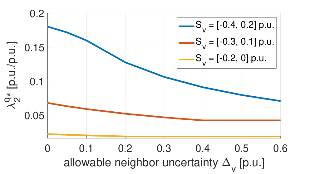
As predicted with (12) and illustrated on Figures 3 and 4, as the uncertainty ranges and increase, the value of decreases. The impact of the length of on is more difficult to predict as it affects both the numerator and denominator of in (12). However, the verdict of Figure 4 is clear: enlarging increases , the voltage has more wiggle room inside its safe set, it is thus easier to maintain .
We compute the controls and on an Intel Core i7-4770S with a CPU at 3.1GHz and 8GB of RAM. Previous works [11, 8] relied on the widely used MATLAB toolbox SOSTOOLS [25] and the semi-definite programming (SDP) solver SeDuMi [26]. However, the computation times were often excessive for nodes with more than two neighbors. We thus consider the Julia language [27], its SOS toolbox [28] and the SDP solvers SDPA [29] and Mosek [30]. As expected, Julia is faster and the computation times can be reduced by two orders of magnitude as shown on Table II.
| Language | MATLAB | Julia | Julia |
|---|---|---|---|
| SDP solver | SeDuMi | SDPA | Mosek |
| Run-time for and | 4295s | 343s | 33s |
In order to illustrate the invariance of the safe sets with the safety admissible controls calculated, we simulate the evolution of the voltage and the frequency of node 1. We use the original non-polynomial dynamics of the system. We choose and at respectively and of their nominal values, so that and . Then, the intervals of safety admissible controls are p.u. and p.u..
Every second we randomly choose a control value and as shown on Figures 5(5(a)) and 5(5(b)). Similarly, the states and of the neighboring nodes are stochastically updated every ms as depicted on Figures 5(5(c)) and 5(5(d)). The evolution of the voltage and frequency of node 1 are then pictured on Figures 5(5(e)) and 5(5(f)).


We can see that even randomly chosen controls, as long as they are within the safety admissible interval, enforce the safety of the system as and despite the stochastic variations of the neighbor states.
One could rightfully object that the stochastic nature of the variations of the neighbor states and prevent significant changes in and that could lead to safety violations. To overcome this limitation, we run a similar simulation where the neighbor states take their worst case values. To keep a constant phase angle rad, we need a constant frequency Hz and thus the frequency coupling must be removed by taking . We set the voltage at its lowest admissible bound, i.e., . We keep the same stochastic controls and same values of droop coefficients.
Figure 6(6(a)) shows how the voltage of a neighboring inverter follows its admissible lower bound. As illustrated on Figure 6(6(b)) and 6(6(c)) the voltage is maintained in and the frequency is maintained in despite the stochastic safety admissible controls and the lower bound neighbor states. Similar results are obtained when choosing at its upper bound and/or at its upper bound .


VI Conclusion and Future Work
In this paper we considered the problem of transient safety in inverter-based microgrids. Relying on Nagumo’s theorem, we developed two approaches to enforce the invariance of frequency and voltage sets of droop-controlled inverters. We solved the resulting optimization problems with SOS algorithms and successfully illustrated the safety methods on a microgrid model.
There are three promising avenues of future work. We first want to compare the efficiency of our approach in terms of size of invariant set and of computation times with barrier function and explicit governor approaches. We believe that a similar method can be used to handle safe energy storage, with only adding a state of charge constraint to the problem. Finally, we want to demonstrate our approach in conjunction with system level optimal dispatch problem.
Acknowledgment
This research was supported by the Resilience through Data-driven Intelligently-Designed Control (RD2C) Initiative, under the Laboratory Directed Research and Development (LDRD) Program at Pacific Northwest National Laboratory (PNNL). PNNL is a multi-program national laboratory operated for the U.S. Department of Energy (DOE) by Battelle Memorial Institute under Contract No. DE-AC05-76RL01830.
References
- [1] J. W. Busby, K. Baker, M. D. Bazilian, A. Q. Gilbert, E. Grubert, V. Rai, J. D. Rhodes, S. Shidore, C. A. Smith, and M. E. Webber, “Cascading risks: Understanding the 2021 winter blackout in Texas,” Energy Research & Social Science, vol. 77, pp. 1 – 10, 2021.
- [2] M. Farrokhabadi, C. A. Cañizares, J. W. Simpson-Porco, E. Nasr, L. Fan, P. A. Mendoza-Araya, R. Tonkoski, U. Tamrakar, N. Hatziargyriou, D. Lagos et al., “Microgrid stability definitions, analysis, and examples,” IEEE Transactions on Power Systems, vol. 35, no. 1, pp. 13–29, 2019.
- [3] Y. Xu, C.-C. Liu, K. P. Schneider, F. K. Tuffner, and D. T. Ton, “Microgrids for service restoration to critical load in a resilient distribution system,” IEEE Transactions on Smart Grid, vol. 9, no. 1, pp. 426 – 437, 2016.
- [4] J. A. Taylor, S. V. Dhople, and D. S. Callaway, “Power systems without fuel,” Renewable and Sustainable Energy Reviews, vol. 57, pp. 1322 – 1336, 2016.
- [5] A. Maulik and D. Das, “Stability constrained economic operation of islanded droop-controlled DC microgrids,” IEEE Transactions on Sustainable Energy, vol. 10, no. 2, pp. 569 – 578, 2018.
- [6] J. Schiffer, R. Ortega, A. Astolfi, J. Raisch, and T. Sezi, “Conditions for stability of droop-controlled inverter-based microgrids,” Automatica, vol. 50, no. 10, pp. 2457 – 2469, 2014.
- [7] E. Barklund, N. Pogaku, M. Prodanovic, C. Hernandez-Aramburo, and T. C. Green, “Energy management in autonomous microgrid using stability-constrained droop control of inverters,” IEEE Transactions on Power Electronics, vol. 23, no. 5, pp. 2346 – 2352, 2008.
- [8] S. Kundu, W. Du, S. P. Nandanoori, F. Tuffner, and K. Schneider, “Identifying parameter space for robust stability in nonlinear networks: A microgrid application,” in American Control Conference. IEEE, 2019, pp. 3111 – 3116.
- [9] S. P. Nandanoori, S. Kundu, W. Du, F. K. Tuffner, and K. P. Schneider, “Distributed small-signal stability conditions for inverter-based unbalanced microgrids,” IEEE Transactions on Power Systems, vol. 35, no. 5, pp. 3981 – 3990, 2020.
- [10] J. M. Guerrero, J. C. Vasquez, J. Matas, L. G. De Vicuña, and M. Castilla, “Hierarchical control of droop-controlled ac and dc microgrids—a general approach toward standardization,” IEEE Transactions on Industrial Electronics, vol. 58, no. 1, pp. 158–172, 2010.
- [11] S. Kundu, S. Geng, S. P. Nandanoori, I. A. Hiskens, and K. Kalsi, “Distributed barrier certificates for safe operation of inverter-based microgrids,” in American Control Conference. IEEE, 2019, pp. 1042 – 1047.
- [12] Y. Chen, J. Anderson, K. Kalsi, S. H. Low, and A. D. Ames, “Compositional set invariance in network systems with assume-guarantee contracts,” in American Control Conference. IEEE, 2019, pp. 1027–1034.
- [13] Y. Zhang and J. Cortés, “Distributed bilayered control for transient frequency safety and system stability in power grids,” IEEE Transactions on Control of Network Systems, vol. 7, no. 3, pp. 1476–1488, 2020.
- [14] S. Kundu and K. Kalsi, “Transient safety filter design for grid-forming inverters,” in American Control Conference. IEEE, 2020, pp. 1299 – 1304.
- [15] D. Q. Mayne, J. B. Rawlings, C. V. Rao, and P. O. Scokaert, “Constrained model predictive control: Stability and optimality,” Automatica, vol. 36, no. 6, pp. 789–814, 2000.
- [16] M. Almassalkhi, S. Brahma, N. Nazir, H. Ossareh, P. Racherla, S. Kundu, S. P. Nandanoori, T. Ramachandran, A. Singhal, D. Gayme et al., “Hierarchical, grid-aware, and economically optimal coordination of distributed energy resources in realistic distribution systems,” Energies, vol. 13, no. 23, p. 6399, 2020.
- [17] M. Nagumo, “Über die lage der integralkurven gewöhnlicher differentialgleichungen,” Proceedings of the Physico-Mathematical Society of Japan. 3rd Series, vol. 24, pp. 551 – 559, 1942.
- [18] F. Blanchini, “Set invariance in control,” Automatica, vol. 35, no. 11, pp. 1747 – 1767, 1999.
- [19] M. M. Nicotra and E. Garone, “The explicit reference governor: A general framework for the closed-form control of constrained nonlinear systems,” IEEE Control Systems Magazine, vol. 38, no. 4, pp. 89–107, 2018.
- [20] H. Brezis, “On a characterization of flow-invariant sets,” Communications on Pure and Applied Mathematics, vol. 23, no. 2, pp. 261 – 263, 1970.
- [21] K. P. Schneider, N. Radhakrishnan, Y. Tang, F. K. Tuffner, C.-C. Liu, J. Xie, and D. Ton, “Improving primary frequency response to support networked microgrid operations,” IEEE Transactions on Power Systems, vol. 34, no. 1, pp. 659 – 667, 2018.
- [22] J. Elizondo, R. Y. Zhang, P.-H. Huang, J. K. White, and J. L. Kirtley, “Inertial and frequency response of microgrids with induction motors,” in 17th Workshop on Control and Modeling for Power Electronics. IEEE, 2016, pp. 1 – 6.
- [23] W. H. Kersting, “Radial distribution test feeders,” IEEE Transactions on Power Systems, vol. 6, no. 3, pp. 975–985, 1991.
- [24] T. Ersal, C. Ahn, I. A. Hiskens, H. Peng, and J. L. Stein, “Impact of controlled plug-in evs on microgrids: A military microgrid example,” in Power and Energy Society General Meeting. IEEE, 2011, pp. 1–7.
- [25] A. Papachristodoulou, J. Anderson, G. Valmorbida, S. Prajna, P. Seiler, and P. A. Parrilo, SOSTOOLS: Sum of squares optimization toolbox for MATLAB, 2013, available from http://www.cds.caltech.edu/sostools.
- [26] J. F. Sturm, “Using SeDuMi 1.02, a MATLAB toolbox for optimization over symmetric cones,” Optimization Methods and Software, vol. 11, pp. 625 – 653, 1999, software available at http://fewcal.kub.nl/sturm/software/sedumi.html.
- [27] J. Bezanson, S. Karpinski, V. B. Shah, and A. Edelman, “Julia: A fast dynamic language for technical computing,” arXiv preprint arXiv:1209.5145, 2012.
- [28] B. Legat, C. Coey, R. Deits, J. Huchette, and A. Perry, “Sum-of-squares optimization in Julia,” in First Annual JuMP-dev Workshop, 2017.
- [29] M. Yamashita, K. Fujisawa, M. Fukuda, K. Kobayashi, K. Nakata, and M. Nakata, “Latest developments in the SDPA family for solving large-scale SDPs,” in Handbook on semidefinite, conic and polynomial optimization. Springer, 2012, pp. 687 – 713.
- [30] J. Dahl, “Semidefinite optimization using MOSEK,” in International Symposium on Mathematical Programming, 2012.