Unsupervised Multiple-Object Tracking
with a Dynamical Variational Autoencoder
Abstract
In this paper, we present an unsupervised probabilistic model and associated estimation algorithm for multi-object tracking (MOT) based on a dynamical variational autoencoder (DVAE), called DVAE-UMOT. The DVAE is a latent-variable deep generative model that can be seen as an extension of the variational autoencoder for the modeling of temporal sequences. It is included in DVAE-UMOT to model the objects’ dynamics, after being pre-trained on an unlabeled synthetic dataset of single-object trajectories. Then the distributions and parameters of DVAE-UMOT are estimated on each multi-object sequence to track using the principles of variational inference: Definition of an approximate posterior distribution of the latent variables and maximization of the corresponding evidence lower bound of the data likehood function. DVAE-UMOT is shown experimentally to compete well with and even surpass the performance of two state-of-the-art probabilistic MOT models. Code and data are publicly available.
Index Terms:
Unsupervised Learning, Dynamical Variational Autoencoder, Multiple Object Tracking, Probabilistic TrackingI Introduction
Multi-object tracking (MOT), or multi-target tracking, is a fundamental and very general pattern recognition task. Given an input time-series, the aim of MOT is to recover the trajectories of an unknown number of sources, that might appear and disappear at any point in time [1, 2]. There are four main challenges associated to MOT, namely: (i) extracting source observations (also called detections) at every time frame, (ii) modeling the dynamics of the sources’ movements, (iii) associating observations to sources consistently over time, and (iv) accounting for birth and death of source trajectories.
In computer vision, the tracking-by-detection paradigm has become extremely popular in the recent years [3, 4, 5, 2]. In this context, more and more powerful detection algorithms brought a significant increase of performance [6, 7, 8]. Including motion information also improves the tracking performance [9, 10, 11]. Among the tracking approaches based on motion models, the linear dynamical model (i.e., constant object velocity) is the most commonly used [12, 4, 10]. Further, it makes sense to combine the detection and tracking models together [10, 13, 14].
While a linear dynamical model is suitable in case of high sampling rate and reasonable object velocity, challenging tracking scenarios with low sampling rate, moving camera, high object velocity, rapid changes of direction, and occlusions are still difficult to tackle with such simple models, thus leading to numerous tracking errors such as false negatives and identity switches. Therefore, more sophisticated nonlinear models using recurrent neural networks (RNNs) to capture the motion information have been proposed [15, 9, 16, 17, 18, 19, 20, 21].
The powerful sequential modeling capabilities of RNNs can help to design more accurate motion models, provided we have enough annotated data to train them. Since obtaining annotations in the MOT framework is a very tedious and resource-consuming task, it is worth investigating the training of complex motion/MOT models in an unsupervised manner, i.e., without human-annotated data.
In the present paper, we propose a probabilistic unsupervised MOT model. We focus on challenges (ii) and (iii) above. First, we propose to use a dynamical variational autoencoder (DVAE) to model the complex motion patterns of each tracked object. DVAEs are a family of powerful deep probabilistic generative models with latent variables designed for modeling correlated sequences of (multidimensional) data [22]. They can be seen as a combination of the variational autoencoder (VAE) [23, 24] with recurrent neural networks (RNNs). The DVAE is pre-trained on a synthetic dataset of single-object trajectories generated without human annotations. This pre-training is done using the variational inference (VI) methodology, which is classical in the VAE context and consists of defining an approximate posterior distribution of the latent variables and maximizing a lower bound of the data likelihood function. Second, the DVAE is combined with an observation-to-object assignment latent variable to solve the MOT task – hence the name DVAE-UMOT. The distributions and parameters of the complete DVAE-UMOT model are estimated on each multi-object sequence to track, using again the VI methodology, which includes here the observation-to-object assignment and the estimation of objects position. Experiments conducted on a dataset derived from MOT17 (which is part of the MOTChallenge [25]) show that our model exhibits a very competitive tracking performance, even for long tracks of 300 frames, and can outperform two recent state-of-the-art MOT models (including a model that was trained using MOT17 annotations) on several MOT metrics.
The rest of this paper is organised as follows. We discuss the related work in Section II. The theoretical background of VI and DVAEs is introduced in Section III. The main developments of the proposed DVAE-UMOT model and algorithm are presented in Section IV and implementation details are provided in Section V. Experimental results and comparison with state-of-the-art approaches are presented and discussed in Section VI. We draw conclusions and discuss the future work in Section VII.
II Related Work
Motion models in MOT. In tracking-by-detection MOT algorithms, data association is usually done by extracting features from the video sequences, using them to compute a feature affinity matrix and finally use this matrix to assign detections to targets [5, 2]. A number of appearance models have enabled good tracking performance [26, 4, 27, 28, 29, 30]. However, models based on visual features only are less robust to similar appearances, occlusions and noisy detections. To solve this problem, several approaches combined motion features with appearance features to construct more robust MOT models. A Kalman filter was used in [4, 12, 10, 14] to exploit the motion information, assuming that the targets follow a linear dynamical model, i.e., they have a constant velocity, at least locally (on a portion of the trajectory). In [31], a Kalman filter was integrated into a VI framework so as to combine both audio-visual observations and a motion model together. Nevertheless, linear dynamical models only consider the temporal dependencies between adjacent frames and thus cannot deal efficiently with long-term occlusions.
With the spreading use of neural networks, more sophisticated nonlinear motion models have been developed. RNNs were used in [16] to mimic the classical Bayesian filtering state estimation. The authors of [15] proposed to combine multiple cues such as appearance, motion and interaction cues within an RNN architecture. In [9], RNNs were used to predict the targets motion and tracklet-stitching was used to handle occlusions. All these methods used RNNs for modeling nonlinear temporal dependencies. Still, the capabilities of deterministic RNNs remain limited for long sequences. A recurrent autoregressive network was used in [32] to extract long-term temporal dependencies and to learn a probabilistic generative model for multiple object trajectories. The authors of [11] proposed an RNN-based probabilistic autoregressive motion model which can be used to both score tracklet proposals and inpaint tracklets in case of occlusion. These works adopted a probabilistic point of view and constructed more flexible motion models. However, these motion models have not been combined with the MOT algorithm in a principled way. In our proposed model, we adopt a complete probabilistic perspective. We propose to use the DVAE models to capture the long-term temporal dependencies of object positions and combine them with an observation-to-object assignment variable within a VI framework. In addition to estimate the assignment probabilities, the proposed DVAE-UMOT model can also filter out detection noise to form smooth trajectories. The powerful sequential modeling capability of DVAEs guarantees the accuracy of long-term tracking.
Unsupervised MOT. Compared with the relatively large number of supervised MOT methods, unsupervised MOT methods are much less explored in the literature and differ a lot from one to another. The authors of [33] firstly grouped objects into short tracklets using their spatio-temporal consistency. And then long-term consistent tracks were formed based on the objects’ visual similarity, using a tracklet-based Forest Path Cutting data association algorithm. The authors of [34] followed a similar line, using a re-identification model trained with noisy-labeled data to extract the appearance features used to form the long-term tracks. Another branch of unsupervised models is based on geometric rendering and visual reconstruction. The authors of [35] proposed a tracking-by-animation framework, which first tracks objects from video frames and then renders tracker outputs into reconstructed frames. A VAE-based spatially-invariant label-free object tracking model was proposed in [36]. In their work, the VAE encoder, which takes as input the sequential images, consists of three modules: a discovery module to detect newly birthed objects, a propagation module to update the attributes of existing objects, and a selection module to select objects and deal with track death. The VAE decoder is a rendering module that reconstructs the video sequence. The model is trained in an unsupervised way without using manual annotations. In our proposed model, we focus on the dynamical modeling of objects in MOT. And we only exploit the motion information without using appearance features. In this context, the term unsupervised means that we do not use any manually annotated ground-truth object position sequence to train the model.
DVAE models. Firstly proposed in [23, 24], the VAE is a powerful deep probabilistic generative model which learns a low-dimensional latent space underlying the generation of high-dimensional complex data. It has been successfully applied in many different fields [37, 38, 39]. The original VAE model does not include sequential modeling. The DVAE models integrated RNNs into the VAE structure to build deep probabilistic generative models for sequential data [22]. Similar to the VAE, DVAE models are also based on an encoder/decoder structure, here with a sequence of latent variables associated to a sequence of observed data. As more largely discussed in Section III-B, different temporal dependencies between the observed and latent variables result in different DVAE models. DVAEs have been applied for different tasks, e.g., the disentanglement of speech factors of variation [40] and speech enhancement in noise [41]. We show in this paper that the DVAE models can also be successfully used for MOT. To our knowledge, this is the first time DVAEs are used for this task.
III Methodological Background
III-A Latent variable generative models and variational inference
The methodology of the proposed MOT algorithm lies under the very broad umbrella of latent variable generative models (LVGMs) and associated variational inference (VI) methodology [42, 43]. An LVGM depicts the relationship between an observed and a latent random (vector) variable from which is assumed to be generated. We consider an LVGM defined via a parametric joint probability distribution , where denotes the set of parameters. In a general manner, we are interested in two problems closely related to each other: 1) estimate the parameters that maximize the observed data (marginal) likelihood , and 2) derive the posterior distribution so as to infer the latent variable from the observation .
A prominent tool to estimate is the family of expectation-maximisation (EM) algorithms, that maximizes the following lower bound of the marginal likelihood, called the evidence lower-bound (ELBO):
| (1) |
where is a distribution on conditioned on . The EM algorithm is an iterative alternate optimisation procedure that maximizes the ELBO w.r.t. the distribution (E-step) and the parameters (M-step). Maximizing the ELBO w.r.t. is equivalent to minimising the Kullback-Leibler divergence (KLD) between and the exact posterior distribution [43]. When is computationally tractable, it is optimal to choose , then the ELBO is tight and the EM is called “exact.” Otherwise, the optimization w.r.t. is constrained within a given family of computationally tractable distributions and the bound is not tight anymore. We then have to step in the VI framework.
A first family of VI approaches is the structured mean-field method [44] which consists in splitting into a set of disjoint variables . The approximate posterior distribution is thus assumed to factorise over this set, i.e., , which leads to the following optimal factor, given the parameters computed at the previous M-step, :
| (2) |
Since each factor is expressed as a function of the others, this formula is iteratively applied in the E-step of the EM algorithm until some convergence criterion is met.
A second approach is to rely on amortised inference [45], where a set of shared parameters is used to compute the parameters of the approximate posterior distribution. A very well-known example is the variational autoencoder (VAE) [23, 24]. For a reason that will become clear in Section IV, let us here denote by the observed variable and by the latent one. In a VAE, the joint distribution is defined via the prior distribution on , generally chosen as the standard Gaussian distribution , and via the conditional distribution on , generally chosen as a Gaussian with diagonal covariance matrix . The mean and variance vectors and are nonlinear functions of provided by a deep neural network (DNN), called the decoder network, taking as input. is here the (amortized) set of parameters of the DNN. The posterior distribution corresponding to this model does not have an analytical expression and it is approximated by a Gaussian distribution with diagonal covariance matrix , where the mean and variance vectors and are non-linear functions of implemented by another DNN called the encoder network and parameterized by . The ELBO is here given by:
| (3) |
In practice, the ELBO is jointly optimized w.r.t. and using a combination of stochastic gradient descent (SGD) and sampling [23]. This is in contrast with the EM algorithm where and are optimized alternatively.
III-B From VAE to DVAE
In the VAE, each observed data vector is considered independently of the other data vectors. The dynamical variational autoencoders (DVAEs) are a class of models that extend and generalize the VAE to model sequences of data vectors correlated in time [22]. Roughly speaking, DVAE models combine a VAE with temporal models such as recurrent neural networks (RNNs) and/or state space models (SSMs). They can be used to model sequences of object bounding boxes/positions and are therefore suitable for MOT.
Let and be a discrete-time sequence of observed and latent vectors, respectively, and let denote the set of past observed and latent vectors at time . Using the chain rule, the most general DVAE generative distribution can be written as the following causal generative process:
| (4) |
where and are arbitrary generative distributions, which parameters are provided sequentially by RNNs taking the respective conditioning variables as inputs. A common choice is to use Gaussian distributions with diagonal covariance matrices:
| (5) |
| (6) |
It can be noted that the distribution of is more complex than the standard Gaussian used in the vanilla VAE. Also, the different models belonging to the DVAE class differ in the possible conditional independence assumptions that can be made in (4).
As for the VAE, the exact posterior distribution corresponding to the DVAE generative model is not analytically tractable. Again, an inference model is defined to approximate the exact posterior distribution and factorises as:
| (7) |
where denotes the set of past latent variables and all observations. Again, the Gaussian distribution with diagonal covariance matrix is generally used:
| (8) |
where the mean and variance vectors are provided by an RNN (the encoder network) taking as input and parameterized by . With the most general generative model defined in (4), the conditional distribution in (7) cannot be simplified. However, if conditional independence assumptions have been made in (4), the dependencies in might be simplified using the D-separation method [43, 46], see [22] for details. In addition, we can force the inference model to be causal by replacing with . This is particularly suitable for on-line processing. In the rest of the paper, we will use the causal inference model, i.e., in (7) and (8).
Similar to the VAE, and following the general VI principle, the DVAE model is also trained by maximizing the ELBO with a combination of SGD and sequential sampling. The ELBO has here the following general form [22]:
| (9) |
IV DVAE-UMOT Model and Algorithm
IV-A Problem formulation and notations
Let us consider a video sequence containing moving objects that we want to track over time. Let denote the object index and let be here the true (unknown) position vector of object at time frame . As commonly done in the computer vision community, we use a bounding box to characterize an object position, and is the coordinates vector of the top-left and bottom-right points of the bounding box that represents the true position of object . As our model follows the tracking-by-detection paradigm, the observations that we use here are the detected bounding boxes provided by a customized detector such as FRCNN [6]. Let us denote by the total number of detected bounding boxes at time frame , which can vary over time. We denote by , , the coordinates vector of the top-left and bottom-right points of the -th detected bounding box at frame .
The MOT problem consists in estimating the position vector sequence , for each object , from the complete set of observations . To solve this problem, we define two additional sets of latent variables. First, for each object at time frame , we define a latent variable , which is associated to through a DVAE model. This DVAE model, which is identical for all objects, is used to model the dynamics of each object in the analyzed video and plugged into the proposed MOT model. In a VAE or DVAE, the latent dimension is usually smaller than the dimension of the observed vector, in order to obtain a compact data representation. In the present work, the input dimension, which equals 4, is already small, so that we set the same dimension for ; that is, . Second, for each observation , we define a discrete observation-to-object assignment variable taking its value in . means that observation at time frame is assigned to object . This variable is used to form the tracklets. Each tracklet is a consistent object trajectory, i.e., a sequence of estimated position vectors consistent over time and assigned to the same object.
Hereinafter, to simplify the notations, we use “:” as a shortcut subscript for the set of all values of the corresponding index. For example, is the complete trajectory of object and is the set of position vectors for all objects at time frame . All notations are summarized in Table I.
| Variable notation | Definition |
|---|---|
| , | Sequence length and frame index |
| , | Total number of objects and object index |
| , | Number of observations at , and obs. index |
| True position of object at time | |
| Latent variable of object at time | |
| Observation at time | |
| Assignment of observation at time | |
| Position sequence of object | |
| Position of all objects at time | |
| Set of all object positions | |
| , , | Analogous for the latent variable |
| Set of all observations | |
| Set of all assignment variables |
IV-B General principle of the proposed solution
The general methodology of DVAE-UMOT is to define a parametric joint distribution of all variables , then estimate its parameters and (an approximation of) the corresponding posterior distribution , from which we can deduce an estimate of for each object . The proposed DVAE-UMOT generative model is presented in Section IV-C. As briefly stated above, it integrates the DVAE generative model (4)–(6) to model the objects dynamics and does not use any human-annotated data for training.
As it is usually the case in (D)VAE-based generative models, both the exact posterior distribution and the marginalisation of the joint distribution are analytically intractable. Therefore we cannot directly use an exact EM algorithm and we resort to VI. We propose the following strategy, inspired by the structured mean-field method that we summarized in Section III-A, with being here equal to . In Section IV-D, we define an approximate posterior distribution that partially factorizes over . As a parallel to the proposed DVAE-UMOT generative model integrating the DVAE generative model, this approximate DVAE-UMOT posterior distribution includes the DVAE inference model. Finally, in Section IV-E, we present an EM-like iterative algorithm for jointly deriving the terms of the inference model (other than the DVAE terms) and estimating the parameters of the complete DVAE-UMOT model (i.e., training this model), based on the maximization of the corresponding ELBO. As we will see, this training is done directly on each multi-object sequence to process (i.e., a test MOT sequence) and does not require previous supervised training with a labeled dataset of multi-object training sequences. It only requires to pre-train the DVAE model, which is done on a dataset of synthetic single-object sequences. This is possible because the DVAE is a single-object model, which is applied times in parallel in the proposed MOT algorithm to process an -object scene.
IV-C Generative model
In this section, we define the proposed DVAE-UMOT generative model; that is, we specify the joint distribution of observed and latent variables . We assume that the observation variable only depends on and , while the assignment variable is a priori independent of the other variables. Applying the chain rule and these conditional dependency assumptions, the joint distribution can be factorised as follows:
| (10) |
Observation model: We assume that the observations are conditionally independent through time and independent to each other, that is to say, at any time frame , the observation only depends on its corresponding assignment and position vector at the same time frame. The observation model can thus be factorised as:11 1 In this equation, we use and not , since the value of is not specified.
| (11) |
Given the value of the assignment variable, the distribution is modeled by a Gaussian distribution:
| (12) |
This choice is motivated by the fact that a detected bounding box is generally not very far from the corresponding true bounding box. In other words, is a noisy version of (assuming ). is the covariance matrix of the observation noise.
Assignment model: Similarly, we assume that, a priori, the assignment variables are independent across time and observations:
| (13) |
For each time frame and each observation , the assignment variable is assumed to follow a uniform prior distribution:
| (14) |
Dynamical model: Finally, is modeled with a DVAE. The different tracked objects are assumed to be independent of each other. This implies that in the present work we do not consider the interactions among objects during tracking. More complex tracking models including object interaction are beyond the scope of this paper. With this assumption, the joint distribution of all objects position and corresponding latent variable can be factorised across objects as:
| (15) |
where is the DVAE model defined in (4)–(6) and applied to and (defining ).22 2 Here we denote the DVAE parameters by instead of in (4) to differentiate the DVAE parameters from the other MOT model parameters. In this work, we assume that the dynamics of all objects are modeled with the same DVAE encoder and decoder.
Overall, the generative model parameters to be estimated are: (note that ).
IV-D Inference model
The exact posterior distribution corresponding to the generative model described in Section IV-C is neither analytically nor computationally tractable [22, 31]. Therefore, we propose the following factorised approximation that leads to a computationally tractable inference model:
| (16) |
where corresponds to the inference model of the DVAE and the optimal distributions and are derived below in the E-step of the DVAE-UMOT algorithm. Note that, the factorization (16) is inspired by the structured mean-field method [44], since we break the posterior dependency between and . However, we keep the dependency between and at inference time since it is the essence of the DVAE. In addition, we assume that the posterior distribution of the DVAE latent variable is independent for each tracked object, so that we have:
| (17) |
where is given by (7) and (8) applied to . This is coherent with the generative model, where we assumed that the dynamics of the various tracked objects are independent of each other.
IV-E DVAE-UMOT algorithm and solution
To derive the posterior distributions and and the parameters of all the other involved distributions, we cannot directly use the generic solution of the structured mean-field method (2) because (16) does not factorise in disjoint latent variable sets (in other words, in (16) is conditioned on and not on ). We thus have to go back to the fundamentals of VI and iteratively maximize the ELBO of the DVAE-MOT model defined by:
| (18) |
By injecting (10) and (16) into (18), we can develop as follows:
| (19) |
The ELBO maximization is done by alternatively and iteratively maximizing the different terms corresponding to the various posterior and generative distributions. In the EM terminology, this corresponds to the following E and M steps.
IV-E1 E-S step
We first consider the computation of the optimal posterior distribution . To this aim, we first select the terms in (19) that depend on (the other terms being considered as a constant in this part of the optimization):
| (20) | ||||
Let us define:
| (21) |
where is the appropriate normalisation constant. (20) rewrites:
| (22) |
where denotes the Kullback-Leibler divergence (KLD). Therefore, the optimal distribution is the one minimising the above KLD:
| (23) |
Since for any pair , the assignment variable follows a discrete posterior distribution, we can denote the corresponding probability values by:
| (24) |
These values will be computed in the E-W step below. The expectation with respect to in (23) can be calculated using these values. However, the expectation with respect to cannot be calculated in closed form. As usually done in the (D)VAE methodology, it is thus replaced by a Monte Carlo estimate using sampled sequences drawn from the DVAE inference model at the previous iteration (see Section V-B). Replacing the distributions in (23) with (11), (15), and (17), and calculating the expectations with respect to and , we find that factorises with respect to as follows:
| (25) |
Each of these factors corresponds to the posterior distribution of the position of the -th tracked object. Given (23) and the DVAE generative and inference models, we rapidly see that at a given time , the distribution over has non-linear dependencies w.r.t. the previous and current DVAE latent variables and the previous source positions . These non-linear dependencies impede to obtain an efficient closed-form solution. We resort to point sample estimates obtained using samples of and of , at the current iteration and . With these samples the posterior distribution is approximated with (the details can be found in Appendix A-A):
| (26) |
where each term of the product in is shown to be a Gaussian:
| (27) |
with covariance matrix and mean vector given by:
| (28) |
| (29) |
where and are simplified notations for and , respectively denoting the variance and mean vector provided by the DVAE decoder network for object at time frame . As we have to sample both and , we need to pay attention to the sampling order. This will be discussed in detail in Section V-B. Importantly, in practice, is used as the estimate of .
Eq. (29) shows that the estimated position vector for object is obtained by combining the observations , i.e., the detected object positions, and the mean position vector predicted by the DVAE generative model. The balance between these two terms depends on the assignment variables , the observation model covariance matrix and the position vector covariance matrix predicted by the DVAE generative model . Ideally, the model should be able to appropriately balance the importance of these two terms so as to optimally exploit both the observations and the DVAE predictions.
IV-E2 E-Z step
In the E-Z step, we consider the posterior distribution of the DVAE. This distribution is defined by (17), (7) and (8). In (19), the corresponding term is the third one, which we denote by and which factorises across objects as follows (see Appendix A-B):
| (30) |
with
| (31) |
Inside the expectation , we recognize the ELBO of the DVAE model defined in (9) and applied to object . This suggests the following strategy. Previously to and independently of the DVAE-UMOT algorithm, as briefly stated before, we pre-train the DVAE model on a dataset of synthetic single-object unlabeled sequences (this is detailed in Section VI-B). This is done only once, and the resulting DVAE is then plugged into the DVAE-UMOT algorithm to process multi-object sequences. This provides the E-Z step with very good initial values of the DVAE parameters , and . As for the following of the E-Z step, the expectation over in (31) is not analytically tractable. A Monte Carlo estimate is thus used instead, using samples of both and , similarly to what was done in the E-S step. Finally, SGD is used to maximize (the Monte Carlo estimate of) , jointly updating , and ; that is, we fine-tune the DVAE model within the DVAE-UMOT algorithm, using the observations . Note that in our experiments, we also consider the case where we neutralize the fine-tuning, i.e., we remove the E-Z step and use the DVAE model as provided by the pre-training phase.
IV-E3 E-W step
Thanks to the separation of from the two other latent variables in (16), the posterior distribution can be calculated in closed form by directly applying the optimal structured mean-field update equation (2) to our model. It can be shown that this is equivalent to maximizing (19) w.r.t. . We obtain (see Appendix A for details):
| (32) |
with
| (33) |
where
| (34) |
IV-E4 M step
As discussed in Section III, the maximization step generally consists in estimating the parameters of the generative model by maximizing the ELBO over . We recall that . In this work, the parameters of the DVAE decoder and are first estimated (offline) by the pre-training of the DVAE and then fine-tuned in the E-Z step, all this jointly with the parameters of the encoder . Therefore, in the M-step, we only need to estimate the observation model covariance matrices . In (19), only the first term depends on . Setting its derivative with respect to to zero, we obtain (see Appendix A for details):
| (35) |
In practice, it is difficult to obtain a reliable estimation using only a single observation. We address this issue in Section V-C.
V Algorithm Implementation
V-A DVAE-UMOT initialization
| Compute , with input and ; |
| Sample from ; |
| Compute and with input and ; |
| Compute and with input and ; |
| Sample from ; |
| Compute using (36); |
| Compute ; |
| Fine-tune the DVAE parameters {, , } by applying SGD on ; |
Before starting the EM iterations of the proposed DVAE-UMOT algorithm, we need to initialize the values of several parameters and variables. Theoretically, there is no preference in the order of the three E-steps. In practice however, we chose to follow the order E-W Step, E-Z Step, E-S Step, and finally M Step, for initialization convenience. Indeed, starting with the M Step or the E-S/E-Z steps, requires the initialization of the assignment variables , which poses a problem because we do not have any prior knowledge about them. Instead, starting with E-W requires the initialisation of the object bounding boxes and their covariance matrices through the sequence, as well as the observation covariance matrices.
The estimate of , , can be easily initialised over a short sequence by assuming that the object does not move too much. Indeed, the initial values of can be set to the value of the observed bounding box at the beginning of the sequence . While this strategy is very straightforward to implement, it is too simple for many tracking scenarios, especially for long sequences. We thus propose to split a long sequence into sub-sequences. For each sub-sequence, we initialise to the value at the beginning of the sub-sequence. After this initialisation, we run a few iterations of DVAE-UMOT over the sub-sequence, allowing us to have an estimate of the object bounding box at the end of the sub-sequence. This value will then be used to provide a constant initialisation for the next sub-sequence. At the end, all these initializations are concatenated, thus providing a piece-wise constant initialization for DVAE-UMOT over the entire long sequence. After computing the E-W step, a sequence of samples from the previous iteration is sent through the E-S/E-Z steps, and the same initialisation values are taken. The implementation details as well as the pseudo-code of this cascade initialization strategy are provided in Appendix B.
Finally, for the initialization of the observation model covariance matrices , see Section V-C. The covariance matrices of the object bounding boxes are initialized with the same values as .
V-B Sampling order
As already mentioned in Section IV-E1, we must pay attention to the sampling order of and when running the iterations of the E-S and E-Z steps. As indicated in the pseudo-code of Algorithm 1, in practice, the E-S and E-Z steps are processed jointly. We start with the initial position vector sequence and the initial mean position vector sequence . At any iteration of the E-Z and E-S steps, for each tracked object and each time frame , we sample in the following order:
- 1.
Compute the parameters and 33 3 and are shortcuts for and respectively. of the posterior distribution of using the DVAE encoder network with inputs sampled at the previous iteration and sampled at the current iteration. Then, sample from .
- 2.
Compute the parameters and 44 4 Analogous definitions hold. of the generative distribution of using the corresponding DVAE network with inputs and , both sampled at the current iteration.
- 3.
Note that with the above sampling order, the Monte Carlo estimate of the ELBO term maximized in the E-Z step (31) is given by (for object ):
| (36) |
The whole DVAE-UMOT algorithm, taking into account these practical aspects, is summarized in the form of pseudo-code in Algorithm 1.
V-C Variance estimation
In our experiments, we observed that the estimated values of both and in (29) increased very quickly with the DVAE-UMOT algorithm iterations. This caused instability and unbalance between these two terms, which finally conducted the whole model to diverge. To solve this problem, we set to a given fixed value, which is constant on the whole analyzed -frame sequence and not updated during the DVAE-UMOT iterations. Specifically, the diagonal of is set to , where is a factor lower than 1. In common terms, is set to a fraction of the (squared) size of the corresponding observation at frame 1. This turned out to stabilise the iteration process and finally led to very satisfying tracking results. The value of is a hyperparameter of the model and its influence is experimentally evaluated in Section VI-E.
VI Experiments
VI-A Choice of the DVAE model
We recall that the DVAE is a general class of models that differ by adopting different conditional independence assumptions for the generative distributions in the right-hand-side of (4). Seven DVAE models have been extensively discussed, and six of them have been benchmarked in the analysis-resynthesis task (on speech signals and 3D human motion data) in [22]. We chose to use here the stochastic recurrent neural network (SRNN) model initially proposed in [47], because it was shown to provide a very good trade-off between complexity and modeling power in [22]. The probabilistic dependencies of the SRNN generative model are defined as follows:
| (37) |
To perform online tracking, we propose to use the following causal SRNN inference model:
| (38) |
The SRNN generative model is implemented with a forward LSTM network, which embeds all the past information of the sequence . Then, a dense layer with the tanh activation function plus a linear layer provide the parameters . Similarly, the parameters are computed with two dense layers with tanh activation function plus a linear layer appended to the LSTM as well. The inference model shares the hidden variables of the forward LSTM network of the generative model and uses two dense layers with the tanh activation function plus a linear layer to compute the parameters . More implementation details can be found in Appendix C.
VI-B DVAE pre-training
VI-B1 Dataset
We generated synthetic bounding box trajectories, in the form of -frame sequences () of 4D vectors gathering the top-left and bottom-right bounding box 2D coordinates. To generate bounding boxes with reasonable size, we do not generate the four dimensions separately. Instead, we generate the coordinates of the top-left point plus the height and width of the bounding boxes and deduce the coordinates of the bottom-right point. The width-height ratio is sampled randomly, and kept constant during the trajectory. The other three values (top-left coordinates and width) are generated using piece-wise combinations of several elementary dynamic functions, namely: static , constant velocity , constant acceleration , and sinusoidal (allowing for circular trajectories) . An example of a 3-segment combination could be:
| (39) |
where the segments length is sampled from some pre-defined distributions to generate reasonable and continuous trajectories. The parameters , , , and are also sampled from some pre-defined distributions whose parameters are estimated from the detections on the MOT17 training dataset published in [25]. The two remaining parameters, and , are set to the values that ensure continuous trajectories. More technical details about the synthetic trajectories generation can be found in Appendix D.


In Fig. 1d, we show the histogram of the average velocity computed for each sequence of the synthetic dataset. We observe that the dynamics of the synthetic dataset cover a wide range of velocities. Finally, we have generated sequences for the training dataset and sequences for the validation dataset.
VI-B2 Training details
The SRNN model used in our experiments is an auto-regressive model, i.e., it uses the past observations to predict the present one . We trained the model in teacher-forcing mode [48]. This means that during training, we used the ground-truth past observations to generate the current one, and not the previously generated past observations (see [22, Chapter 4] for a discussion on this issue). The model was trained using the Adam optimizer with a learning rate set to and a batch size set to . An early-stopping strategy was adopted, with a patience of epochs.
VI-C DVAE-UMOT evaluation set-up
VI-C1 Dataset
| # frames | # tracks longer than frames | |||||
|---|---|---|---|---|---|---|
| Seq. | FPS | (duration) | ||||
| 02 | 30 | 600 (20s) | 62 | 51 | 45 | 32 |
| 04 | 30 | 1050 (35s) | 83 | 77 | 72 | 57 |
| 05 | 14 | 837 (60s) | 133 | 29 | 15 | 3 |
| 09 | 30 | 525 (18s) | 26 | 22 | 17 | 5 |
| 10 | 30 | 654 (22s) | 57 | 48 | 34 | 14 |
| 11 | 30 | 900 (30s) | 75 | 43 | 22 | 5 |
| 13 | 25 | 750 (30s) | 110 | 71 | 42 | 3 |
For the evaluation of the proposed DVAE-UMOT algorithm, we used the training set of the MOT17 dataset. MOT17 is a widely used pedestrian tracking dataset. It contains pedestrian tracking sequences filmed on different scenes such as in a shopping mall or in a street, with static or moving cameras. The motion patterns of the pedestrians in these videos are quite diverse and challenging. Table II shows a summary of the MOT17 training set features. This training set contains in total seven sequences with length varying from twenty seconds to one minute. Five of them have a frame rate of 30 fps while that of the other two sequences is 14 and 25 fps, respectively. The ground-truth bounding boxes are provided, as well as the detection results of three customized detectors, namely DPM [49], Faster-RCNN [6], and SDP [50].
As briefly stated in the introduction, we focus our study on the analysis of a scene with a fixed number of tracks, without considering the tracks birth/death process. So, we cannot use the MOT17 dataset as it is. We have thus designed a new dataset from the MOT17 training set, which we call the MOT17-3T dataset. First, we matched the detected bounding boxes to the ground-truth bounding boxes using the Hungarian algorithm [51] and retained only the matched detected bounding boxes (i.e., the detected bounding boxes that were not matched to any ground-truth bounding boxes were discarded). The cost matrix were computed according to the the Intersection-over-Union (IoU) distance between bounding boxes. We split each complete video sequence into subsequences of length (three different values of are tested in our experiments, as detailed below) and only kept the tracks with a length no shorter than . For each subsequence, we randomly chose three tracks that appeared in this subsequence from the beginning to the end. The detected bounding boxes of these three tracks form one test data sample. We have tested three values for the sequence length to evaluate its influence on the tracking performance of our algorithm: 60, 120, and 300 frames (respectively corresponding to 2, 4, and 10 seconds at 30 fps). Some statistics of the tracks can be found in Table II. Among the three public detection results provided with the MOT17 dataset, SDP has the best detection performance. So, we used the detection results of SDP to create our dataset. We have finally created , , and multi-track test sequences of length and frames, respectively.
VI-C2 Algorithm settings
For the DVAE-UMOT algorithm, there are four hyperparameters to be set. The observation covariance matrix ratio is set to , the initialization subsequence length is set to 30, and the initialization iteration number is set to 20. The DVAE-UMOT algorithm itself is run for iterations, which was experimentally shown to lead to convergence.
VI-C3 Baselines
We compare our model with two very recent state-of-the-art probabilistic MOT methods: The Autoregressive Tracklet Inpainting and Scoring for Tracking (ArTIST) model [11] and the Variational Kalman Filter (VKF) [31].
ArTIST [11] is a probabilistic auto-regressive model which consists of two main blocks: MA-Net and the ArTIST model. MA-Net is a recurrent autoencoder that is trained to learn a representation of the dynamical interaction between all agents in the scene. ArTIST is an RNN that takes as input a 4D velocity vector of the current frame for one object as well as the corresponding 256-dimensional interaction representation learned by MA-Net, and outputs a probability distribution for each dimension of the motion velocity for the next frame. As indicated in [11], the models are trained on the MOT17 training set and the PathTrack [52] dataset. We have reused the trained models as well as the tracklet scoring and inpainting code provided by the authors55 5 available at https://github.com/fatemeh-slh/ArTIST and reimplemented the object tracking part according to the paper, as this part was not provided. The tracklets are initialized with the bounding boxes detected in the first frame. For any time frame , the score of assigning a detection to a tracklet is obtained by evaluating the likelihood of this detection under the distribution estimated by the ArTIST model. The final assignment is computed using the Hungarian algorithm. For any tentatively alive tracklet whose last assignment is prior to with a non-zero gap (implying that there exists a detection absence), the algorithm first performs tracklet inpainting to fill the gap up to , then computes the assignment score with the inpainted tracklet. As described in [11], the inpainting is done with multinominal sampling, and a tracklet rejection scheme (TRS) is applied to select the best inpainted trajectory. In order to eliminate possible inpainting ambiguities, the Hungarian algorithm is run twice, once only for the full sequences without gaps and the second time for the inpainted sequences. The number of candidates for multinominal sampling is set to 50. For the TRS, the IoU threshold used in [11] is . In our test scenario, there are less tracklets and the risk of false negative is much greater than that of false positive. So, we decreased the threshold to , which provided better results than the original value.
As the proposed DVAE-UMOT algorithm, the VKF algorithm for MOT [31] is also based on the VI methodology to combine object position estimation and detection-to-object assignment. However, a basic linear dynamical model is used in VKF instead of the DVAE model in the proposed DVAE-UMOT algorithm. Hence, the VKF MOT algorithm is a combination of VI and Kalman filter update equations. In [31], the method was proposed in an audiovisual set-up. The observations contain not only the detected bounding box positions, but also appearance features and multichannel audio recordings. For a fair comparison with DVAE-UMOT, we use here the same observations, i.e., we simplified VKF by using only the detected bounding box coordinates.
For both ArTIST and VKF, the tracked sequences are initialized using the detected bounding boxes at the first frame, as what we have done for DVAE-UMOT. For VKF, similarly to DVAE-UMOT, we need to provide initial values for and . For a fair comparison, we applied the same cascade initialization as the one presented in Section V-A, except that for any sub-sequence other than the first one, the linear dynamical model is applied to the last frame of the previous sequence to output the initial position vector of the current subsequence. The covariance matrices are initialized with pre-defined values which stabilise the EM algorithm. The observation model covariance matrix are fixed to the same values as for DVAE-UMOT (see Section V-A). The covariance matrices of the linear dynamical model (denoted in [31]) are also initialized with the same values.
VI-C4 Evaluation metrics
We used the standard MOT metrics [53, 54] to evaluate the tracking performance of DVAE-UMOT and compare it to the baselines, namely: multi-object tracking accuracy (MOTA), multi-object tracking precision (MOTP), identity F1 score (IDF1), number of identity switches (IDS), mostly tracked (MT), mostly lost (ML), false positives (FP) and false negatives (FN). The three subsets contain a different number of test sequences, with a different sequence length. Therefore, for IDS, FP and FN, we report both the number of occurrences and the corresponding percentage. Among them, MOTA is considered to be the most representative metric. It is defined by aggregating the frame-wise versions of the metrics FPt, FNt, and IDt over frames:
| (40) |
where denotes the number of ground-truth tracks at frame .
Higher MOTA values imply less errors (in terms of FPs, FNs, and IDS), and hence better tracking performance. MOTP defines the averaged overlap between all correctly matched targets and their corresponding ground truth. Higher MOTP implies more accurate position estimations. IDF1 is the ratio of correctly identified detections over the average number of ground-truth and computed detections. IDS reflects the capability of the model to preserve the identity of the tracked objects, especially in case of occlusion and track fragmentation. MT and ML represent how much the trajectory is recovered by the tracking algorithm. A target track is mostly tracked (resp. mostly lost) if it is covered by the tracker for at least (resp. not more than ) of its life span.
VI-D DVAE-UMOT results
| Dataset | Method | MOTA | MOTP | IDF1 | IDS | IDS | MT | ML | FP | FP | FN | FN |
|---|---|---|---|---|---|---|---|---|---|---|---|---|
| Short | ArTIST | 63.7 | 84.1 | 48.7 | 86371 | 28.0 | 4684 | 0 | 9962 | 3.2 | 15525 | 5.0 |
| VKF | 56.0 | 82.7 | 77.3 | 5660 | 1.8 | 3742 | 761 | 64945 | 21.1 | 64945 | 21.1 | |
| DVAE-UMOT | 79.1 | 81.3 | 88.4 | 4966 | 1.6 | 4370 | 50 | 29808 | 9.7 | 29808 | 9.7 | |
| Medium | ArTIST | 61.0 | 84.2 | 43.9 | 102978 | 24.6 | 2943 | 0 | 25388 | 6.1 | 34812 | 8.3 |
| VKF | 57.5 | 83.3 | 77.6 | 7657 | 1.8 | 2563 | 487 | 85053 | 20.3 | 85053 | 20.3 | |
| DVAE-UMOT | 78.6 | 82.2 | 88.0 | 6107 | 1.5 | 2907 | 120 | 41747 | 9.9 | 41747 | 9.9 | |
| Long | ArTIST | 53.5 | 84.5 | 40.7 | 205263 | 20.1 | 2513 | 4 | 135401 | 13.2 | 135401 | 13.2 |
| VKF | 74.4 | 86.2 | 84.4 | 30069 | 2.9 | 2756 | 100 | 116160 | 11.4 | 116160 | 11.4 | |
| DVAE-UMOT | 83.2 | 82.4 | 90.0 | 23081 | 2.3 | 2890 | 12 | 74550 | 7.3 | 74550 | 7.3 |
VI-D1 MOT scores
We now present and discuss the tracking results obtained with the proposed DVAE-UMOT algorithm and compare them with those obtained with the two baselines. In these experiments, the value of the observation variance ratio is set to 0.04 and no fine-tuning is applied to SRNN in the E-Z step. Ablation study on these factors is presented in Section VI-E.
The values of the MOT metrics obtained on short, medium and long sequence subsets (, , and frames, respectively) are shown in Table III. We see that the proposed DVAE-UMOT algorithm obtains the best MOTA scores for the three subsets (i.e., for the three different sequence length values). This is remarkable given that ArTIST was trained on the MOT17 training dataset, whereas DVAE-UMOT never saw the ground-truth sequences before the test. Furthermore, we notice that both VKF and DVAE-UMOT have much less IDS and much higher IDF1 scores than ArTIST, which implies that the observation-to-object assignment based on the VI method is more efficient than direct estimation of the position likelihood distribution to preserve the correct object identity during tracking. Besides, the DVAE-UMOT model also has better scores than the VKF model for these two metrics, which implies that the DVAE-based dynamical model performs better on identity preservation than the linear dynamical model of VKF. For the 60- and 120-frame sequences, the ArTIST model has lower FP and FN percentages and higher MOTP scores (though the MOTP scores of all three algorithms are quite close for every value of ). This is reasonable because, again, ArTIST was trained on the same dataset using the ground-truth sequences while our model is unsupervised. Overall, the adverse effect caused by frequent identity switches is much greater than the positive effect of lower FP and FN for the ArTIST model. That explains why DVAE-UMOT has much better MOTA scores than ArTIST. However, for the long (300-frame) sequences, DVAE-UMOT obtains an overall much better performance than the ArTIST model, since it obtains here the best scores for 6 metrics out of 8, including FP and FN. This shows that DVAE-UMOT is particularly good at tracking objects on the long term (we recall that represents 10s of video at 30fps).
Besides, DVAE-UMOT also globally exhibits notably better performance than VKF on all of the three datasets. This clearly indicates that the modeling of the objects dynamics with a DVAE model outperforms the use of a simple linear-Gaussian dynamical model and can greatly improve the tracking performance. We can also notice that the VKF algorithm globally performs much better on 300-frame sequences than on 60- and 120-frame sequences. One possible explanation for this phenomenon is that the dynamical patterns of long sequences are simpler than those of short and medium sequences. This can be verified by looking at the histograms of the tracked objects average velocity in Fig. 1. The average velocity in long sequences is much lower than in short and medium sequences. In this case, the linear dynamical model can perform quite well (although not as well as the DVAE).
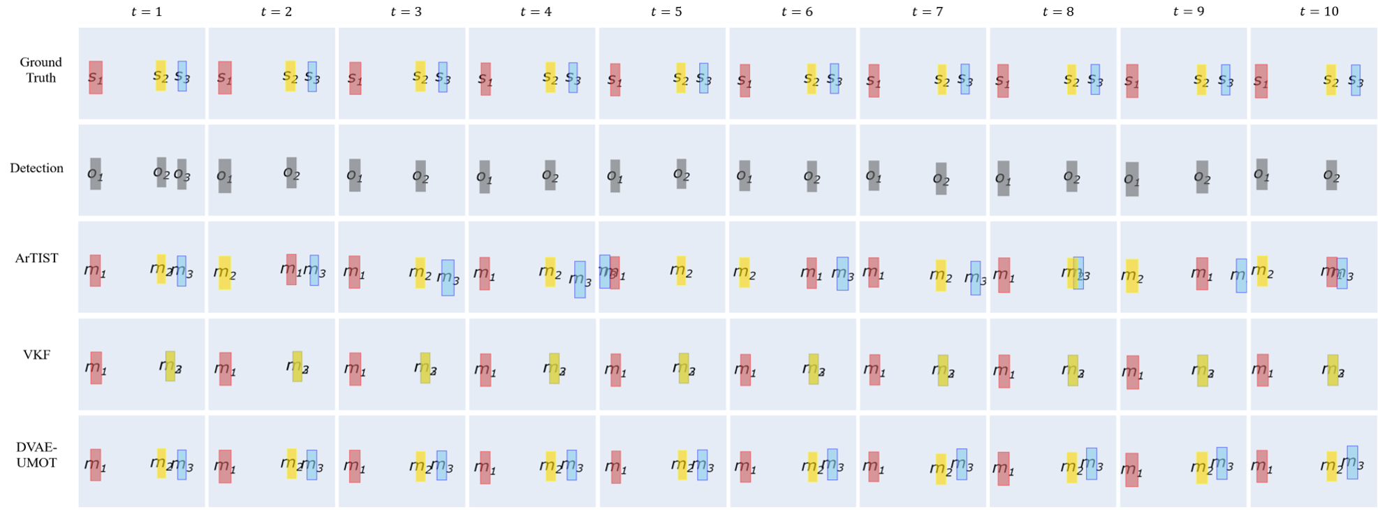
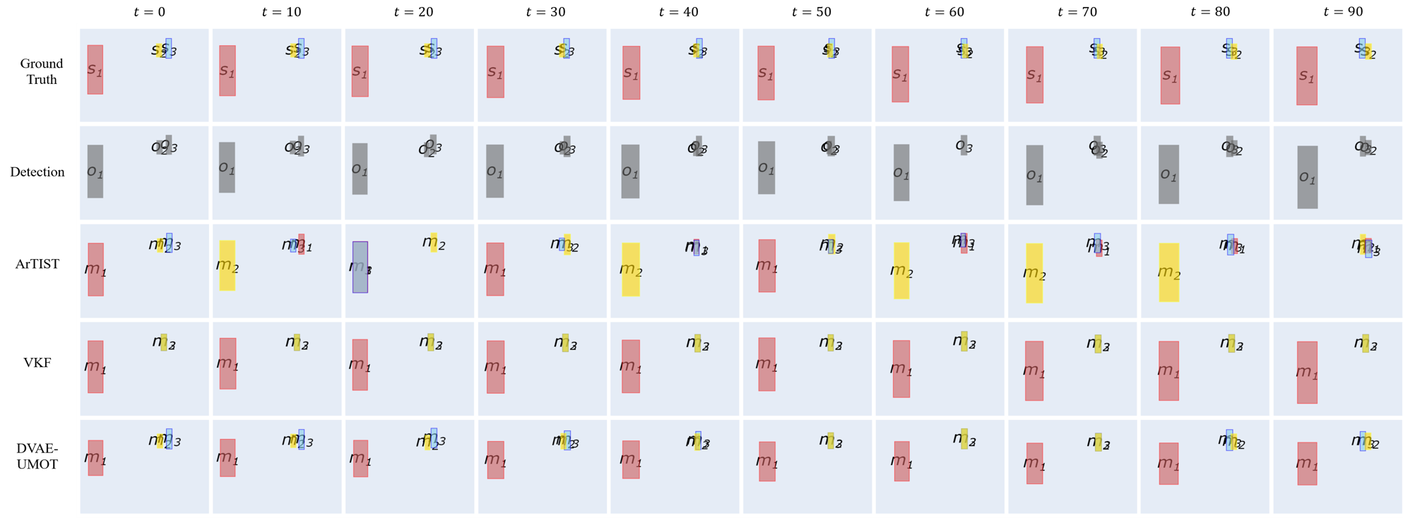
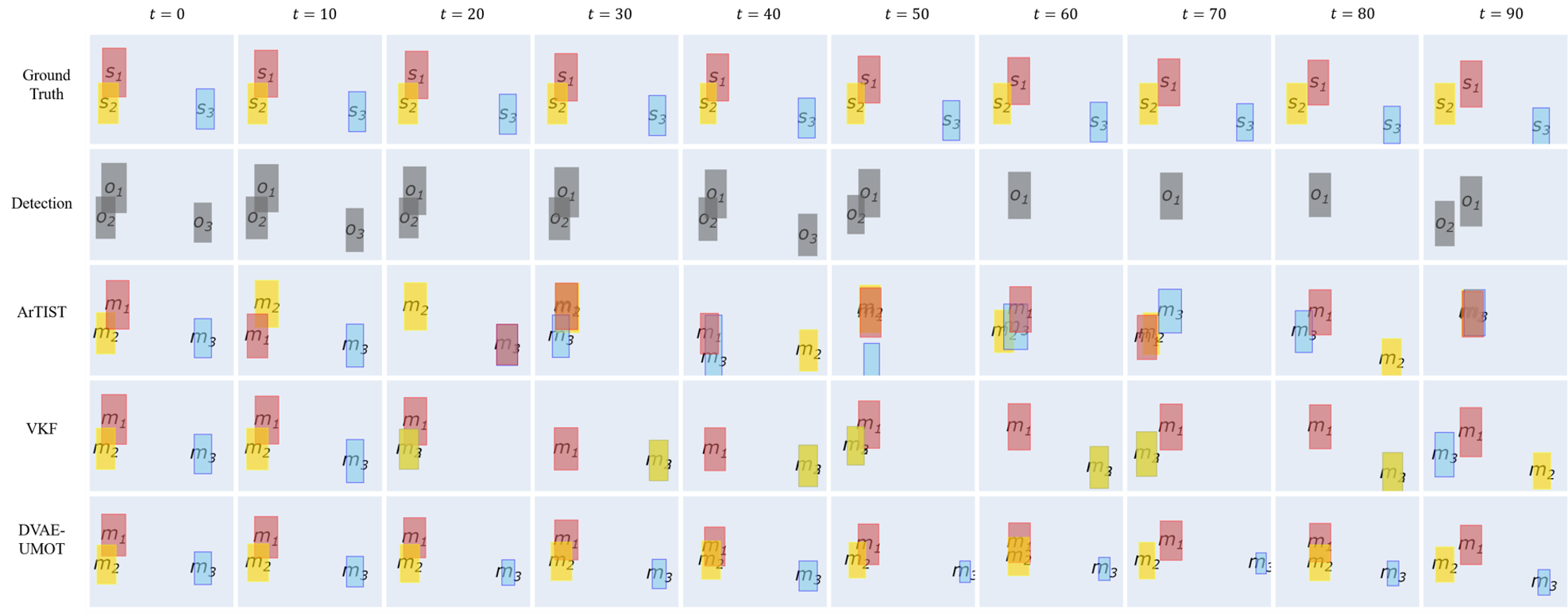
VI-D2 Examples of tracking results
To illustrate the behavior of each of the three models, we present three graphical examples of tracking results. In the first example plotted in Fig. 2 (top), the detection for Object 3 ( in the figure) is absent from and reappears after . But we limit the plot to for a better visualization. This is a case of long-term detection absence. An immediate identity switch occurs at for the ArTIST model. Then, the track obtained by ArTIST is no longer stable. We speculate the reason for the frequent identity switches made by ArTIST is that the estimated distributions do not correspond well to the true sequential position distributions, which is possibly due to the way these distributions are discretized. Besides the identity switches, the bounding boxes generated by ArTIST at , , and are not accurate. This causes a decrease of the tracking performance. For the VKF model, the estimated bounding boxes for Objects 2 and 3 ( and in the figure) overlap each other. This means that the two observations are both assigned to the same object, which is Object 2. From (33) and (34), we know that the value of the assignment variable depends on the posterior mean and variance vectors and , which themselves depend on the dynamical model. With a linear dynamical model, VKF is not able to correctly predict distinct and trajectories. Due to the very good dynamical modeling capacity of the DVAE, DVAE-UMOT still kept tracking despite of the long-term detection absence and generated reasonable bounding boxes for , which correspond well to the ground-truth bounding boxes of Object 3 ( in the figure).
The second example plotted in Fig. 2 (middle) illustrates the case where two persons cross each other. This is one of the most complicated situations that may cause an identity switch and even lead to tracking loss. Considering the limited space for the figure, we display the bounding boxes every ten frames to view the whole process of crossing. For , when the ground truth bouding boxes of Objects 2 and 3 ( and in the figure) strongly overlap, Detection disappears. Again, ArTIST exhibits frequent identity switches. Besides, at , the estimated bounding box is totally overlapped with that of . And at , the estimated bounding boxes for all of the three objects are getting very close to each other. This indicates that the identity switches can cause unreasonable trajectories estimation. For VKF, the observations for both Object 2 and 3 are assigned to the same target all along the sequence, due to and being close to each other, so that the estimated bounding boxes and overlap completely. In contrast, DVAE-UMOT displays a consistent tracking of the three objects. For , , and , the estimated bounding boxes and overlap due to the ground truth bounding boxes and strongly overlap each other. However, the tracking is correctly resumed at , with no identity switch (i.e., the crossing of Objects 2 and 3 is correctly captured by the model).
The third example displayed in Fig. 2 (bottom) is another more complicated situation with two objects very close to each other and frequent detection absence. At when observation disappears, both ArTIST and VKF lose one of the tracks, whereas DVAE-UMOT keeps a reasonable tracking of the three tracks. From to , both and are absent. The tracks inpainted by ArTIST are not consistent anymore and VKF still misses one track. However, even in this difficult scenario, DVAE-UMOT keeps on providing three reasonable trajectories.
VI-E Ablation study
VI-E1 Influence of
| MOTA | MOTP | IDF1 | IDs | IDs | MT | ML | FP | FP | FN | FN | |
|---|---|---|---|---|---|---|---|---|---|---|---|
| 0.01 | 35.9/32.8 | 84.5/84.8 | 66.6/65.5 | 4914/3216 | 1.6/1.0 | 2946/2714 | 916/913 | 96438/102062 | 31.3/33.1 | 96438/102062 | 31.3/33.1 |
| 0.02 | 65.5/61.8 | 84.2/84.7 | 81.3/79.8 | 5319/3073 | 1.7/1.0 | 3932/3652 | 407/379 | 50596/57291 | 16.4/18.6 | 50596/57291 | 16.4/18.6 |
| 0.03 | 74.9/70.0 | 83.1/84.3 | 86.1/84.4 | 5088/2853 | 1.7/0.9 | 4232/3931 | 158/160 | 36165/43777 | 11.7/14.2 | 36165/43777 | 11.7/14.2 |
| 0.04 | 79.1/75.1 | 81.3/83.5 | 88.4/86.7 | 4966/2862 | 1.6/0.9 | 4370/4067 | 50/64 | 29808/36990 | 9.7/11.9 | 29808/36990 | 9.7/11.9 |
| 0.05 | 76.4/75.6 | 79.2/82.6 | 87.1/87.1 | 4982/2919 | 1.6/0.9 | 4268/4066 | 42/53 | 33924/36088 | 11.0/11.7 | 33924/36088 | 11.0/11.7 |
| 0.06 | 69.2/70.1 | 76.9/82.0 | 83.5/84.4 | 5297/3005 | 1.7/1.0 | 3978/3845 | 73/137 | 44793/44598 | 14.5/14.5 | 44793/44598 | 14.5/14.5 |
| 0.07 | 59.8/66.8 | 74.8/80.3 | 78.9/82.9 | 5146/3000 | 1.7/1.0 | 3688/3775 | 188/285 | 59348/49646 | 19.2/16.1 | 59348/49646 | 19.2/16.1 |
| 0.08 | 48.5/60.6 | 73.1/79.4 | 73.3/79.9 | 5097/3119 | 1.7/1.0 | 3303/3637 | 337/432 | 76865/59220 | 24.9/19.2 | 76865/59220 | 24.9/19.2 |
We start our ablation study by analyzing the influence of . Table IV reports the MOT scores obtained with DVAE-UMOT as a function of . These experiments are conducted on the subset of short sequences. We report the results for both with and without fine-tuning SRNN in the E-Z step. Apart from the value of and the fine-tuning option, all other conditions are exactly the same across experiments.
Table IV shows that, whether fine-tuning SRNN in the E-Z step or not, the MOT scores first globally increase with ,66 6 Except for the MOTP score, which continually decreases with the increase of . This can be explained as follows. MOTP measures the precision of the position estimation for the matched bounding boxes. The estimated position in (29) is a weighted combination of the observation and the DVAE prediction. When increases, the contribution of the observation decreases and is closer to the DVAE prediction. Since the error of the DVAE prediction may accumulate over time, this finally decreases the position estimation accuracy. reach their optimal values for or (for most metrics), and then decrease for greater values. For confirmation, we have also computed the averaged empirical ratio of the detected bounding boxes (with the SDP detector), which is calculated as .77 7 Note that here denotes the position of the target matched with the observation at time frame . We omit the target positions that are not matched with any observation. This value equals to , and respectively for the short, medium and long sequence dataset. These values, which are close to each other because we used the same detector, correspond well to the value for the best performing model in Table IV. We can conclude that the model has better performance if the value of corresponds (empirically) to the detector performance.
Besides, we have also observed that the value of has an impact on the convergence of the DVAE-UMOT algorithm. Fig. 3 displays the MOTA score as a function of the number of DVAE-UMOT iterations (here with the fine-tuning of the DVAE model). It appears clearly that for too high values of , the model exhibits a lower and more hectic performance than for the optimal value.

VI-E2 Influence of fine-tuning
As mentioned in Section IV-E2, SRNN can either be fine-tuned or not in the DVAE-UMOT model. Table V shows the MOT scores obtained by DVAE-UMOT on the three test subsets with and without the fine-tuning of SRNN in the E-Z step.
| Dataset | Fine-tuning | MOTA | MOTP | IDF1 | IDs | IDs | MT | ML | FP | FP | FN | FN |
|---|---|---|---|---|---|---|---|---|---|---|---|---|
| Short | Fine-tune | 75.1 | 83.5 | 86.7 | 2862 | 0.9 | 4067 | 64 | 36990 | 11.9 | 36990 | 11.9 |
| No fine-tune | 79.1 | 81.3 | 88.4 | 4966 | 1.6 | 4370 | 50 | 29808 | 9.7 | 29808 | 9.7 | |
| Medium | Fine-tune | 73.1 | 84.0 | 85.9 | 3044 | 0.7 | 2705 | 136 | 54604 | 13.1 | 54604 | 13.1 |
| No fine-tune | 78.6 | 82.2 | 88.0 | 6107 | 1.5 | 2907 | 120 | 41747 | 9.9 | 41747 | 9.9 | |
| Long | Fine-tune | 65.6 | 84.9 | 81.6 | 8670 | 0.8 | 2286 | 67 | 171515 | 13.8 | 171515 | 13.8 |
| No fine-tune | 83.2 | 82.4 | 90.0 | 23081 | 2.3 | 2890 | 12 | 74550 | 7.3 | 74550 | 7.3 |
We observe that for all of the three datasets, not fine-tuning the DVAE model obtains the best overall performance (as measured by MOTA in particular). Though fine-tuning the DVAE model can indeed increase the MOTP score and decrease the number of identity switches, it does not improve the overall tracking performance. Indeed, fine-tuning increases the FP and FN numbers/proportions, and thus decreases the MOTA scores. Especially on the long sequence dataset, the MOTA score drops from to . The possible reason is that fine-tuning could make the model more sensible to detection noise, and lead to a generative model with worse performance.
VII Conclusion and Future Work
In this paper, we have proposed a deep LVGM and corresponding algorithm for MOT, called DVAE-UMOT. This method is based on VI at two levels. The first level is the pre-training of a DVAE model (in our experiments SRNN) on a synthetic single-object dataset; The DVAE is used within DVAE-UMOT as a deep probabilistic model of object dynamics. The second level is the estimation of the parameters of the overall DVAE-UMOT model, which is done on every test multi-object sequence to be processed. Observation-to-track association is done by estimating an assignment variable distribution while each object position distribution is estimated by combining the detection and the DVAE prediction. Our model is unsupervised, i.e., it does not use any manual annotation of ground-truth object position sequence for training, in fact it does not use any labeled dataset at all.
We evaluated the performance of the proposed algorithm by conducting experiments on a multi-object dataset derived from the MOT17 training set. Experimental results show that DVAE-UMOT obtains MOTA scores that are notably higher than those obtained by two state-of-the-art baselines. In particular, it largely reduces the identity switches compared to ArTIST and obtain consistently better results than VKF for almost all metrics. In case of detection absence and frequent occlusions, DVAE-UMOT can keep good tracking performance and generate reasonable bounding boxes to fill in the detection gaps. Compared to the linear motion model used in VKF (and in many other Kalman filter-based methods), the DVAE-based model is able to model more complex object dynamics and thus proves more accurate and robust for MOT in the VI framework. Finally, we conducted ablation studies to better understand the influence of several factors/settings on the DVAE-UMOT performance.
Of course, the quality of the visual information is essential to design a good MOT model. We demonstrated in this work that under the tracking-by-detection paradigm, modeling the motion information with a powerful non-linear DVAE model can lead to achieve quite good tracking performance. In the present study, we did not consider the object appearance information, and did not consider the track birth/death process as well, because we wanted the study to focus on the potential of the DVAE for modeling the object dynamics in a MOT framework. The design of a complete MOT system based on a DVAE should consider those two aspects, which is planned in our future works.
References
- [1] B.-n. Vo, M. Mallick, Y. Bar-Shalom, S. Coraluppi, R. Osborne, R. Mahler, and B.-t. Vo, “Multitarget tracking,” Wiley encyclopedia of electrical and electronics engineering, no. 2015, 2015.
- [2] W. Luo, J. Xing, A. Milan, X. Zhang, W. Liu, and T.-K. Kim, “Multiple object tracking: A literature review,” Artif. Intell., vol. 293, p. 103448, 2021.
- [3] M. Andriluka, S. Roth, and B. Schiele, “People-tracking-by-detection and people-detection-by-tracking,” in Proc. IEEE Int. Conf. Computer Vision Pattern Recogn. (CVPR), 2008, pp. 1–8.
- [4] N. Wojke, A. Bewley, and D. Paulus, “Simple online and realtime tracking with a deep association metric,” in Proc. IEEE Int. Conf. Image Process. (ICIP), 2017, pp. 3645–3649.
- [5] G. Ciaparrone, F. Luque Sánchez, S. Tabik, L. Troiano, R. Tagliaferri, and F. Herrera, “Deep learning in video multi-object tracking: A survey,” Neurocomputing, vol. 381, pp. 61–88, 2020.
- [6] S. Ren, K. He, R. Girshick, and J. Sun, “Faster R-CNN: Towards real-time object detection with region proposal networks,” in Advances in Neural Inform. Process. Systems (NeurIPS), vol. 28, 2015.
- [7] J. Redmon, S. Divvala, R. Girshick, and A. Farhadi, “You only look once: Unified, real-time object detection,” in Proc. IEEE Int. Conf. Computer Vision Pattern Recogn. (CVPR), 2016, pp. 779–788.
- [8] K. He, G. Gkioxari, P. Dollár, and R. Girshick, “Mask R-CNN,” in Proc. IEEE Int. Conf. Computer Vision (ICCV), 2017, pp. 2980–2988.
- [9] M. Babaee, Z. Li, and G. Rigoll, “Occlusion handling in tracking multiple people using RNN,” in Proc. IEEE Int. Conf. Image Process. (ICIP), 2018, pp. 2715–2719.
- [10] P. Bergmann, T. Meinhardt, and L. Leal-Taixe, “Tracking without bells and whistles,” in Proc. IEEE/CVF Int. Conf. Computer Vision (ICCV), 2019, pp. 941–951.
- [11] F. Saleh, S. Aliakbarian, H. Rezatofighi, M. Salzmann, and S. Gould, “Probabilistic tracklet scoring and inpainting for multiple object tracking,” in Proc. IEEE Int. Conf. Computer Vision Pattern Recogn. (CVPR), 2021, pp. 14 329–14 339.
- [12] A. Bewley, Z. Ge, L. Ott, F. Ramos, and B. Upcroft, “Simple online and realtime tracking,” Proc. IEEE Int. Conf. Image Process. (ICIP), pp. 3464–3468, 2016.
- [13] X. Zhou, V. Koltun, and P. Krähenbühl, “Tracking objects as points,” in Proc. Europ. Conf. Computer Vision (ECCV), 2020, pp. 474–490.
- [14] Y. Zhang, C. Wang, X. Wang, W. Zeng, and W. Liu, “FairMOT: On the fairness of detection and re-identification in multiple object tracking,” in Int. J. Comput. Vis., vol. 129, 2021, pp. 3069–3087.
- [15] A. Sadeghian, A. Alahi, and S. Savarese, “Tracking the untrackable: Learning to track multiple cues with long-term dependencies,” in Proc. IEEE Int. Conf. Computer Vision (ICCV), 2017, pp. 300–311.
- [16] A. Milan, S. H. Rezatofighi, A. Dick, I. Reid, and K. Schindler, “Online multi-target tracking using recurrent neural networks,” in Proc. AAAI Conf. Artif. Intell., 2017, p. 4225–4232.
- [17] J. Xiang, G. Zhang, and J. Hou, “Online multi-object tracking based on feature representation and Bayesian filtering within a deep learning architecture,” IEEE Access, vol. 7, pp. 27 923–27 935, 2019.
- [18] X. Wan, J. Wang, and S. Zhou, “An online and flexible multi-object tracking framework using long short-term memory,” in Proc. IEEE Int. Conf. Computer Vision Pattern Recogn. Workshops (CVPRW), 2018, pp. 1311–13 118.
- [19] B. Yang and R. Nevatia, “Multi-target tracking by online learning of non-linear motion patterns and robust appearance models,” in Proc. IEEE Int. Conf. Computer Vision Pattern Recogn. (CVPR), 2012, pp. 1918–1925.
- [20] Y. Liang and Y. Zhou, “LSTM multiple object tracker combining multiple cues,” in Proc. IEEE Int. Conf. Image Process. (ICIP), 2018, pp. 2351–2355.
- [21] C. Dicle, O. I. Camps, and M. Sznaier, “The way they move: Tracking multiple targets with similar appearance,” in Proc. IEEE Int. Conf. Computer Vision (ICCV), 2013, pp. 2304–2311.
- [22] L. Girin, S. Leglaive, X. Bie, J. Diard, T. Hueber, and X. Alameda-Pineda, “Dynamical variational autoencoders: A comprehensive review,” Found. Trends Mach. Learn., vol. 15, no. 1-2, pp. 1–175, 2021.
- [23] D. P. Kingma and M. Welling, “Auto-encoding variational Bayes,” in Proc. Int. Conf. Learn. Repres. (ICLR), 2014.
- [24] D. J. Rezende, S. Mohamed, and D. Wierstra, “Stochastic backpropagation and approximate inference in deep generative models,” in Proc. Int. Conf. Mach. Learn. (ICML), 2014, pp. 1278–1286.
- [25] P. Dendorfer, A. Ošep, A. Milan, K. Schindler, D. Cremers, I. Reid, S. Roth, and L. Leal-Taixé, “MOTChallenge: A benchmark for single-camera multiple target tracking,” Int. J. Comput. Vis., vol. 129, pp. 845–881, 2021.
- [26] Q. Chu, W. Ouyang, H. Li, X. Wang, B. Liu, and N. Yu, “Online multi-object tracking using CNN-based single object tracker with spatial-temporal attention mechanism,” in Proc. IEEE Int. Conf. Computer Vision (ICCV), 2017, pp. 4846–4855.
- [27] C. Kim, F. Li, A. Ciptadi, and J. M. Rehg, “Multiple hypothesis tracking revisited,” in Proc. IEEE Int. Conf. Computer Vision (ICCV), 2015, pp. 4696–4704.
- [28] T. Xiao, H. Li, W. Ouyang, and X. Wang, “Learning deep feature representations with domain guided dropout for person re-identification,” in Proc. IEEE Int. Conf. Computer Vision Pattern Recogn. (CVPR), 2016, pp. 1249–1258.
- [29] L. Leal-Taixé, C. Canton-Ferrer, and K. Schindler, “Learning by tracking: Siamese CNN for robust target association,” Proc. IEEE Int. Conf. Computer Vision Pattern Recogn. Workshops (CVPRW), pp. 418–425, 2016.
- [30] J. Son, M. Baek, M. Cho, and B. Han, “Multi-object tracking with quadruplet convolutional neural networks,” in Proc. IEEE Int. Conf. Computer Vision Pattern Recogn. (CVPR), 2017, pp. 3786–3795.
- [31] Y. Ban, X. Alameda-Pineda, L. Girin, and R. Horaud, “Variational Bayesian inference for audio-visual tracking of multiple speakers,” IEEE Trans. Pattern Anal. Mach. Intell., vol. 43, no. 5, pp. 1761–1776, 2021.
- [32] K. Fang, Y. Xiang, X. Li, and S. Savarese, “Recurrent autoregressive networks for online multi-object tracking,” in IEEE Winter Conf. Appl. Comput. Vis. (WACV), 2018, pp. 466–475.
- [33] J. Luiten, I. E. Zulfikar, and B. Leibe, “Unovost: Unsupervised offline video object segmentation and tracking,” in IEEE Winter Conf. Appl. Comput. Vis. (WACV), 2020, pp. 1989–1998.
- [34] S. Karthik, A. Prabhu, and V. Gandhi, “Simple unsupervised multi-object tracking,” 2020.
- [35] Z. He, J. Li, D. Liu, H. He, and D. Barber, “Tracking by animation: Unsupervised learning of multi-object attentive trackers,” in Proc. IEEE Int. Conf. Computer Vision Pattern Recogn. (CVPR), 2019, pp. 1318–1327.
- [36] E. Crawford and J. Pineau, “Exploiting spatial invariance for scalable unsupervised object tracking,” Proc. AAAI Conf. Artif. Intell., vol. 34, no. 04, pp. 3684–3692, 2020.
- [37] Y. Pu, Z. Gan, R. Henao, X. Yuan, C. Li, A. Stevens, and L. Carin, “Variational autoencoder for deep learning of images, labels and captions,” in Advances in Neural Inform. Process. Systems (NeurIPS), 2016, p. 2360–2368.
- [38] X. Li and J. She, “Collaborative variational autoencoder for recommender systems,” in Proc. ACM SIGKDD Int. Conf. Knowl. Discov. Data Min., 2017, p. 305–314.
- [39] L. Maaløe, C. K. Sønderby, S. K. Sønderby, and O. Winther, “Auxiliary deep generative models,” in Proc. Int. Conf. Mach. Learn. (ICML), vol. 48, 2016, pp. 1445–1453.
- [40] L. Yingzhen and S. Mandt, “Disentangled sequential autoencoder,” in Proc. Int. Conf. Mach. Learn. (ICML), vol. 80, 2018, pp. 5670–5679.
- [41] S. Leglaive, X. Alameda-Pineda, L. Girin, and R. Horaud, “A recurrent variational autoencoder for speech enhancement,” in Proc. IEEE Int. Conf. Acoust., Speech, Signal Process. (ICASSP), 2020, pp. 371–375.
- [42] M. J. Wainwright and M. I. Jordan, “Graphical models, exponential families, and variational inference,” Found. Trends Mach. Learn., vol. 1, no. 1–2, p. 1–305, 2008.
- [43] C. M. Bishop, Pattern Recognition and Machine Learning. Berlin: Springer-Verlag, 2006.
- [44] G. Parisi and R. Shankar, “Statistical field theory,” Phys. Today, vol. 41, no. 12, p. 110, 1988.
- [45] M. D. Hoffman, D. M. Blei, C. Wang, and J. Paisley, “Stochastic variational inference,” J. Mach. Learn. Res., vol. 14, no. 4, pp. 1303–1347, 2013.
- [46] D. Geiger, T. Verma, and J. Pearl, “Identifying independence in Bayesian networks,” Networks, vol. 20, no. 5, pp. 507–534, 1990.
- [47] M. Fraccaro, S. K. Sønderby, U. Paquet, and O. Winther, “Sequential neural models with stochastic layers,” in Advances in Neural Inform. Process. Systems (NeurIPS), 2016, p. 2207–2215.
- [48] R. J. Williams and D. Zipser, “A learning algorithm for continually running fully recurrent neural networks,” Neural Comp., vol. 1, no. 2, pp. 270–280, 1989.
- [49] P. F. Felzenszwalb, R. B. Girshick, D. McAllester, and D. Ramanan, “Object detection with discriminatively trained part-based models,” IEEE Trans. Pattern Anal. Mach. Intell., vol. 32, no. 9, pp. 1627–1645, 2010.
- [50] F. Yang, W. Choi, and Y. Lin, “Exploit all the layers: Fast and accurate CNN object detector with scale dependent pooling and cascaded rejection classifiers,” in Proc. IEEE Int. Conf. Computer Vision Pattern Recogn. (CVPR), 2016, pp. 2129–2137.
- [51] H. W. Kuhn, “The Hungarian method for the assignment problem,” Nav. Res. Logist. Q., vol. 2, no. 1-2, pp. 83–97, 1955.
- [52] S. Manen, M. Gygli, D. Dai, and L. Van Gool, “Pathtrack: Fast trajectory annotation with path supervision,” in Proc. IEEE Int. Conf. Computer Vision (ICCV), 2017, pp. 290–299.
- [53] K. Bernardin and R. Stiefelhagen, “Evaluating multiple object tracking performance: The CLEAR MOT metrics,” EURASIP J. Image Video Process., vol. 2008, 2008.
- [54] E. Ristani, F. Solera, R. Zou, R. Cucchiara, and C. Tomasi, “Performance measures and a data set for multi-target, multi-camera tracking,” in Proc. Europ. Conf. Computer Vision (ECCV). Springer, 2016, pp. 17–35.
Supplementary material of
Unsupervised multiple-object tracking
with a dynamical variational autoencoder
Xiaoyu Lin, Laurent Girin, Xavier Alameda-Pineda, IEEE Senior Member
Appendix A DVAE-UMOT algorithm calculation details
A-A E-S Step
Here we detail the calculation of the posterior distribution . Using (11), the first expectation term in (23) can be developed as:
Since for any pair , the assignment variable follows a discrete posterior distribution, we can denote its values by
which will be calculated later in the E-W Step. With this notation, we have:
The second expectation in (23) cannot be computed analytically as a distribution on because of the non-linearity in the decoder and in the encoder. In order to avoid a tedious sampling procedure and obtain a computationally efficient solution, we further approximate this term by assuming , where is the mean value of the posterior distribution of estimated at the previous iteration. By using this approximation, the term is now considered as a constant.
In addition, we observe that the second term of (23) can be rewritten as:
since both the DVAE joint distribution and posterior distribution factorise over the objects, as formalized in (15) and (17). As a consequence, the posterior distribution of factorises over the tracked object:
and therefore:
| (41) |
In the above equation, the expectation term cannot be calculated in closed form. As usually done in the DVAE methodology, it is thus replaced by a Monte Carlo estimate using sampled sequences drawn from the DVAE inference model. Let us denote by such a sampled sequence. In the present work, we use single point estimate, thus obtaining:
We observe that the -th element of the previous factorisation is a distribution over conditioned by . As for , the dependency with is non-linear and therefore would impede to obtain a computationally efficient closed-form solution. In the same attempt of avoiding costly sampling strategies, we approximate the previous expression replacing with , obtaining:
with
since the term becomes a constant.
Another interesting consequence of sampling is that the dependency with the future observations of disappears. Indeed, since we are sampling at every time step, the future posterior distributions do not depend on , and therefore the posterior distribution of will not depend on the future observations.
The two distributions in the above equation are Gaussian distributions defined in (5), and (12). Therefore, it can be shown that the variational posterior distribution of is a Gaussian distribution: with covariance matrix and mean vector provided in (28) and (29) respectively, and recalled here for completeness:
where and are simplified notations for and respectively, denoting the variance and mean vector estimated by the DVAE for object at time frame .
A-B E-Z Step
A-C E-W Step
Here we detail the calculation of the posterior distribution . Applying the optimal update equation (2) to , we have:
Using (10), we derive:
Using (11), the expectation term can be developed as:88 8 In fact, the posterior distribution is also conditioned on and . We use this abuse of notation for concision.
Combining (13) and the previous result, we have:
which we can rewrite
with
The assignment variable follows a discrete distribution and we denote:
Using the fact that both and are multivariate Gaussian distributions (defined in (12) and (27)–(29), respectively), the previous expectation can be calculated in closed form:
By using (14), the previous result, and normalizing to 1, we finally get:
where
A-D M Step
Here we detail the calculation of . In the ELBO expression (19), only the first term depends on :
By computing the derivative of with respect to and setting it to 0, we find the optimal value of that maximizes the ELBO:
Appendix B Cascade initialization of the position vector sequence
For the initialization of the position vector, we first split the long sequence indexed by into smaller sub-sequences indexed by . For the first sub-sequence, the mean vector sequence is initialized as the detected vector at the first frame repeated for times with a arbitrary order of assignment. Thus, there are as many tracked sources as initial detections, i.e., this implicitly sets . The subsequence of object position vectors is initialized with the same values as for the mean vector. Then, we run the DVAE-UMOT algorithm on the first subsequence for iterations. Next, we initialize the mean vector sequence of the second subsequence with repeated for times (and the same for ). And so on for the following subsequences. Finally, the initialized subsequences are concatenated together to form the initialized whole sequence. The pseudo-code of the cascade initialization can be found in Algorithm 2.
| ); |
| ; |
| ; |
Appendix C SRNN implementation details
In our MOT set-up, both and are of dimension 4. The SRNN generative distributions in the right-hand side of (37) are implemented as:
where the function in (C) is implemented by a forward RNN and denotes the RNN hidden state vector, the dimension of which is set to 8. In practice, LSTM networks are used. The function in (C) is implemented by a dense layer of dimension 16, with the tanh activation function, followed by a linear layer, which outputs are the parameters . The function in (C) is implemented by two dense layers of dimension 8, 8 respectively, with the tanh activation function, followed by a linear layer, which outputs are the parameters .

Appendix D Synthetic trajectory dataset generation
We generate the trajectory of each coordinate of the bounding box, namely , , and , to from the bounding box sequence. While the trajectory of one coordinate is generated using piece-wise combinations of elementary dynamic functions, which are: static , constant velocity , constant acceleration and sinusoidal (allowing for circular trajectories) . That’s to say, we split the whole sequence into several segments, and each segment is dominated by a certain elementary dynamic function.
The number of segments is first uniformly sampled in the set . We then sample segment lengths that sum up to . This defines the segment boundaries . For each segment, one of the four elementary functions is randomly selected. The function parameters are sampled as follow: , , and . The two remaining parameters, and , are set to the values needed to ensure continuous trajectories, thus initialising the trajectories at every segment, except for the first one. The very initial trajectory point is sampled randomly from . And the initial width is sampled from a log-normal distribution . Finally, the ratio between the height and width is supposed to be constant with respect to time. It is sampled from a log-normal distribution and the height is obtained by multiplying the width and the ratio. More implementation details can be found in Algorithm 3.
| Sample trajectory function parameters using ; |
In our experiments, the total sequence length of the generated trajectories equals to frames. And the maximum number of segments is set to . The parameters of the , , , , , and distributions are determined by estimating the statistical characteristics of publicly published detections of the MOT17 training dataset. More precisely, we estimated the empirical mean and standard deviation of the speed and acceleration for all matched detection sequences (i.e., the first and second order differentiation of the position sequences).