Quasiparticle density of states and triplet correlations in superconductor/ferromagnetic-insulator structures across a sharp domain wall
Abstract
A ferromagnetic insulator (FI) in contact with a superconductor (S) is known to induce a spin splitting of the BCS density of states at the FI/S interface. This spin splitting causes the Cooper pairs to reduce their singlet-state correlations and acquire odd-in-frequency triplet correlations. We consider a diffusive FI/S bilayer with a sharp magnetic domain wall in the FI and study the local quasiparticle density of states and triplet superconducting correlations. In the case of collinear alignment of the domains, we obtain analytical results by solving the Usadel equation. For a small enough exchange field or weak superconductivity, we also find an analytical expressions for arbitrary magnetic textures, which reveals how the triplet component vector depends on the local magnetization of the FI. For an arbitrary angle between the magnetizations and the strength of the exchange field, we numerically solve the problem of a sharp domain wall. We finally propose two different setups based on FI/S/F stacks, where F is a ferromagnetic layer, to filter out singlet pairs and detect the presence of triplet correlations via tunneling differential conductance measurements.
I Introduction
The exchange coupling at the interface between a ferromagnetic insulator (FI) and a thin superconducting layer (S) can lead to a spin-splitting of the density of states (DoS) in the S layer, as observed in numerous experiments Moodera et al. 1988; Hao et al. 1990; Meservey and Tedrow 1994; Strambini et al. 2017; Hijano et al. 2021. Recently there has been a renewed interest in these systems due to various proposed applications. These applications include spin valves Miao et al. 2014; De Simoni et al. 2018, spin batteries Jeon et al. 2020; Ojajärvi et al. 2021, magnetometers Alidoust et al. 2013; Strambini et al. 2015, thermometers Giazotto et al. 2006; Giazotto et al. 2015a, caloritronic devices Giazotto and Bergeret 2013; Giazotto et al. 2015b; Giazotto and Bergeret 2020, thermoelectric elements Machon et al. 2013; Ozaeta et al. 2014, and radiation detectors Heikkilä et al. 2018; Geng et al. 2020. FI/S structures have also been explored in the context of Majorana fermions in semiconducting wires Oreg et al. 2010; Lutchyn et al. 2010; Dai et al. 2021.
Most of these applications require a robust superconducting gap with a sizable spin-splitting. This can be achieved, for example, in EuS/Al systems, Hao et al. 1990; Moodera et al. 2007; Strambini et al. 2017; De Simoni et al. 2018; Hijano et al. 2021, where the interfacial exchange interaction leads to a sharp spin-splitting in S layers with thicknesses smaller than the coherent length. On the theoretical side, the effect of the interfacial exchange field and the induced spin-splitting on the superconducting state has been studied in numerous works Tokuyasu et al. 1988; Virtanen et al. 2020; Rouco et al. 2019; Hijano et al. 2021. Most of these works assume a homogeneous spin-splitting field. This assumption is justified, even in a multidomain situation, if the characteristic domain size of EuS is much longer than the superconducting coherence length .
There are, however, situations in which the domain size may be of the order of the superconducting coherence length. The effect of domain walls in magnetic and insulating ferromagnets on adjacent superconductors has been studied theoretically Aladyshkin et al. 2003; Houzet and Buzdin 2006; Bobkova and Bobkov 2019; Rabinovich et al. 2019; Aikebaier et al. 2019 and experimentally Yang et al. 2004; Strambini et al. 2017, while Ref. Linder and Halterman 2014 studied the influence of domain-wall dynamics on superconductivity. In particular, Ref. Strambini et al. 2017 provided experimental evidence that EuS consists of multiple domains with a size of the order of the coherence length of the Al layer attached to it. The authors of that work contrast spectroscopic measurements with a theoretical model that assumed alternating up/down domains of different sizes. In the present work, we generalize this approach and study a FI/S structure with two non-collinear magnetic domains.
Despite the amount of experimental work on FI/S systems, almost all of it focuses on studying its quasiparticle spectrum. There is, however, an interesting aspect that is not often mentioned in these works. The mere existence of an interfacial exchange field leads to conversion of singlet superconducting correlations to triplet ones Bergeret et al. 2005; Cottet 2011; Bergeret et al. 2018; Heikkilä et al. 2019. The induced triplet component has a total zero spin projection if the FI consists of a single domain with homogeneous magnetization. However, in FI/S systems with non-collinear magnetization, triplet components with different spin-projections may coexist with the singlet one.
In this work, we study the equilibrium properties of a FI/S bilayer with a sharp domain wall separating two magnetic domains. We present an analytical solution for the Usadel equation for a FI/S bilayer consisting of two semi-infinite magnetic domains with collinear magnetization and non-collinear magnetization in the weak exchange field limit; and use numerical methods to solve the non-collinear case with arbitrary exchange field strength. Additionally, we study the spatial evolution of the triplet correlations near a domain wall and propose a method to detect them using tunneling spectroscopy of an additional ferromagnetic layer. The work is organized as follows: In Sec. II we present the main equations describing a diffusive superconductor attached to a FI layer with multiple domains and a general Lagrangian from which one can derive the Usadel equation. We identify conserved quantities within each domain. In Sec. III we use these integrals of motion to derive an analytical expression for the DoS of a FI/S system with two collinear domains of arbitrary magnitude. In Sec. IV we generalized these results to the case of non-colinear magnetization. Finally, in Sec. V we study the properties and spatial evolution of the triplet correlations, and suggest a way to detect them. We summarize the results in Sec. VI.
II The Model
We consider a FI/S bilayer structure, see Fig. 1. A diffusive superconducting film is placed on top of a FI film. A typical example is Eu/Al studied in several papers Hao et al. 1990; Moodera et al. 2007; Strambini et al. 2017; De Simoni et al. 2018; Hijano et al. 2021. In these systems, the EuS film is polycrystalline and magnetic domains with sharp boundaries are very common, in particular before the first magnetization of the EuS Strambini et al. 2017.
To describe the system we use the quasiclassical Green’s function (GF) formalism extended to treat spin-dependent fields Bergeret et al. 2005. In this case the GF is a matrix in Nambu-spin space. In the diffusive limit, it does not depend on momentum and is determined by the Usadel equation Usadel 1970. The interfacial exchange field is introduced as an effective boundary condition at the FI/S interface Bergeret et al. 2012; Eschrig et al. 2015; Heikkilä et al. 2019. Assuming that the thickness of the S layer is smaller than the coherence length one can integrate the Usadel equation over the thickness to reduce the dimension of the problem. The resulting Usadel equation for the retarded GF reads
| (1) |
where , is the diffusion constant, is the energy, is the effective exchange field stemming from the interface and is the order parameter. The exchange field is only finite at the FI/S interface, and we approximate it as , where is the exchange field at the interface, and is the thickness of an effective layer over which the exchange interaction is finite Heikkilä et al. 2019; Zhang et al. 2019. After integration over the direction the effective exchange field is given by Hijano et al. 2021. It is worth noting that the critical temperature of the S layer decreases with decreasing thickness, such that at low temperatures superconductivity can be fully suppressed when Chandrasekhar 1962; Clogston 1962. In this work we consider values of the exchange field which are weak enough such that superconducting ordering and the exchange field coexist. The matrices (), in Eq. 1 are the Pauli matrices in the spin (Nambu) space. The general structure of is:
| (2) |
where and are the normal and anomalous GF in spin-space.
The GF satisfies the normalization condition , and can be parametrized with the help of the generalized -parametrization Ivanov and Fominov 2006
| (3) |
which is described by two scalars and and the vector . and satisfy the condition
| (4) |
and describe the singlet and triplet correlations respectively. If is homogeneous then is parallel to it, but in general, as we show on Sec. V, is not parallel to the local exchange field.
In the above parametrization, the Usadel equation reduces to following set of equations
| (5a) | ||||
| (5b) | ||||
It is useful for finding analytical solutions to write a Lagrangian which leads to Equations (5) as the Euler-Lagrange equations:
| (6) |
with . This Lagrangian coincides with the form of the non-linear -model from which the Usadel equation can also be derived Kamenev 2011; Altland and Simons 2010.


The above equations are valid for arbitrary magnetic textures. On the following, we focus on the situation of two semi-infinite magnetic domains with constant magnetization. The domains are separated by a sharp domain wall at with a length much smaller than the superconducting coherence length. We assume that one of the domains () is polarized along the axis, whereas the magnetization of the other domain () forms an angle with the axis, see Fig. 1. At distances much larger than the coherence length the GF takes its bulk form . The system has translational symmetry along the and directions, so the parameters only depend on the coordinate.
On each domain the Lagrangian (6) does not depend explicitly on the position , so the corresponding Hamiltonian is an integral of motion in each domain. The conserved quantity is namely given by
| (7) |
The values of far away from the domain wall, where the GF is given by the bulk solution and therefore constant in space can be easily obtained:
| (8) |
where the bulk values and of the GF are given by the inverse relations of Eq. (2)
| (9a) | ||||
| (9b) | ||||
| (9c) | ||||
and the bulk GF is given by
| (10a) | ||||
| (10b) | ||||
with , . In the following section we use this expressions to define integrals of motion that allow for an analytical solution when the magnetic domains are collinear.
III Domains with collinear magnetization

If the magnetization of the two domains are collinear, the problem can be greatly simplified. Firstly, only the component of the vector parallel to the magnetization is non-zero. Without any loss of generality we assume that the magnetizations lie in the axis, such that . In this case, Eq. (5) reads:
| (11a) | ||||
| (11b) | ||||
where . One can combine these equations to obtain two decoupled equations for each spin component:
| (12) |
where respectively describe the spin up and down components of the GF.
Since the problem is decoupled in spin space, one can derive equations in (12) from two independent Lagrangians:
| (13) |
Because do not depend explicitly on , the following quantities are conserved in space:
| (14) |
These expressions can be evaluated at the bulk where the spatial derivative vanishes and the GF is given by the bulk solution [see Eq. (10)]. and are given by the spin components and respectively, where the sign corresponds to the up/down spin index
| (15) |
Here are the value of at the bulk. In the following we omit the spin subscript to simplify the notation. Substituting equation (14) into (15) and applying trigonometric identities, we arrive at
| (16) |
Equation (16) does not explicitly contain the independent variable . Taking the square root on both sides of the equation we obtain a first order differential equation which can be integrated to obtain
| (17) |
where is chosen such that , and that the exponential functions decay away from the domain wall. is the value of the exchange field in the left () and right () domains.
From Eq. (17) one can obtain the spatial dependence of by determining the constants . For this we use the fact that the GF and its derivative are continuous at the domain wall. Applying this condition, we obtain the values of the constants in Eq. (17)
| (18) |
where , and the upper and lower signs correspond to the left and right domains respectively. The sign of the square root on Eq. (18) is chosen such that the DoS is positive and the solution is physically meaningful. Setting the order parameter to zero in the right domain and the exchange fields to zero, we recover the results by Altland et al. Altland et al. 2000 for a singlet S/N junction. Golubov et al. Golubov et al. 2005 also followed a similar procedure to study the DoS at ferromagnetic and normal layers on S(FN) and S(FF) structures.
Equation (17) together with Eq. (18) determines the analytical solution for the two semi-infinite collinear domains. The local DoS is related to the GF through the expression
| (19) | ||||
As first example, we assume that the magnetizations of the two domains are opposite in direction but equal in amplitude (). In this case the DoS at the domain wall () has a simple form
| (20) |
which leads to the red curves in Fig. 2. This analytical result coincides with the numerical result obtained in Refs. Strambini et al. 2017 and Aikebaier et al. 2019 for a narrow domain wall between two collinear domains. In Fig. 2 we show the spatial dependence of the DoS for spin-up electrons in the antiparallel magnetization configuration. Far form the domain wall the coherent peaks of the DoS are well defined (dashed lines). The presence of the domain wall smears the peak. In Fig. 3(a) we show the spatial dependence of the full DoS. Specifically, Fig. 3 (b) shows the DoS at the values of indicated by the colored lines in panel (a). The magnitude of the exchange field is the same on both domains so the total DoS is symmetric with respect to . For large enough distances away from the domain wall the BCS peak is shifted by the exchange field to . Near the domain wall, there is a crossover between the position of the spin up/down peaks over a length scale of the order of the superconducting coherence length . Notice that around the domain wall, the inner peak is broader and lower than the outer peak [see Fig. 3(b)], but the gap edge remains, as expected, at .
A second interesting example is when the exchange field is only finite in one of the regions (). This corresponds to a S layer only partly covered by the the FI layer. In Fig. 3(c) we show the local DoS in this case. The spin-split DoS at evolves into the usual BCS DoS at , over the length around the domain wall. The splitting of the DoS peaks does not decrease smoothly as one would expect in a system where the exchange field is suppressed gradually over a length much larger than . Namely, the inner peak is smeared in a similar way to the anti-parallel magnetization case [Fig. 3(b)], such that the DoS has the same “shark-fin” shape right at [red curve on Fig. 3(d)]. All above predictions could be proven by performing local tunneling spectroscopy measurements.
IV Non-collinear magnetization
In the previous section we focused on the collinear magnetization case in which it was possible to decouple the components of the Usadel equation. In that case, we can find conserved quantities, Eq. (15), and obtain analytically expressions for the GF. If the magnetizations are non-collinear the system lacks enough symmetries to reduce the number of coupled equations. Nonetheless, it is possible to solve the Usadel equation (5) analytically in the weak superconducting or weak exchange field limits, as discussed in the next subsections. Later below, we study the two domain situation for an arbitrarily large exchange field numerically 11 1 Domain walls with non-collinear magnetization may induce stray fields that could affect superconductivity. In this work, we neglect the orbital effects of stray fields and assume that the superconducting gap is homogeneous in the S layer. The stray fields depend on the geometry and size of the magnetic layer, so we assume that the FI geometry is such that it minimizes the magnetostatic energy and, therefore, the stray fields. For any angle , the stray field can be minimized if the orientation of the domains is chosen to be with respect to the axis..
IV.1 Weak superconductivity
If the superconductor is close to the critical temperature , the Usadel equation (5) can be linearized for small order parameter (). This limit is very illustrative to understand the length scales involved in the system.
Near the GF can be approximated by . The linearized Usadel equation determines the anomalous GF
| (21a) | ||||
| (21b) | ||||
where the spin structure is
| (22) |
where is the singlet and , the triplet components. For the two semi-infinite domain structure considered in this work, the solution to Eq. (21) is given by
| (23a) | ||||
| (23b) | ||||
where and are the asymptotic values at of the singlet and triplet components respectively, and , . The triplet can be written as the sum of the component parallel to the local exchange field, second term in Eq. (23b), and the component orthogonal to it proportional to the vector , with . The component perpendicular to the local exchange field decays away from the domain wall over the length , whereas the correction to the bulk (parallel) solution is significant at distances less than .
IV.2 Weak exchange field
Another analytical limiting case is the case of a weak exchange field (). In this case one can linearize the Usadel equation (5) and solve the system for an arbitrary magnetization texture. In zeroth order in , only the singlet component of the GF is finite and it is given by Eqs. (9-10) setting
| (24a) | |||
| (24b) | |||
To first order in , both and are not corrected. Whereas the triplet vector is determined by
| (25) |
where () is the energy dependent coherence length. The solution of this equation can be written as
| (26) |
where is the Green’s function of the differential equation (25) determined by
| (27) |
Solving Eq. (27), we arrive at
| (28) |
This result shows explicitly the spatial dependence of the triplet vector. It is determined by the exchange field averaged over the length . For example if the spatial variation of the exchange field is slower than the length then the vector is locally parallel to the exchange field. In particular, in the case of two magnetic domains separated by a smooth (respect to the length ) domain wall, the vector is always aligned with the local field .
In this work we are mainly interested in sharp domain walls , i.e. domain-walls with sizes much smaller than . If we model such situation by a step-like exchange field with , then the triplet vector at the left and right side of the domain wall can be obtained from Eq. (28):
| (29) |
As expected, at distances much larger than from the domain wall is parallel to the local exchange field. In contrast, the transverse component to the field is maximized at the domain wall and decays over away from it. The above analytical results are obtained for weak exchange fields. In the next section we consider arbitrarily strong exchange field.
IV.3 Arbitrary exchange field
In this section we consider two domains with an arbitrarily large exchange field and arbitrary angle between the domains magnetization and solve numerically the Usadel equation. For this it is convenient to differentiate twice Eq. (4) and substitute the result into Eq. (5). We thus arrive at Baker et al. 2016; Aikebaier et al. 2019
| (30a) | ||||
| (30b) | ||||
| (30c) | ||||
We solve the above equations numerically for a S layer of finite length . The domain wall is located at . The spectral current vanishes at the boundaries with vacuum. In the generalized -parametrization this translates into the following boundary conditions for Eq. (30)
| (31a) | ||||
| (31b) | ||||
| (31c) | ||||
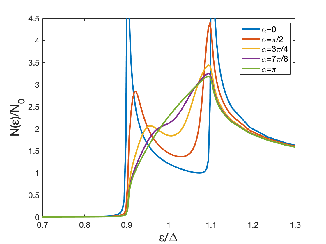
In Fig. 4 we show the computed total DoS at the domain wall for domains with the same exchange field magnitude and different orientations [see Fig. 1]. In the case, the exchange field is uniform along the sample, so the DoS is the homogeneous spin-split BCS. Both peaks are broadened and lowered by increasing , and the DoS exhibits the “shark-fin” when the magnetizations are anti-parallel. The spin-splitting is still visible up to values of .
V Triplet pair correlations in FI/S structures and their detection
In the previous sections, we have analyzed the quasiparticle spectrum. Here we focus on another aspect of the FI/S structures: the superconducting triplet pair-correlations. These appear due to the finite interfacial exchange field that converts conventional singlet into triplet pairs Bergeret et al. 2001; Bergeret et al. 2005.
Within our model, pair correlations are described by the anomalous component introduced in Eq. (2), which in the spin-space has the general structure given by Eq. (22). Because we consider the strict diffusive limit, all components of are isotropic in momentum (s-wave symmetry). From the Fermi statistics for Fermion pairs it follows that is an even function of frequency whereas are odd Berezinskii 1974; Bergeret et al. 2005; Tanaka et al. 2012; Linder and Balatsky 2019. The following association between the different components of the condensate and the spin state of electron pairs can be made Eschrig 2011
| (32) | ||||
| (33) | ||||
| (34) | ||||
| (35) |
In other words, each triplet component of the condensate is associated with maximally entangled states. In a conventional BCS superconductor, only the singlet component is finite. Triplet components are finite in the presence of an exchange field. In a homogeneous case, we choose the spin quantization axis along the magnetization direction, e.g., the axis. The only finite components of the condensates are, in this case, and . All triplet components may appear in a multidomain situation with arbitrary magnetization directions.

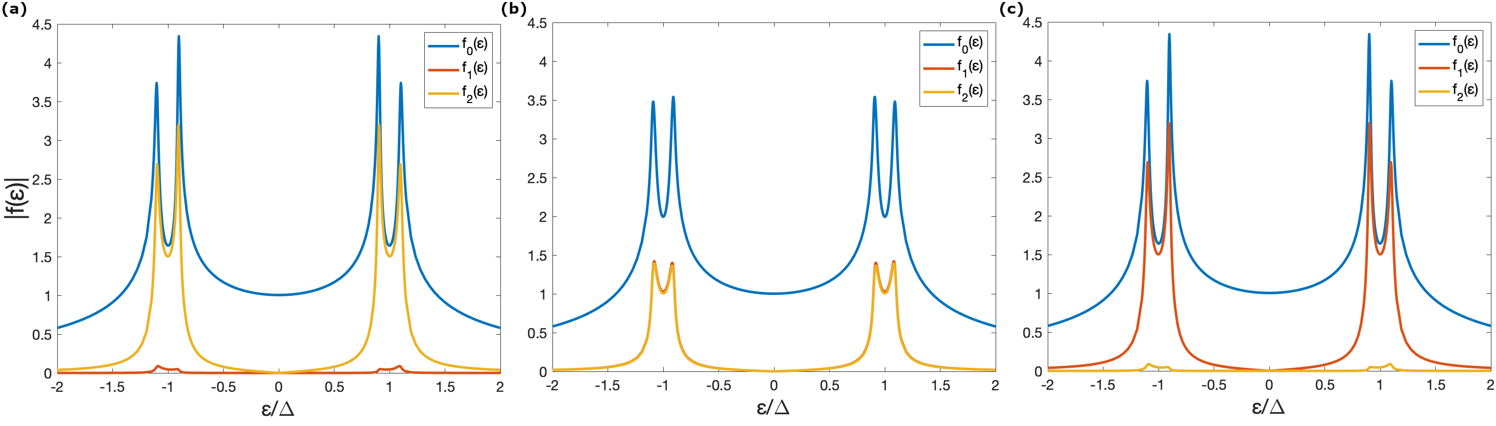
Here we study the singlet and triplet correlations in a FI/S bilayer with two non-collinear domains, see Fig. 1. We assume that such that two components , are finite. The length of S is . In Fig. 5 we show the spatial dependence of the singlet and triplet components of for all energies, calculated numerically. All condensate components show peaks at and decay to zero at energies much larger than the gap. Inside the gap the amplitude of the singlet is of the order of 1. In contrast, at the triplet components are of the order of , where is the Dynes parameter Dynes et al. 1978 describing inelastic scattering. They increase linearly at small energies and become comparable to the singlet component within the range . Far away from the domain wall, only the triplet component parallel to the local exchange field is finite. Both components, and , have the same magnitude at the domain wall, as anticipated from our analytical result, Eq. (28). In Fig. 6(a) we show the spatial dependence of the triplet correlations at . The length over which the triplet components change is of the order of the coherence length.
A natural question is how to detect the triplet components in this type of system. This can be achieved for example through spin-polarized spectroscopy Bobkova et al. 2019. Another way to detect the triplet components is to place a ferromagnetic layer (F) on top of a superconductor. The DoS of the F layer is modified by the superconducting correlations induced via the proximity effect. Such modification can be measured by a normal tunneling probe. In the case of a weak proximity effect we can linearize the Usadel equation in the F region. The DoS in the ferromagnet is then given by (see Appendix for details):
| (36) |
The second term is the correction to the DoS due to the proximity effect. Because of the trace over spin, this term has two contributions: One proportional to the square of the singlet component and one to the sum of the squares of the triplet components. The singlet component is real at low energies, so its correction to the DoS is negative. This explains that if S is a singlet superconductor and F is a normal layer (no exchange and hence no triplet), the DoS is suppressed at , see dashed line in Fig. 6(b). On the other hand, in the presence of an exchange field, the triplet component at is purely imaginary [see Eq. (A.3)] and hence its contribution to the DoS, according to Eq. (36), is positive. Thus, the sign of the correction of the DoS at , is determined by competition between singlet and triplet amplitudes Yokoyama et al. 2007.

In order to separate the triplet from the singlet component, we propose a setup as the one sketched in Fig. 6. Due to the presence of the FI, triplet pairs are induced in the superconductor, as described above. In order to filter out the singlet correlations, an F layer with a magnetization non-collinear to the FI is placed, see inset of Fig. 6(a). The singlet component and triplet parallel to the F magnetization (short-range triplet) decay over the magnetic length . In contrast, the triplet component orthogonal to the magnetization of F (long-range triplet), decays over the length [see Appendix A]. Thus, by choosing the thickness of the F layer such that , the DoS of F at the tunneling barrier will be only corrected by the long-range triplet component. This situation can be realized by using F layers with a strong exchange field, such as Co or Fe.
In Appendix A we compute the correction to the density of states in the ferromagnet. In the two domain situation studied above, when the F layer is placed above the right domain far from the domain wall, see Fig. 6(a), the triplet component in F at zero-energy is purely imaginary, Eq. (A.3), so according to Eq. (A.4) there is a positive correction to the DoS
| (37) |
where is an energy scale related to the interface transparency, and is a parameter describing the interface resistance. The solid line in Fig. 6(b) shows the DoS of the F layer at the tunneling barrier computed for all energies. One sees a local maximum at and also maxima at related to the triplet peaks shown in Fig. 5. In this way, the existence of triplets generated in the spin-split superconductor can be demonstrated by performing tunneling spectroscopy, with the normal electrode probe, see Fig 6(a).
Finally, we consider a F layer consisting of two domains that are collinear to the adjacent FI domains [see Fig. 7]. This situation may correspond to the case that the magnetic coupling of the F and FI leads to local collinear magnetizations. According to our previous analysis, triplet correlations of both kinds are present in the S near the domain wall. In other words, long-range triplet correlations will be present in certain positions of the F/I interface and affect the local DoS. In Fig. 7 we show the correction to the DoS at different points of the F/I interface. The zero-energy peak appears at regions close to the domain wall. The peak vanishes when moving away from the domain wall. Such measurements could be done with the help of the STM technique and may reveal the magnetic texture of the system. Another possible setup to isolate the odd-frequency correlations at zero energy are S/N bilayers with a spin-active interface Linder et al. 2009; Linder et al. 2010.
VI Conclusion
In this work, we have studied the spectral properties of superconductor-ferromagnetic insulator bilayers in the presence of a domain wall separating two magnetic domains. In the first part, we focus on the quasiparticle spectrum and analyze how the density of states of the superconductor is affected by the magnetic configuration. In the case of two semi-infinite domains with collinear magnetization and a sharp domain wall between them, it is possible to find two integrals of motion that allow for an analytical solution of the Usadel equation. With the help of this solution, we determine the local DoS of the superconductor for different magnitudes of the exchange field. At the domain wall, the DoS exhibits a “shark-fin” shape. This feature appears when the domain magnetizations are antiparallel or when one of the domains has a negligible small exchange field. We have also studied FI layers with non-collinear magnetization direction. We show that near the domain wall, the spin-splitting is quite robust with respect to the relative angle between the magnetizations, but the heights of the coherent peaks are significantly affected by it. All these predictions can be verified by local tunnel spectroscopy experiments, which will reveal information about the local magnetic configuration of the FI.
In the second part, we have analyzed the spectral properties of the singlet and triplet components of the superconducting condensate in the S layer. We have found an analytical expression for the quasiclassical Green’s function in the presence of an arbitrary magnetic texture in the FI in the case of a weak exchange field. Our expression reveals how the local exchange field spatially determines the triplet components induced in the superconductor. For arbitrary strength of the exchange interaction, we have determined the singlet and triplet components numerically in the presence of a sharp domain wall. We propose different ways of detecting the triplet correlations using a FI/S/F junction, where F is a ferromagnetic metal and a tunneling probe at the outer F interface. The presence of the triplet component manifests itself as a zero bias maximum in the tunneling differential conductance. The proposed setup can then be used as a source of spin-triplet pairs, whose entanglement can be proved in experiments using quantum dots as pair splitters Hofstetter et al. 2009.
Acknowledgements
We thank S. Ilić for useful discussions. This work was partially funded by the Spanish Ministerio de Ciencia, Innovación y Universidades (MICINN) through Project PID2020-114252GB-I00 (SPIRIT), and EU’s Horizon 2020 research and innovation program under Grant Agreement No. 800923 (SUPERTED). A.H. acknowledges funding by the University of the Basque Country (Project PIF20/05).
Appendix A Correction to the tunneling differential conductance in the ferromagnet
In this appendix we show how the tunneling differential conductance measured on top of the F layer [see Fig. 6(a)] is affected by the by the leakage of the superconducting condensate into the ferromagnet.
The GF on a diffusive ferromagnet satisfies the Usadel equation (1) with . If the transmission coefficient of the S/F interface is very low, the proximity effect in the F layer is weak and the Usadel equation can be linearized as
| (A.1a) | ||||
| (A.1b) | ||||
where , and is the field of the ferromagnet. Here we have assumed that the magnetization direction of the F layer lies on the axis.
The S/F interface is described by the linearized Kuprianov-Lukichev condition Kuprianov and Lukichev 1988
| (A.2a) | ||||
| (A.2b) | ||||
Here, is the parameter describing the barrier strength, where is the normal-state tunneling resistance per unit area and is the conductivity of the ferromagnet. The anomalous GF on the S layer is given by .
We assume that the thickness of the F layer is much longer than the coherence length in the ferromagnetic layer . In the long-junction regime the condensate function is mediated primarily by the long-range triplet superconducting correlations Bergeret et al. 2005; Buzdin et al. 2011; Samokhvalov et al. 2019, whereas the singlet and short-range triplet correlations decay over the length . At the outer interface of the F layer, the condensate function is given by the only long-range component . Solving the Usadel equation (A.1b) we obtain
| (A.3) |
In the case of weak proximity effect, the DoS of the ferromagnet is given by Eq. (36). Using Eq. (A.3), we arrive at
| (A.4) |
where the anomalous GF of the superconductor is obtained by solving Eqs. (30-31). If the S layer is a homogeneous superconductor with a exchange field along the direction, the DoS is given by Eq. (37).
References
- Moodera et al. (1988) J. S. Moodera, X. Hao, G. A. Gibson, and R. Meservey, Phys. Rev. Lett. 61, 637 (1988).
- Hao et al. (1990) X. Hao, J. S. Moodera, and R. Meservey, Phys. Rev. B 42, 8235 (1990).
- Meservey and Tedrow (1994) R. Meservey and P. Tedrow, Physics reports 238, 173 (1994).
- Strambini et al. (2017) E. Strambini, V. N. Golovach, G. De Simoni, J. S. Moodera, F. S. Bergeret, and F. Giazotto, Phys. Rev. Materials 1, 054402 (2017).
- Hijano et al. (2021) A. Hijano, S. Ilić, M. Rouco, C. González-Orellana, M. Ilyn, C. Rogero, P. Virtanen, T. T. Heikkilä, S. Khorshidian, M. Spies, N. Ligato, F. Giazotto, E. Strambini, and F. S. Bergeret, Phys. Rev. Research 3, 023131 (2021).
- Miao et al. (2014) G.-X. Miao, J. Chang, B. A. Assaf, D. Heiman, and J. S. Moodera, Nature Communications 5, 3682 (2014).
- De Simoni et al. (2018) G. De Simoni, E. Strambini, J. S. Moodera, F. S. Bergeret, and F. Giazotto, Nano Lett. 18, 6369 (2018).
- Jeon et al. (2020) K.-R. Jeon, J.-C. Jeon, X. Zhou, A. Migliorini, J. Yoon, and S. S. P. Parkin, ACS Nano 14, 15874–15883 (2020).
- Ojajärvi et al. (2021) R. Ojajärvi, T. T. Heikkilä, P. Virtanen, and M. A. Silaev, Phys. Rev. B 103, 224524 (2021).
- Alidoust et al. (2013) M. Alidoust, K. Halterman, and J. Linder, Phys. Rev. B 88, 075435 (2013).
- Strambini et al. (2015) E. Strambini, F. Bergeret, and F. Giazotto, EPL (Europhysics Letters) 112, 17013 (2015).
- Giazotto et al. (2006) F. Giazotto, T. T. Heikkilä, A. Luukanen, A. M. Savin, and J. P. Pekola, Rev. Mod. Phys. 78, 217 (2006).
- Giazotto et al. (2015a) F. Giazotto, P. Solinas, A. Braggio, and F. S. Bergeret, Phys. Rev. Applied 4, 044016 (2015a).
- Giazotto and Bergeret (2013) F. Giazotto and F. Bergeret, Applied Physics Letters 102, 132603 (2013).
- Giazotto et al. (2015b) F. Giazotto, T. T. Heikkilä, and F. S. Bergeret, Phys. Rev. Lett. 114, 067001 (2015b).
- Giazotto and Bergeret (2020) F. Giazotto and F. Bergeret, Applied Physics Letters 116, 192601 (2020).
- Machon et al. (2013) P. Machon, M. Eschrig, and W. Belzig, Phys. Rev. Lett. 110, 047002 (2013).
- Ozaeta et al. (2014) A. Ozaeta, P. Virtanen, F. S. Bergeret, and T. T. Heikkilä, Phys. Rev. Lett. 112, 057001 (2014).
- Heikkilä et al. (2018) T. T. Heikkilä, R. Ojajärvi, I. J. Maasilta, E. Strambini, F. Giazotto, and F. S. Bergeret, Phys. Rev. Applied 10, 034053 (2018).
- Geng et al. (2020) Z. Geng, A. P. Helenius, T. T. Heikkilä, and I. J. Maasilta, J. Low Temp. Phys. 199, 585 (2020).
- Oreg et al. (2010) Y. Oreg, G. Refael, and F. von Oppen, Phys. Rev. Lett. 105, 177002 (2010).
- Lutchyn et al. (2010) R. M. Lutchyn, J. D. Sau, and S. Das Sarma, Phys. Rev. Lett. 105, 077001 (2010).
- Dai et al. (2021) X.-F. Dai, X.-Q. Wang, T. Gong, L.-L. Zhang, and W. Gong, Physica E: Low-dimensional Systems and Nanostructures 128, 114585 (2021).
- Moodera et al. (2007) J. S. Moodera, T. S. Santos, and T. Nagahama, Journal of Physics: Condensed Matter 19, 165202 (2007).
- Tokuyasu et al. (1988) T. Tokuyasu, J. A. Sauls, and D. Rainer, Phys. Rev. B 38, 8823 (1988).
- Virtanen et al. (2020) P. Virtanen, A. Vargunin, and M. Silaev, Phys. Rev. B 101, 094507 (2020).
- Rouco et al. (2019) M. Rouco, S. Chakraborty, F. Aikebaier, V. N. Golovach, E. Strambini, J. S. Moodera, F. Giazotto, T. T. Heikkilä, and F. S. Bergeret, Physical Review B 100, 184501 (2019).
- Aladyshkin et al. (2003) A. Y. Aladyshkin, A. I. Buzdin, A. A. Fraerman, A. S. Mel’nikov, D. A. Ryzhov, and A. V. Sokolov, Phys. Rev. B 68, 184508 (2003).
- Houzet and Buzdin (2006) M. Houzet and A. I. Buzdin, Phys. Rev. B 74, 214507 (2006).
- Bobkova and Bobkov (2019) I. V. Bobkova and A. M. Bobkov, JETP Lett. 109, 57 (2019).
- Rabinovich et al. (2019) D. S. Rabinovich, I. V. Bobkova, A. M. Bobkov, and M. A. Silaev, Phys. Rev. B 99, 214501 (2019).
- Aikebaier et al. (2019) F. Aikebaier, P. Virtanen, and T. Heikkilä, Phys. Rev. B 99, 104504 (2019).
- Yang et al. (2004) Z. Yang, M. Lange, A. Volodin, R. Szymczak, and V. V. Moshchalkov, Nat. Mater. 3, 793 (2004).
- Linder and Halterman (2014) J. Linder and K. Halterman, Phys. Rev. B 90, 104502 (2014).
- Bergeret et al. (2005) F. S. Bergeret, A. F. Volkov, and K. B. Efetov, Rev. Mod. Phys. 77, 1321 (2005).
- Cottet (2011) A. Cottet, Phys. Rev. Lett. 107, 177001 (2011).
- Bergeret et al. (2018) F. S. Bergeret, M. Silaev, P. Virtanen, and T. T. Heikkilä, Reviews of Modern Physics 90, 041001 (2018).
- Heikkilä et al. (2019) T. T. Heikkilä, M. Silaev, P. Virtanen, and F. S. Bergeret, Progress in Surface Science 94, 100540 (2019).
- Usadel (1970) K. D. Usadel, Phys. Rev. Lett. 25, 507 (1970).
- Bergeret et al. (2012) F. Bergeret, A. Verso, and A. F. Volkov, Physical Review B 86, 214516 (2012).
- Eschrig et al. (2015) M. Eschrig, A. Cottet, W. Belzig, and J. Linder, New Journal of Physics 17, 083037 (2015).
- Zhang et al. (2019) X.-P. Zhang, F. S. Bergeret, and V. N. Golovach, Nano Lett. 19, 6330 (2019).
- Chandrasekhar (1962) B. S. Chandrasekhar, Appl. Phys. Lett. 1, 7 (1962).
- Clogston (1962) A. M. Clogston, Phys. Rev. Lett. 9, 266 (1962).
- Ivanov and Fominov (2006) D. A. Ivanov and Y. V. Fominov, Phys. Rev. B 73, 214524 (2006).
- Kamenev (2011) A. Kamenev, Field Theory of Non-Equilibrium Systems (Cambridge University Press, 2011) Chap. 14.
- Altland and Simons (2010) A. Altland and B. Simons, Condensed Matter Field Theory, 2nd ed. (Cambridge University Press, 2010) Chap. 1.
- Altland et al. (2000) A. Altland, B. D. Simons, and D. T. Semchuk, Advances in Physics 49, 321 (2000).
- Golubov et al. (2005) A. A. Golubov, M. Y. Kupriyanov, and M. Siegel, J. Exp. Theor. Phys. 81, 180 (2005).
- (50) Domain walls with non-collinear magnetization may induce stray fields that could affect superconductivity. In this work, we neglect the orbital effects of stray fields and assume that the superconducting gap is homogeneous in the S layer. The stray fields depend on the geometry and size of the magnetic layer, so we assume that the FI geometry is such that it minimizes the magnetostatic energy and, therefore, the stray fields. For any angle , the stray field can be minimized if the orientation of the domains is chosen to be with respect to the axis.
- Baker et al. (2016) T. E. Baker, A. Richie-Halford, and A. Bill, Phys. Rev. B 94, 104518 (2016).
- Bergeret et al. (2001) F. Bergeret, A. Volkov, and K. Efetov, Physical review letters 86, 4096 (2001).
- Berezinskii (1974) V. L. Berezinskii, Sov. J. Exp. Theor. Phys. Lett. 20, 628 (1974).
- Tanaka et al. (2012) Y. Tanaka, M. Sato, and N. Nagaosa, Journal of the Physical Society of Japan 81, 011013 (2012).
- Linder and Balatsky (2019) J. Linder and A. V. Balatsky, Reviews of Modern Physics 91, 045005 (2019).
- Eschrig (2011) M. Eschrig, Phys. Today 64, 43 (2011).
- Dynes et al. (1978) R. C. Dynes, V. Narayanamurti, and J. P. Garno, Phys. Rev. Lett. 41, 1509 (1978).
- Bobkova et al. (2019) I. V. Bobkova, A. M. Bobkov, and W. Belzig, New Journal of Physics 21, 043001 (2019).
- Yokoyama et al. (2007) T. Yokoyama, Y. Tanaka, and A. A. Golubov, Phys. Rev. B 75, 134510 (2007).
- Linder et al. (2009) J. Linder, T. Yokoyama, A. Sudbø, and M. Eschrig, Phys. Rev. Lett. 102, 107008 (2009).
- Linder et al. (2010) J. Linder, A. Sudbø, T. Yokoyama, R. Grein, and M. Eschrig, Phys. Rev. B 81, 214504 (2010).
- Hofstetter et al. (2009) L. Hofstetter, S. Csonka, J. Nygård, and C. Schönenberger, Nature 461, 960–963 (2009).
- Kuprianov and Lukichev (1988) M. Y. Kuprianov and V. F. Lukichev, Zh. Eksp. Teor. Fiz. 94, 139 (1988), [Sov. Phys. JETP 67, 1163 (1988)].
- Buzdin et al. (2011) A. I. Buzdin, A. S. Mel’nikov, and N. G. Pugach, Phys. Rev. B 83, 144515 (2011).
- Samokhvalov et al. (2019) A. V. Samokhvalov, J. W. A. Robinson, and A. I. Buzdin, Phys. Rev. B 100, 014509 (2019).