On Variance Estimation of Random Forests with Infinite-Order U-statistics

Tianning Xu Ruoqing Zhu Xiaofeng Shao

Abstract

Infinite-order U-statistics (IOUS) has been used extensively on subbagging ensemble learning algorithms such as random forests to quantify its uncertainty. While normality results of IOUS have been studied extensively, its variance estimation approaches and theoretical properties remain mostly unexplored. Existing approaches mainly utilize the leading term dominance property in the Hoeffding decomposition. However, such a view usually leads to biased estimation when the kernel size is large or the sample size is small. On the other hand, while several unbiased estimators exist in the literature, their relationships and theoretical properties, especially the ratio consistency, have never been studied. These limitations lead to unguaranteed performances of constructed confidence intervals. To bridge these gaps in the literature, we propose a new view of the Hoeffding decomposition for variance estimation that leads to an unbiased estimator. Instead of leading term dominance, our view utilizes the dominance of the peak region. Moreover, we establish the connection and equivalence of our estimator with several existing unbiased variance estimators. Theoretically, we are the first to establish the ratio consistency of such a variance estimator, which justifies the coverage rate of confidence intervals constructed from random forests. Numerically, we further propose a local smoothing procedure to improve the estimator’s finite sample performance. Extensive simulation studies show that our estimators enjoy lower bias and archive targeted coverage rates.

keywords

Infinite-Order U-statistics , Random Forests , Ensemble Learning , Variance Estimation , Hoeffding Decomposition , Ratio Consistency

, and

Tianning Xu is Ph.D. Student, Department of Statistics, University of Illinois Urbana-Champaign, Champaign, IL, 61820 (??). Ruoqing Zhu is Associate Professor, Department of Statistics, University of Illinois Urbana-Champaign, Champaign, IL, 61820 (??). Xiaofeng Shao is Professor, Department of Statistics, University of Illinois Urbana-Champaign, Champaign, IL, 61820 (??).

1 Introduction

Given a set of $n$ i.i.d. observations ${\cal D}_{n}=\{X_{i}\}_{i=1}^{n}$ and an unbiased estimator, $h(X_{1},\ldots,X_{k})$ , of the parameter of interest $\theta$ with $k\leq n$ , the U-statistic [13] defined in the following is a minimum-variance unbiased estimator of $\theta$ :

	$\displaystyle U_{n}$	$\displaystyle=\binom{n}{k}^{-1}\sum_{S_{i}\subset{\cal D}_{n}}h(S_{i})$		(1)
		$\displaystyle=\binom{n}{k}^{-1}\sum_{1\leq j_{1}<\cdots<j_{k}\leq n}h\left(X_{j_{1}},\ldots,X_{i_{k}}\right),$

where each $S_{i}$ is a subset of $k$ samples from the original ${\cal D}_{n}$ , where $k$ is called the kernel size. When $k$ grows with $n$ , $U_{n}$ becomes an Infinite-Order U-statistic (IOUS) [10]. Without the risk of ambiguity, we drop $k$ in the notation.

In recent years, there has been an increasing interest in statistical inference with IOUS, with application to subbagging ensemble approaches, such as random forests [3, 12]. It is easy to see that large $\binom{n}{k}$ renders the computationally infeasible to exhaust all subsamples. Instead, random forests sample $B$ subsamples from ${\cal D}_{n}$ to build trees and average. This leads to incomplete U-statistics [15]. Further incorporating randomness in the kernel function $h$ , Mentch and Hooker 2016 first show the asymptotic normality of random forests under the U-statistics framework when $k$ grows at the rate of $o(\sqrt{n})$ . DiCiccio and Romano 2022 further relax its assumptions. Zhou, Mentch and Hooker 2021 set the connection between U- and V-statistics. Peng, Coleman and Mentch 2022 extend the kernel size to $k=o(n)$ under a generalized U-statistic framework. We also note, but mainly omit, a large literature outside the applications of random forests. For example, for incomplete high-dimensional U-statistics, where $h\in\mathbb{R}^{d}$ , Chen and Kato 2019 and Song, Chen and Kato 2019 study the asymptotic normality for fixed and growing $k$ , respectively.

With the normality of random forest estimators established under the U-statistics [16] or other frameworks [23, 1], another line of the topic is the variance estimation. Wager, Hastie and Efron 2014 propose to use jackknife and infinitesimal jackknife (IJ, Efron 2014). Mentch and Hooker 2016 use Monte Carlo methods to estimate the leading term in the Hoeffding decomposition of ${\mathrm{Var}}(U_{n})$ . Recent developments include Zhou, Mentch and Hooker 2021, who propose a computationally efficient approach and set the connection with the IJ estimator. Peng, Mentch and Stefanski 2021 further study the bias and consistency of the IJ estimator.

However, an essential practical issue is that these estimators can display a significant amount of bias when the sample size $n$ is small or $k$ is large compared to $n$ . In practice, it is common to use a fixed proportion of the total sample size [12] as the kernel size $k$ . Variance estimators in the aforementioned literature often suffer from this bias issue because they all rely on some form of leading term dominance phenomenon. However, when $k$ is large compared to $n$ , such dominance is weak. Searching through the literature, several unbiased estimators have been proposed in different forms and aspects based on the U-statistics view. Some of them can handle a subsampling size $k$ as large as $n/2$ . Folsom 1984 propose a variance estimator of complete U-statistics following a sequence of literature on sampling design [14, 29, 20]. Schucany and Bankson 1989 propose to estimate all terms in the Hoeffding decomposition [13] of the variance of an order-2 complete U-statistic. However, they do not extend the estimator to a general case with $k\leq n/2$ . Note that Folsom 1984, Schucany and Bankson 1989 do not consider the incomplete case; hence their estimators are computationally infeasible for large $k$ or large $n$ . More recently, Wang and Lindsay 2014 propose partition-based, unbiased variance estimators of both complete and incomplete U-statistics motivated from the second-moment expression $E(U_{n}^{2})-E^{2}(U_{n})$ . Wang and Wei 2022 further apply this estimator to random forest variance estimation. However, there is a lack of theoretical justification for these estimators in terms of their ratio consistency, which is crucial for achieving a proper coverage rate based on the derived confidence interval. Moreover, there is a lack of understanding of their connections and differences with the estimators mentioned previously.

To address these limitations in the literature, the major contribution of our paper is three-fold. First, we re-analyze the Hoeffding decomposition and propose a peak region dominance view of the variation estimation of U-statistics to address the bias issue. This leads to a class of unbiased estimation approaches for both complete and incomplete U-statistics, called Matched Sample Variance Estimator, which can handle a subsampling size $k$ as large as $n/2$ . Computationally, our incomplete variance estimator is efficient and can be directly applied to random forests. Besides, we discuss two extensions of our estimators. One is a local smoothing strategy to mitigate negative variance estimations [19, 26], and the other extends our method to $k>n/2$ . Secondly, we are the first to establish the connection and equivalence of the three existing estimators [9, 19, 26]. We show that our proposed estimator coincides with each under specific settings (see Section 3.5 for a detailed discussion). Thirdly, we establish the ratio consistency for our complete variance estimator under $k=o(\sqrt{n})$ . To the best of our knowledge, this is the first result for such estimators, even for fixed $k$ . This is a crucial step to achieve the nominal coverage level when we plug in the variance estimator in constructing a confidence interval. To this end, we fill a significant gap in the literature by proposing a set of interpretable conditions.

We proceed with additional notation and preliminaries of U-statistics to motivate the proposed variance estimator and establish the peak region dominance view.

2 Variance of U-statistics

Our analysis starts with a classical result of the variance of U-statistics. We first review the Hoefdding decomposition of the variance of a complete U-statistics. Then, we present the connection between the complete and incomplete versions. In particular, the variance of an order- $k$ complete U-statistics is given by Hoeffding 1948:

\displaystyle{\mathrm{Var}}\left(U_{n}\right)=\binom{n}{k}^{-1}\sum_{d=1}^{k}\binom{k}{d}\binom{n-k}{k-d}\xi^{2}_{d,k},

(2)

where $\xi^{2}_{d,k}$ is the covariance between two kernels $h(S_{1})$ and $h(S_{2})$ with $S_{1}$ and $S_{2}$ sharing $d$ overlapping observations, i.e., $\xi_{d,k}^{2}={\mathrm{Cov}}\left(h(S_{1}),h(S_{2})\right)$ , with $|S_{1}\cap S_{2}|=d$ . Here both $S_{1}$ and $S_{2}$ are size- $k$ subsamples. Alternatively, we can represent $\xi_{d,k}^{2}$ as [15]

\displaystyle\xi_{d,k}^{2}={\mathrm{Var}}\left[{\mathrm{E}}\left(h(S)|X_{1},...,X_{d}\right)\right].

(3)

This form will be utilized later.

When $k$ grows with $n$ , it is computationally almost infeasible to exhaust all subsamples due to large $\binom{n}{k}$ . Instead, it is typical in random forests and other ensemble algorithms to build incomplete infinite-order U-statistics [15] by sampling $B$ many $S_{i}$ ’s, which gives

\displaystyle U_{n,B}=\frac{1}{B}\sum_{i=1}^{B}h(S_{i}).

(4)

The gap between variances of an incomplete U-statistic and its complete counterpart can be understood as

	$\displaystyle{\mathrm{Var}}(U_{n,B})$	$\displaystyle={\mathrm{Var}}\left[{\mathrm{E}}(U_{n,B}\|{\cal X}_{n})\right]+{\mathrm{E}}\left[{\mathrm{Var}}(U_{n,B}\|{\cal X}_{n})\right]$		(5)
		$\displaystyle={\mathrm{Var}}(U_{n})+{\mathrm{E}}\left[{\mathrm{Var}}(U_{n,B}\|{\cal X}_{n})\right],$

where the additional term ${\mathrm{E}}[{\mathrm{Var}}(U_{n,B}|{\cal X}_{n})]$ depends on the subsampling scheme. In particular, when all subsamples are drawn with replacements from the collection of all such subsamples [15], we have

\displaystyle{\mathrm{Var}}(U_{n,B})=(1-\frac{1}{B}){\mathrm{Var}}(U_{n})+\frac{1}{B}\xi_{k,k}^{2}.

(6)

This suggests that we can close the gap by using a large $B$ . Hence, we will first discuss the complete U-statistics setting and then propose the incomplete one. We also note that for applications to random forests, random kernels (trees) are involved. However, the difference can be negligible when using a large $B$ Mentch and Hooker 2016.

3 Methodology

The main technical challenge for estimating the variance is when $k$ is relatively large compared with $n$ . Besides the aforementioned obvious computational issue in the complete version, most existing methods will also encounter a significant bias due to only estimating the leading term in the Hoefdding decomposition. By establishing a peak region dominance view, we develop a new unbiased estimator for ${\mathrm{Var}}(U_{n})$ in both complete and incomplete forms whenever $k\leq\frac{n}{2}$ . Its connection with existing methods will be discussed in Section 3.5. Its extension to $n/2<k<n$ setting will be presented in Section 5.1. We demonstrate the application to random forests in Section 5, where we also introduce a locally smoothed version for better numerical performances.

3.1 Existing Methods and Limitations

Continuing from the decomposition of ${\mathrm{Var}}(U_{n})$ in Equation (2), we define $\gamma_{d,k,n}=\binom{n}{k}^{-1}\binom{k}{d}\binom{n-k}{k-d}$ for convenience. Then ${\mathrm{Var}}(U_{n})=\sum_{d=1}^{k}\gamma_{d,k,n}\xi_{d,k}^{2}$ . It is easy to see that $\gamma_{d,k,n}$ corresponds to the probability mass function of a hypergeometric distribution with parameters $n,k$ and $d$ . A graphical demonstration of such coefficients under different $k$ and $d$ settings, with $n=100$ , is provided in Figure 1. Many existing methods [16, 6] rely on the asymptotic approximation of ${\mathrm{Var}}(U_{n})$ when $k$ is small, e.g., $k=o(n^{1/2})$ . Under such settings, the first coefficient $\gamma_{1,k,n}=[1+o(1)]\frac{k^{2}}{n}$ dominates all remaining ones, as we can see in Figure 1 when $k=10$ . In this case, to estimate ${\mathrm{Var}}(U_{n})$ , it suffices to estimate the leading covariance term $\xi_{1,k}^{2}$ if $\xi_{k,k}^{2}/(k\xi_{1,k}^{2})$ is bounded.

Refer to caption — Fig 1: Probability mass function of hypergeometric distribution with $n$ = 100 and different $k$ .

However, as $k$ becomes larger, the density of the hypergeometric distribution concentrates around $d=\beta^{2}n$ instead of $d=1$ . Hence, the variance will be mainly determined by terms in a range of large $d$ values, which we refer to as the peak region. In comparison, estimating just $\xi_{1,k}^{2}$ will introduce a significant bias even if we are able to exhaust all possible subsamples.

Another source of bias for using the leading term dominance property is the lack of samples to estimate $\xi_{1,k}^{2}$ realistically. Note that the definition involves approximating the ${\mathrm{Var}}$ and ${\mathrm{E}}$ operations in Equation (3) [16, 30]. A natural strategy is to hold one shared sample, e.g., $X_{(1)}$ , and vary the remaining samples in $S$ among existing observations ${\cal D}_{n}$ to approximate ${\mathrm{E}}\left(h(S)|X_{1}\right)$ . However, this causes trouble for the variance estimator since we won’t have enough samples to independently produce estimators of ${\mathrm{E}}\left(h(S)|X_{i}\right)$ with varying $X_{i}$ when $k$ becomes slightly larger. Overall, a new strategy is needed to better utilize the Hoefdding decomposition.

We also note that another theoretical strategy proposed by Wager and Athey 2018, Peng, Coleman and Mentch 2022 can be used for $k=o(n)$ if the $U$ -statistic can be understood through the Hajek projection with additional regularity conditions. In this case, the variance of a U-statistic can be well approximated by the variance of a linearised version, while the infinitesimal jackknife procedure Efron and Stein 1981 provides a valid estimator. However, it is difficult to assess whether the kernel function satisfies these assumptions. In practice, a significant bias can still occur, as seen in the simulation section.

3.2 An Alternative View

At this point, estimating $\xi_{d,k}^{2}$ ’s for some $d$ values seems inevitable. However, we may utilize the law of total variance to change the estimation procedure, which could gain a significant computational advantage. Note that for any given $d$ ,

$\displaystyle\xi_{d,k}^{2}=$	$\displaystyle{\mathrm{Var}}\left[{\mathrm{E}}\left(h(S)\|X_{1},...,X_{d}\right)\right]$
$\displaystyle=$	$\displaystyle{\mathrm{Var}}(h(S))-{\mathrm{E}}\left[{\mathrm{Var}}(h(S)\|X_{1},...,X_{d})\right]$
$\displaystyle:=$	$\displaystyle V^{(h)}-\tilde{\xi}_{d,k}^{2},$	(7)

where we define $\tilde{\xi}_{d,k}^{2}:={\mathrm{E}}[{\mathrm{Var}}(h(S)|X_{1},...,X_{d})]$ . In this representation, $V^{(h)}$ is equivalent to $\xi_{k,k}^{2}$ , the variance of a single kernel. It is also equivalent to $\tilde{\xi}_{0,k}^{2}$ since $\xi_{0,k}^{2}=0$ . Incorporating these into the decomposition formula in Equation (2), we obtain an interesting connection:

$\displaystyle{\mathrm{Var}}(U_{n})=$	$\displaystyle\sum_{d=1}^{k}\gamma_{d,k,n}\left(V^{(h)}-\tilde{\xi}_{d,k}^{2}\right)$
$\displaystyle=$	$\displaystyle\sum_{d=0}^{k}\gamma_{d,k,n}V^{(h)}-\sum_{d=0}^{k}\gamma_{d,k,n}\tilde{\xi}_{d,k}^{2}$
$\displaystyle:=$	$\displaystyle V^{(h)}-V^{(s)},$	(8)

where we define $V^{(s)}$ as $\sum_{d=0}^{k}\gamma_{d,k,n}\tilde{\xi}_{d,k}^{2}$ . Note that in the second equation, we add and subtract a term with $d=0$ to complete the hypergeometric distribution coefficients.

While this alternative view is valid for all $k$ , the difficulty lies in finding a computationally feasible estimator, especially when we have to deal with incomplete U-statistics, instead of the complete version. In particular, when $k\leq n/2$ , both terms can be unbiasedly estimated with a proper sampling design. In the following, we first present a straightforward formula for estimating $V^{(h)}$ and $V^{(s)}$ in a complete U-statistics version. The main result is Theorem 3.1, which shows that $V^{(s)}$ can be estimated using a sample variance of all trees. Section 3.4 extends these estimators to incomplete versions.

3.3 Variance Estimation for Complete U-statistics

Our goal is to create estimators of $V^{(s)}$ and $V^{(h)}$ such that they can be directly computed from the trees (kernels) fitted in the random forest itself. This seems to be a challenging task given that we are estimating an infinite sum $V^{(s)}$ . However, the fundamental idea we will utilize is to estimate ${\mathrm{Var}}(h(S)|X_{1},...,X_{d})$ using pairs of trees. We proceed with the complete case when all trees are already available.

3.3.1 Joint Estimation of the Infinite Sum $V^{(s)}$ .

Suppose we pair subsamples $S_{i}$ and $S_{j}$ among $\binom{n}{k}$ subsamples and let $d=|S_{i}\cap S_{j}|=0,1,...,k$ . Then for each $d$ , there exist $N_{d,k,n}=\binom{n}{k}^{2}\gamma_{d,k,n}=\binom{n}{k}\binom{k}{d}\binom{n-k}{k-d}$ pairs of subsamples $S_{i},S_{j}$ such that $|S_{i}\cap S_{j}|=d$ . Note that for any such pair, $(h(S_{i})-h(S_{j}))^{2}/2$ is an unbiased estimator of $\tilde{\xi}_{d,k}^{2}={\mathrm{Var}}(h(S)|X_{1},...,X_{d})$ . We may then construct an unbiased estimator of $\tilde{\xi}_{d,k}^{2}$ by averaging them:

\displaystyle\hat{\tilde{\xi}}_{d,k}^{2}=\frac{1}{\binom{n}{k}\binom{k}{d}\binom{n-k}{k-d}}\sum_{|S_{i}\cap S_{j}|=d}\left(h(S_{i})-h(S_{j})\right)^{2}/2.

(9)

This motivates us to combine all such terms in the infinite sum, which surprisingly leads to the sample variance of all kernels. The result is given in the following proposition, with its proof collected in Appendix E.

Proposition 3.1.

Given a complete U-statistic $U_{n}$ , and the estimator $\hat{\tilde{\xi}}_{d,k}^{2}$ defined in Equation (9), when $k\leq n/2$ , we have the following unbiased estimator of $V^{(s)}$ :

	$\displaystyle\hat{V}^{(s)}:=$	$\displaystyle{\binom{n}{k}}^{-1}\sum_{i}\left(h(S_{i})-U_{n}\right)^{2}$		(10)
	$\displaystyle=$	$\displaystyle\sum_{d=0}^{k}\gamma_{d,k,n}\hat{\tilde{\xi}}_{d,k}^{2}$

Furthermore, when $k>n/2$ , the first $2k-n$ terms in the summation $\sum_{d=0}^{k}$ is removed, since corresponding $\gamma_{d,k,n}$ terms are zero.

Since $\hat{V}^{(s)}$ enjoys a sample variance form, its incomplete version would also be easy to calculate. The advantage is that it can be computed without any hassle because all $h(S_{i})$ ’s are ready to use when we calculate $U_{n}$ . However, additional consideration may facilitate the estimation of $V^{(h)}$ so that both $V^{(s)}$ and $V^{(h)}$ can be done using the same set of $h(S_{i})$ ’s.

3.3.2 Estimation of Kernel Variance $V^{(h)}$ .

Estimating $V^{(h)}$ may follow the same idea using $\big[h(S_{i})-h(S_{j})\big]^{2}/2$ if the pair $S_{i}$ and $S_{j}$ are disjoint. However, this is only possible when $k\leq n/2$ , given a finite sample. In this case, following Equation (9), we have an unbiased estimator of $V^{(h)}$ :

\displaystyle\hat{V}^{(h)}=\hat{\tilde{\xi}}_{0,k}^{2}=\frac{1}{\binom{n}{k}\binom{n-k}{k}}\sum_{|S_{i}\cap S_{j}|=0}\left[h(S_{i})-h(S_{j})\right]^{2}/2.

(11)

Therefore, we combine estimators $\hat{V}^{(s)}$ (10) and $\hat{V}^{(h)}$ (11) to get an unbiased estimator of ${\mathrm{Var}}(U_{n})$ :

\displaystyle\widehat{{\mathrm{Var}}}(U_{n})=\hat{V}^{(h)}-\hat{V}^{(s)}.

(12)

3.4 Variance Estimation for Incomplete U-statistics

In random forests and other ensemble learning models, we often construct incomplete U-statistics by drawing random subsamples instead of exhausting all $\binom{n}{k}$ subsamples. This creates difficulties in calculating $\hat{V}^{(h)}$ since very few of these subsamples would be mutually exclusive ( $d=0$ ). Hence, a new subsampling strategy is needed to allow sufficient pairs of subsamples to estimate both $V^{(h)}$ and $V^{(s)}$ .

The following “matched sample” sampling scheme is proposed to have enough disjoint samples to estimate $\hat{V}^{(s)}$ . For any $2\leq M\leq\left\lfloor n/k\right\rfloor$ , we can sample a set of the matched sample group that consists $M$ mutually exclusive subsamples $\{S_{1},\ldots,S_{M}\}$ from ${\cal D}_{n}$ . This enables us to estimate $V^{(h)}$ by the sample variance of $\left\{h(S_{1}),\ldots,h(S_{M})\right\}$ . Then, we repeat this procedure $B$ times to average the estimator. To be precise, denote the subsamples in the $b$ -th matched sample group as $S_{1}^{(b)},S_{2}^{(b)},...,S_{M}^{(b)}$ , such that $S_{i}^{(b)}\cap S_{i^{\prime}}^{(b)}=\emptyset$ for any $i\neq i^{\prime}$ . Define

\displaystyle U_{n,B,M}=\frac{1}{MB}\sum_{i=1}^{M}\sum_{b=1}^{B}h(S_{i}^{(b)}).

(13)

This differs from the conventional incomplete U-statistic due to the new sampling scheme. Though $M=2$ is enough for estimating $V^{(h)}$ , we recommend using $M=\left\lfloor n/k\right\rfloor$ for a smaller variance. This is guaranteed by the following proposition.

Proposition 3.2.

For an incomplete U-statistic with $M\cdot B$ samples obtained using the matched sample sampling scheme,

\displaystyle{\mathrm{Var}}(U_{n,B,M})=\left(1-\frac{1}{B}\right)Var(U_{n})+\frac{1}{MB}V^{(h)}.

(14)

The proof is collected in Appendix E.1. We should note that when fixing the total number of kernels, $M\cdot B$ and let $M\geq 2$ , the variance of $U_{n,B,M}$ is always smaller than the variance of $U_{n,B}$ given in (6). However, these two are identical when $M=1$ .

Based on this new sampling scheme, we can propose estimators $\hat{V}_{B,M}^{(h)}$ and $\hat{V}_{B,M}^{(s)}$ as analogs to $\hat{V}^{(h)}$ and $\hat{V}^{(s)}$ , respectively. Denote the collection of kernels as $\{h(S_{i}^{(b)})\}_{i,b}$ , for $i=1,2,\ldots,M$ , $b=1,2,\ldots,B$ . A sample variance within each group $b$ , $\frac{1}{M-1}\sum_{i=1}^{M}[h(S_{i}^{(b)})-\bar{h}^{(b)}]^{2}$ , is an unbiased estimator of $V^{(h)}$ . Here $\bar{h}^{(b)}=\frac{1}{M}\sum_{i=1}^{M}h(S_{i}^{(b)})$ is the group mean. Hence, the average over all groups becomes $\hat{V}_{B,M}^{(h)}$ .

\displaystyle\hat{V}_{B,M}^{(h)}=\frac{1}{B}\sum_{b=1}^{B}\frac{1}{M-1}\sum_{i=1}^{M}\left(h(S_{i}^{(b)})-\bar{h}^{(b)}\right)^{2}.

(15)

Similarly, with some algebra, we can define $\hat{V}_{B,M}^{(s)}$ as

\displaystyle\hat{V}_{B,M}^{(s)}=\frac{1}{MB-1}\sum_{b=1}^{B}\sum_{i=1}^{M}\left(h(S_{i}^{(b)})-U_{n,B,M}\right)^{2}.

(16)

Note that $\hat{V}_{B,M}^{(h)}$ is still an unbiased estimator of $V^{(h)}$ while $\hat{V}_{B,M}^{(s)}$ introduces a small bias when estimating $V^{(s)}$ because these subsamples are not randomly obtained — there is an over-representation of non-overlapping pairs. The following proposition quantifies this bias.

Proposition 3.3.

For the sample variance estimator $\hat{V}_{B,M}^{(s)}$ defined on the matched sample groups subsamples with $M\cdot B\geq 2$ , we denote $\delta_{B,M}:=\frac{M-1}{MB-1}$ . Then,

\displaystyle{\mathrm{E}}\left(\hat{V}_{B,M}^{(s)}\right)=(1-\delta_{M,B})V^{(s)}+\delta_{M,B}V^{(h)}.

(17)

This proposition leads to the following unbiased estimator of ${\mathrm{Var}}(U_{n,B,M})$ . The proofs of both Propositions 3.3 and 3.4 are collected in Appendix E.

Proposition 3.4.

Given $M\cdot B$ subsamples from the matched sample sampling scheme, with $B\geq 1$ and $M\geq 2$ , the “Matched Sample Variance Estimator” given below is an unbiased estimator of ${\mathrm{Var}}(U_{n,B,M})$ :

\displaystyle\widehat{{\mathrm{Var}}}(U_{n,B,M})=\hat{V}_{B,M}^{(h)}-\frac{MB-1}{MB}\hat{V}_{B,M}^{(s)}.

(18)

3.5 Unifying Existing Unbiased Estimators

To conclude this section, we discuss the relationships and differences between our view of the variance decomposition versus existing approaches. As noted in the introduction, various variance estimators appeared in the literature to correct the bias when the leading term does not dominate. Folsom 1984 and Schucany and Bankson 1989 primarily focus on unbiased estimators for complete U-statistics with a very small sample. In particular, Schucany and Bankson 1989 propose two estimators of $\xi_{1,2}^{2}$ in the Hoeffding decomposition (denoted as $\hat{\zeta}_{1}^{2}$ and $\tilde{\zeta}_{1}^{2}$ in their page 418 and 422, respectively). Interestingly, the estimators of $\xi_{1,k}^{2}$ introduced in Mentch and Hooker 2016 and Zhou, Mentch and Hooker 2021 are efficient incomplete approximations of the former, $\hat{\zeta}_{1}^{2}:=\frac{1}{n-1}\sum_{i=1}[\hat{h}_{1}(X_{i})-U_{n}]^{2}$ , where $\hat{h}_{1}(X_{i})=\binom{n-1}{k-1}^{-1}\sum_{S_{j}:X_{i}\in S_{j}}h(S_{j})$ . Meanwhile, our estimator $\hat{V}^{(h)}-\hat{\tilde{\xi}}_{1,k}^{2}$ is equivalent to the latter, $\tilde{\zeta_{1}^{2}}$ . A comprehensive derivation is provided in Appendix E.3.

Wang and Lindsay 2014 propose an unbiased estimator motivated by $E(U_{n}^{2})-E^{2}(U_{n})$ . Their complete variance estimator [26, page 1120] is,

\displaystyle N_{k}^{-1}\sum_{P_{k}}h(S_{i})h(S_{j})-N_{0}^{-1}\sum_{P_{0}}h(S_{0})h(S_{0}),

where $P_{c}=\{(S_{i},S_{j})\,\,\text{s.t.}\,\,|S_{i}\cap S_{j}|\leq c\}$ , and $N_{c}$ is the cardinality of $P_{c}$ . Motivated by this formulation, they further propose an ANOVA form of the estimator and its corresponding incomplete version.

Although various unbiased estimators exist in the literature, they are all motivated by entirely different perspectives. The unique motivation of our estimator is its peak-region dominance phenomenon and the corresponding conditional variance view, which allows unbiased estimation. However, it is interesting that the connections among existing estimators have never been investigated. To complete our analysis, we further established several connections. In Appendix E.3 and E.4 we show that all existing unbiased complete estimators are essentially the same estimator, presented in different formats and settings. In particular, we show that Folsom 1984’s formula is identical to our complete version and also equivalent to Wang and Lindsay 2014. We further restrict a setting with $k=2$ for a direct comparison with Schucany and Bankson 1989. In Appendix E.4, we show the equivalence between our incomplete estimators and Wang and Lindsay 2014.

4 Theoretical Results

To the best of our knowledge, ratio consistency of variance estimator in the context of infinite-order U-statistics has not been investigated. In this section, we attempt to fill some gaps in the literature by establishing the results of our proposed estimator, meaning that we want to show

\displaystyle\frac{\widehat{{\mathrm{Var}}}(U_{n})}{{\mathrm{E}}(\widehat{{\mathrm{Var}}}(U_{n}))}\xrightarrow{P}1.

where $\xrightarrow{P}$ denotes convergence in probability. The notion of ratio consistency is important here since the variance of U-statistics would naturally converge to 0 as $n$ grows. Hence any variance estimator that converges to 0 is consistent. However, a consistent estimator does not guarantee normal coverage. In the following, we shall rewrite $\widehat{{\mathrm{Var}}}(U_{n})$ as $\hat{V}_{u}$ , and show a sufficient condition of the above

\displaystyle{\mathrm{Var}}(\hat{V}_{u})/{\mathrm{E}}^{2}(\hat{V}_{u})={\mathrm{Var}}(\hat{V}_{u})/{\mathrm{Var}}^{2}(U_{n})\to 0,\,\text{as}\,n\to\infty.

We want to note that such a result under general $k$ settings is likely impossible without strong assumptions or knowledge of the specific form of t he kernel $h$ . The main difficulty in the proof is caused by the fourth-order term in the form of ${\mathrm{Cov}}[h(S_{1})h(S_{2}),\allowbreak h(S_{3})h(S_{4})]$ which naturally appears in the variance of $\hat{V}_{u}$ . Untangling the dependencies of the fourth-order term under large $k$ is a difficult task. Hence, we focus on the $k=o(\sqrt{n})$ setting in which the result is more attainable, although computationally, the estimator can still be applied whenever $k\leq n/2$ . Even though the $k=o(\sqrt{n})$ setting is somewhat restrictive, it is still the first in the literature under the context of this paper. And further investigations may be established by extending the proposed strategy to higher orders.

Our main strategy can be summarized as follows. First, we observe that the proposed estimator $\hat{V}_{u}=\hat{V}^{(h)}-\hat{V}^{(s)}$ can be written an order- $2k$ U-statistic:

\displaystyle\hat{V}_{u}=\binom{n}{2k}^{-1}\sum_{S^{(2k)}\subseteq\mathcal{X}_{n}}\psi\left(S^{(2k)}\right),

(19)

where $S^{(2k)}$ is a size- $2k$ subsample set and $\psi\left(S^{(2k)}\right)$ is the corresponding size- $2k$ kernel, defined as

\displaystyle\psi\left(S^{(2k)}\right):=\psi_{k}\left(S^{(2k)}\right)-\psi_{0}\left(S^{(2k)}\right).

Here $\psi_{k^{\prime}}\left(S^{(2k)}\right)$ for $k^{\prime}=0,1,2,\ldots,k$ satisfies

\displaystyle\psi_{k^{\prime}}\left(S^{(2k)}\right)=N_{n,k,k^{\prime}}\sum_{d=0}^{k^{\prime}}\frac{1}{N_{d}}\sum_{\begin{subarray}{c}S_{1},S_{2}\subset S^{(2k)}\\ |S_{1}\cap S_{2}|=d\end{subarray}}h\left(S_{1}\right)h\left(S_{2}\right),

(20)

where $N_{n,k,k^{\prime}}=\binom{n}{2k}\binom{n}{k}^{-1}\binom{n-k+k^{\prime}}{k}^{-1}$ and $N_{d}=\binom{n-2k+d}{d}$ is the number of different size- $2k$ sets such that its two size- $k$ subsets $S_{1}$ and $S_{2}$ share $d$ overlaps. We remark that in this paper, $S$ refers to a size- $k$ set, and $S^{(2k)}$ refers to a size- $2k$ set.

Similar to a regular U-statistic, the variance of an order- $2k$ U-statistic $\hat{V}_{u}$ can be decomposed as

\displaystyle{\mathrm{Var}}\left(\hat{V}_{u}\right)=\binom{n}{2k}^{-1}\sum_{c=1}^{2k}\binom{2k}{c}\binom{n-2k}{2k-c}\sigma_{c,2k}^{2},

(21)

where $\sigma_{c,2k}^{2}$ is the covariance between $\psi(S^{(2k)}_{1})$ and $\psi(S^{(2k)}_{2})$ for $|S^{(2k)}_{1}\cap S^{(2k)}_{2}|=c$ and $c=1,2,\ldots,2k$ :

\displaystyle\sigma_{c,2k}^{2}:={\mathrm{Cov}}\left(\psi(S^{(2k)}_{1}),\psi(S^{(2k)}_{2})\right).

(22)

If we follow the existing literature, it is common to impose high-level assumptions on the kernel $\psi$ and also bound the ratio of the last term, $\sigma_{2k,2k}^{2}$ over the first term $\sigma_{1,2k}^{2}$ [6]. However, not only such assumptions are difficult to verify and can be possibly violated (see discussion in Appendix B.4), but also $\psi$ is viewed as some form of a “black box”, which does not help in analyzing the convergence of ${\mathrm{Var}}(\hat{V}_{u})/{\mathrm{Var}}^{2}(U_{n})$ . Therefore, we have to establish some connection between $\psi$ kernel $h$ .

Hence, the key strategy of our approach is to avoid direct assumption on $\hat{V}_{u}$ ’s kernel $\psi$ and instead only impose assumptions on a fourth-order term of $h$ : ${\mathrm{Cov}}[h(S_{1})h(S_{2}),\allowbreak h(S_{3})h(S_{4})]$ . This leads to the main technical challenge in this work: since ${\mathrm{Var}}(\hat{V}_{u})$ is the variance of variance estimator of U-statistics, it becomes inevitable to study the fourth-order term of $h$ instead of a second-order term. To be specific, $\xi_{d,k}^{2}={\mathrm{Cov}}(h(S_{1}),h(S_{2}))$ in the classical U-statistics only involves the overlaps between $S_{1},S_{2}$ while ${\mathrm{Cov}}[h(S_{1})h(S_{2}),\allowbreak h(S_{3})h(S_{4})]$ involves the 4-way overlaps among $S_{1},S_{2},\allowbreak S_{3},S_{4}$ , although it shares similar intuition as $\xi_{d,k}^{2}$ .

We first establish the Double U-statistics notion of $\hat{V}_{u}$ in Section 4.1. The double U-statistic structure in Proposition 4.2 shows a cancellation effect (see Appendix F) inside of $\hat{V}_{u}$ , which helps accelerate the convergence rate of ${\mathrm{Var}}(\hat{V}_{u})$ . Using this structure, we can further decompose each $\sigma_{c,2k}^{2}$ in the Hoeffding decomposition (21) into $\eta_{c,2k}^{2}(d_{1},d_{2})$ terms (see Proposition 4.3). Then, we bound all $\eta_{c,2k}^{2}(d_{1},d_{2})$ ’s by decomposing each term into a basic covariance term ${\mathrm{Cov}}[h(S_{1})h(S_{2}),\allowbreak h(S_{3})h(S_{4})]$ . Hence, it suffices to impose primitive assumptions on ${\mathrm{Cov}}[h(S_{1})h(S_{2}),\allowbreak h(S_{3})h(S_{4})]$ to analyze the behavior of $\hat{V}_{u}$ . We should highlight the challenge that we need to use 11 parameters to describe the 4-way overlapping among $S_{1},S_{2},S_{3},S_{4}$ . Details are left in the discussion in the assumption section (Section 4.2). We also remark that it is easier to understand the difficulties and strategies related to the nature of Double U-statistic structure through a simplified example, the linear average kernel, presented in Appendix I. And finally, in Section 4.3, we present the ratio consistency. Section 4.4 is used to summarize a roadmap of the proof.

4.1 Double U-statistic Structure

We define a notion of Double U-statistic to facilitate our discussion and show that $\hat{V}_{u}$ is a Double U-statistic. The advantage of this tool is to break down our variance estimator into lower-order terms, which alleviates the difficulty involved in analyzing $\sigma_{c,2k}^{2}$ .

Definition 4.1 (Double U-statistic).

For an order- $k$ U-statistic, we call it Double U-statistic if its kernel function $h$ is a weighted average of U-statistics.

Essentially, a Double U-statistic is a “U-statistic of U-statistic”. By (19), $\hat{V}_{u}=\binom{n}{2k}^{-1}\sum_{S^{(2k)}\subseteq\mathcal{X}_{n}}\psi\left(S^{(2k)}\right)$ . $\hat{V}_{u}$ involves a size-2k kernel $\psi$ . However, by Equation (20), the kernel $\psi$ has a complicated form. The following proposition shows that we can further decompose $\psi$ into linear combinations of $\varphi_{d}$ ’s, which are still U-statistics.

Proposition 4.2 ( $\hat{V}_{u}$ is a Double U-statistic).

The order- $2k$ U-statistic $\hat{V}_{u}$ defined in Equation (19) is a Double U-statistic. Its kernel $\psi\left(S^{(2k)}\right)$ can be represented as a weighted average of U-statistics, such that

\displaystyle\psi\left(S^{(2k)}\right):=\sum_{d=1}^{k}w_{d}\left[\varphi_{d}\left(S^{(2k)}\right)-\varphi_{0}\left(S^{(2k)}\right)\right].

(23)

Here, for $d=0,1,...,k$ , $\varphi_{d}$ is the U-statistic with size- $(2k-d)$ asymmetric kernel as following

\displaystyle\varphi_{d}\left(S^{(2k)}\right)=M_{d,k}^{-1}\sum_{\begin{subarray}{c}S_{1},S_{2}\subset S^{(2k)}\\ |S_{1}\cap S_{2}|=d\end{subarray}}h(S_{1})h(S_{2});

(24)

$M_{d,k}:=\binom{2k}{d}\binom{2k-d}{d}\binom{2k-2d}{k-d}$ , which is the number of pairs $S_{1},S_{2}\subset S^{(2k)}$ , s.t. $|S_{1}\cap S_{2}|=d$ ; and $w_{d}:=\binom{n}{2k}\binom{n}{k}^{-2}\binom{2k}{d}\binom{2k-d}{d}\binom{2k-2d}{k-d}/\binom{n-2k+d}{d},\,\,\forall d\geq 1$ , $w_{0}=\left(\binom{n}{k}^{-1}-\binom{n-k}{k}^{-1}\right)\binom{n}{k}^{-1}\binom{n}{2k}\binom{2k}{k}.$ The $w_{d}$ ’s defined above satisfy the following. $\sum_{d=0}^{k}w_{d}=0.w_{d}>0,\,\forall d>0$ .

\displaystyle w_{d}={\cal O}\left(\frac{k^{2d}}{d!\,n^{d}}\right),\,\text{for }d=1,2,...,k.

(25)

Particularly, for fixed $d$ ,

\displaystyle w_{d}=\left({1+o(1)}\right)\frac{k^{2d}}{d!\,n^{d}}.

(26)

The proof is collected in Appendix D.1. We observe that given $k=o(\sqrt{n})$ , $w_{d}$ decays with $d$ at a speed even faster than the geometric series. In our later analysis, we can show that the first term, $w_{1}[\varphi_{1}(S^{(2k)})-\varphi_{0}S^{(2k)})]$ , can be a dominating term in $\psi(S^{(2k)})$ . Moreover, with kernel $\varphi_{d}(S^{(2k)})$ , we introduce the following decomposition of $\sigma_{c,2k}^{2}$ .

Proposition 4.3 (Decomposition of $\sigma_{c,2k}^{2}$ ).

For any size- $2k$ subsample sets $S^{(2k)}_{1},S^{(2k)}_{2}$ , s.t. $|S^{(2k)}_{1}\cap S^{(2k)}_{2}|=c$ and $1\leq c\leq 2k,1\leq d_{1},d_{2}\leq k$ , we define

	$\displaystyle\eta_{c,2k}^{2}(d_{1},d_{2}):={\mathrm{Cov}}\big[\varphi_{d_{1}}\left(S^{(2k)}_{1}\right)-\varphi_{0}\left(S^{(2k)}_{1}\right),$		(27)
	$\displaystyle\varphi_{d_{2}}\left(S^{(2k)}_{2}\right)-\varphi_{0}\left(S^{(2k)}_{2}\right)\big].$

Then, we can represent $\sigma_{c,2k}^{2}$ as a weighted sum of $\eta_{c,2k}^{2}(d_{1},d_{2})$ ’s.

\displaystyle\sigma_{c,2k}^{2}=\sum_{d_{1}=1}^{k}\sum_{d_{2}=1}^{k}w_{d_{1}}w_{d_{2}}\eta_{c,2k}^{2}(d_{1},d_{2}).

(28)

This proposition can be directly concluded by combining the alternative form of $U_{n}$ ’s kernel $\psi$ in Equation (23) and the definition of $\eta_{c,2k}^{2}(d_{1},d_{2})$ . With the help of the Double U-statistic structure, upper bounding $\sigma_{c,2k}^{2}$ can be boiled down to analyzing $\eta_{c,2k}^{2}(d_{1},d_{2})$ . Detailed analysis of this connection is provided in Section 4.4 and Appendix F. Note that we can further decompose $\eta_{c,2k}^{2}(d_{1},d_{2})$ (see Appendix G.5), so $\sigma_{c,2k}^{2}$ can be viewed as a weighted sum of ${\mathrm{Cov}}[h(S_{2})h(S_{2}),h(S_{3})h(S_{4})]$ ’s.

4.2 Assumptions

Assumption 1 limits the kernel size $k$ as a lower-order of $\sqrt{n}$ , while Assumption 2 controls the growth rate of $\xi_{d,k}^{2}$ with $d$ . Assumption 3, 4, and 5 are related to ${\mathrm{Cov}}[h(S_{1})h(S_{2}),\allowbreak h(S_{3})h(S_{4})]$ . As previously mentioned, ${\mathrm{Cov}}[h(S_{1})h(S_{2}),\allowbreak h(S_{3})h(S_{4})]$ can be viewed as an extension of $\xi_{d,k}^{2}={\mathrm{Cov}}[h(S_{1}),h(S_{2})]$ , the classical covariance of two kernels. While $\xi_{d,k}^{2}$ only depends on one parameter, i.e., $d=|S_{1}\cap S_{2}|$ , 11 parameters are needed to fully determine ${\mathrm{Cov}}[h(S_{1})h(S_{2}),\allowbreak h(S_{3})h(S_{4})]$ , since it involves a 4-way overlapping structure. This can be visualized in Figure 4 in Appendix. We denote the number of parameters as “Degree of Freedom (DoF)” of the covariance. Essentially, Assumptions 3, 4, and 5 are about reducing this DoF and controlling the growth of ${\mathrm{Cov}}[h(S_{1})h(S_{2}),\allowbreak h(S_{3})h(S_{4})]$ with overlapping samples.

In Appendix B, we provide further discussion and examples of our assumptions. In Appendix H, we propose a relaxation of Assumption 3 and present the proof of the main results under the new assumptions.

Assumption 1.

There exist a constant $\epsilon\in(0,1/2)$ , so that the growth rate of kernel size $k$ regarding sample size $n$ is bounded as $k={\cal O}(n^{1/2-\epsilon})$ .

Assumption 2.

$\forall k\in\mathbb{N}^{+},\xi_{1,k}^{2}>0$ and $\xi_{k,k}^{2}<\infty$ . There exist a universal constant $a_{1}\geq 1$ independent of $k$ , satisfying that

\displaystyle\sup_{d=2,3,...,k}\frac{\xi_{d,k}^{2}}{d^{a_{1}}\xi_{1,k}^{2}}={\cal O}(1).

Note that a smaller $a_{1}$ in Assumption 2 implies a stronger assumption. It is well known that $k\xi_{d,k}^{2}\leq d\xi_{k,k}^{2}$ [15], the smallest possible value of $a_{1}$ is 1, which is used in the existing literature [16, 6, 30, 17]. Hence, if we force $a_{1}=1$ and only focus on the upper bound of ${\mathrm{Var}}(U_{n})$ , the growth rate of $k$ in Assumption 1 can be relaxed to $o(n)$ . However, this trade-off between Assumptions 1 and 2 cannot be applied to ratio consistency directly.

To motivate our other assumptions, we provide a brief discussion on the 4-way overlap of ${\mathrm{Cov}}[h(S_{1})h(S_{2}),\allowbreak h(S_{3})h(S_{4})]$ . As we mentioned before, the goal is to avoid direct assumptions of $\psi(S^{(2k)})$ and its covariance $\sigma_{c,2k}^{2}$ and study the fourth-moment term ${\mathrm{Cov}}[h(S_{1})h(S_{2}),\allowbreak h(S_{3})h(S_{4})]$ . To simplify the notation, we let

\displaystyle\rho:={\mathrm{Cov}}\left[h(S_{1})h(S_{2}),h(S_{3})h(S_{4})\right].

(29)

Then $\rho$ involves 11 different overlap schemes,

	2-set:	$\displaystyle\|S_{1}\cap S_{2}\|,\,\|S_{1}\cap S_{3}\|,\,\|S_{1}\cap S_{4}\|,$
		$\displaystyle\,\|S_{2}\cap S_{3}\|,\,\|S_{2}\cap S_{4}\|,\,\|S_{3}\cap S_{4}\|;$
	3-set:	$\displaystyle\|S_{1}\cap S_{2}\cap S_{3}\|,\,\|S_{1}\cap S_{2}\cap S_{4}\|,$
		$\displaystyle\|S_{1}\cap S_{3}\cap S_{4}\|,\,\|S_{2}\cap S_{3}\cap S_{4}\|;$
	4-set:	$\displaystyle\|S_{1}\cap S_{2}\cap S_{3}\cap S_{4}\|.$

Hence, 11 parameters are needed to describe $\rho$ . We denote the number of these parameters as the “Degrees of Freedom” (DoF) of $\rho$ . Furthermore, there are two types of these parameters: $d_{1}=|S_{1}\cap S_{2}|$ and $d_{2}=|S_{3}\cap S_{4}|$ describes the overlapping within $S^{(2k)}_{1}$ and $S^{(2k)}_{2}$ respectively; while other 9 overlapping sets are subsets of $S^{(2k)}_{1}\cap S^{(2k)}_{2}$ , so they describe the overlapping between $S^{(2k)}_{1}$ and $S^{(2k)}_{2}$ . We can describe these 9 overlapping sets by a 9-dimensional vector $\underline{r}$ , whose definition is collected in Appendix B.1. Hence, the 11 DoF can be denoted by tuple $(\underline{r},d_{1},d_{2})$ .

However, it may not be necessary to know all $\underline{r},d_{1},d_{2}$ values to calculate this covariance $\rho$ . For example, in the linear average kernel (Example 2 in Appendix B.2), $\rho$ only depends on $\underline{r}$ . This may be expected for an estimator that is approximately linear. Hence, we propose the following assumption.

Assumption 3.

$\rho$ only depends on the 9 DoF vector $\underline{r}$ . Hence, without the risk of ambiguity, we define a function $\rho(\underline{r})(\cdot)$ with

\displaystyle\rho(\underline{r})=\rho.

(30)

The assumption implies that the within $S^{(2k)}_{1}$ or $S^{(2k)}_{2}$ overlapping counts have no impact on $\rho$ . This simplifies a cancellation pattern when analyzing $\eta_{c,2k}(d_{1},d_{2})$ (27). A comprehensive discussion of this assumption can be found in Appendix B. We first demonstrate that this assumption is valid for the linear average kernel, as previously mentioned. Next, we provide an example to illustrate the challenges of reducing DoF below 9 by only considering two-way overlaps, indicating that further simplification of this assumption may require specific assumptions about the kernel functions. In addition, in Appendix H, we suggest a relaxation of this assumption and provide an alternative proof of the main results based on this relaxed assumption.

Assumption 4 (Ordinal Covariance).

For all size- $k$ subsets $S_{1},S_{2},S_{3},S_{4}$ and $S_{1}^{\prime},S_{2}^{\prime},S_{3}^{\prime},S_{4}^{\prime}$ , let $\rho$ and $\rho^{\prime}$ denote the corresponding covariance as defined in Equation 29 with DOFs $\underline{r}$ and $\underline{r}^{\prime}$ (defined in Appendix B.1), respectively. Then, we have:

\displaystyle\rho\geq\rho^{\prime},\quad\text{if $r_{ij}\geq r_{ij}^{\prime},\forall i,j=0,1,2$.}

Moreover, given size- $k$ sets $S^{\prime}$ , $S^{\prime\prime}$ , and $\underline{r}$ such that $|S^{\prime}\cap S^{\prime\prime}|=c$ and $|\underline{r}|=c$ , we have:

\displaystyle\rho\leq{\mathrm{Cov}}[h(S^{\prime})^{2},h(S^{\prime\prime})^{2}]=:F_{c}^{(k)}.

(31)

Assumption 4 implies that more overlapping leads to larger $\rho$ . This is a reasonable result to expect. For every $c=|S^{(2k)}_{1}\cap S^{(2k)}_{2}|$ , it also provides an upper bound of $\rho$ , where $F_{c}^{(k)}$ refers to $\rho$ with “maximum possible overlaps” given $c$ such that $S_{1}=S_{2},S_{3}=S_{4}$ . The overlapping associated with $F^{(k)}$ is visualized in Figure 5 in Appendix B. It’s easy to see that $\rho\geq 0$ , an analog to $\xi_{d,k}^{2}\geq 0$ in a regular U-statistics setting [15].

Assumption 5.

For $F^{(k)}_{c}$ defined in Assumption 4, when $c=|S_{1}\cap S_{2}|=1$ , we have

\displaystyle\frac{F_{1}^{(k)}}{\xi_{1,k}^{4}}=\frac{{\mathrm{Cov}}[h(S_{1})^{2},h(S_{2})^{2}]}{\left[{\mathrm{Cov}}[h(S_{1}),h(S_{2})]\right]^{2}}={\cal O}(1)

(32)

In addition, there exist a universal constant $a_{2}\geq 1$ independent of $k$ , satisfying

\displaystyle\sup_{c=2,3,...,2k}\frac{F_{c}^{(k)}}{c^{a_{2}}\,F_{1}^{(k)}}={\cal O}(1).

(33)

Equation (32) states that a fourth-moment term cannot exceed a second-moment term $\xi_{1,k}^{2}$ . This can be verified for the linear average kernel with basic moment conditions. Similarly to the polynomial growth rate of $\xi_{d,k}^{2}$ specified in Assumption 2, Equation (33) controls a polynomial growth rate of $\rho$ with respect to $c$ , as $F^{(k)}$ is an upper bound of $\rho$ . It is worth noting that Assumption 5 can be implied by Assumption 2 for certain specific kernels (see Example 4 in Appendix B).

4.3 Main Results

We now present our main results. As a direct consequence of the following theorem, the ratio consistency property is provided in Corollary 4.6.

Theorem 4.4 (Asymptotic variance of $U_{n}$ and $\hat{V}_{u}$ ).

Under Assumptions 1-5, we can bound ${\mathrm{Var}}(U_{n})$ (2) and ${\mathrm{Var}}(\hat{V}_{u})$ (21) as

	$\displaystyle{\mathrm{Var}}(U_{n})$	$\displaystyle=\left(1+o(1)\right)\frac{k^{2}\xi_{1,k}^{2}}{n},$		(34)
	$\displaystyle{\mathrm{Var}}(\hat{V}_{u})$	$\displaystyle={\cal O}\left(\frac{k^{2}\check{\sigma}_{1,2k}^{2}}{n}\right),$		(35)

where $\check{\sigma}_{1,2k}^{2}\asymp\frac{k^{2}\xi_{1,k}^{4}}{n^{2}}$ is the upper bound of $\sigma_{1,2k}^{2}$ given by Proposition F.2 in Appendix F. Here, “ $f\asymp g$ ” implies $f={\cal O}(g)$ and $g={\cal O}(f)$ .

The proof of the results is provided in Appendix C.2. The calculation of ${\mathrm{Var}}(U_{n})$ in (34) and ${\mathrm{Var}}(\hat{V}_{u})$ in (35) requires controlling the growth of $\xi_{d,k}^{2}$ and $\sigma_{c,2k}^{2}$ . In particular, (34) can be derived from a general proposition (Proposition 4.5) provided below. However, the proof of (35) is more complex, as it relies on the double U-statistic structure of $\hat{V}_{u}$ . A proof roadmap is presented in Section 4.4, and technical lemmas to upper bound $\eta_{c,2k}^{2}(d_{1},d_{2})$ (27) and $\sigma_{c,2k}^{2}$ are provided in Appendix F.

Proposition 4.5 (Leading covariance domination).

For a complete U-statistic $U_{n}$ with size- $k$ kernel and $k=o(\sqrt{n})$ , assume that $\xi_{1,k}^{2}>0$ and there exists a non-negative constant $C$ such that

\limsup_{k\to\infty,2\leq d\leq k}\xi_{d,k}^{2}/\left(d!{\xi_{1,k}^{2}}\right)=C

. Then,

\lim_{n\to\infty}{\mathrm{Var}}(U_{n})/\left(k^{2}\xi_{1,k}^{2}/n\right)=1.

The proof of this proposition can be found in Appendix C.3. This proposition relaxes the conditions from Theorem 3.1 in DiCiccio and Romano 2022 and provides a foundation for our approach to bounding ${\mathrm{Var}}(\hat{V}_{u})$ . Specifically, our condition allows for the ratio $\xi_{d,k}^{2}/\xi_{1,k}^{2}$ to grow at a factorial rate of $d$ , whereas the conditions in [16, 30, 6] only allow for linear growth. A comparison between our assumption on $\xi_{d,k}^{2}/\xi_{1,k}^{2}$ and existing literature is provided in Section 4.2.

Corollary 4.6 (Ratio consistency of $\hat{V}_{u}$ ).

Under Assumptions 1-5,

\displaystyle\frac{{\mathrm{Var}}(\hat{V}_{u})}{\left({\mathrm{E}}(\hat{V}_{u})\right)^{2}}={\cal O}\left(\frac{1}{n}\right),

which implies that ${\hat{V}_{u}}/{{\mathrm{E}}(\hat{V}_{u})}\xrightarrow{P}1.$

This result is a corollary of Theorem 4.4 and demonstrates the consistency of the variance estimator $\hat{V}_{u}$ in terms of ratios. The proof can be found in Appendix C.1. To the best of our knowledge, this is the first proof of the ratio consistency of an unbiased variance estimator for growing order U-statistics.

4.4 Proof Roadmap

The roadmap to upper bound ${\mathrm{Var}}(\hat{V}_{u})$ (35) in Theorem 4.4 is provided in Equation (36). The relevant technical lemmas are summarized in Appendix F.

	$\displaystyle{\mathrm{Var}}(\hat{V}_{u})$	$\displaystyle=\sum_{c=1}^{2k}v_{c}\sigma_{c,2k}^{2}\leq\sum_{c=1}^{2k}v_{c}\widecheck{\sigma}_{c,2k}^{2}$		(36)
		$\displaystyle\overset{(*)}{\asymp}\sum_{c=1}^{T_{1}}v_{c}\widecheck{\sigma}_{c,2k}^{2}\overset{(\dagger)}{\asymp}v_{1}\widecheck{\sigma}_{1,2k}^{2}\overset{(\ddagger)}{\asymp}\frac{k^{4}}{n^{3}}F^{(k)}_{1}.$

The quantity $v_{c}:=\binom{n}{2k}^{-1}\binom{2k}{c}\binom{n-2k}{2k-c}$ represents the coefficients in the Hoeffding decomposition of ${\mathrm{Var}}(\hat{V}_{u})$ (21); $\widecheck{\sigma}_{c,2k}^{2}$ is the upper bound of $\sigma_{c,2k}^{2}$ given by Propositions F.2 and F.3; and "f $\asymp$ g" means that $f={\cal O}(g)$ and $g={\cal O}(f)$ . The inequalities in (36) should be interpreted as follows.

•

The first inequality $\leq$ is a result of replacing $\sigma_{c,2k}^{2}$ with either its tighter bound for $c=1,2,...,T_{1}$ (Proposition F.2) or its looser bound for $c=T_{1}+1,2,...,2k$ (Proposition F.3). Each $\sigma_{c,2k}^{2}$ can be decomposed into $\eta_{c,2k}^{2}(d_{1},d_{2})$ ’s (28). Propositions F.2 and F.3 are based on the tighter and looser upper bounds of $\eta_{c,2k}^{2}(d_{1},d_{2})$ (Lemma F.5 and F.6).
•

The first asymptotic notation $\asymp$ (denoted with $*$ ) is concluded from Lemma F.4. The value of $T_{1}=\left\lfloor\frac{1}{\epsilon}\right\rfloor+1$ only depends on the growth rate of $k$ , not $n$ , as we assume $k=o(n^{1/2-\epsilon})$ in Assumption 1.
•

The second asymptotic notation $\asymp$ (denoted with $\dagger$ ) is a result of comparing the finite $\widecheck{\sigma}_{c,2k}^{2}$ terms for $c=1,2,...,T_{1}$ .
•

The last asymptotic notation $\asymp$ (denoted with $\ddagger$ ) is concluded from Lemma F.2.

5 Application to Random Forests

Random forests can be viewed as an incomplete infinite-order U-statistic with a random kernel [16]. The purpose of this section is to present a comprehensive algorithm, as well as two extensions: one for the case when $k>n/2$ and another one that uses local smoothing to address the issue of negative estimation values.

Notation-wise, we present the algorithm in the context of regression, where we observe a vector of covariates $\bm{x}_{i}\in\mathbb{R}^{p}$ and $y_{i}\in\mathbb{R}$ for observations $i$ . Hence, define $X_{i}=(\bm{x}_{i},y_{i})$ , and the kernel function $h(S_{i})$ can be viewed as the tree prediction on a given target point $x^{\ast}$ with subsample $S_{i}$ . The implementation of the variance estimator is straightforward using this setting and is summarized in Algorithm 1. We want to make a few comments. First, the original random forest [3] uses bootstrap samples, i.e., sampling with replacement, to build each tree. However, sampling without replacement Geurts, Ernst and Wehenkel 2006 is also prevalent and achieves similar performances. Secondly, most random forest models utilize a random kernel instead of fixed ones. This is mainly due to the random feature selection [3] and random splitting point [12] when fitting each tree. Mentch and Hooker 2016 show that U-statistics with random kernel converge in probability to its fixed kernel counterpart by viewing the fixed kernel version as the expectation of the random version. Under suitable conditions, given $B$ large enough, the theoretical analysis of random U-statistic can be reasonably reduced to analyzing the non-random counterpart, allowing our method to be applied. It is possible that both our estimators of $V^{(h)}$ and $V^{(s)}$ are inflated by the influence of the randomness due to their U statistic representation. However, such inflations are likely canceled out by the difference, and our simulation results in Section 6 confirm this speculation by showing that the estimator is mostly unbiased.

Input: n, k, M, B, training set

{\cal X}_{n}

, and testing sample

x^{*}

Output:

\widehat{{\mathrm{Var}}}(U_{n,B,M})

Construct matched samples:
for $b=1,2,\ldots,B$ do 1

Sequentially sample

\{S_{1}^{(b)},S_{2}^{(b)},...,S_{M}^{(b)}\}

from

{\cal X}_{n}

such that

S_{i}^{(b)}

s are mutually exclusive, i.e.,

S_{i}^{(b)}\cap S_{i^{\prime}}^{(b)}=\emptyset

for

i\neq i^{\prime}

.
end for 2

Fit trees and obtain predictions:
Fit random trees for each subsample

S_{i}^{(b)}

and obtain prediction

h(S_{i}^{(b)})

on the target point

x^{*}

.
Calculate the variance estimator components:
Forest average:

U_{n,B,M}=\frac{1}{MB}\sum_{i=1}^{M}\sum_{b=1}^{B}h(S_{i}^{(b)})

Within-group average:

\bar{h}^{(b)}=\frac{1}{M}\sum_{i=1}^{M}h(S_{i}^{(b)})

Tree variance (15):

\hat{V}_{B,M}^{(h)}=\frac{1}{B}\sum_{b=1}^{B}\frac{1}{M-1}\sum_{i=1}^{M}(h(S_{i}^{(b)})-\bar{h}^{(b)})^{2}

Tree sample variance (16):

\hat{V}_{B,M}^{(s)}=\frac{1}{MB-1}\sum_{i=1}^{M}\sum_{b=1}^{B}(h(S_{i}^{(b)})-U_{n,B,M})^{2}

The final variance estimator (18)

\widehat{{\mathrm{Var}}}(U_{n,B,M})=\hat{V}_{B,M}^{(h)}-(1-\frac{1}{MB})\hat{V}_{B,M}^{(s)}

Algorithm 1 Matched Sample Variance Estimator (

k\leq n/2

)

5.1 Extension to $k>n/2$

The previous estimator $\widehat{{\mathrm{Var}}}(U_{n,B,M})$ (18) is restricted to $k\leq n/2$ due to the sampling scheme. However, this does not prevent the application of formulation (3.2), ${\mathrm{Var}}(U_{n})=V^{(h)}-V^{(s)}$ . To the best of our knowledge, the existing literature does not provide further discussion under $k>n/2$ for general kernels, while some theoretical strategies such as Wang and Lindsay 2017 simplify the kernel into a low-order approximation. Alternatively, the infinitesimal jackknife Wager, Hastie and Efron 2014 has been shown to be almost equivalent to the leading term estimator in V statistics Zhou, Mentch and Hooker 2021. Here, we discuss a generalization of our formulation for $k>n/2$ . Re-applying Propositions (3.2) and (3.2) with $M=1$ , we can obtain the variance of an incomplete $U$ statistic sampled randomly with replacement:

\displaystyle{\mathrm{Var}}(U_{n,B,M=1})=V^{(h)}-\frac{B-1}{B}V^{(s)}.

By Proposition 3.3, $\hat{V}_{B,M=1}^{(S)}$ is still an unbiased estimator of $V^{(s)}$ . However, $V^{(h)}$ has to be estimated with a different approach, since any pair of subsamples would share at least some overlapping samples. A simple strategy is to use bootstrapping. Hence, we generate another set of size-k samples, sampled with replacement, and evaluate the kernel, using their sample variance as an estimator of $V^{(h)}$ . We remark that the bootstrap procedure introduced will introduce an additional computational burden.

5.2 Locally Smoothed Variance Estimator for Random Forest

Even though the proposed estimator is unbiased, large variance of this estimator may still result in possible under-coverage of the corresponding confidence interval (CI). Note that due to its variation, our variance estimator might be negative, though this rarely happens in our simulations. A similar phenomenon is also noticed by Schucany and Bankson 1989, and Wang and Lindsay 2014. To alleviate this issue, we propose a local smoothing estimator, namely Matched Sample Smoothing Variance Estimator (MS-s). The improvement is especially effective when the number of trees is small. This will be demonstrated in the simulation study, see, e.g., Table 1 and Figure 2.

Denote a variance estimator on a future test sample $\bm{x}^{*}$ as ${\hat{\sigma}_{RF}^{2}(\bm{x}^{*})}$ . We randomly generate $N$ neighbor points $\bm{x}^{*}_{1},\ldots,\bm{x}^{*}_{N}$ and obtain their variance estimators ${\hat{\sigma}_{RF}^{2}(\bm{x}^{*}_{1})},\ldots,{\hat{\sigma}_{RF}^{2}(\bm{x}^{*}_{N})}$ . Then, the locally smoothed estimator is defined as the average:

\displaystyle{\overline{\hat{\sigma}_{RF}^{2}}(\bm{x}^{*})}=\frac{1}{N+1}\Big[{\hat{\sigma}_{RF}^{2}(\bm{x}^{*})}+\sum_{i=1}^{N}{\hat{\sigma}_{RF}^{2}(\bm{x}^{*}_{i})}\Big].

(37)

The algorithm is presented as follows.

Input: n, k, M, B, training set

{\cal X}_{train}

, testing sample

\bm{x}^{*}

and number of neighbors

N

Output: Smooth Variance estimator

{\overline{\hat{\sigma}_{RF}^{2}}(\bm{x}^{*})}

Find the closed distance

D_{min}=\min_{\bm{x}\in{\cal X}_{train}}d(\bm{x}^{*},\bm{x})

; 1

Randomly generate

N

neighbors

\bm{x}_{1}^{*},...,\bm{x}_{N}^{*}

that satisfy

\bm{x}:d(\bm{x},\bm{x}^{*})\leq D_{min}

\bm{x}:d(\bm{x},\bm{x}^{*})=D_{min}

; 2

Obtain variance estimators

{\hat{\sigma}_{RF}^{2}(\bm{x}^{*})},{\hat{\sigma}_{RF}^{2}(\bm{x}^{*}_{1})},...,{\hat{\sigma}_{RF}^{2}(\bm{x}^{*}_{N})}

by Algorithm 1 ; 3

{\overline{\hat{\sigma}_{RF}^{2}}(\bm{x}^{*})}=\frac{1}{N+1}[{\hat{\sigma}_{RF}^{2}(\bm{x}^{*})}+\sum_{i=1}^{N}{\hat{\sigma}_{RF}^{2}(\bm{x}^{*}_{i})}]\eqref{eq:local avg}

Algorithm 2 Matched Sample Smoothing Variance Estimator (

k\leq n/2

)

In Algorithm 2, ${d(\cdot,\cdot)}$ can be Euclidean distance for continuous covariates and other metrics for categorical covariates. In practice, we can pre-process data before fitting random forest models, such as performing standardization and feature selection. Due to the averaging with local target samples, there is naturally a bias-variance trade-off in choosing $D_{min}$ and neighbors. This is a rather classical topic, and there can be various ways to improve such an estimator based on the literature. Our goal here is to provide a simple illustration. In the simulation section, we consider generating 10 neighbors on an $\ell_{2}$ ball centered at $\bm{x}^{*}$ . The radius of the ball is set to be the Euclidean distance from ${\bm{x}}^{*}$ to the closest training sample. We found that the performance is not very sensitive to the choice of neighbor distance. Also, the computational cost of this smoothing estimator only involves new predictions, which is also minor compared to fitting random forests.

5.3 A Discussion on Existing Normality Theories of Random Forests

Before demonstrating the simulation results, we would like to discuss the normality theories of random forests briefly. The main concern is that there is no universal guarantee of normality for random forests, and a variance estimator may not ensure the desired coverage rate. Hence, the use of any variance estimators should be done with a reasonable understanding of the random forest itself, especially by considering the impact of its tuning parameters.

Many existing works in the literature have studied the asymptotic normality of $U_{n}$ given $k=o(\sqrt{n})$ to $o(n)$ under various regularity conditions [16, 23, 6, 30, 17, 1]. Existing empirical study also shows that the normality usually holds when $k$ is small while begins to break down for certain cases [30, Table 2]. As we will see in the following, there are both examples and counter-examples for the asymptotic normality of $U_{n}$ with a large $k$ , depending on the specific form of the kernel.

Essentially, when a kernel $h(\cdot)$ is very adaptive to local observations without much randomness, e.g., 1-nearest neighbors and the kernel size is at the same order of $n$ , there is too much dependency across different $h(S_{i})$ ’s. This prevents the normality of $U_{n}$ . On the other hand, when the kernel size is relatively small, there is enough variation across different kernel functions to establish normality. This is the main strategy used in the literature for establishing normality. The following example demonstrates these ideas.

Example 1.

Given covariate-response pairs: $Z_{1}=(x_{1},Y_{1}),....,Z_{n}=(x_{n},Y_{n})$ as training samples, where $x_{i}$ ’s are unique and deterministic numbers and $Y_{i}$ ’s i.i.d. $F$ such that ${\mathrm{E}}(Y_{i})=\mu>0,{\mathrm{Var}}(Y_{i})=\sigma^{2}$ , for $i=1,2,...,n$ . We want to predict the response for a given testing sample $x^{*}$ .

Suppose we have two size-k ( $k=\beta n$ ) kernels: 1) a simple (linear) average kernel: $h(S)=\frac{1}{k}\sum_{Z_{j}\in S}Y_{j}$ ; 2) a 1-nearest neighbor (1-NN) kernel, which predicts using the closest training sample of $x^{*}$ based on the distance of $x$ . Without loss of generality, we assume that $x_{i}$ ’s are ordered such that $x_{i}$ is the $i$ -th nearest sample to $x^{*}$ . We denote corresponding sub-bagging estimator as $U_{\text{mean}}$ and $U_{\text{1-NN}}$ respectively. It is trivial to show that

\displaystyle U_{\text{mean}}=\frac{1}{n}\sum_{i=1}^{n}Y_{n},\quad U_{\text{1-NN}}=\sum_{i=1}^{n-k+1}a_{i}Y_{i},

where $a_{i}=\binom{n-i}{k-1}/\binom{n}{k}$ and $\sum_{i=1}^{n-k+1}a_{i}=1$ . Accordingly, we have ${\mathrm{Var}}(U_{\text{mean}})=\frac{1}{n}\sigma^{2}$ and ${\mathrm{Var}}(U_{1-NN})\geq a_{1}^{2}{\mathrm{Var}}(Y_{1})=\frac{k^{2}}{n^{2}}\sigma^{2}=\beta^{2}\sigma^{2}$ . Since $U_{\text{mean}}$ is a sample average, we still obtain asymptotic normality after scaling by $\sqrt{n}$ . However, $\beta=k/n>0$ , $a_{1}$ makes a significant proportion in the sum of all $a_{i}$ ’s and ${\mathrm{Var}}(U_{1-NN})$ does not decay to 0 as $n$ grows. Hence, asymptotic normality is not satisfied for $U_{\text{1-NN}}$ .

In practice, it is difficult to know apriori what type of data dependence structure these $h(S_{i})$ ’s may satisfy. Thus, the normality of a random forest with a large subsampling size is still an open question and requires further understanding of its kernel. In our simulation study, we observe that the confidence intervals constructed with normal quantiles work well, given that data are generated with Gaussian noise (see Section 6.1).

6 Simulation Study

We present simulation studies to compare our variance estimator with existing methods [30, 23] on random forests. We consider both the smoothed and non-smoothed versions, denoted as “MS-s” and “MS”, respectively. The balance estimator and its bias-corrected version in Zhou, Mentch and Hooker 2021 are denoted as “BM” and “BM-cor”. The infinitesimal jackknife in Wager and Athey 2018 is denoted as “IJ”. Our simulation does not include the Internal Estimator and the External Estimator in Mentch and Hooker 2016, since the BM method has been shown to be superior to these estimators [30]. Note that the BM estimator works for both U-statistics and V-statistics [30, Section4, paragraph 1]. However, the V-statistics version is almost equivalent to IJ [30, Theroem 3.3 and 3.4]. Hence, in our simulation, we only include the U-statistics version.

6.1 Simulation Settings

We consider two regression settings:

1.

MARS: $f(\bm{x})=10\sin(\pi x_{1}x_{2})+20(x_{3}-0.05)^{2}+10x_{4}+5x_{5}$ ; ${\cal X}=[0,1]^{6}$ .
2.

MLR: $f(\bm{x})=2x_{1}+3x_{2}-5x_{3}-x_{4}+1$ ; ${\cal X}=[0,1]^{6}$ .

The MARS model is proposed by Friedman 1991 for the multivariate adaptive regression splines. It has been used previously by Biau 2012, Mentch and Hooker 2016. The second model is a simple multivariate linear regression. In both settings, features $\bm{x}=(x_{1},\ldots,x_{6})$ are generated uniformly from the feature space, and responses are generated by $f(\bm{x})+\epsilon$ , where $\epsilon\overset{iid}{\sim}{\cal N}(0,1)$ .

We use $n=200$ as the total training sample size and pick different subsample sizes: $k=100,50,25$ when $k\leq n/2$ and $k=160$ when $k>n/2$ . The numbers of trees are nTrees $=B\cdot M=2000,10000,20000$ . For tuning parameters, we set mtry as 3, which is half of the dimension, and set nodesize parameter to $2\lfloor\log(n)\rfloor=8$ . We repeat the simulation $N_{mc}=1000$ times to evaluate the performance of different estimators. Our proposed methods (MS, MS-s), BM and BM-cor estimators are implemented using the RLT package available on GitHub. The IJ estimators are implemented using grf and ranger. Each estimation method and its corresponding ground truth (see details in the following) is generated by the same package. Note that we do not use the honest tree setting by Wager and Athey 2018, since it is not essential for estimating the variance. However, it may affect the coverage rate due to the normality behavior.

The performance of the variance estimator is evaluated in terms of its bias and the coverage rate of its corresponding confidence interval. We denote the random forest estimator as $\widehat{f}(\bm{x}^{)}$ and evaluate the coverage based on the mean of the random forest estimator, ${\mathrm{E}}(\widehat{f}(\bm{x}^{)})$ , instead of the true model value, $f(\bm{x}^{)}$ , as our focus is the variance estimation of $\widehat{f}(\bm{x}^{)}$ and the random forest itself may be a biased model. To obtain the ground truth of the variance, we generate the training dataset 10000 times and fit a random forest to each, using the mean and variance of the 10000 forest predictions as approximations of ${\mathrm{E}}(\widehat{f}(\bm{x}^{)})$ and ${\mathrm{Var}}(\widehat{f}(\bm{x}^{)})$ . The relative bias and the confidence interval (CI) convergence are the evaluation criteria, with the relative bias defined as the ratio of the bias to the ground truth of the variance estimation. The $1-\alpha$ CI is constructed using $\hat{f}\pm Z_{\alpha/2}\sqrt{\hat{V}_{u}}$ , where $Z_{\alpha/2}$ is the standard normal quantile.

We evaluate the variance estimation on two types of testing samples for both MARS and MLR data. The first is a central sample with $x^{*}=(0.5,\ldots,0.5)$ and the second includes 50 random samples whose coordinates are independently sampled from a uniform distribution between $[0,1]$ . These testing samples are fixed for all experiments. The central sample is used to show the distribution of variance estimators over 1000 simulations, while the 50 random samples are used to evaluate the average bias and CI coverage rate. The results of the evaluation are presented in Figure 2 and Tables 1 and 2. A small difference in the ground truth generated by different packages is noted in Appendix J due to subtle differences in the packages’ implementations.

The computational cost of the different methods is similar, as the main cost lies in fitting trees in the random forest, rather than calculating the estimator from tree predictions. While the $MS-s$ method may incur additional costs for obtaining tree predictions for the target testing sample’s neighboring samples, this added cost is low as it only involves making predictions using existing trees, rather than fitting new trees.

6.2 Results for $k\leq n/2$

Table 1:

90\%

CI Coverage Rate averaged on 50 testing samples. The number in the bracket is the standard deviation of coverage over 50 testing samples.

	$k=n/2$		$k=n/4$		$k=n/8$
nTrees	2000	20000	2000	20000	2000	20000
MARS
MS	81.2% (2.0%)	85.8% (1.6%)	82.3% (2.6%)	87.7% (1.2%)	81.8% (2.6%)	88.1% (1.1%)
MS-s	87.7% (2.7%)	88.7% (2.7%)	87.7% (2.6%)	89.1% (2.5%)	86.9% (2.0%)	88.9% (1.7%)
BM	81.3% (3.2%)	65.4% (2.0%)	91.4% (1.9%)	81.2% (1.5%)	93.8% (1.1%)	86.3% (1.1%)
BM-cor	16.7% (9.0%)	59.8% (1.6%)	71.7% (2.3%)	78.8% (1.4%)	83.0% (1.1%)	84.7% (1.1%)
IJ	95.4% (1.0%)	96.6% (1.0%)	89.9% (1.5%)	90.7% (1.0%)	91.7% (1.6%)	87.8% (0.9%)
MLR
MS	83.3% (1.4%)	86.4% (1.2%)	84.5% (1.5%)	88.2% (1.0%)	84.1% (1.6%)	88.9% (1.0%)
MS-s	88.8% (1.6%)	89.6% (1.5%)	89.1% (1.6%)	90.3% (1.5%)	88.6% (1.6%)	90.3% (1.2%)
BM	79.4% (2.0%)	64.7% (1.4%)	90.7% (1.3%)	80.9% (1.3%)	93.8% (0.9%)	86.6% (1.2%)
BM-cor	23.1% (5.6%)	59.9% (1.6%)	73.0% (1.9%)	78.7% (1.4%)	83.6% (1.4%)	85.2% (1.2%)
IJ	95.6% (0.8%)	96.5% (0.6%)	89.5% (1.1%)	91.1% (1.1%)	91.4% (1.1%)	88.1% (1.2%)

Table 2: Relative bias (standard deviation) over 50 testing samples. For each method and testing sample, the relative bias is evaluated over 1000 simulations.

	$k=n/2$		$k=n/4$		$k=n/8$
nTrees	2000	20000	2000	20000	2000	20000
MARS
MS	-0.3% (1.7%)	-0.2% (1.4%)	-0.2% (2.0%)	0.1% (1.3%)	0.3% (1.8%)	0.5% (1.3%)
MS-s	2.0% (13.0%)	2.3% (13.5%)	1.8% (12.2%)	1.9% (12.5%)	0.8% (8.5%)	1.2% (8.7%)
BM	-28.8% (8.6%)	-64.1% (1.1%)	20.6% (12.2%)	-30.9% (1.6%)	40.5% (9.1%)	-12.0% (1.5%)
BM-cor	-101.1% (8.1%)	-71.4% (1.0%)	-52.4% (3.9%)	-38.3% (0.9%)	-24.4% (1.7%)	-18.6% (1.1%)
IJ	102.3% (21.5%)	103.5% (21.8%)	36.6% (10.1%)	20.8% (9.2%)	67.4% (15.4%)	11.5% (6.7%)
MLR
MS	0.3% (2.7%)	0.1% (2.1%)	-0.1% (2.0%)	0.0% (1.8%)	0.0% (2.1%)	-0.2% (1.6%)
MS-s	6.0% (7.4%)	6.2% (7.4%)	5.8% (7.1%)	6.1% (7.0%)	4.8% (4.9%)	4.6% (5.0%)
BM	-36.2% (3.8%)	-65.4% (0.9%)	11.4% (5.9%)	-32.4% (1.4%)	32.1% (5.8%)	-13.7% (1.5%)
BM-cor	-95.0% (3.2%)	-71.3% (0.7%)	-50.1% (1.8%)	-38.6% (1.1%)	-24.7% (1.2%)	-19.6% (1.1%)
IJ	87.8% (15.0%)	88.6% (14.7%)	27.1% (5.7%)	17.1% (5.8%)	53.1% (11.4%)	6.6% (5.1%)

Figure 2 presents the evaluation results for the MARS data. The subfigures show the distribution of variance estimators on the central test sample and the corresponding 90The results for the MLR data are provided in Appendix J and show similar patterns. Tables 1 and 2 present the 90% CI coverage rate and relative bias of the variance estimation, respectively. The coverage for each method is calculated as the average over 50 testing samples, and the standard deviation, indicated in the bracket, reflects the variation among these samples. Our simulation results show that the random forest estimators are approximately normally distributed, as the CIs constructed using the true variance achieve the desired confidence level (see Appendix J). In summary, MS and MS-s demonstrate consistently better performance compared to other methods, especially when the tree size $k$ is large, i.e., $k=n/2$ . The improved performance can be seen in terms of accurate CI coverage and reduced bias.

First, the third row of Figure 2 shows that the MS-s method achieves the best CI coverage under every $k$ , i.e., the corresponding line is nearest to the reference line: $y=x$ . The MS method performs the second best when $k=n/2$ and $n/8$ . Furthermore, the CI coverages of the proposed methods are stable over different testing samples with a small standard deviation (less than 3%), as seen in Table 1. Secondly, with regards to the bias of the variance estimation, our methods show a much smaller bias than all other approaches (Figure 2, first row). More details of the relative bias are summarized in Table 2. The average bias of MS is smaller than $0.5\%$ with a small standard deviation, mainly due to the Monte Carlo error. The MS-s method has a slightly positive average bias ( $0\%$ to $6.2\%$ ), but it is still much smaller than the competing methods. The standard deviation of bias for MS-s is around $4.3\%$ to $13.6\%$ , which is comparable to IJ.

On the other hand, the performance of the competing methods varies. When the tree size is $k=n/2$ , the BM, BM-cor, and IJ methods show a large bias, but their performance improves for smaller tree sizes. It is worth noting that these methods are theoretically designed for small $k$ . BM and BM-cor tend to underestimate the variance in most settings, while IJ tends to overestimate. In Table 2, on the MARS data with 20000 nTrees, the bias of both BM and BM-cor is more than $-50\%$ , resulting in severe under-coverage (65.4%, 59.8%), while IJ leads to over-coverage. Even when the tree size is as small as $k=n/8$ , these methods still display a noticeable bias. However, the proposed methods still outperform them when more trees (nTrees = 20000) are used, as shown in the last column of Table 2.

The results indicate that the choice of the number of trees has a significant effect on the performance of the estimators. This is to be expected due to the influence of the random kernels, the variation involved in incomplete U-statistics, and other theoretical aspects. As the number of trees increases, the variation of all estimators decreases, as can be seen in the first row of Figure 2. Our estimators, being mostly unbiased, benefit from larger nTrees values. For instance, the $90\%$ CI coverages of the MS method on the MARS data increase from $81.2\%$ ( $k=n/2$ ) and $81.8\%$ ( $k=n/8$ ) with nTrees = 2000 to $85.8\%$ and $88.1\%$ respectively with nTrees = 20000. On the other hand, the performance of competing methods does not necessarily improve with an increase in nTrees. For example, BM shows over-coverage with nTrees = 2000 but under-coverage with nTrees = 20000 when $k=n/4$ or $n/8$ . This phenomenon, known as estimation inflation, has been discussed in Zhou, Mentch and Hooker 2021 and is addressed by the BM-cor method, which reduces the bias. When $k=n/8$ , the gap between BM and BM-cor decreases as nTrees increases. However, this trend is no longer evident when $k$ is large, as the dominating term used in their theory is no longer applicable.

Finally, we would like to emphasize the relationship between the bias of the estimator and the coverage rate of the confidence interval. Even though a random forest predictor is normally distributed and the variance estimator is unbiased, large fluctuations of the variance estimator can still lead to under-coverage. The same also applies to the IJ estimator. For example, on MARS data with $k=n/8$ and nTrees = 20000, IJ has a positive bias ( $11.5\%$ ), but its confidence interval is still under-coverage and even more severe than the proposed methods. Increasing the number of trees can improve this performance to some extend. An alternative strategy is to perform local averaging as implemented in the MS-s method, especially when nTrees is relatively small. The heights of the boxplots in the figure clearly demonstrate the variance reduction effect. As a result, the MS-s method with 2000 trees shows better coverage than the MS method with 20000 trees when $k=n/2$ (see Table 1). However, this maybe at the cost of larger bias. Hence, we still recommend using a larger number of trees whenever it is computationally feasible.

6.3 Results for $k>n/2$

As discussed in Section 5.1, when $n/2<k<n$ , we cannot jointly estimate $V^{(h)}$ and $V^{(s)}$ . Additional computational cost is introduced using the bootstrap approach for estimating $V^{(h)}$ . In this simulation study, we attempt to fit additional nTrees with bootstrapping (sampling with replacement) subsamples to estimate $V^{(h)}$ so we denote our proposed estimator and smoothing estimator as “MS(bs)” and “MS-s(bs)”. We note that the grf package does not provide IJ estimator when $k>n/2$ so we generate the IJ estimator and corresponding ground truth by the ranger package.

Table 3: 90 % CI coverage, relative bias, and standard deviation averaged on 50 testing samples. Tree size

k=0.8n

. The calculation follows previous tables.

		90% CI Coverage		Relative Bias
Model	nTrees	2000	20000	2000	20000
MARS	MS(bs)	94.2% (2.8%)	95.4% (2.4%)	128.4% (64.8%)	136.6% (67.2%)
	MS-s(bs)	97.7% (1.5%)	98.1% (1.3%)	132.2% (66.7%)	140.6% (69.1%)
	BM	51.4% (3.8%)	33.9% (1.7%)	-80.4% (3.1%)	-92.1% (0.5%)
	BM-cor	0.0% (0.0%)	13.5% (4.5%)	-143.0% (12.1%)	-98.3% (1.3%)
	IJ	88.0% (4.6%)	87.1% (3.7%)	-0.8% (25.2%)	-5.6% (16.3%)
MLR	MS(bs)	94.3% (1.9%)	95.2% (1.7%)	98.4% (24.7%)	103.9% (25.4%)
	MS-s(bs)	96.6% (1.3%)	97.0% (1.2%)	104.8% (24.9%)	110.3% (25.6%)
	BM	47.9% (2.3%)	32.4% (1.5%)	-83.4% (1.2%)	-92.6% (0.3%)
	BM-cor	0.0% (0.0%)	15.9% (2.4%)	-132.7% (4.3%)	-97.5% (0.5%)
	IJ	99.4% (0.3%)	99.2% (0.3%)	182.8% (21.7%)	175.8% (16.7%)

As seen from Table 3, all methods suffer from severe bias, but our methods and IJ are comparable and better than BM and BM-cor. More specifically, our proposed method generally over-covers due to overestimating the variance. The IJ method shows good accuracy on MARS data but has more severe over-coverage than our methods on MLR. Overall, to obtain a reliable conclusion of statistical inference, we recommend avoiding using $k>n/2$ . This can be a reasonable setting when $n$ is relatively large, and $k=n/2$ can already provide an accurate model.

7 Real Data Illustration

We use the Seattle Airbnb Listings dataset, which was obtained from Kaggle¹¹ 1 https://www.kaggle.com/shanelev/seattle-airbnb-listings. The purpose of this analysis is to predict the price of Airbnb units in Seattle. The dataset consists of 7515 samples and nine covariates, including latitude, longitude, room type, number of bedrooms, number of bathrooms, number of accommodates, number of reviews, presence of a rating, and the rating score. Further information about the dataset, including the missing value processing, can be found in Appendix K.

Given the large sample size, we fit 40000 trees to obtain a variance estimator. The tree size is fixed as half of the sample size: $k=3757$ . We construct 12 testing samples at 3 locations: Seattle-Tacoma International Airport (SEA Airport), Seattle downtown, and Mercer Island. We further consider four bedroom/bathroom settings as $1B1B$ , $2B1B$ , $2B2B$ , and $3B2B$ . Details of the latitude and longitude of these locations and other covariates are described in Appendix K. The price predictions, along with 95% confidence intervals, are presented in Figure 3. Overall, the predictions match our intuitions. In particular, we can observe that the confidence interval of 1B1B units at SEA Airport does not overlap with those corresponding to the same unit type at the other two locations. This is possible because the accommodations around an airport usually have lower prices due to stronger competition. We also observe that 2-bathroom units at SEA Airport and downtown have higher prices than 1-bathroom units. However, the difference between 2B2B and 3B2B units at SEA Airport is insignificant.

8 Discussion

From the perspective of $U$ -statistics, we have proposed a new framework of variance estimator for infinite-order U statistics. Instead of utilizing the leading term dominance property, we instead establish the peak region dominance notion, which addresses the bias issue under large subsampling size $k$ or small sample size $n$ . Additionally, new tools and strategies have been developed to study the ratio consistency behavior which is crucial for obtaining a proper coverage rate. Here, we discuss several open issues and possible extensions for future research.

First, our current methods are computationally valid for $k\leq n/2$ . The difficulty of extending to the $k>n/2$ region is to estimate the tree variance, i.e., $V^{(h)}$ . We proposed to use bootstrapped trees to extend the method to $k>n/2$ . However, this could introduce additional bias and also leads to large variation, as we can see in the simulation study. We suspect Bootstrapping may be sensitive to the randomness involved in fitting trees. Since we estimate $V^{(h)}$ and $V^{(s)}$ separately, the randomness of the tree kernel could introduce different added variances, which leads to non-negligible bias. When $k>n/2$ , Wang and Lindsay 2017 propose an asymptotic unbiased variance estimator for the U-statistic estimator of a Kullback-Leibler risk in the $k$ -fold cross-validation. However, this depends on a specific approximation of the kernel of Kullback-Leibler risk. The problem remains open for a general kernel.

Secondly, we developed a new double- $U$ statistics tool to prove ratio consistency. This is the first work that analyzes the ratio consistency of a minimum-variance unbiased estimator (UMVUE) of a U-statistic’s variance. The tool can be potentially applied to theoretical analyses of a general family of U-statistic problems. However, our ratio consistency result is still limited to $k=o(n^{1/2-\epsilon})$ , introducing a gap between theoretical and practical versions. The limitation comes from the procedure we used to drive the Hoeffding decomposition of the variance estimator’s variance. In particular, we want the leading term to dominate the variance while allowing a super-linear growth rate of each $\sigma_{c,2k}^{2}$ in terms of $c$ . Hence, the extension to the $k=\beta n$ setting is still open and may require further assumptions on the overlapping structures of double- $U$ statistics.

Thirdly, in our smoothed estimator, the choice of testing sample neighbors can be data-dependent and relies on the forest-defined distance. It is worth considering more robust smoothing methods for future work.

Lastly, this paper focuses on the regression problem using random forest. This variance estimator can also be applied to the general family of subbagging estimators. Besides, we may further investigate the uncertainty quantification for variable importance, the confidence interval for classification probability, the confidence band of survival analysis, etc.

References

Athey, Tibshirani and Wager [2019] [author] Athey, SusanS., Tibshirani, JulieJ. and Wager, StefanS. (2019). Generalized Random Forests. The Annals of Statistics 47 1148–1178.
Biau [2012] [author] Biau, GérardG. (2012). Analysis of a Random Forests Model. The Journal of Machine Learning Research 13 1063–1095.
Breiman [2001] [author] Breiman, LeoL. (2001). Random Forests. Machine Learning 45 5–32.
Chen and Kato [2019] [author] Chen, XiaohuiX. and Kato, KengoK. (2019). Randomized incomplete $U$ -statistics in high dimensions. The Annals of Statistics 47 3127–3156.
Cochran [2007] [author] Cochran, William GW. G. (2007). Sampling Techniques, 3 ed. John Wiley & Sons.
DiCiccio and Romano [2022] [author] DiCiccio, CyrusC. and Romano, JosephJ. (2022). CLT for U-Statistics with Growing Dimension. Statistica Sinica 32 1–22.
Efron [2014] [author] Efron, BradleyB. (2014). Estimation and Accuracy After Model Selection. Journal of the American Statistical Association 109 991–1007.
Efron and Stein [1981] [author] Efron, BradleyB. and Stein, CharlesC. (1981). The Jackknife Estimate of Variance. The Annals of Statistics 586–596.
Folsom [1984] [author] Folsom, Ralph ER. E. (1984). Probability Sample U-statistics: Theory and Applications for Complex Sample Designs, PhD thesis, The University of North Carolina at Chapel Hill.
Frees [1989] [author] Frees, Edward WE. W. (1989). Infinite Order U-statistics. Scandinavian Journal of Statistics 29–45.
Friedman [1991] [author] Friedman, Jerome HJ. H. (1991). Multivariate Adaptive Regression Splines. The Annals of Statistics 1–67.
Geurts, Ernst and Wehenkel [2006] [author] Geurts, PierreP., Ernst, DamienD. and Wehenkel, LouisL. (2006). Extremely Randomized Trees. Machine Learning 63 3–42.
Hoeffding [1948] [author] Hoeffding, WassilyW. (1948). A Class of Statistics with Asymptotically Normal Distribution. Ann. Math. Statist. 19 293–325. 10.1214/aoms/1177730196
Horvitz and Thompson [1952] [author] Horvitz, Daniel GD. G. and Thompson, Donovan JD. J. (1952). A Generalization of Sampling Without Replacement From a Finite Universe. Journal of the American Statistical Association 47 663–685.
Lee [1990] [author] Lee, A JA. J. (1990). U-statistics: Theory and Practice. CRC Press.
Mentch and Hooker [2016] [author] Mentch, LucasL. and Hooker, GilesG. (2016). Quantifying Uncertainty in Random Forests via Confidence Intervals and Hypothesis Tests. Journal of Machine Learning Research 17 841–881.
Peng, Coleman and Mentch [2022] [author] Peng, WeiW., Coleman, TimT. and Mentch, LucasL. (2022). Rates of convergence for random forests via generalized U-statistics. Electronic Journal of Statistics 16 232–292.
Peng, Mentch and Stefanski [2021] [author] Peng, WeiW., Mentch, LucasL. and Stefanski, LeonardL. (2021). Bias, Consistency, and Alternative Perspectives of the Infinitesimal Jackknife. arXiv preprint arXiv:2106.05918.
Schucany and Bankson [1989] [author] Schucany, William RW. R. and Bankson, Daniel MD. M. (1989). Small sample variance Estimators for U-statistics. Australian Journal of Statistics 31 417–426.
Sen [1953] [author] Sen, Amode RA. R. (1953). On the Estimate of the Variance in Sampling With Varying Probabilities. Journal of the Indian Society of Agricultural Statistics 5 127.
Sen [1960] [author] Sen, Pranab KumarP. K. (1960). On some convergence properties of U-statistics. Calcutta Statistical Association Bulletin 10 1–18.
Song, Chen and Kato [2019] [author] Song, YangleiY., Chen, XiaohuiX. and Kato, KengoK. (2019). Approximating high-dimensional infinite-order $U$ -statistics: Statistical and computational guarantees. Electronic Journal of Statistics 13 4794–4848.
Wager and Athey [2018] [author] Wager, StefanS. and Athey, SusanS. (2018). Estimation and Inference of Heterogeneous Treatment Effects using Random Forests. Journal of the American Statistical Association 113 1228-1242. 10.1080/01621459.2017.1319839
Wager, Hastie and Efron [2014] [author] Wager, StefanS., Hastie, TrevorT. and Efron, BradleyB. (2014). Confidence intervals for random forests: The jackknife and the infinitesimal jackknife. The Journal of Machine Learning Research 15 1625–1651.
Wang [2012] [author] Wang, QingQ. (2012). Investigation of Topics in U-statistics and Their Applications in Risk Estimation and Cross-validation, PhD thesis, Penn State University.
Wang and Lindsay [2014] [author] Wang, QingQ. and Lindsay, BruceB. (2014). Variance Estimation of a General U-statistic with Application to Cross-validation. Statistica Sinica 1117–1141.
Wang and Lindsay [2017] [author] Wang, QingQ. and Lindsay, BruceB. (2017). Pseudo-kernel method in U-statistic variance estimation with large kernel size. Statistica Sinica 1155–1174.
Wang and Wei [2022] [author] Wang, QingQ. and Wei, YujieY. (2022). Quantifying uncertainty of subsampling-based ensemble methods under a U-statistic framework. Journal of Statistical Computation and Simulation 1–21.
Yates and Grundy [1953] [author] Yates, FrankF. and Grundy, P MichaelP. M. (1953). Selection Without Replacement from Within Strata with Probability Proportional to Size. Journal of the Royal Statistical Society: Series B (Methodological) 15 253–261.
Zhou, Mentch and Hooker [2021] [author] Zhou, ZhengzeZ., Mentch, LucasL. and Hooker, GilesG. (2021). V-statistics and Variance Estimation. Journal of Machine Learning Research 22 1–48.

Supplementary Material (Appendices)

Table of Contents of Appendices

Appendix A Notations

Notations	Description
${\cal O}$	$a={\cal O}(b)$ : exists $C>0$ , s.t. $a\leq Cb$ . .
$\Omega$ , $\asymp$	$a=\Omega(b)\Longleftrightarrow b={\cal O}(a)$ . $a\asymp b\Longleftrightarrow a={\cal O}(b)$ and $a=\Omega(b)$ .
$U_{n}$ , $h$	$U_{n}$ is the U-statistic with size- $k$ kernel $h$ .
$\hat{V}_{u}$ , $\psi$	$\hat{V}_{u}$ denotes the estimator (19) of ${\mathrm{Var}}(U_{n})$ , which is a U-statistic with size- $2k$ kernel $\psi$ .
$S$	$S$ denotes the size- $k$ subsample set associated with kernel $h$ .
$S^{(2k)}$	$S^{(2k)}$ denotes the size- $2k$ subsample set associated with kernel $\psi$ .
$c,d_{1},d_{2}$	Given $S_{1},S_{2}\subset S^{(2k)}_{1},S_{3},S_{4}\subset S^{(2k)}_{2}$ , $c=\|S^{(2k)}_{1}\cap S^{(2k)}_{2}\|$ , $d_{1}=\|S_{1}\cap S_{2}\|$ , and $d_{2}=\|S_{3}\cap S_{4}\|$ .
$\varphi_{d},w_{d}$	See $\psi(S^{(2k)})=\sum_{d=0}^{k}w_{d}\varphi_{d}\left(S^{(2k)}\right)$ (24). $\varphi_{d}(S^{(2k)})$ is still a U-statistic.
$\check{w}_{d}$	$\check{w}_{d}={\cal O}({k^{2d}}/{(d!n^{d})})$ is the upper bound of $w_{d}$ given by Equation (25).
$\xi_{d,k}^{2}$	$\xi_{d,k}^{2}={\mathrm{Cov}}[h(S_{1}),h(S_{2})]$ is first used in (2).
$\sigma_{c,2k}^{2}$	$\sigma_{c,2k}^{2}={\mathrm{Cov}}[\psi(S^{(2k)}_{1}),\psi(S^{(2k)}_{2})]$ is first used in (21).
$\eta_{c,2k}^{2}(d_{1},d_{2})$	$\eta_{c,2k}^{2}(d_{1},d_{2})$ is introduced by further decomposing $\sigma_{c,2k}^{2}$ in (27).
$\widecheck{\sigma}_{c,2k}^{2}$	$\widecheck{\sigma}_{c,2k}^{2}$ is an upper bound of $\sigma_{c,2k}^{2}$ given by Propositions F.2 and F.3.
$\rho$	$\rho:={\mathrm{Cov}}[h(S_{1})h(S_{2}),h(S_{3})h(S_{4})]$ (29).
DoF	The number of free parameters to determine ${\mathrm{Cov}}[h(S_{1})h(S_{2}),h(S_{3})h(S_{4})]$ .
$\underline{r}$ , $\|\underline{r}\|$	$\underline{r}$ is a 9-dimensional vector defined in (38), describing the 4-way overlapping among $S_{1},S_{2},S_{3},S_{4}$ . $\|\underline{r}\|$ is the $\ell_{1}$ vector norm of $\underline{r}$ .
$r_{i}$ , $r_{j}$ , $\underline{r}^{*}$	$r_{i}=\sum_{j=0}^{2}r_{ij}$ , $r_{j}=\sum_{i=0}^{2}r_{ij}$ , and $\underline{r}^{}=(r_{0},r_{1},r_{2},r_{0},r_{1},r_{*2})$ .
$\rho(\underline{r})$	$\rho(\underline{r})$ is the 9 DoF representation of $\rho$ (see Assumption 3).
$F^{(k)}_{c}$	$F^{(k)}_{c}$ (31) is the upper bound of $\rho$ , given that $\|S^{(2k)}_{1}\cap S^{(2k)}_{2}\|=c$ .
$\rho(\underline{r},d_{1},d_{2})$	This is a notation emphasizing 11 DoF of $\rho$ used in Appendix H.
$\tilde{\rho}(\underline{r})$	$\tilde{\rho}(\underline{r})$ is the 9 DoF benchmark of used in Assumption 6.
Influential Overlaps	The samples in $S^{(2k)}_{1}\cap S^{(2k)}_{2}$ .

Table 4: Summary of Notations

Appendix B Discussion of Assumptions

In this section, we present discussion and validation examples for Assumption 3-5, which are related to the covariance term $\rho={\mathrm{Cov}}[h(S_{1})h(S_{2}),h(S_{3})h(S_{4})]$ (29). Before the discussion, we first illustrate the definition of the 9-dimensional vector $\underline{r}$ , which plays an important role in quantifying $\rho$ .

B.1 Definition of $\underline{r}$

We present the definition of the 9-dimension vector $\underline{r}$ , which characterizes the overlaps between $S^{(2k)}_{1},S^{(2k)}_{2}$ for $\rho$ . This $\underline{r}$ is used in Assumption 3.

Definition B.1 ( $\underline{r}$ ).

First, we denote the samples in $S^{(2k)}_{1}\cap S^{(2k)}_{2}$ as Influential Overlaps of $\rho$ (29).

Secondly, given size- $2k$ subsample sets $S^{(2k)}_{1},S^{(2k)}_{2}$ , and size- $k$ subsample sets $S_{1},S_{2}\subset S^{(2k)}_{1},S_{3},S_{4}\subset S^{(2k)}_{2}$ , such that $c=|S^{(2k)}_{1}\cap S^{(2k)}_{2}|,d_{1}=|S_{1}\cap S_{2}|,d_{2}=|S_{3}\cap S_{4}|$ . Denote $T_{0}=S_{1}\cap S_{2}$ , $T_{1}=S_{1}\backslash S_{2},T_{2}=S_{2}\backslash S_{1}$ , $T_{0}^{\prime}=S_{3}\cap S_{4},T_{1}^{\prime}=S_{3}\backslash S_{4}$ , and $T_{2}^{\prime}=S_{3}\backslash S_{4}$ (see Figure 4).

Based on the above, we denote $R_{ij}:=T_{i}\cap T_{j}^{\prime}$ , and $r_{ij}:=|R_{ij}|$ , for $i,j=0,1,2$ . Then, a 9-dimensional vector $\underline{r}$ is defined as follows:

\displaystyle\underline{r}:=(r_{00},r_{01},r_{02},r_{10},r_{11},r_{12},r_{20},r_{21},r_{22})^{T}.

(38)

Thirdly, we define the norm of $\underline{r}$ as $|\underline{r}|=\sum_{i=0}^{2}\sum_{j=0}^{2}r_{ij}$ . Note that each sample in $(S_{1}\cup S_{2}\cup S_{3}\cup S_{4})\cap(S^{(2k)}_{1}\cap S^{(2k)}_{2})$ is counted exactly once in $\underline{r}$ so $|\underline{r}|\leq c$ .

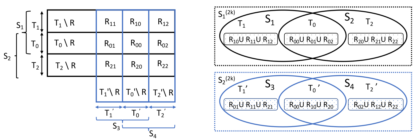
We remark that the value of $r_{ij}$ is naturally bounded by sample size in the corresponding overlapping set. For example, $r_{0*}=|(S_{1}\cap S_{2})\cap(S_{3}\cup S_{4})|\leq|(S_{1}\cap S_{2})|=d_{1}$ . Note that the 11 DoF of $\rho$ can also be illustrated by the left panel of Figure 4. There are 15 blocks but we have constraints $|S_{1}|=|S_{2}|=|S_{3}|=|S_{4}|=k$ , so we get $11=15-4$ DoF.

B.2 Discussion of Assumption 3

Assumption 3 reduces DoF of $\rho$ from 11 to 9, i.e., $\rho=\rho(\underline{r})$ . It drops 2 “within $S^{(2k)}_{1},S^{(2k)}_{2}$ overlapping” DoF $d_{1}$ and $d_{2}$ . The motivation is presented as follows. Given $c=|S^{(2k)}_{1}\cap S^{(2k)}_{2}|$ , $d_{1}$ and $d_{2}$ only describes the overlapping within $S^{(2k)}_{1}$ and $S^{(2k)}_{2}$ . Hence, these two DoF are expected to have smaller impact on $\rho={\mathrm{Cov}}[h(S_{1})h(S_{2}),h(S_{3})h(S-4)]$ than the other 9 DoF. This assumption can be validated in the following examples of linear average kernel.

Example 2.

Suppose $h$ is a linear average kernel, $h(X_{1},...,X_{k})=\frac{1}{k}\sum_{i=1}^{k}X_{i}$ , where $X_{1},...,X_{n}$ $i.i.d.~X$ , where ${\mathrm{E}}X=0,{\mathrm{E}}X^{2}=\mu_{2},{\mathrm{E}}X^{3}=\mu_{3},{\mathrm{E}}X^{4}=\mu_{4}$ . Notice that

\displaystyle{\mathrm{E}}(X_{1}X_{2}X_{3}X_{4})=\begin{cases}\mu_{2}^{2},&\text{if}\,X_{i}=X_{j},X_{k}=X_{l},X_{i}\neq X_{k},\,\text{where}\,\{i,j,k,l\}=\{1,2,3,4\};\\ \mu_{4},&\text{if}\,X_{1}=X_{2}=X_{3}=X_{4};\\ 0,&otherwise.\end{cases}

Hence, we have

\displaystyle{\mathrm{Cov}}(X_{1}X_{2},X_{3}X_{4})=\begin{cases}cov_{1}:=\mu_{2}^{2},&\text{if}\,X_{1}=X_{3}\neq X_{2}=X_{4};~or~X_{1}=X_{4}\neq X_{2}=X_{3};\\ cov_{2}:=\mu_{4}-\mu_{2}^{2},&\text{if}\,X_{1}=X_{2}=X_{3}=X_{4};\\ cov_{3}:=0,&otherwise.\end{cases}

Given the above 3 cases of ${\mathrm{Cov}}(X_{1}X_{2},X_{3}X_{4})$ , it is easy to verify that $\rho$ can be represented as a weighted average of $a_{1,n}cov_{1}+a_{2,n}cov_{2}+a_{3,n}cov_{3}$ , where $cov_{3}$ is 0. Moreover, by the definition of $cov_{1}$ and $cov_{2}$ , it is easy to verify that $a_{1,n}$ only depends on $r_{ij}$ for $(i,j)\neq(0,0)$ and $a_{2,n}$ only depends on $r_{0,0}$ . This verifies Assumption 3 on this linear average kernel. Besides, we can also show that $F^{(k)}$ in (31) (see Assumption 4) is a quadratic function of $c$ for this kernel.

In addition to the above example, the following discussion shows that we may not be able to further reduce the DoF from 9 to 4 by stronger assumptions. When ${\mathrm{E}}(h(S))=0$ , it is natural to consider the following fourth cumulant of $\rho$ :

	$\displaystyle cum_{4}[h(S_{1}),h(S_{2}),h(S_{3}),h(S_{4})]=$	$\displaystyle\rho-{\mathrm{Cov}}[h(S_{1}),h(S_{3})]{\mathrm{Cov}}[h(S_{2}),h(S_{4})]$
		$\displaystyle-{\mathrm{Cov}}[h(S_{1}),h(S_{4})]{\mathrm{Cov}}[h(S_{2}),h(S_{3})].$		(39)

If $cum_{4}[h(S_{1}),h(S_{2}),h(S_{3}),h(S_{4}))]$ in (B.2) is a lower order term of $\rho$ , the DoF can be reduced to 4, i.e., $|S_{1}\cap S_{3}|$ , $|S_{1}\cap S_{4}|$ , $|S_{2}\cap S_{3}|$ , and $|S_{2}\cap S_{4}|$ . However, Example 3 shows that this does not hold even for a linear average kernel.

Example 3.

Given size- $k$ sets $S_{1},S_{2},S_{3},S_{4}$ s.t. $S_{l}=(X_{1},Y_{1}^{(l)},...,Y_{k-1}^{(l)})$ , $X_{1},Y_{j}^{(l)}$ are i.i.d. $E(X_{1})=0,{\mathrm{Var}}(X_{1})>0$ , for $j=1,2,..,k-1$ and $l=1,2,3,4$ . By (B.2) and some direct calculations, we have $\rho=\frac{{\mathrm{Var}}(X_{1}^{2})}{k^{4}}$ , ${\mathrm{Cov}}[h(S_{1}),h(S_{3})]=\frac{{\mathrm{Var}}(X_{1})}{k^{2}}.$ Plugging in the above equations, we have

\displaystyle\frac{cum_{4}[h(X_{1}),h(X_{2}),h(X_{3}),h(X_{4})]}{2{\mathrm{Cov}}[h(S_{1}),h(S_{3})]^{2}}=\frac{{\mathrm{Var}}(X_{1}^{2})-2{\mathrm{Var}}^{2}(X_{1})}{2{\mathrm{Var}}^{2}(X_{1})}.

(40)

As long as ${\mathrm{Var}}(X_{1}^{2})-2{\mathrm{Var}}^{2}(X_{1})>0$ , which is common for non-Gaussian $X_{1}$ , Equation (40) is larger than $o(1)$ . This implies that the fourth cumulant is not always a lower order of $\rho$ .

We can further verify that given the kernel function is simple quadratic average kernel $h(S_{1})=h(X_{1},..,X_{k})=\frac{1}{k^{2}}[\sum_{i=1}^{k}X_{i}]^{2}$ , even if $X_{i}$ ’s are i.i.d. standard Gaussian, the fourth cumulant is still not a lower order term of $\rho$ ,.

B.3 Discussion of Assumption 4

In Equation (31), $F^{(k)}_{c}$ is defined as an upper bound for $\rho$ for a given $c$ . As illustrated by Figure 5: the more samples shared by $S_{1}$ and $S_{2}$ , $h(S_{1})h(S_{2})$ becomes closer to $h(S^{\prime})^{2}$ . Therefore, given that $|S^{(2k)}_{1}\cap S^{(2k)}_{2}|=c$ , $F_{c}$ has the most overlapping among all $\rho$ .

This assumption is trivial when considering the linear average kernel again: $h(S_{l})=\frac{1}{k}\sum_{i=1}^{k}X_{i}^{(l)}$ , for $l=1,2,3,4$ . In particular, considering $(S_{1},S_{2},S_{3},S_{4})$ s.t.

|S_{1}\cap S_{2}\cap S_{3}\cap S_{4}|=|(X_{1}^{(1)},...,X_{c}^{(1)})|=c

and $(S^{\prime},S^{\prime\prime})$ s.t. $|S^{\prime}\cap S^{\prime\prime}|=c$ , the equality in Equation (31) attains, i.e.,

\displaystyle\rho=k^{-4}{\mathrm{Var}}\left[(X_{1}^{(1)}+...+X_{c}^{(1)})^{2}\right]={\mathrm{Cov}}\left[h(S^{\prime})^{2},h(S^{\prime\prime})^{2}\right].

(41)

It is also straightforward to verify the assumption under simple quadratic average kernel function $h(S_{1})=\frac{1}{k^{2}}[\sum_{i=1}^{k}X_{i}]^{2}$

B.4 Discussion of Assumption 5

Assumption 2 shows a polynomial growth rate of the second moment term $\xi_{d,k}^{2}$ while Assumption 5 shows a polynomial growth rate of the fourth moment term $F^{(k)}$ . Assumption 5 also assumes $F_{1}^{(k)}$ is not a higher order term of $\xi_{1,k}^{4}$ . To better illustrate the idea of Assumption 5, we consider the following example with an oversimplified setting: the $cum_{4}$ term is 0 in Equation (B.2). Note that linear average kernel with i.i.d. standard Gaussian $X_{i}$ ’s satisfies this setting.

Example 4.

Suppose there is no fourth order cumulant term in Equation (B.2), by Equation (41), $F_{c}^{(k)}$ can be simplified as $\xi^{2}_{r_{22},k}\xi^{2}_{r_{22},k}+\xi^{2}_{r_{22},k}\xi^{2}_{r_{22},k}=2\xi_{r_{22},k}^{4}=2\xi_{c,k}^{4}$ . This also implies (32): $F_{1}^{(k)}/\xi_{1,k}^{4}={\cal O}(1)$ . We further remark that in this example, Assumption 5 can be implied by Assumption 2. To be more specific, as demonstrated in the following equation, $a_{2}$ in (33) is $2a_{1}$ , where $a_{1}$ is provided in Assumption 2.

\displaystyle\frac{F_{c}^{(k)}}{F_{1}^{(k)}}=\frac{2\xi_{c,k}^{4}}{\xi_{1,k}^{4}}=2\left(\frac{\xi_{c,k}^{2}}{\xi_{1,k}^{2}}\right)^{2}={\cal O}(c^{2a_{1}}),\,\text{for}\,c=1,2,...,k.

(42)

By Lemma F.3 (see Appendix F), a natural upper bound for $\sigma_{c,2k}^{2}$ is $F_{c}^{(k)}$ (31). Hence, even if $\xi_{d,k}^{2}$ has a linear growth rate regarding $d$ , $F^{(k)}$ still can growth at a quadratic rate of $c$ (see (42)). Therefore, we cannot assume $\sigma_{2k,2k}^{2}/(2k\sigma_{1,2k}^{2})={\cal O}(1)$ ., which is the common assumption on the counterpart $\xi_{1,2k}^{2}$ [16, 30, 6]. That is one reason that Assumptions 3-5 are imposed on the primitive term $\rho$ instead of on $\sigma_{c,2k}^{2}$ .

Appendix C Proof of Main Results

C.1 Proof of Corollary 4.6

To show $\frac{\hat{V}_{u}}{E(\hat{V}_{u})}\xrightarrow{P}1$ as $n\to\infty$ , it suffice to show the $L_{2}$ convergence of $\hat{V}_{u}/E(\hat{V}_{u})$ , i.e., ${\mathrm{Var}}(\hat{V}_{u})/\left({\mathrm{E}}(\hat{V}_{u})\right)^{2}\to 0$ as $n\to\infty$ .

By plugging Equation (34) and (35) from Theorem 4.4, we have

\displaystyle\frac{{\mathrm{Var}}(\hat{V}_{u})}{\left({\mathrm{E}}(\hat{V}_{u})\right)^{2}}=\frac{{\cal O}\left(\frac{k^{2}}{n}\check{\sigma}_{1,2k}^{2}\right)}{\left[\left(1+o(1)\right)\frac{k^{2}}{n}\xi_{1,k}^{2}\right]^{2}}={\cal O}\left(\frac{n}{k^{2}}\frac{\check{\sigma}_{1,2k}^{2}}{\xi_{1,k}^{4}}\right),

(43)

where $\check{\sigma}_{1,2k}^{2}\asymp\frac{k^{2}}{n^{2}}F^{(k)}_{1}$ is the upper bound of $\sigma_{1,2k}^{2}$ given by Proposition F.2. By Assumption 5, $F^{(k)}_{1}={\cal O}(\xi_{1,k}^{4})$ . Plugging $\check{\sigma}_{1,2k}^{2}$ into Equation (43), we conclude that

\displaystyle\frac{{\mathrm{Var}}(\hat{V}_{u})}{\left({\mathrm{E}}(\hat{V}_{u})\right)^{2}}={\cal O}\left(\frac{1}{n}\right).

∎

C.2 Proof of Theorem 4.4

We first present a technical proposition to be used soon.

Proposition C.1.

For any integer $c$ , s.t. $1\leq c\leq k$ and $k=o(\sqrt{n})$ ,

\displaystyle\binom{n}{k}^{-1}\binom{k}{c}\binom{n-k}{k-c}\leq\frac{1}{c!}\left(\frac{k^{2}}{n-k-1}\right)^{c}.

This proof is provided by DiCiccio and Romano 2022. We first write the combinatorial numbers as factorial numbers

	$\displaystyle\binom{n}{k}^{-1}\binom{k}{c}\binom{n-k}{k-c}$	$\displaystyle=\frac{(n-k)!k!}{n!}\frac{k!}{(k-c)!c!}\frac{(n-k)!}{(k-c)!(n-2k+c)!}$
		$\displaystyle=\frac{1}{c!}\left[\frac{k!k!}{(k-c)!(k-c)!}\right]\left[\frac{(n-k)!(n-k!)}{n!(n-2k+c)!}\right].$		(44)

It suffices to upper bound things inside two square brackets separately. We have

\displaystyle\left[\frac{k!k!}{(k-c)!(k-c)!}\right]\leq k^{2c},

(45)

\displaystyle\frac{(n-k)!(n-k!)}{n!(n-2k+c)!}=\frac{(n-k)(n-k-1)...(n-2k+c+1))}{n(n-1)...(n-k+1)}\leq\left[\frac{1}{n-k+1}\right]^{c}.

(46)

Combining (45) and (46) into (44), we completes the proof. ∎

First, we show Equation (34). By Proposition 4.5 and Assumption 2, we can conclude that

\displaystyle\lim_{n\to\infty}\frac{{\mathrm{Var}}(U_{n})}{\frac{k^{2}}{n}\xi_{1,k}^{2}}=1.

Secondly, we show Equation (35).

$\displaystyle{\mathrm{Var}}(\hat{V}_{u})\asymp{\mathrm{Var}}^{(T_{1})}(\hat{V}_{u})=$	$\displaystyle\sum_{c=1}^{T_{1}}\binom{n}{2k}^{-1}\binom{2k}{c}\binom{n-2k}{2k-c}\sigma_{c,2k}^{2}$	(47)
$\displaystyle=$	$\displaystyle\sum_{c=1}^{T_{1}}\binom{n}{2k}^{-1}\binom{2k}{c}\binom{n-2k}{2k-c}{\cal O}(\frac{k^{2}}{n^{2}}F_{c}^{(k)})$	(48)
$\displaystyle=$	$\displaystyle\sum_{c=1}^{T_{1}}{\cal O}(\frac{k^{2c+2}}{n^{c+2}}F_{c}^{(k)})$	(49)
$\displaystyle=$	$\displaystyle{\cal O}(\frac{k^{4}}{n^{3}}F_{1}^{(k)}).$	(50)

Here, (47) is concluded by Lemma F.4. (48) is concluded by $\sigma_{c,2k}^{2}={\cal O}(\frac{k^{2}}{n^{2}}F_{c}^{(k)})$ (Proposition F.2). (49) is concluded by $\binom{n}{2k}^{-1}\binom{2k}{c}\binom{n-2k}{2k-c}=[1+o(1)]\frac{k^{2c}}{n^{c}}$ for $c=1,2,...,T_{1}$ (Proposition C.1). (50) is concluded by the bounded growth rate of $F^{(k)}$ in Assumption 5 and finite $T_{1}$ . If we denote $\frac{k^{2}}{n^{2}}F_{1}^{(k)}$ as $\widecheck{\sigma}_{1,2k}^{2}$ , we conclude that ${\mathrm{Var}}(\hat{V}_{u})={\cal O}(\frac{k^{2}}{n}\widecheck{\sigma}_{1,2k}^{2})$ . ∎

C.3 Proof of Proposition 4.5

For $k=o(\sqrt{n})$ , we want to show $\lim_{n\to\infty}\frac{{\mathrm{Var}}(U_{n})}{\frac{k^{2}}{n}\xi_{1,k}^{2}}=1$ . First notice that for the coefficient leading term $\binom{n}{k}^{-1}\binom{k}{1}\binom{n-k}{k-1}\xi_{1,k}^{2}$ , we have

\displaystyle\frac{\binom{n}{k}^{-1}\binom{k}{1}\binom{n-k}{k-1}}{\frac{k^{2}}{n}}=\frac{(n-k)!(n-k)!}{(n-1)!(n-2k+1)!}\rightarrow 1,\,\text{as $n\rightarrow\infty$.}

(51)

Therefore, it suffices to show that the rest part of ${\mathrm{Var}}(U_{n})$ is dominated by the leading term:

\displaystyle\lim_{n\to\infty}\frac{\binom{n}{k}^{-1}\sum_{d=2}^{k}\binom{k}{d}\binom{n-k}{k-d}\xi^{2}_{d,k}}{\frac{k^{2}}{n}\xi_{1,k}^{2}}=0.

By Proposition C.1, the numerator of the above can be bounded as

\displaystyle\binom{n}{k}^{-1}\sum_{d=2}^{k}\binom{k}{d}\binom{n-k}{k-d}\xi^{2}_{d,k}\leq\sum_{d=2}^{k}\frac{k^{2d}}{d!(n-k+1)^{d}}\xi_{d,k}^{2}:\sum_{d=2}^{k}(d!)^{-1}b_{n}^{d}\xi_{d,k}^{2},

(52)

where $b_{n}=\frac{k^{2}}{n-k-1}$ . Notice that $n<2(n-k+1)$ , so we have

\displaystyle\frac{\binom{n}{k}^{-1}\sum_{d=2}^{k}\binom{k}{d}\binom{n-k}{k-d}\xi^{2}_{d,k}}{\frac{k^{2}}{n}\xi_{1,k}^{2}}\leq\frac{n}{n-k+1}\sum_{d=2}^{k}\frac{1}{d!}b_{n}^{d-1}\frac{\xi_{d,k}^{2}}{\xi_{1,k}^{2}}\leq\sum_{d=2}^{k}\frac{2}{d!}b_{n}^{d-1}\frac{\xi_{d,k}^{2}}{\xi_{1,k}^{2}}.

(53)

By Assumption 2, the growth rate of $\xi_{d,k}^{2}$ is bounded, there exists a uniform constant $C$ s.t. $\frac{\xi_{d,k}^{2}}{\xi_{1,k}^{2}}\leq Cd!$ for $d=2,3,...,k$ . Therefore, the RHS of Equation (53) is bounded as

\displaystyle\sum_{d=2}^{k}\frac{1}{d!}b_{n}^{d-1}\frac{\xi_{d,k}^{2}}{\xi_{1,k}^{2}}\leq\sum_{d=2}^{k}\frac{1}{d!}b_{n}^{d-1}\frac{Cd!\xi_{1,k}^{2}}{\xi_{1,k}^{2}}\leq C\sum_{d=2}^{k}b_{n}^{d-1}=Cb_{n}\frac{1-b_{n}^{k-1}}{1-b_{n}}\leq C\frac{b_{n}}{1-b_{n}}.

(54)

The RHS of (54) goes to 0 when $n\to\infty$ , since $b_{n}=\frac{k^{2}}{n-k-1}\to 0$ . This completes the proof.

∎

Appendix D Proof of Double U-Statistics

D.1 Proof of Proposition 4.2

Proof of Equation (23).

We first show the following equation.

\displaystyle\psi\left(S^{(2k)}\right)=\sum_{d=0}^{k}w_{d}\varphi_{d}\left(S^{(2k)}\right)

(55)

Wang and Lindsay 2014 have demonstrated that $\hat{V}_{u}$ is an U-statistic with size-2k kernel (Equation (19)):

\displaystyle\hat{V}_{u}=Q(k)-Q(0)=\binom{n}{2k}^{-1}\sum_{S^{(2k)}\subseteq\mathcal{X}_{n}}\left[\psi_{k}\left(S^{(2k)}\right)-\psi_{0}\left(S^{(2k)}\right)\right],

		$\displaystyle\psi_{k}\left(S^{(2k)}\right)=\underbrace{\binom{n}{2k}\binom{n}{k}^{-1}\binom{n}{k}^{-1}}_{A_{1}}\sum_{d=0}^{k}\frac{1}{N_{d}}\sum_{\begin{subarray}{c}S_{1},S_{2}\subset S^{(2k)}\\ \|S_{1}\cap S_{2}\|=d\end{subarray}}h\left(S_{1}\right)h\left(S_{2}\right),$
		$\displaystyle\psi_{0}\left(S^{(2k)}\right)=\underbrace{\binom{n}{2k}\binom{n}{k}^{-1}\binom{n-k}{k}^{-1}}_{A_{1,0}}\frac{1}{N_{0}}\sum_{\begin{subarray}{c}S_{1},S_{2}\subset S^{(2k)}\\ \|S_{1}\cap S_{2}\|=0\end{subarray}}h\left(S_{1}\right)h\left(S_{2}\right),$

where $N_{d}=\binom{n-2k+d}{d}$ .

Denote

\displaystyle A_{1}:=\binom{n}{2k}\binom{n}{k}^{-2},\quad A_{1,0}:=\binom{n}{2k}\binom{n}{k}^{-1}\binom{n-k}{k}^{-1}.

(56)

Rewrite $\psi_{k}\left(S^{(2k)}\right)-\psi_{0}\left(S^{(2k)}\right)$ by the order of $d$ . Notice that there is a $\sum_{d=0}^{k}$ in $\psi_{k}\left(S^{(2k)}\right)$ but $d$ can only be $0$ in $\psi_{0}\left(S^{(2k)}\right)$ . Hence, there is a cancellation for $h(S_{1})h(S_{2})$ s.t. $d=|S_{1}\cap S_{2}|=0$ , thus we have

\displaystyle\psi_{k}\left(S^{(2k)}\right)-\psi_{0}\left(S^{(2k)}\right)=

\displaystyle A_{1}\sum_{d=1}^{k}\frac{1}{N_{d}}\sum_{\begin{subarray}{c}S_{1},S_{2}\subset S^{(2k)}\\ |S_{1}\cap S_{2}|=d\end{subarray}}h\left(S_{1}\right)h\left(S_{2}\right)+(A_{1}-A_{1,0})\frac{1}{N_{0}}\sum_{\begin{subarray}{c}S_{1},S_{2}\subset S^{(2k)}\\ |S_{1}\cap S_{2}|=0\end{subarray}}h\left(S_{1}\right)h\left(S_{2}\right).

For the RHS of above equation, multiply and divide $M_{d,k}$ (24) inside $\sum_{d=1}^{k}$ :

\displaystyle\begin{split}\psi_{k}\left(S^{(2k)}\right)-\psi_{0}\left(S^{(2k)}\right)=&\sum_{d=1}^{k}\underbrace{\left[A_{1}\frac{1}{N_{d}}M_{d,k}\right]}_{w_{d}}\underbrace{\frac{1}{M_{d,k}}\sum_{S_{1},S_{2}\subset S^{(2k)},\,|S_{1}\cap S_{2}|=d}h\left(S_{1}\right)h\left(S_{2}\right)}_{\varphi_{d}(S^{(2k)})}\\ &+\underbrace{\left[(A_{1}-A_{1,0})\frac{1}{N_{0}}M_{0,k}\right]}_{w_{0}}\underbrace{\frac{1}{M_{0,k}}\sum_{S_{1},S_{2}\subset S^{(2k)},\,|S_{1}\cap S_{2}|=0}h\left(S_{1}\right)h\left(S_{2}\right)}_{\varphi_{0}(S^{(2k)})}.\end{split}

We denote

		$\displaystyle w_{d}:=\frac{A_{1}}{N_{d}}M_{d,k},\quad\text{for }d=1,2,...,k;$
		$\displaystyle w_{0}:=\frac{(A_{1}-A_{1,0})M_{0,k}}{N_{0}};$
		$\displaystyle\varphi_{d}(S^{(2k)}):=\frac{1}{M_{d,k}}\sum_{\begin{subarray}{c}S_{1},S_{2}\subset S^{(2k)}\\ \|S_{1}\cap S_{2}\|=d\end{subarray}}h\left(S_{1}\right)h\left(S_{2}\right),\quad\text{for }d=1,2,...,k;$
		$\displaystyle\varphi_{0}(S^{(2k)}):=\frac{1}{M_{0,k}}\sum_{\begin{subarray}{c}S_{1},S_{2}\subset S^{(2k)}\\ \|S_{1}\cap S_{2}\|=0\end{subarray}}h\left(S_{1}\right)h\left(S_{2}\right).$

Thus we have

\displaystyle\psi_{k}\left(S^{(2k)}\right)-\psi_{0}\left(S^{(2k)}\right)=\left[\sum_{d=1}^{k}w_{d}\varphi_{d}(S^{(2k)})\right]+w_{0}\varphi_{0}(S^{(2k)})=\sum_{d=0}^{k}w_{d}\varphi_{d}(S^{(2k)}).

Given that $\sum_{d=0}^{k}w_{d}=0$ is true (to be proved soon), then $w_{0}=-\sum_{d=1}^{k}w_{d}$ . Therefore,

\displaystyle\begin{split}\psi\left(S^{(2k)}\right)&=\sum_{d=0}^{k}w_{d}\varphi_{d}\left(S^{(2k)}\right)=\sum_{d=1}^{k}w_{d}\varphi_{d}\left(S^{(2k)}\right)-\left(\sum_{d=1}^{k}w_{d}\right)\varphi_{0}\left(S^{(2k)}\right)\\ &=\sum_{d=1}^{k}w_{d}\left[\varphi_{d}\left(S^{(2k)}\right)-\varphi_{0}\left(S^{(2k)}\right)\right].\end{split}

Proof of Equation Equation (25)

First, we show that $\sum_{d=0}^{k}w_{d}=0$ . As discussed above, $w_{d}$ is a product of three normalization constants: $A_{1}=\binom{n}{2k}\binom{n}{k}^{-2}$ and $A_{1,0}=\binom{n}{2k}\binom{n}{k}^{-1}\binom{n-k}{k}^{-1}$ are the normalization constant to rewrite $Q(k)$ and $Q(0)$ as a U-statistic; $M_{d,k}:=\binom{2k}{d}\binom{2k-d}{d}\binom{2k-2d}{k-d}$ is the number of pairs $S_{1},S_{2}\subset S^{(2k)}$ s.t. $|S_{1}\cap S_{2}|=d$ ; $N_{d}=\binom{n-2k+d}{d}$ is defined in Equation (20).

\displaystyle w_{0}=\frac{(A_{1}-A_{1,0})M_{0,k}}{N_{0}};\,\,w_{d}=\frac{A_{1}M_{d,k}}{N_{d}},\quad\text{for }d=1,2,...,k.

Since $A_{1,0}>A_{1}>0$ , $M_{d,k}>0$ , $N_{d}>0$ , we have $w_{d}>0,\forall d\geq 1$ and $w_{0}<0$ . Then we show $\sum_{d=0}^{k}w_{d}=0$ . Though this can be justified by direct calculation, we present a more intuitive proof. Recall $\hat{V}_{u}=Q(k)-Q(0)$ . By the definition of $Q(k)$ , $Q(k)$ can be represented as a weighted sum of $h(S_{1})h(S_{2})$ , i.e., $\sum_{1\leq i,j\leq n}a_{ij}h(S_{i})h(S_{j})$ , where $\sum_{1\leq i<j\leq n}a_{ij}=1$ . Thus, $Q(k)-Q(0)$ can be represented in a similar way:

\displaystyle Q(k)-Q(0)=\sum_{1\leq i<j\leq n}a_{ij}^{\prime}h(S_{i})h(S_{j}),

where $\sum_{1\leq i,j\leq n}a_{ij}^{\prime}=0$ . Therefore $\psi_{k}\left(S^{(2k)}\right)-\psi_{0}\left(S^{(2k)}\right)$ , as the kernel of U-statistic $Q(k)-Q(0)$ , can also be represented in the form of a weighted sum:

\displaystyle\psi_{k}\left(S^{(2k)}\right)-\psi_{0}\left(S^{(2k)}\right)=\sum_{1\leq i<j\leq n}b_{ij}h(S_{i})h(S_{j}),

(57)

where $\sum_{1\leq i<j\leq n}b_{ij}=0$ since $\psi_{k}\left(S^{(2k)}\right)-\psi_{0}\left(S^{(2k)}\right)$ is an unbiased estimator of $Q(k)-Q(0)$ . On the other hand, for $d=0,1,2,...,k$ , $\varphi_{d}(S^{(2k)})$ is still a U-statistic, which can be represented in the form of a weighted sum:

\displaystyle\varphi_{d}\left(S^{(2k)}\right)=\sum_{1\leq i<j\leq n}c_{ij}^{(d)}h(S_{i})h(S_{j}),

(58)

where $\sum_{1\leq i<j\leq n}c_{ij}^{(d)}=1$ . Since $\psi_{k}\left(S^{(2k)}\right)-\psi_{0}\left(S^{(2k)}\right)=\sum_{d=0}^{k}w_{d}\varphi_{d}\left(S^{(2k)}\right)$ , by comparing Equation (57) and (58), we have $\sum_{d=1}^{k}w_{d}\sum_{1\leq i<j\leq n}c_{ij}^{(d)}=\sum_{1\leq i<j\leq n}b_{ij}$ . Since $\sum_{1\leq i<j\leq n}c_{ij}^{(d)}=1$ and $\sum_{1\leq i<j\leq n}b_{ij}=0$ , we can take $h(S_{i})=1$ for $i=1,2,...,n$ and conclude that

\displaystyle\sum_{d=0}^{k}w_{d}=0.

Secondly, we present the details to bound $w_{d}=A_{1}M_{d,k}/N_{d}$ , for $d=1,2,...,k$ . Plug in the expression of $A_{1},M_{d,k},N_{d}$ , we have

	$\displaystyle w_{d}=$	$\displaystyle\left[\binom{n}{2k}\binom{n}{k}^{-2}\right]\left[\binom{2k}{d}\binom{2k-d}{d}\binom{2k-2d}{k-d}\right]/\binom{n-2k+d}{d}$
	$\displaystyle=$	$\displaystyle\left[\frac{n!}{(n-2k)!(2k)!}\frac{(n-k)!(n-k)!k!k!}{n!n!}\right]\left[\frac{(2k)!(2k-d)!(2k-2d)!}{(2k-d)!d!(2k-2d)!d!(k-d)!(k-d)!}\right]\left[\frac{d!(n-2k)!}{(n-2k+d)!}\right].$

After direct cancellation of the same factorials, we have

\displaystyle w_{d}=\underbrace{\frac{(n-k)!(n-k)!}{n!(n-2k+d)!}}_{\text{Part I}}\underbrace{\frac{k!k!}{(k-d)!(k-d)!}}_{\text{part II}}\underbrace{\frac{1}{d!}}_{\text{part III}}.

(59)

For Part I in (59),

\displaystyle\frac{(n-k)!(n-k)!}{n!(n-2k+d)!}=\frac{\prod_{i=0}^{k-d-1}(n-k-i)}{\prod_{i=0}^{k-1}(n-i)}=[1+o(1)]\frac{1}{n^{d}}.

The last equality is because for any $k=o(\sqrt{n}),d\leq k$ , we have

\displaystyle\frac{\prod_{i=0}^{k-d-1}(n-k-i)}{\prod_{i=0}^{k-1}(n-i)}\leq\frac{\prod_{i=0}^{k-d-1}(n-i)}{\prod_{i=0}^{k-1}(n-i)}=\frac{1}{\prod_{i=0}^{d-1}(n-k+d-i)}\leq\frac{1}{(n-k)^{d}}=[1+o(1)]\frac{1}{n^{d}}.

On the other hand,

\displaystyle\frac{\prod_{i=0}^{k-d-1}(n-k-i)}{\prod_{i=0}^{k-1}(n-i)}\geq\frac{1}{n^{d}}.

Combining $\leq$ and $\geq$ , we have $=[1+o(1)]\frac{1}{n^{d}}$ . For Part II (59),

\displaystyle\frac{k!k!}{(k-d)!(k-d)!}=[k(k-1)...(k-d+1)]^{2}]\leq k^{2d}.

Particularly, when $d$ is fixed, we have $\frac{k!k!}{(k-d)!(k-d)!}=k(k-1)...(k-d+1)]^{2}=[1+o(1)]k^{2d}$ . Combining Part I, II, III in (59), we have

\displaystyle w_{d}=\begin{cases}[1+o(1)]\left[\frac{1}{d!}(\frac{k^{2}}{n})^{d}\right]&\forall\text{ finite $d$;}\\ {\cal O}\left[\frac{1}{d!}(\frac{k^{2}}{n})^{d}\right]&\forall d=1,2,...,k.\end{cases}

∎

Appendix E Proof of Results in Methodology Section

E.1 Variance of Incomplete U-statistics $U_{n,B,M}$

This is an extension of the results by Wang 2012 and Wang and Lindsay 2014.

Comparing ${\mathrm{Var}}(U_{n,B,M})=(1-\frac{1}{B})Var(U_{n})+\frac{1}{MB}V^{(h)}$ (14) with ${\mathrm{Var}}(U_{n,B})={\mathrm{Var}}(U_{n})+{\mathrm{E}}[{\mathrm{Var}}(U_{n,B}|{\cal X}_{n})]$ (5) , it suffices to show that

\displaystyle{\mathrm{E}}\left[{\mathrm{Var}}(U_{n,B}|{\cal X}_{n})\right]=\frac{1}{MB}V^{(h)}-\frac{1}{B}{\mathrm{Var}}(U_{n}).

Here we adopt an alternative view of a complete U-statistic $U_{n}$ with $k\leq n/2$ by Wang and Lindsay 2014. Follow our notation of “matched group”, we can always take $M=\left\lfloor n/k\right\rfloor$ mutually disjoint subsamples $S_{1},...,S_{M}$ from $(X_{1},...,X_{n})$ , such that $|S_{i}\cap S_{j}|=0$ for $1\leq i<j\leq M$ . Wang and Lindsay 2014 take integer $M=n/k$ while we allow $2\leq M\leq\left\lfloor n/k\right\rfloor$ . Recall such $(S_{1}^{(b)},...,S_{M}^{(b)})$ as a “matched group”, where $b$ is the index of group. Let ${\cal G}_{n,k,M}$ be the collection of all such matched groups constructed from $n$ samples, i.e.,

\displaystyle{\cal G}_{n,k,M}=\big\{(S_{1}^{(b)},\ldots,S_{M}^{(b)}):\cup_{j}S_{j}^{(b)}\subset{\cal X}_{n},\,\,\text{and}\,\,S_{i}^{(b)}\cap S_{j}^{(b)}=\emptyset,\forall 1\leq i,j\leq M\big\}.

(60)

Then, an alternative representation of $U_{n}$ is

\displaystyle U_{n}=\frac{1}{M|{\cal G}_{n,k,M}|}\sum_{b=1}^{|{\cal G}_{n,k,M}|}\sum_{i=1}^{M}S_{i}^{(b)}.

(61)

This form seems redundant because there are some replicate subsample among all $S_{i}^{(b)}$ ’s. However, for incomplete U-statistic $U_{n,B,M}$ , each $(S_{1}^{(b)},...,S_{M}^{(b)})$ can be viewed as a sample from ${\cal G}_{n,k,M}$ . Hence, Wang 2012 show that $B\cdot{\mathrm{Var}}(U_{n,B}|{\cal X}_{n})=\frac{1}{|{\cal G}_{n,k,M}|}\sum_{b=1}^{|{\cal G}_{n,k,M}|}(\bar{h}^{(b)}-U_{n})^{2}$ , where $\bar{h}^{(b)}=\frac{1}{M}\sum_{i=1}^{M}h(S_{i}^{(b)})$ , $S_{i}^{(b)}$ ’s are all subsamples associated with the complete U-statistic $U_{n}$ on ${\cal X}$ . However, Wang 2012 and Wang and Lindsay 2014 do not provide a simple expression in the form of $V^{(h)}$ and ${\mathrm{Var}}(U_{n})$ . We further simplify $B{\mathrm{Var}}(U_{n,B}|{\cal X}_{n})$ as follows,

	$\displaystyle B\cdot{\mathrm{E}}\left[{\mathrm{Var}}(U_{n,B}\|{\cal X}_{n})\right]=$	$\displaystyle{\mathrm{E}}\left(\frac{1}{\|{\cal G}_{n,k,M}\|}\sum_{b=1}^{\|{\cal G}_{n,k,M}\|}(\bar{h}^{(b)}-U_{n})^{2}\right)$
	$\displaystyle=$	$\displaystyle{\mathrm{E}}\left[\frac{1}{\|{\cal G}_{n,k,M}\|}\sum_{b=1}^{\|{\cal G}_{n,k,M}\|}\left((\bar{h}^{(b)}-{\mathrm{E}}(U_{n}))-(U_{n}-{\mathrm{E}}(U_{n}))\right)^{2}\right]$
	$\displaystyle=$	$\displaystyle\frac{1}{\|{\cal G}_{n,k,M}\|}\left[\sum_{b=1}^{\|{\cal G}_{n,k,M}\|}{\mathrm{E}}\left(\left(\bar{h}^{(b)}-{\mathrm{E}}(U_{n})\right)^{2}\right)\right]+\frac{1}{\|{\cal G}_{n,k,M}\|}\left[\sum_{b=1}^{\|{\cal G}_{n,k,M}\|}{\mathrm{E}}\left(\left(U_{n}-{\mathrm{E}}(U_{n})\right)^{2}\right)\right]$
		$\displaystyle-2{\mathrm{E}}\left(\frac{1}{\|{\cal G}_{n,k,M}\|}\sum_{b=1}^{\|{\cal G}_{n,k,M}\|}(\bar{h}^{(b)}-{\mathrm{E}}(U_{n}))(U_{n}-{\mathrm{E}}(U_{n})\right)$
	$\displaystyle=$	$\displaystyle{\mathrm{Var}}\left(\bar{h}^{(1)}\right)-{\mathrm{Var}}(U_{n})$
	$\displaystyle=$	$\displaystyle\frac{1}{M}V^{(h)}-{\mathrm{Var}}(U_{n}).$

In the above equations, the first equality is the conclusion by Wang 2012; the next-to-last equality holds since $\frac{1}{|{\cal G}_{n,k,M}|}\sum_{b=1}^{|{\cal G}_{n,k,M}|}\bar{h}^{(b)}=U_{n}$ ; the last equality holds since $h(S_{1}^{(1)}),...,h(S_{M}^{(1)})$ are independent.

∎

E.2 Unbiasedness of Variance Estimators

First, we restrict the discussion given $k\leq n/2$ . We first show that $\hat{V}^{(s)}=\sum_{d=0}^{k}\gamma_{d,k,n}\hat{\tilde{\xi}}_{d,k}^{2}$ . By the discussion in Section 3.3.1, we have $N_{d,k,n}=\binom{n}{k}^{2}\gamma_{d,k,n}$ . For a complete U-statistic with $k\leq n/2$ , $N_{d,k,n}=\binom{n}{k}\binom{n-k}{k-d}\binom{k}{d}$ and we denote $\mathbbm{N}=\binom{n}{k}>0$ . Then,

	$\displaystyle\sum_{d=0}^{k}\gamma_{d,k,n}\hat{\tilde{\xi}}_{d,k}^{2}=$	$\displaystyle\sum_{d=0}^{k}\mathbbm{N}^{-2}N_{d,k,n}\hat{\tilde{\xi}}_{d,k}^{2}$
	$\displaystyle=$	$\displaystyle\mathbbm{N}^{-2}\sum_{1\leq i\leq\mathbbm{N}}\sum_{1\leq j\leq\mathbbm{N}}\sum_{d=0}^{k}\mathbbm{1}\{{\|S_{i}\cap S_{j}\|=d}\}[h(S_{i})-h(S_{j})]^{2}/2$
	$\displaystyle=$	$\displaystyle\mathbbm{N}^{-2}\left[2\sum_{1\leq i<j\leq\mathbbm{N}}\sum_{d=0}^{k-1}\mathbbm{1}\{{\|S_{i}\cap S_{j}\|=d}\}[h(S_{i})-h(S_{j})]^{2}/2\right]$
	$\displaystyle=$	$\displaystyle\frac{\mathbbm{N}(\mathbbm{N}-1)}{\mathbbm{N}^{2}}\left[\binom{\mathbbm{N}}{2}^{-1}\sum_{1\leq i<j\leq\mathbbm{N}}[h(S_{i})-h(S_{j})]^{2}/2\right]$
	$\displaystyle=$	$\displaystyle\frac{\mathbbm{N}-1}{\mathbbm{N}}\left[\frac{1}{\mathbbm{N}-1}\sum_{i=1}^{\mathbbm{N}}[h(S_{i})-U_{n}]^{2}\right]$
	$\displaystyle=$	$\displaystyle\frac{1}{\mathbbm{N}}\sum_{i=1}^{\mathbbm{N}}[h(S_{i})-U_{n}]^{2}=\hat{V}^{(s)}$

Here, the second equality holds by plugging in the definition of $N_{d,k,n}$ and interchanging the finite summation $\sum_{d\in{\cal D}}$ with $\sum_{1\leq i<j\leq B}$ . The third equality omits the cases with $i=j$ , where $h(S_{i})-h(S_{j})=0$ . The second to last equality holds because the sample variance is essentially an order-2 U-statistic, with kernel $(h(S_{i})-h(S_{j}))^{2}/2$ .

Then, as we demonstrated in Section 3.3.1, ${\mathrm{E}}(\hat{\tilde{\xi}}_{d,k}^{2})=\tilde{\xi}_{d,k}^{2}$ for $d=0,1,...,k$ . Hence we conclude that

\displaystyle{\mathrm{E}}\left(\hat{V}^{(s)}\right)=\sum_{d=0}^{k}\gamma_{d,k,n}{\mathrm{E}}\left(\hat{\tilde{\xi}}_{d,k}^{2}\right)=\sum_{d=0}^{k}\gamma_{d,k,n}\tilde{\xi}_{d,k}^{2}=V^{(s)}.

Secondly, we extend the previous argument to the setting $n/2<k<n$ . We denote ${\cal D}=\{d\in N^{*}|0\leq d\leq k,\gamma_{d,k,n}>0\}$ . We can define $\hat{V}^{(s)}=\sum_{d\in{\cal D}}\gamma_{d,k,n}\hat{\tilde{\xi}}_{d,k}^{2}$ . We want to show that

	$\displaystyle\hat{V}^{(s)}=\frac{1}{\mathbbm{N}}\sum_{i=1}^{\mathbbm{N}}[h(S_{i})-U_{n}]^{2},$		(62)
	$\displaystyle{\mathrm{E}}(\hat{V}^{(s)})=V^{(s)}.$		(63)

Similar to previous proof

	$\displaystyle\hat{V}^{(S)^{\prime}}=$	$\displaystyle\sum_{d\in{\cal D}}\mathbbm{N}^{-2}N_{d,k,n}\hat{\tilde{\xi}}_{d,k}^{2}$
	$\displaystyle=$	$\displaystyle\mathbbm{N}^{-2}\left[2\sum_{1\leq i<j\leq\mathbbm{N}}\sum_{d\in{\cal D}\backslash\{k\}}\mathbbm{1}\{{\|S_{i}\cap S_{j}\|=d}\}[h(S_{i})-h(S_{j})]^{2}/2\right]$
	$\displaystyle=$	$\displaystyle\frac{\mathbbm{N}(\mathbbm{N}-1))}{\mathbbm{N}^{2}}\left[\binom{\mathbbm{N}}{2}^{-1}\sum_{1\leq i<j\leq\mathbbm{N}}[h(S_{i})-h(S_{j})]^{2}/2\right]$
	$\displaystyle=$	$\displaystyle\frac{\mathbbm{N}-1}{\mathbbm{N}}\left[\frac{1}{\mathbbm{N}-1}\sum_{i=1}^{\mathbbm{N}}[h(S_{i})-U_{n}]^{2}\right]$
	$\displaystyle=$	$\displaystyle\frac{1}{\mathbbm{N}}\sum_{i=1}^{\mathbbm{N}}[h(S_{i})-U_{n}]^{2}$

Since each $\hat{\tilde{\xi}}_{d,k}^{2}$ is still an unbiased estimator of $\tilde{\xi}_{d,k}^{2}$ , similarly, we have ${\mathrm{E}}(\hat{V}^{(S)^{\prime}})=V^{(s)}$ . Remark that the summation in Equation (62) is over $d\in{\cal D}$ instead of $d=0,1,2,...,n$ . This is because $\gamma_{d,k,n}$ is 0 for small $d$ , given $k>n/2$ . In other words, when $k>n/2$ , several terms of $\gamma_{d,k,n}\xi_{d,k}^{2}$ in the Hoeffding decomposition (2) is already 0.

∎

Since a sample variance is an order-2 U-statistics,

	$\displaystyle\hat{V}_{B,M}^{(s)}=$	$\displaystyle[(BM-1)BM]^{-1}\sum_{i=1}^{M}\sum_{j=1}^{B}\sum_{(i^{\prime},j^{\prime})\neq(i,j)}\left[h(S_{i}^{(j)})-h(S_{i^{\prime}}^{(j^{\prime})})\right]^{2}/2$
	$\displaystyle=$	$\displaystyle[(BM-1)BM]^{-1}\sum_{i=1}^{M}\sum_{j=1}^{B}\left(\sum_{(i^{\prime},j^{\prime})\in{\cal A}(i,j)}+\sum_{(i^{\prime},j^{\prime})\in{\cal B}(i,j)}\right)\left[h(S_{i}^{(j)})-h(S_{i^{\prime}}^{(j^{\prime})})\right]^{2}/2$
	$\displaystyle:=$	$\displaystyle[(BM-1)BM]^{-1}\sum_{i=1}^{M}\sum_{j=1}^{B}\left(\sum_{(i^{\prime},j^{\prime})\in{\cal A}(i,j)}+\sum_{(i^{\prime},j^{\prime})\in{\cal B}(i,j)}\right)\hat{v}_{(i,j,i^{\prime},j^{\prime})},$

where ${\cal A}(i,j)=\{(i^{\prime},j^{\prime})|i^{\prime}\neq i,j^{\prime}=j,1\leq i^{\prime}\leq M,1\leq j^{\prime}\leq B\}$ ; ${\cal B}(i,j)=\{(i^{\prime},j^{\prime})|j^{\prime}\neq j,1\leq i^{\prime}\leq M,1\leq j^{\prime}\leq B\}$ . We note that $|{\cal A}(i,j)|=M-1$ and $|{\cal B}(i,j)|=[(B-1)(M-1)]$ for any $(i,j)$ . To further simply our notation, we also denote $\hat{v}_{(i,j,i^{\prime},j^{\prime})}=[h(S_{i}^{(j)})-h(S_{i^{\prime}}^{(j^{\prime})})]^{2}/2$ .

Fixing $(i,j)$ , for any $(i^{\prime},j^{\prime})\in{\cal A}(i,j)$ , $S_{i^{\prime}}^{(j^{\prime})}$ and $S_{i}^{(j)}$ are the same $j$ but not identical. Hence, $\hat{v}_{(i,j,i^{\prime},j^{\prime})}$ is an unbiased estimator of $\hat{V}^{(h)}$ . Furthermore, the sample variance within group $j$ is also a U-statistic, which can be alternatively represented as an order-2 U-statistic: $[M(M-1)]^{-1}\sum_{i=1}^{M}\sum_{i^{\prime}\neq i}\hat{v}_{(i,j,i^{\prime},j^{\prime})}.$ Thus, by summation over all $j$ and the symmetry, we have

		$\displaystyle[(BM-1)BM]^{-1}\sum_{i=1}^{M}\sum_{j=1}^{B}\sum_{(i^{\prime},j^{\prime})\in{\cal A}(i,j)}{\mathrm{E}}(\hat{v}_{(i,j,i^{\prime},j^{\prime})})$
	$\displaystyle=$	$\displaystyle[(BM-1)BM]^{-1}\sum_{i=1}^{M}\sum_{j=1}^{B}\|{\cal A}(i,j)\|V^{(h)}:=\delta_{M,B}V^{(h)},$		(64)

where $\delta_{M,B}=\frac{M-1}{MB-1}$ .

Fixing $(i,j)$ , for any $(i^{\prime},j^{\prime})\in{\cal B}(i,j)$ , $S_{i}^{(j)}$ and $S_{i^{\prime}}^{(j^{\prime})}$ are in different matched group. Since each matched group are sampled independently, $S_{i}^{(j)}$ and $S_{i^{\prime}}^{(j^{\prime})}$ are independently sampled from ${\cal X}_{n}$ . By the theory of finite population sampling [5], for $(i^{\prime},j^{\prime})\in{\cal B}(i,j)$ ,

\displaystyle{\mathrm{E}}(\hat{v}_{(i,j,i^{\prime},j^{\prime})})={\mathrm{E}}[{\mathrm{E}}(\hat{v}_{(i,j,i^{\prime},j^{\prime})}|{\cal X}_{n})]={\mathrm{E}}\left[\binom{n}{k}^{-1}\sum_{S_{i}\in{\cal X}_{n}}(h(S_{i})-U_{n})^{2}\right]=V^{(s)}

Thus, the normalized summation over all such $\hat{v}_{(i,j,i^{\prime},j^{\prime})}$ satisfies that

		$\displaystyle[[(BM-1)BM]^{-1}\sum_{i=1}^{M}\sum_{j=1}^{B}\sum_{(i^{\prime},j^{\prime})\in{\cal B}(i,j)}E(\hat{v}_{(i,j,i^{\prime},j^{\prime})})$
	$\displaystyle=$	$\displaystyle[(BM-1)BM]^{-1}\sum_{i=1}^{M}\sum_{j=1}^{B}\|{\cal B}(i,j)\|V^{(s)}:=(1-\delta_{M,B})V^{(s)}.$		(65)

Combining Equations (E.2) and (E.2), we conclude that

\displaystyle{\mathrm{E}}\left(\hat{V}_{B,M}^{(s)}\right)=(1-\delta_{M,B})V^{(s)}+\delta_{M,B}V^{(h)}.

∎

On one hand, by Proposition 3.3

	$\displaystyle{\mathrm{E}}\left(\widehat{{\mathrm{Var}}}(U_{n,B,M})\right)=$	$\displaystyle{\mathrm{E}}(\hat{V}_{B,M}^{(h)})-\frac{MB-1}{MB}{\mathrm{E}}(\hat{V}_{B,M}^{(s)})$
	$\displaystyle=$	$\displaystyle V^{(h)}-\frac{MB-1}{MB}\left[(1-\frac{M-1}{MB-1})V^{(s)}+\frac{M-1}{MB-1}V^{(h)}\right]$
	$\displaystyle=$	$\displaystyle\frac{MB-M+1}{MB}V^{(h)}-\frac{B-1}{B}V^{(s)}.$

On the other hand, by ${\mathrm{Var}}(U_{n})=V^{(h)}-V^{(s)}$ (3.2) and Proposition and 3.2,

\displaystyle{\mathrm{Var}}(U_{n,B,M})=\frac{B-1}{B}Var(U_{n})+\frac{1}{MB}V^{(h)}=\frac{MB-M+1}{MB}V^{(h)}-\frac{B-1}{B}V^{(s)}.

Hence, we conclude the unbiasedness of our incomplete variance estimator:

\displaystyle{\mathrm{E}}\left(\widehat{{\mathrm{Var}}}(U_{n,B,M})\right)={\mathrm{Var}}(U_{n,B,M}).

∎

E.3 Equivalence of complete Variance Estimators

We denote the complete variance estimator by us, Schucany and Bankson 1989, and Wang and Lindsay 2014 as $\hat{V}_{u}$ (12), $\hat{V}_{u}^{(S\&B)}$ , and $\hat{V}_{u}^{(W\&L)}$ respectively.

First, our complete U-statistic variance estimator is identical to the estimator in page 79 of Folsom 1984’s work.

Secondly, we restrict $k=2$ and show that $\hat{V}_{u}=\hat{V}_{u}^{(S\&B)}$ . Schucany and Bankson 1989 estimate two terms, $\xi_{1,2}^{2}$ and $\xi_{2,2}^{2}$ in the Hoeffding decomposition as $\tilde{\zeta}_{1}^{2}$ and $\tilde{\zeta}_{2,2}^{2}$ respectively as follows. We adapt their notation to simplify $h(X_{i},X_{j})$ as $h_{ij}$ .

		$\displaystyle\tilde{\zeta}_{1,2}^{2}=\binom{n}{3}^{-1}\sum_{i<j<l}h_{0}^{}(X_{i},X_{j},X_{l})-\binom{n}{4}^{-1}\sum_{i<j<l<m}h_{1}^{}(X_{i},X_{j},X_{l},X_{m}),$
		$\displaystyle\tilde{\zeta}_{2,2}^{2}=\binom{n}{4}^{-1}\sum_{i<j<l<m}g^{*}(X_{i},X_{j},X_{l},X_{m}),$

where

		$\displaystyle h_{0}^{*}(X_{i},X_{j},X_{l})=\frac{1}{3}\left[h_{ij}h_{il}+h_{ij}h_{jl}+h_{il}h_{jl}\right]$
		$\displaystyle h_{1}^{*}(X_{i},X_{j},X_{l},X_{m})=\frac{1}{3}\left[h_{ij}h_{lm}+h_{il}h_{jm}+h_{im}h_{jl}\right],$
		$\displaystyle g^{*}(X_{i},X_{j},X_{l},X_{m})=\frac{1}{6}\left[(h_{ij}-h_{lm})^{2}+(h_{il}-h_{jm})^{2}+(h_{im}-h_{jl})^{2}\right].$

Then, by estimating corresponding terms in the Hoeffding decomposition (2),

\displaystyle\hat{V}_{u}^{(S\&B)}=\binom{n}{2}^{-1}\binom{2}{1}\binom{n-1}{1}\tilde{\zeta}_{1,2}^{2}+\binom{n}{2}^{-1}\tilde{\zeta}_{2,2}^{2}.

By our proposed decomposition, ${\mathrm{Var}}(U_{n})=V^{(h)}-V^{(s)}$ and Proposition 3.1, our estimation approach is equivalent to estimate $\xi_{1,2}^{2}$ and $\xi_{2,2}^{2}$ by $\hat{V}^{(h)}-{\hat{\tilde{\xi}}_{1,2}^{2}}$ and $\hat{V}^{(h)}$ respectively. When $k=2$ , $\hat{V}^{(h)}=(\binom{n}{2}\binom{n-2}{2})^{-1}\sum_{|S_{i}\cap S_{j}|=0}\left(h(S_{i})-h(S_{j})\right)^{2}/2$ and ${\hat{\tilde{\xi}}_{1,2}^{2}}=(2\binom{n}{2}\binom{n-2}{1})^{-1}\sum_{|S_{i}\cap S_{j}|=1}\left(h(S_{i})-h(S_{j})\right)^{2}/2$ . Hence, to show that $\hat{V}_{u}=\hat{V}_{u}^{(S\&B)}$ , it suffices to show that $\hat{V}^{(h)}-{\hat{\tilde{\xi}}_{1,2}^{2}}=\tilde{\zeta_{1}^{2}}$ and $\hat{V}^{(h)}=\tilde{\zeta_{2}^{2}}$ respectively. For the first equality, we can simplify these terms as follows.

		$\displaystyle\tilde{\zeta}_{1,2}^{2}=\left(3\binom{n}{3}\right)^{-1}\sum_{i=1}^{n}\sum_{j:j>i.}\sum_{l:l\neq i,j.}h_{ij}h_{jl}-\left(\binom{n}{2}\binom{n-2}{2}\right)^{-1}\sum_{i=1}^{n}\sum_{j:j>i.}\sum_{l:l\neq i,j.}\sum_{m:m\neq i,j;m>l.}h_{ij}h_{lm},$
		$\displaystyle\hat{V}^{(h)}=\binom{n}{2}^{-1}\sum_{i=1}^{n}\sum_{j:j>i.}h_{ij}^{2}-\left(\binom{n}{2}\binom{n-2}{2}\right)^{-1}\sum_{i=1}^{n}\sum_{j:j>i}\sum_{l:l\neq i,j.}\sum_{m:m\neq i,j;m>l.}h_{ij}h_{lm},$
		$\displaystyle\hat{\tilde{\xi}}_{1,2}^{2}=\binom{n}{2}^{-1}\sum_{i=1}^{n}\sum_{j:j>i.}h_{ij}^{2}-\left(3\binom{n}{3}\right)^{-1}\sum_{i=1}^{n}\sum_{j:j>i.}\sum_{l:l\neq i,j.}h_{ij}h_{jl}.$

Therefore, $\tilde{\zeta}_{1,2}^{2}=\hat{V}^{(h)}-\hat{\tilde{\xi}}_{1,2}^{2}$ . For the latter equality, $\tilde{\zeta}_{2}^{2}$ ’s kernel $g^{*}$ is composed by sample variance between two kernels with disjoint subsamples, such as $h_{ij}$ and $h_{lm}$ , $\tilde{\zeta}_{2,2}^{2}$ is a redundant version of our $\hat{V}^{(h)}$ , which implies that $\hat{V}^{(h)}=\tilde{\zeta}_{2,2}^{2}$ . This, concludes the equivalence.

We remark that Schucany and Bankson 1989 consider an alternative estimator of $\xi_{1,2}^{2}$ , denoted as $\hat{\zeta}_{1}^{2}$ [21]. However, that one shows connection to the work of Mentch and Hooker 2016 and Zhou, Mentch and Hooker 2021 (see Section 3.5) but is not the focus of this appendix.

Thirdly, note that Wang and Lindsay 2014’s estimator involves the definition of their partitioning scheme and we use the notation of our matching group and assume $M=n/k$ to present their estimator (see ${\cal G}_{n,k,M}$ (60) and in Appendix E.1). Here we present Wang and Lindsay 2014’s estimator in their ANOVA form, which is the alternative to their second-moment view. This alternative form uses the within and between-variances of the groups [see 26, page 1122]. However, the form is still different from ours. To simplify the notation, we denote $\mathbbm{B}=|{\cal G}_{n,k,M}|$ and $\bar{h}_{(b)}=\frac{1}{M}\sum_{i=1}^{M}h(S_{i}^{(b)})$ , for $b=1,2,...,\mathbbm{B}$ . Under this notation, the alternative form (with ${\cal G}_{n,k,M}$ ) of $U_{n}$ (61) is $\frac{1}{M\mathbbm{B}}\sum_{i=1}^{M}\sum_{b=1}^{\mathbbm{B}}h(S_{i}^{(b)})$ . Then our estimator, $\hat{V}_{u}$ , and Wang and Lindsay 2014’s estimator, $\hat{V}_{u}^{(W\&L)}$ , can be represented as follows.

		$\displaystyle\hat{V}_{u}=\hat{V}^{(h)}-\hat{V}^{(s)},$
		$\displaystyle\hat{V}_{u}^{(W\&L)}=\sigma_{WP}^{2}/M-\sigma_{BP}^{2},$

where $\hat{V}^{(s)}=\binom{n}{k}^{-1}\sum_{i=1}^{\binom{n}{k}}(h(S_{i})-U_{n})^{2}$ (10); $\hat{V}^{(h)}=\binom{n}{k}\binom{n-k}{d}\sum_{|S_{i}\cap S_{j}|=0}[h(S_{i})-h(S_{j})]^{2}/2$ (11); $\sigma_{WP}^{2}=\frac{1}{\mathbbm{B}}\sum_{b=1}^{\mathbbm{B}}\frac{1}{M-1}\sum_{i=1}^{M}(h(S_{i}^{(b)})-\bar{h}_{(b)})^{2}$ ; $\sigma_{BP}^{2}=\frac{1}{\mathbbm{B}}(\bar{h}_{(b)}-U_{n})^{2}$ .

Proposition E.1.

Our complete variance estimator $\hat{V}_{u}$ is equivalent to the estimator $\hat{V}_{u}^{(W\&L)}$ proposed by Wang and Lindsay 2014.

To simplify the notation, we denote

\displaystyle A_{1}:=\frac{1}{M\mathbbm{B}}\sum_{b=1}^{\mathbbm{B}}\sum_{i=1}^{M}(h(S_{i}^{(b)}))^{2},\,\,A_{2}:=U_{n}^{2},\,\,A_{3}:=\frac{1}{\mathbbm{B}}\sum_{b=1}^{\mathbbm{B}}(\bar{h}_{(b)})^{2}.

(66)

To show the equivalence between $\hat{V}_{u}$ and $\hat{V}_{u}^{(W\&L)}$ , we will show that they are the same linear combination of $A_{1},A_{2},A_{3}$ . First, it is trivial to verify that $\sigma_{WP}^{2}$ and $\sigma_{BP}^{2}$ are linear combinations of $A_{1},A_{2},A_{3}$ :

\displaystyle\sigma_{WP}^{2}=\frac{M}{M-1}(A_{1}-A_{3}),\,\,\text{and}\,\,\sigma_{BP}^{2}=A_{3}-A_{2}.

(67)

Secondly, we show that $\hat{V}^{(h)}=\sigma_{WP}^{2}$ by showing that $\hat{V}^{(h)}$ also equals to $\frac{M}{M-1}(A_{1}-A_{3})$ . Considering the summation $\frac{1}{M-1}\sum_{i=1}^{M}(h(S_{i}^{(b)})-\bar{h}_{(b)})^{2}$ in $\sigma_{WP}^{2}$ , it can be represented as

\displaystyle\binom{M}{2}^{-1}\sum_{i=1}^{M}\sum_{j\neq i}(h(S_{i}^{(b)})-h(S_{j}^{(b)}))^{2}/2.

Since ${\cal G}_{n,k,M}$ is a set of all permutation of disjoint $(S_{1}^{(b)},...,S_{M}^{(b)})$ , we have

	$\displaystyle\sigma_{WP}^{2}$	$\displaystyle=\frac{1}{\mathbbm{B}}\sum_{b=1}^{\mathbbm{B}}\binom{M}{2}^{-1}\sum_{i=1}^{M}\sum_{j\neq i}(h(S_{i}^{(b)})-h(S_{j}^{(b)}))^{2}/2$
		$\displaystyle=\binom{n}{k}^{-1}\binom{n-k}{k}^{-1}\sum_{\|S_{i}\cap S_{j}\|=0}[h(S_{i})-h(S_{j})]^{2}/2=\hat{V}^{(h)}.$

Thirdly, we show that $\hat{V}^{(s)}$ is also a linear combination of $A_{1},A_{2},A_{3}$ . We start with $\hat{V}^{(s)}=\binom{n}{k}^{-1}\sum_{i=1}^{\binom{n}{k}}h(S_{i})^{2}-U_{n}^{2}$ . Due to the definition of ${\cal G}_{n,k,M}$ , the collection $\{S_{i}^{(b)}\}_{i,b}$ are basically replications of $\{S_{i}\}_{i=1}^{\binom{n}{k}}$ . Hence, $\binom{n}{k}^{-1}\sum_{i=1}^{\binom{n}{k}}h(S_{i})^{2}=A_{1}$ , which implies that

\displaystyle\hat{V}^{(s)}=A_{1}-A_{2}.

(68)

Therefore, we can represent both $\hat{V}_{u}$ and $\hat{V}_{u}^{(W\&L)}$ with $A_{1},A_{2},A_{3}$ by (67) and (68) as follows:

	$\displaystyle\hat{V}_{u}=\hat{V}^{(h)}-\hat{V}^{(s)}=\frac{M}{M-1}(A_{1}-A_{3})-(A_{1}-A_{2})=\frac{1}{M-1}A_{1}+A_{2}-\frac{M}{M-1}A_{3},$
	$\displaystyle\hat{V}_{u}^{(W\&L)}=\sigma_{WP}^{2}/M-\sigma_{BP}^{2}=\frac{1}{M-1}(A_{1}-A_{3})-(A_{3}-A_{2})=\frac{1}{M-1}A_{1}+A_{2}-\frac{M}{M-1}A_{3}.$

This conclude that $\hat{V}_{u}=\hat{V}_{u}^{(W\&L)}$ . Note that $\hat{V}^{(h)}-\hat{V}^{(s)}=\sigma_{WP}^{2}/M-\sigma_{BP}^{2}$ , however, $\hat{V}^{(h)}\neq\sigma_{WP}^{2}/M$ and $\hat{V}^{(s)}\neq\sigma_{BP}^{2}$ . Our and Wang and Lindsay 2014’s estimators are proposed under different perspectives. ∎

E.4 Equivalence of Incomplete Variance Estimators

Only Wang and Lindsay 2014 and our paper propose variance estimator for in complete U-statistics. Similar to the analysis in Appendix E.3, we will show that our incomplete Variance estimator (18) is equivalent to the counterpart in Wang and Lindsay 2014. Given $B$ matching groups and $M$ subsamples in each group, we denote the above estimators as $\hat{V}_{u}^{(inc)}$ and $\hat{V}_{u}^{(inc,W\&L)}$ respectively:

\displaystyle\hat{V}_{u}^{(inc)}:=\hat{V}_{B,M}^{(h)}-\frac{MB-1}{MB}\hat{V}_{B,M}^{(s)},\,\,\hat{V}_{u}^{(inc,W\&L)}:=\tilde{\sigma}_{WP}^{2}/M-\tilde{\sigma}_{BP}^{2},

(69)

where $\tilde{\sigma}_{WP}^{2}:=\frac{1}{(M-1)B}\sum_{b=1}^{B}\sum_{i=1}^{M}(h(S_{i}^{(b)})-\tilde{h}_{(b)})^{2}$ , $\tilde{\sigma}_{BP}^{2}:=\frac{1}{B}\sum_{b=1}^{B}(\tilde{h}_{(b)}-U_{n})^{2}$ , and $\tilde{h}_{(b)}=\frac{1}{M}\sum_{i=1}^{M}h(S_{i}^{(b)})$ .

As analogues to $A_{1},A_{2},A_{3}$ (66) in Appendix E.3, we denote

\displaystyle\tilde{A}_{1}:=\frac{1}{MB}\sum_{b=1}^{B}\sum_{i=1}^{M}(h(S_{i}^{(b)}))^{2},\,\,\tilde{A}_{2}:=U_{n,B,M}^{2},\,\,\tilde{A}_{3}:=\frac{1}{B}\sum_{b=1}^{B}(\bar{h}_{(b)})^{2}.

Similarly, it is trivial to verify that $\hat{V}_{B,M}^{(h)}$ (15), $\hat{V}_{B,M}^{(s)}$ (16), $\tilde{\sigma}_{WP}^{2}$ and $\tilde{\sigma}_{BP}^{2}$ can be represented as linear combinations of $\tilde{A}_{1},\tilde{A}_{2}$ and $\tilde{A}_{3}$ as follows:

\displaystyle\hat{V}_{B,M}^{(h)}=\tilde{\sigma}_{WP}^{2}=\frac{M}{M-1}(\tilde{A}_{1}-\tilde{A}_{3}),\,\,\hat{V}_{B,M}^{(s)}=\frac{MB}{MB-1}(\tilde{A}_{1}-\tilde{A}_{2}),\,\,\sigma_{BP}^{2}=\tilde{A}_{3}-\tilde{A}_{2}.

By plugging the above into equation (69), we have

		$\displaystyle\hat{V}_{u}^{(inc)}=\hat{V}_{B,M}^{(h)}-\frac{MB-1}{MB}\hat{V}_{B,M}^{(s)}=\frac{1}{M-1}\tilde{A}_{1}+\tilde{A}_{2}-\frac{M}{M-1}\tilde{A}_{3}$
		$\displaystyle\hat{V}_{u}^{(inc,W\&L)}=\tilde{\sigma}_{WP}^{2}/M-\tilde{\sigma}_{BP}^{2}=\frac{1}{M-1}\tilde{A}_{1}+\tilde{A}_{2}-\frac{M}{M-1}\tilde{A}_{3}.$

Hence, we conclude that $\hat{V}_{u}^{(inc)}=\hat{V}_{u}^{(inc,W\&L)}$ .

Appendix F Technical Propositions and Lemmas

In this section, we present the technical propositions and lemmas. The proofs of these results are collected in Appendix G.

Proposition F.1.

The value of $\psi\left(S^{(2k)}\right)$ does not depend on ${\mathrm{E}}\left[h(X_{1},..,X_{k})\right]$ . Therefore, WLOG, we can assume the kernel is zero-mean, i.e., ${\mathrm{E}}\left[h(X_{1},..,X_{k})\right]=0$

The proof of this proposition is collected in Appendix G.1.

F.1 Results of $\sigma_{c,2k}^{2}$

First, we present Propositions F.2 and F.3. The former provides a precise bound of $\sigma_{c,2k}^{2}$ for some fixed $c$ while the latter provides rough bound for $1\leq c\leq 2k$ .

Proposition F.2 (Bound $\sigma_{c,2k}^{2}$ for finite $c$ ).

Fix $T_{1}=\left\lfloor\frac{1}{\epsilon}\right\rfloor+1$ . Under Assumptions 1-5, for any c that $1\leq c\leq T_{1}$ ,

\displaystyle\sigma_{c,2k}^{2}={\cal O}\left(\frac{k^{2}}{n^{2}}F_{c}^{(k)}\right).

Based on the upper bound, we define $\check{\sigma}_{c,2k}^{2}:=\frac{Ck^{2}}{n^{2}}F_{c}^{(k)}$ , where $C$ is a generic positive constant. Equivalently, we write it as $\check{\sigma}_{c,2k}^{2}\asymp\frac{k^{2}F_{c}^{(k)}}{n^{2}}$ .

Proposition F.3 (Bound $\sigma_{c,2k}^{2}$ for any $c$ ).

Under Assumptions 1-5, for any $1\leq c\leq 2k$ , we have

\displaystyle\sigma_{c,2k}^{2}={\cal O}(F_{c}^{(k)}).

The proof of the above propositions is collected in Appendix G.2 and Appendix G.3 respectively. Note that the upper bound in Proposition F.2 actually works for any fixed and finite $c$ but it suffices to restrict $c\leq T_{1}$ to show our main results. These two propositions depend on the further decomposition of $\sigma_{c,2k}^{2}$ into weighted sum of $\eta_{c,2k}^{2}(d_{1},d_{2})$ ’s, which is later discussed in Appendix F.2. In particularly, we can show that $\eta_{c,2k}^{2}(1,1)$ dominates $\sigma_{c,2k}^{2}$ for $c=1,2,...,T_{1}$ . As a corollary of the above results, we can show the following lemma.

Lemma F.4 (Truncated Variance Lemma I).

Under Assumptions 1-5, there exists a constant $T_{1}=\left\lfloor\frac{1}{\epsilon}\right\rfloor+1$ , such that

\displaystyle\lim_{n\to\infty}\frac{{\mathrm{Var}}\left(\hat{V}_{u}\right)-{\mathrm{Var}}^{(T_{1})}\left(\hat{V}_{u}\right)}{\widecheck{{\mathrm{Var}}}^{(T_{1})}\left(\hat{V}_{u}\right)}=0,

(70)

where

	$\displaystyle{\mathrm{Var}}^{(T_{1})}\left(\hat{V}_{u}\right)$	$\displaystyle:=\binom{n}{2k}^{-1}\sum_{c=1}^{T_{1}}\binom{2k}{c}\binom{n-2k}{2k-c}\sigma_{c,2k}^{2};$		(71)
	$\displaystyle\widecheck{{\mathrm{Var}}}^{(T_{1})}\left(\hat{V}_{u}\right)$	$\displaystyle:=\binom{n}{2k}^{-1}\sum_{c=1}^{T_{1}}\binom{2k}{c}\binom{n-2k}{2k-c}\widecheck{\sigma}_{c,2k}^{2}.$		(72)

Here, we denote $\widecheck{\sigma}_{c,2k}^{2}$ as the upper bound of $\sigma_{c,2k}^{2}$ given by Proposition F.2.

The proof of Lemma F.4 is collected in Appendix G.4. This implies that to bound ${\mathrm{Var}}(\hat{V}_{u})$ , it suffices to bound the weighted average of first $T_{1}$ terms of $\sigma_{c,2k}^{2}$ , instead of all $2k$ terms. Note that we use $\widecheck{{\mathrm{Var}}}$ instead of ${\mathrm{Var}}$ in the denominator of (70). Here $T_{1}=\left\lfloor\frac{1}{\epsilon}\right\rfloor+1$ does not grow with $n$ . It only relies on $\epsilon$ , which quantifies the growth rate of $k$ with respect to $n$ (see Assumption 1,). For example, if $k=n^{1/3}$ , i.e., $\epsilon=1/6$ , then we can choose $T_{1}=7$ . Hence, to show $\sigma_{1,2k}^{2}$ dominates in ${\mathrm{Var}}(\hat{V}_{u})$ when $n\to\infty$ , it suffices to show that $\sigma_{1,2k}^{2}$ dominates in $T_{1}$ -truncated ${\mathrm{Var}}^{(T_{1})}(\hat{V}_{u})$ when $n\to\infty$ .

F.2 Results of $\eta_{c,2k}^{2}(d_{1},d_{2})$

Given the decomposition $\sigma_{c,2k}^{2}=\sum_{d_{1}=1}^{k}\sum_{d_{2}=1}^{k}w_{d_{1}}w_{d_{2}}\eta_{c,2k}^{2}(d_{1},d_{2})$ (see (28) in Proposition 4.3). To bound $\sigma_{c,2k}^{2}$ , we should study $\eta_{c,2k}^{2}(d_{1},d_{2})$ (28). The results of $\eta_{c,2k}^{2}(d_{1},d_{2})$ are presented in this section.

Lemma F.5.

Under Assumptions 1-5, for $1\leq c\leq T_{1},1\leq d_{1},d_{2}\leq T_{2}$ ,

\displaystyle\eta_{c,2k}^{2}(d_{1},d_{2})={\cal O}\left(\frac{1}{k^{2}}F_{c}^{(k)}\right).

Lemma F.6.

Under Assumptions 1-5, for $c=1,2,...,2k$ , $d_{1},d_{2}=1,2,...,k$ ,

\displaystyle\eta_{c,2k}^{2}(d_{1},d_{2})={\cal O}(F^{(k)}_{c}).

Similar to the “two-type” upper bounds of $\sigma_{c,2k}^{2}$ , Lemma F.5 provides a precise bound of $\eta_{c,2k}^{2}(d_{1},d_{2})$ for bounded $c$ and $d_{1},d_{2}$ while Lemma F.6 provides a rough bound of $\eta_{c,2k}^{2}(d_{1},d_{2})$ for all $c,d_{1},d_{2}$ . Again, the result of Lemma F.5 actually holds for any fixed and finite $c,d_{1},d_{2}$ . The proof of the above lemmas are collected in Appendix G.5 and Appendix G.6 respectively. The proof demonstrates the cancellation pattern by matching $\rho$ (29).

With the above bounds on $\eta_{c,2k}^{2}(d_{1},d_{2})$ , we introduce the following truncated $\sigma_{c,2k}^{2}$ and show Lemma F.8, which implies that to bound $\sigma_{c,2k}^{2}$ , it suffices to bound the first finite $\eta_{c,2k}^{2}(d_{1},d_{2})$ terms in its decomposition (28).

Definition F.7 (Truncated $\sigma_{c,2k}^{2}$ ).

Let $T_{2}=\left\lfloor\frac{1}{\epsilon}\right\rfloor+1$ . We define $\psi^{(T_{2})}$ , a $T_{2}$ -truncated $\psi$ as

\displaystyle\psi^{(T_{2})}(S^{(2k)}_{1}):=\sum_{d=1}^{T_{2}}w_{c}\left(\varphi_{d}\left(S^{(2k)}\right)-\varphi_{0}\left(S^{(2k)}\right)\right).

(73)

Hence, given two size- $2k$ subsamples $S^{(2k)}_{1}$ and $S^{(2k)}_{2}$ that $|S^{(2k)}_{1}\cap S^{(2k)}_{2}|=c$ , a $T_{2}$ -truncated of $\sigma_{c,2k}^{2}$ are defined as:

\displaystyle\sigma_{c,2k,(T_{2})}^{2}:={\mathrm{Cov}}(\psi^{(T_{2})}(S^{(2k)}_{1}),\psi^{(T_{2})}(S^{(2k)}_{2}))=\sum_{d_{1}=1}^{T_{2}}\sum_{d_{2}=1}^{T_{2}}w_{d_{1}}w_{d_{2}}\eta_{c,2k}^{2}(d_{1},d_{2}).

(74)

Lemma F.8 (Truncated Variance Lemma II).

Under Assumptions 1-5, there exists a constant $T_{2}=\left\lfloor\frac{1}{\epsilon}\right\rfloor+1$ , such that for any $c\leq T_{1}$ ,

\displaystyle\lim_{k\to\infty}\frac{\sigma_{c,2k}^{2}-\sigma_{c,2k,(T_{2})}^{2}}{\widecheck{\sigma}_{c,2k}^{2}}=0,

where $\widecheck{\sigma}_{c,2k,(T_{2})}^{2}$ is the upper bound of $\sigma_{c,2k,(T_{2})}^{2}$ given in Proposition F.2.

The proof is collected in Appendix G.7. Similar to the idea of Lemma F.4, by Lemma F.8 the upper bound of $\sigma_{c,2k}^{2}$ (28) only involves the sum of $T_{2}^{2}$ terms, i.e., $\sigma_{c,2k,(T_{2})}^{2}$ rather than $k^{2}$ terms. Here $T_{2}$ is again finite and does not grow with $k$ . Though $T_{1}$ and $T_{2}$ take the same value, we note that $T_{1}$ is the truncation constant for ${\mathrm{Var}}(\hat{V}_{u})$ in (71) while $T_{2}$ is the truncation constant for $\sigma_{c,2k}^{2}$ in (74).

Appendix G Proof of Technical Propositions and Lemmas

G.1 Proof of Proposition F.1

Suppose ${\mathrm{E}}(h(S_{1}))=\mu$ and we rewrite $h(S_{1})=h_{(0)}(S_{1})+\mu$ , where ${\mathrm{E}}(h_{(0)}(S_{1}))=0$ . Then $\varphi_{d}(S^{(2k)})$ defined in (24) can be written as

\displaystyle\varphi_{d}\left(S^{(2k)}\right)=\frac{1}{M_{d,k}}\sum_{S_{1},S_{2}\subset S^{(2k)},|S_{1}\cap S_{2}|=d}h_{(0)}(S_{1})h_{(0)}(S_{2})+[h_{(0)}(S_{1})+h_{(0)}(S_{2})]\mu+\mu^{2}.

(75)

Plug Equation (75) into Equations (19) and (23). By the fact that $\sum_{d=0}^{k}w_{d}=0$ and the symmetry of U-statistic, the terms of $\mu$ and $\mu^{2}$ are cancelled. Consequently, $\hat{V}_{u}$ does not depend on $\mu$ , so W.L.O G., we assume that $\mu=0$ ∎

G.2 Proof of Proposition F.2

This proof relies on the technical lemmas in Appendix F.2. First, by Lemma F.8, to upper bound $\sigma_{c,2k}^{2}$ , it suffices to upper bound the following $\sigma_{c,2k,(T_{2})}^{2}$ (74)

\displaystyle\sigma_{c,2k,(T_{2})}^{2}=\sum_{d_{1}=1}^{T_{2}}\sum_{d_{2}=1}^{T_{2}}w_{d_{1}}w_{d_{2}}\eta_{c,2k}^{2}(d_{1},d_{2}),

where $w_{d}=[1+o(1)]\left[\frac{1}{d!}(\frac{k^{2}}{n})^{d}\right],\forall d\leq T_{2}$ .

By Lemma F.5: fixing any $c$ s.t. $1\leq c\leq T_{2}$ , $\eta_{c,2k}^{2}(d_{1},d_{2})={\cal O}(\frac{F_{c}^{(k)}}{k^{2}}),\forall d_{1},d_{2}\leq T_{2}$ . Besides, since $d_{1}$ and $d_{2}$ are bounded by a constant $T_{2}$ . $w_{1}^{2}$ dominates the summation $\sum_{d_{1}=1}^{T_{2}}\sum_{d_{2}=1}^{T_{2}}w_{d_{1}}w_{d_{2}}$ . We have

	$\displaystyle\sigma_{c,2k,(T_{2})}^{2}$	$\displaystyle=\sum_{d_{1}=1}^{T_{2}}\sum_{d_{2}=1}^{T_{2}}w_{d_{1}}w_{d_{2}}\eta_{c,2k}^{2}(d_{1},d_{2})={\cal O}(\frac{F_{c}^{(k)}}{k^{2}})\sum_{d_{1}=1}^{T_{2}}\sum_{d_{2}=1}^{T_{2}}w_{d_{1}}w_{d_{2}}$
		$\displaystyle={\cal O}(\frac{F_{c}^{(k)}}{k^{2}})[1+o(1)]w_{1}^{2}={\cal O}(\frac{k^{2}}{n^{2}})F_{c}^{(k)}.$

Here, the last equality is derived by plugging in $w_{1}=[1+o(1)]\frac{k^{2}}{n}$ .

∎

G.3 Proof of Proposition F.3

This lemma again relies on the upper bound of $\eta_{c,2k}^{2}(d_{1},d_{2})$ in Appendix F.2. By Proposition 4.3, we can decompose $\sigma_{c,2k}^{2}$ as

\displaystyle\begin{split}\sigma_{c,2k}^{2}=\sum_{d_{1}=1}^{k}\sum_{d_{2}=1}^{k}w_{d_{1}}w_{d_{2}}\eta_{c,2k}^{2}(d_{1},d_{2}),\end{split}

First, we investigate the coefficient of $\eta_{c,2k}^{2}(d_{1},d_{2})$ . By Proposition 4.2, we have $\sum_{d_{1}=1}^{k}w_{d_{1}}<1$ . Thus, we attain

\displaystyle\sum_{d_{1}=1}^{k}\sum_{d_{2}=1}^{k}w_{d_{1}}w_{d_{2}}=(\sum_{d_{1}=1}^{k}w_{d_{1}})(\sum_{d_{2}=1}^{k}w_{d_{2}})<1.

By Lemma F.6, we have $\eta_{c,2k}^{2}(d_{1},d_{2})={\cal O}(F_{c})$ for $c=1,2,3,...,2k$ . Hence, combining the bounds on $w_{d}$ and $\eta_{c,2k}^{2}(d_{1},d_{2})$ , we conclude that

\displaystyle\sigma_{c,2k}^{2}={\cal O}(F_{c}^{(k)})

We remark that the summation $\sum_{d_{1}=1}^{k}w_{d1}$ can attain a lower order of 1, which may imply a tighter bound of $\sigma_{c,2k}^{2}$ .

∎

G.4 Proof of Lemma F.4

Let $T_{1}=\left\lfloor\frac{1}{\epsilon}\right\rfloor+1$ . Recall Equation (21) ${\mathrm{Var}}\left(\hat{V}_{u}\right)=\binom{n}{2k}^{-1}\sum_{c=1}^{2k}\binom{2k}{c}\binom{n-2k}{2k-c}\sigma_{c,2k}^{2}$ . We first present the intuition of this lemma. ${\mathrm{Var}}(\hat{V}_{u})$ is a weighted sum of $\sigma_{c,2k}^{2}$ , where the coefficient of $\sigma_{c,2k}^{2}$ decays with $c$ at a rate even faster than a geometric rate. If the growth rate of $\sigma_{c,2k}^{2}$ is not too fast, then the tail terms can be negligible. This involves both the precise upper bound of $\sigma_{1,2k^{2}}$ (Proposition F.2) and the rough upper bound of $\sigma_{c,2k}^{2}$ for $c\geq T_{1}+1$ (Proposition F.3).

First, $\binom{n}{2k}^{-1}\binom{2k}{1}\binom{n-2k}{2k-1}\widecheck{\sigma}_{1,2k}^{2}\leq\widecheck{{\mathrm{Var}}}^{(T_{1})}\left(\hat{V}_{u}\right)$ since the former is the first tern in the latter and all the other terms are positive. Therefore, it suffices to show

\displaystyle\frac{{\mathrm{Var}}\left(\hat{V}_{u}\right)-{\mathrm{Var}}^{(T_{1})}\left(\hat{V}_{u}\right)}{\binom{n}{2k}^{-1}\binom{2k}{1}\binom{n-2k}{2k-1}\widecheck{\sigma}_{1,2k}^{2}}=\frac{\sum_{c=T_{1}+1}^{2k}\binom{n}{2k}^{-1}\binom{2k}{c}\binom{n-2k}{2k-c}\sigma_{c,2k}^{2}}{\binom{n}{2k}^{-1}\binom{2k}{1}\binom{n-2k}{2k-1}\widecheck{\sigma}_{1,2k}^{2}}\to 0.

(76)

We bound the numerator and denominator in Equation (76) separately. For the denominator, by the analysis of Equation (51), we have

\displaystyle\binom{n}{2k}^{-1}\binom{2k}{1}\binom{n-2k}{2k-1}\widecheck{\sigma}_{1,2k}^{2}=\frac{[1+o(1)]4k^{2}}{n}\widecheck{\sigma}_{1,2k}^{2}.

(77)

For the numerator, by Proposition F.3 and assumption 5, $\sigma_{c,2k}^{2}={\cal O}(F_{c}^{(k)})=o(c^{a_{2}}F_{1}^{(k)})$ . Therefore, it suffices to show that

\displaystyle\begin{split}\frac{\sum_{c=T_{1}+1}^{2k}\binom{n}{2k}^{-1}\binom{2k}{c}\binom{n-2k}{2k-c}o(c^{a_{2}}F_{1}^{(k)})}{\frac{4k^{2}}{n}\widecheck{\sigma}_{1,2k}^{2}}=\frac{{\cal O}\left(\{\binom{n}{2k}^{-1}\binom{2k}{c}\binom{n-2k}{2k-c}o(c^{a_{2}}F_{1}^{(k)})\}_{c=T_{1}+1}\right)}{\frac{4k^{2}}{n}\widecheck{\sigma}_{1,2k}^{2}}\xrightarrow{n\to\infty}0.\end{split}

(78)

The equality in (78) is given by Proposition G.1. The followed $\xrightarrow{n\to\infty}0$ in (78) is given by Proposition G.2. This completes the proof.

∎

Proposition G.1.

Under Assumptions 1-5,

\displaystyle\frac{\sum_{c=T_{1}+2}^{2k}\binom{n}{2k}^{-1}\binom{2k}{c}\binom{n-2k}{2k-c}c^{a_{2}}F_{1}^{(k)}}{\binom{n}{2k}^{-1}\binom{2k}{T_{1}+1}\binom{n-2k}{2k-T_{1}-1}{(T_{1}+1)}^{a_{2}}F_{1}^{(k)}}\to 0,\,\text{as $n\to\infty$}

(79)

The proof of Proposition G.1 is similar to the proof of Proposition 4.5. The idea is that the sum of tail coefficients is a geometric sum and thus dominates the growth rate of moments.

First we consider the coefficient $\frac{\sum_{c=T_{1}+2}^{2k}\binom{n}{2k}^{-1}\binom{2k}{c}\binom{n-2k}{2k-c}}{\binom{n}{2k}^{-1}\binom{2k}{T_{1}+1}\binom{n-2k}{2k-T_{1}-1}}$ . By Proposition C.1 and our analysis in Equation (52) and (53), let $b_{n}=\frac{4k^{2}}{n-2k+1}$ which is the common ratio in the geometric sequence.

\displaystyle\frac{\sum_{c=T_{1}+2}^{2k}\binom{n}{2k}^{-1}\binom{2k}{c}\binom{n-2k}{2k-c}}{\binom{n}{2k}^{-1}\binom{2k}{T_{1}+1}\binom{n-2k}{2k-T_{1}-1}}\leq\sum_{c=T_{1}+2}^{2k}[1+o(1)]\frac{(T_{1}+1)!}{c!}b_{n}^{c-(T_{1}+1)}.

(80)

Second, combining $c^{a_{1}}$ with (80), it’s again the problem of geometric series with common ratio $b_{n}=o(1)$ . We have

\displaystyle\begin{split}\text{LHS of \eqref{eq:prop:T1 +1 term dominates the reminder}}\leq\sum_{c=T_{1}+2}^{2k}{\cal O}\left(\frac{c^{a_{2}}}{c!}\right)b_{n}^{c-(T_{1}+1)}\leq\sum_{c=T_{1}+2}^{2k}{\cal O}(1)b_{n}^{c-(T_{1}+1)}\leq\sum_{c=1}^{\infty}{\cal O}(1)b_{n}^{c}={\cal O}(1)b_{n}\to 0,\end{split}

(81)

where the last equality is concluded by the sum of geometric series. ∎

Proposition G.2.

Under Assumptions 1-5,

\displaystyle\frac{\binom{n}{2k}^{-1}\binom{2k}{T_{1}+1}\binom{n-2k}{2k-T_{1}-1}C^{\prime}{(T_{1}+1)}^{a_{2}}F_{1}^{(k)}}{\frac{k^{2}}{n}\widecheck{\sigma}_{1,2k}^{2}}=o(\frac{1}{k^{2}})\to 0.

(82)

In Equation (82), the upper bound of $c=T_{1}+1$ term of the numerator is a lower order term compared to the denominator.

It suffices bound two separate parts in Equation (82),

	$\displaystyle\frac{\binom{n}{2k}^{-1}\binom{2k}{T_{1}+1}\binom{n-2k}{2k-T_{1}-1}}{\frac{k^{2}}{n}}=o(\frac{1}{n^{2}}),$		(83)
	$\displaystyle\frac{C^{\prime}{(T_{1}+1)}^{a_{2}}F_{1}^{(k)}}{\widecheck{\sigma}_{1,2k}^{2}}={\cal O}(\frac{n^{2}}{k^{2}}).$		(84)

Then, combining Equation (83) and (84), we have

\displaystyle\text{LHS of \eqref{eq:T1 +1 term vs 1st term}}\leq o\left(\frac{1}{n^{2}}\right){\cal O}(\frac{n^{2}}{k^{2}})=o\left(\frac{1}{k^{2}}\right)\to 0.

We first show Equation (83), i.e., bound the ratio of coefficient. Similar to the analysis for Equation (53), by Proposition C.1, we have

\displaystyle\binom{n}{2k}^{-1}\binom{2k}{T_{1}+1}\binom{n-2k}{2k-T_{1}-1}\leq\frac{(2k)^{2(T_{1}+1)}}{(T_{1}+1)!}\frac{1}{(n-2k+1)^{T_{1}+1}}\leq\frac{1}{(T_{1}+1)!}b_{n}^{T_{1}+1},

where $b_{n}=\frac{4k^{2}}{n-2k+1}$ . Therefore the ratio of coefficient,

\displaystyle\frac{\binom{n}{2k}^{-1}\binom{2k}{T_{1}+1}\binom{n-2k}{2k-T_{1}-1}}{\frac{4k^{2}}{n}}\leq[1+o(1)]\frac{1}{(T_{1}+1)!}b_{n}^{T_{1}}.

It remains to show $b_{n}^{T_{1}}=o(\frac{1}{n^{2}})$ . By $T_{1}=\left\lfloor\frac{1}{\epsilon}\right\rfloor+1$ and $k={\cal O}(n^{1/2-\epsilon})$ , we have

\displaystyle b_{n}^{T_{1}}\leq(\frac{4k^{2}}{n})^{\left\lfloor 1/\epsilon\right\rfloor+1}={\cal O}((n^{-2\epsilon})^{\left\lfloor 1/\epsilon\right\rfloor+1})=o(\frac{1}{n^{2}}).

(85)

Second, we show (84), i.e., bound the ratio of moments. By Lemma F.8 and F.2, $\sigma_{1,2k}^{2}={\cal O}(k^{2}/n^{2}F_{1}^{(k)})$ and $\widecheck{\sigma}_{1,2k}^{2}\asymp k^{2}/n^{2}F_{1}^{(k)}$ . We have

\displaystyle\frac{C^{\prime}{(T_{1}+1)}^{a_{2}}F_{1}^{(k)}}{\widecheck{\sigma}_{1,2k}^{2}}={\cal O}\left(n^{2}/k^{2}(T_{1}+1)^{a_{2}}\right)={\cal O}(\frac{n^{2}}{k^{2}}).

(86)

∎

G.5 Proof of Lemma F.5

First, we present a sketch of this proof. Given $S^{(2k)}_{1}$ and $S^{(2k)}_{2}$ , our strategy tracks the distribution of Influential Overlaps, i.e., the samples in $S^{(2k)}_{1}\cap S^{(2k)}_{2}$ . We will decompose $\eta_{c,2k}^{2}(d_{1},d_{2})$ as a finite weighted sum:

\displaystyle\eta_{c,2k}^{2}(d_{1},d_{2})=\sum_{i}a_{i}b_{i},

(87)

where $i$ is the summation index to be specified later. Based on this form, we will show $a_{i}={\cal O}(\frac{1}{k^{2}})$ and $b_{i}={\cal O}(F_{c}^{(k)})$ for each $i$ . Since (87) is a finite sum, we can conclude $\eta_{c,2k}^{2}(d_{1},d_{2})={\cal O}\left(\frac{1}{k^{2}}F_{c}^{(k)}\right)$ . Details of (87) will be presented later. We remark that it is straightforward to upper bound $\eta_{1,2k}^{2}(d_{1},d_{2})$ by enumerating all the possible 4-way overlapping cases of $S_{1},S_{2},S_{3},S_{4}$ given $c,d_{1},d_{2}$ for small $c$ . However, the growth of $c$ from $1$ to $2,3,4,...,T_{2}$ makes “enumerating” impossible.

We start the proof by reviewing the definition of $\eta_{c,2k}^{2}(d_{1},d_{2})$ (27):

\displaystyle\eta_{c,2k}^{2}(d_{1},d_{2})={\mathrm{Cov}}\left[\varphi_{d_{1}}\left(S^{(2k)}_{1}\right)-\varphi_{0}\left(S^{(2k)}_{1}\right),\varphi_{d_{2}}\left(S^{(2k)}_{2}\right)-\varphi_{0}\left(S^{(2k)}_{2}\right)\right],

where $\varphi_{d}\left(S^{(2k)}\right)=[\binom{2k}{d}\binom{2k-d}{d}\binom{2k-2d}{k-d}]^{-1}\sum_{S_{1},S_{2}\subset S^{(2k)},|S_{1}\cap S_{2}|=d}h(S_{1})h(S_{2})$ (24). The following proof is organized in two parts. First, we propose an alternative representation of the covariance ${\mathrm{Cov}}[\varphi_{d_{1}}(S^{(2k)}_{1}),\varphi_{d_{2}}(S^{(2k)}_{2})]$ , which helps discover the cancellation pattern of $\eta_{c,2k}^{2}(d_{1},d_{2})$ (27). Secondly, we derive Equation (87) and specify $a_{i}$ ’s and $b_{i}$ ’s.

First, we notice that $\varphi_{d}\left(S^{(2k)}\right)$ (24) is a weighted average of the product of two kernels $h(S_{1})h(S_{2})$ :

\displaystyle\varphi_{d}\left(S^{(2k)}\right)=\left[\binom{2k}{d}\binom{2k-d}{d}\binom{2k-2d}{k-d}\right]^{-1}\sum_{S_{1},S_{2}\subset S^{(2k)},|S_{1}\cap S_{2}|=d}h(S_{1})h(S_{2}).

Denote $\sum_{P_{12}}$ as summation over all pairs of $S_{1},S_{2}$ , s.t. $S_{1},S_{2}\subset S^{(2k)},|S_{1}\cap S_{2}|=d_{2}$ . Similarly, we can also denote $\sum_{P_{34}}$ . Then, we can represent the covariance ${\mathrm{Cov}}[\varphi_{d_{1}}(S^{(2k)}_{1}),\varphi_{d_{2}}(S^{(2k)}_{2})]$ as

$\displaystyle{\mathrm{Cov}}\left[\varphi_{d_{1}}(S^{(2k)}_{1}),\varphi_{d_{2}}(S^{(2k)}_{2})\right]$	$\displaystyle={\mathrm{Cov}}\left[M_{d_{1}}^{-1}\sum_{P_{12}}h(S_{1})h(S_{2}),M_{d_{2}}^{-1}\sum_{P_{34}}h(S_{3})h(S_{4})\right]$	(88)
	$\displaystyle=M_{d_{1}}^{-1}M_{d_{2}}^{-1}\sum_{P_{12}}\sum_{P_{34}}\rho$	(89)
	$\displaystyle=\sum_{\text{feasible }\underline{r}}p_{(\underline{r},d_{1},d_{2},c)}\rho.$	(90)

In the above equations,

\displaystyle p_{(\underline{r},d_{1},d_{2},c)}:=M_{d_{1}}^{-1}M_{d_{2}}^{-1}\sum_{(S_{1},S_{2},S_{3},S_{4})}\mathbbm{1}\{\text{overlapping structure of $S_{1},S_{2},S_{3},S_{4}$ satisfies $(\underline{r},d_{1},d_{2})$}\};

$M_{d}=\binom{2k}{d}\binom{2k-d}{d}\binom{2k-2d}{k-d}$ is the number of pairs of sets in the summation. The equality in (90) holds by combining the $\rho$ terms with the same $\underline{r}$ (see definition of $\underline{r}$ in Appendix B.1). Since it is difficult to figure out the exact value of $p_{(\underline{r},d_{1},d_{2},c)}$ , we further propose the following proposition to show an alternative representation of ${\mathrm{Cov}}[\varphi_{d_{1}}(S^{(2k)}_{1}),\varphi_{d_{2}}(S^{(2k)}_{2})]$ .

Lemma G.3.

Denote $r_{i*}=\sum_{j=0}^{2}r_{ij}$ and $r_{*j}=\sum_{i=0}^{2}r_{ij}$ , for $i,j=0,1,2$ and vector $\underline{r}^{*}:=(r_{0*},r_{1*},r_{2*},r_{*0},r_{*1},r_{*2})$ , we have

\displaystyle{\mathrm{Cov}}\left[\varphi_{d_{1}}\left(S^{(2k)}_{1}\right),\varphi_{d_{2}}\left(S^{(2k)}_{2}\right)\right]=

\displaystyle\sum_{\text{feasible}\,\,\underline{r}^{*}}p_{(r_{0*},r_{1*},r_{2*},d_{1},c)}p_{(r_{*0},r_{*1},r_{*2},d_{2},c)}g(\underline{r}^{*},d_{1},d_{2}).

(91)

Here $p_{(r_{0*},r_{1*},r_{2*},d_{1},c)}$ and $p_{(r_{*0},r_{*1},r_{*2},d_{2},c)}$ are non-negative and satisfy the following. For non-negative integers $x_{0},x_{1},x_{2}$ that $x_{0}+x_{1}+x_{2}\leq c$ ,

\displaystyle p_{(x_{0},x_{1},x_{2},d,c)}:={\binom{d}{x_{0}}\binom{k-d}{x_{1}}\binom{k-d}{x_{2}}\binom{d}{c-x_{0}-x_{1}-x_{2}}}{\binom{2k}{c}}^{-1}={\cal O}(k^{x_{1}+x_{2}-c}).

(92)

$g(\underline{r}^{*},d_{1},d_{2})$ is the following weighted average of $\rho$ , where the weight is some constant $p_{(\underline{r},\,\underline{r}^{*})}$ satisfying that $\sum_{\underline{r}^{*}}p_{(\underline{r},\,\underline{r}^{*})}=1$ .

\displaystyle g(\underline{r}^{*},d_{1},d_{2}):=\sum_{\underline{r}}p_{(\underline{r},\,\underline{r}^{*})}\rho.

(93)

The proof of Lemma G.3 is deferred to the end of Appendix G.5. Under Assumption 3, $\rho$ does not depend on $d_{1},d_{2}$ . Hence, $g(\underline{r}^{*},d_{1},d_{2})$ also does not depend on $d_{1},d_{2}$ . We further denote $G(\underline{r}^{*})=g(\underline{r}^{*},d_{1},d_{2})$ . Then,

\displaystyle{\mathrm{Cov}}\left[\varphi_{d_{1}}\left(S^{(2k)}_{1}\right),\varphi_{d_{2}}\left(S^{(2k)}_{2}\right)\right]=

\displaystyle\sum_{\text{feasible}\,\underline{r}^{*}}p_{(r_{0*},r_{1*},r_{2*},d_{1},c)}p_{(r_{*0},r_{*1},r_{*2},d_{2},c)}G(\underline{r}^{*}).

(94)

We remark that $p_{(r_{0*},r_{1*},r_{2*},d_{1},c)}$ and $p_{(r_{*0},r_{*1},r_{*2},d_{2},c)}$ can be viewed as some probability mass function with parameters $c,d_{1},d_{2}$ (see the proof of Lemma G.3). As a corollary of (92), when $c-x_{1}-x_{2}>d$ , $p_{(x_{0},x_{1},x_{2},d,c)}=0$ . In particular, when $d=0$ and $x_{1}+x_{2}\leq c-1$ , $p_{(x_{0},x_{1},x_{2},d,c)}$ is always 0.

Notice that since $S^{(2k)}_{1}$ is independent of $S^{(2k)}_{2}$ , $\sum_{\text{feasible}\,\underline{r}^{*}}$ can be written as two sequential sums: $\sum_{(r_{0*},r_{1*},r_{2*})}\sum_{(r_{*0},r_{*1},r_{*2})}$ . Therefore, by plugging the expression of ${\mathrm{Cov}}[\varphi_{d_{1}}(S^{(2k)}_{1}),\varphi_{d_{2}}(S^{(2k)}_{2})]$ (94) into $\eta_{c,2k}^{2}(d_{1},d_{2})$ (27), we have

		$\displaystyle\eta_{c,2k}^{2}(d_{1},d_{2})={\mathrm{Cov}}\left[\varphi_{d_{1}}\left(S^{(2k)}_{1}\right)-\varphi_{0}\left(S^{(2k)}_{1}\right),\varphi_{d_{2}}\left(S^{(2k)}_{2}\right)-\varphi_{0}\left(S^{(2k)}_{2}\right)\right]$
	$\displaystyle=$	$\displaystyle\sum_{\text{feasible}\,\underline{r}^{}}\underbrace{\left[p_{(r_{0},r_{1},r_{2},d_{1},c)}-p_{(r_{0},r_{1},r_{2},0,c)}\right]\left[p_{(r_{0},r_{1},r_{2},d_{2},c)}-p_{(r_{0},r_{1},r_{2},0,c)}\right]}_{a_{i}}\underbrace{G(\underline{r}^{})}_{b_{i}}$		(95)

We have two observations on the above Equation (95). First, this $\eta_{c,2k}^{2}(d_{1},d_{2})=\sum_{i}a_{i}b_{i}$ is a finite summation because $c\leq T_{1}$ . Hence, to show $\eta_{c,2k}^{2}={\cal O}(F_{c}^{(k)}/{k^{2}})$ , it suffices to bound every term $a_{i}\cdot b_{i}$ . Secondly, by Lemma G.3, $b_{i}=G(\underline{r}^{*})$ is a weighted average of $\rho$ where the non-negative weights $\sum_{\underline{r}^{*}}p_{(\underline{r},\,\underline{r}^{*})}=1$ . Hence, each $b_{i}$ is naturally bounded by the upper bound of $\rho$ . We conclude that $b_{i}={\cal O}(F_{c}^{(k)})$ . Therefore, it remains to show that $a_{i}={\cal O}(k^{-2})$ for every $i$ . This is provided by the following lemma.

Lemma G.4.

Fixing integer $d,c\geq 0$ , for any tuple of non-negative integers $(x_{0},x_{1},x_{2})$ s.t. $\sum_{i=0}^{2}x_{i}\leq c$ ,

\displaystyle p_{(x_{0},x_{1},x_{2},d,c)}-p_{(x_{0},x_{1},x_{2},0,c)}={\cal O}(\frac{1}{k}).

(96)

The proof is collected later in Appendix G.5. This completes the proof of Lemma F.5. We remark that though there exists $p_{(x_{0},x_{1},x_{2},d,c)}\asymp 1$ for some $(x_{0},x_{1},x_{2})$ , $p_{(x_{0},x_{1},x_{2},d,c)}-p_{(x_{0},x_{1},x_{2},0,c)}$ is always at the order of ${\cal O}(\frac{1}{k})$ . ∎

Remark G.5.

This proof has proceeded under Assumption 3. It can be adapted to a weaker assumption: Assumption 6.The according proof using this new assumption will be present in Appendix H, where we cannot exactly cancel two $\rho$ with the same $\underline{r}$ but different $d$ .

We present the proof of two important technical facts in the above proof: Lemma G.3 and Lemma G.4.

First, we derive Equation (91) from Equation (90):

\displaystyle{\mathrm{Cov}}\left[\varphi_{d_{1}}(S^{(2k)}_{1}),\varphi_{d_{2}}(S^{(2k)}_{2})\right]=\sum_{\text{feasible }\underline{r}}p_{(\underline{r},d_{1},d_{2},c)}\rho.

Given that $c=|S^{(2k)}_{1},S^{(2k)}_{2}|$ , $d_{1}=|S_{1}\cap S_{2}|$ and $d_{2}=|S_{3}\cap S_{4}|$ , suppose we randomly sample a feasible $S_{1},S_{2},S_{3},S_{4}$ from all possible cases, we can use a 9-dimension random variable $\mathbf{R}$ to denote the 4-way overlapping structure of $S_{1},S_{2},S_{3},S_{4}$ . Hence, the the coefficient $p_{(\underline{r},d_{1},d_{2},c)}$ in (90) is $P(\mathbf{R}=\underline{r}|d_{1},d_{2},c)$ . Then, denote a 6-dimension random variable $\mathbf{R^{*}}=(\mathbf{R}_{0*},\mathbf{R}_{1*},\mathbf{R}_{2*},\mathbf{R}_{*0},\mathbf{R}_{*1},\mathbf{R}_{*2})$ , taking all possible values of $\underline{r}^{*}$ given $d_{1},d_{2},c$ . By Bayesian rule,

\displaystyle P(\mathbf{R}=\underline{r}|d_{1},d_{2},c)=P(\mathbf{R}=\underline{r}|\mathbf{R^{*}}=\underline{r}^{*},d_{1},d_{2},c)P(\mathbf{R^{*}}=\underline{r}^{*}|d_{1},d_{2},c).

(97)

Since $S_{1},S_{2}\subset S^{(2k)}_{1}$ , $S_{3},S_{4}\subset S^{(2k)}_{2}$ and $S^{(2k)}_{1}$ is independent from $S^{(2k)}_{2}$ , $(\mathbf{R}_{0*},\mathbf{R}_{1*},\mathbf{R}_{2*})$ are independent from $(\mathbf{R}_{*0},\mathbf{R}_{*1},\mathbf{R}_{*2}))$ . Hence, we can further decompose $P(\mathbf{R^{*}}=\underline{r}^{*}|d_{1},d_{2},c)$ as $P(\mathbf{R}_{0*}=r_{0*},\mathbf{R}_{1*}=r_{1*},\mathbf{R}_{2*}=r_{2*})|d_{1},c)\cdot P(\mathbf{R}_{*0}=r_{*0},\mathbf{R}_{*1}=r_{*1},\mathbf{R}_{*2}=r_{*2})|d_{2},c)$ . To simplify the notations, we denote

		$\displaystyle p_{(\underline{r},d_{1},d_{2},c)}:=P(\mathbf{R^{}}=\underline{r}^{}\|d_{1},d_{2},c),$
		$\displaystyle p_{(\underline{r},\,\underline{r}^{})}:=P(\mathbf{R}=\underline{r}\|\mathbf{R^{}}=\underline{r}^{*},d_{1},d_{2},c),$
		$\displaystyle p_{(r_{0},r_{1},r_{2},d_{1},c)}:=P(\mathbf{R}_{0}=r_{0},\mathbf{R}_{1}=r_{1},\mathbf{R}_{2}=r_{2*})\|d_{1},c),$
		$\displaystyle p_{(r_{0},r_{1},r_{2},d_{2},c)}:=P(\mathbf{R}_{0}=r_{0},\mathbf{R}_{1}=r_{1},\mathbf{R}_{2}=r_{*2})\|d_{2},c).$

Given $\mathbf{R^{*}}$ , the distribution of $\mathbf{R}$ does not depend on $d_{1},d_{2},c$ so we omit the subscript $d_{1},d_{2},c$ in $p_{(\underline{r},\,\underline{r}^{*})}$ . We also remark that $\sum_{\underline{r}^{*}}p_{(\underline{r},\,\underline{r}^{*})}=1$ since $\mathbf{R}|\mathbf{R^{*}}$ can be viewed as a random variable. Based on these notations and (97), we can rewrite Equation (90) as

		$\displaystyle\sum_{\text{feasible}\,\underline{r}^{}}\sum_{\text{feasible}\,\underline{r}}p_{(\underline{r},\,\underline{r}^{})}p_{(r_{0},r_{1},r_{2},d_{1},c)}p_{(r_{0},r_{1},r_{2},d_{2},c)}\rho$
	$\displaystyle=$	$\displaystyle\sum_{\text{feasible}\,\underline{r}^{}}p_{(r_{0},r_{1},r_{2},d_{1},c)}p_{(r_{0},r_{1},r_{2},d_{2},c)}\underbrace{\sum_{\text{feasible}\,\underline{r}}p_{(\underline{r},\,\underline{r}^{})}\rho]}_{\text{denote as $g(\underline{r}^{*},d_{1},d_{2})$}}.$

This justifies both Equations (91) and (93).

Secondly, we show Equation (92). Since $p_{(r_{0*},r_{1*},r_{2*},d_{1},c)}$ and $p_{(r_{*0},r_{*1},r_{*2},d_{2},c)}$ can be analyzed in the same way, our discussion focuses on $p_{(r_{0*},r_{1*},r_{2*},d_{1},c)}$ , which is boiled down to the distribution of $(\mathbf{R}_{0*},\mathbf{R}_{1*},\mathbf{R}_{2*})$ . Given $c$ and $d_{1}$ , $c$ Influential Overlaps can fall into 4 different “boxes” in $S^{(2k)}_{1}$ : $S_{1}\cap S_{2}$ , $S_{1}\backslash S_{2}$ , $S_{2}\backslash S_{2}$ , and $S^{(2k)}_{1}\backslash(S_{1}\cup S_{2})$ , with “box size” as $d_{1}$ , $k-d_{1}$ , $k-d_{1}$ , $d_{1}$ respectively. The number of samples in each “box” follows a hypergeometric distribution. This is illustrated by the following table.

Index	0	1	2	3
“box”	$S_{1}\cap S_{2}$	$S_{1}\backslash S_{2}$	$S_{2}\backslash S_{1}$	$S^{(2k)}_{1}\backslash(S_{1}\cup S_{2})$
“box size”	$d_{1}$	$k-d_{1}$	$k-d_{1}$	$d_{1}$
# of Influential Overlaps	$r_{0*}$	$r_{1*}$	$r_{2*}$	$c-\|\underline{r}\|$

Table 5: The distribution of Influential Overlaps in

S^{(2k)}_{1}

Hence, the probability mass function of $(\mathbf{R}_{0*},\mathbf{R}_{1*},\mathbf{R}_{2*})$ : $P\left(\mathbf{R}_{0*}=r_{0*},\mathbf{R}_{1*}=r_{1*},\mathbf{R}_{2*}=r_{2*}|d_{1},c\right)$ is

\displaystyle p_{(r_{0*},r_{1*},r_{2*},d_{1},c)}=

\displaystyle{\binom{d_{1}}{r_{0*}}\binom{k-d_{1}}{r_{1*}}\binom{k-d_{1}}{r_{2*}}\binom{d_{1}}{c-r_{0*}-r_{1*}-r_{2*}}}{\binom{2k}{c}}^{-1}.

(98)

It remains to show that $p_{(r_{0*},r_{1*},r_{2*},d_{1},c)}={\cal O}(k^{r_{1*}+r_{2*}-c})$ for any fixed $c,d_{1}$ . In the following, to simplify the notation, we denote $x_{i}=r_{i*}$ for $i=0,1,2$ and $x_{3}=c-r_{0*}-r_{1*}-r_{1*}$ . Then Equation (92) can be written as

\displaystyle\frac{c!}{x_{0}!x_{1}!x_{2}!x_{3}!}{\frac{d_{1}!}{(d_{1}-x_{0})!}\frac{(k-d_{1})!}{(k-d_{1}-x_{1})!}\frac{(k-d_{1})!}{(k-d_{1}-x_{2})!}\frac{d_{1}!}{(d_{1}-x_{3})!}}/{\frac{(2k)!}{(2k-c)!}}.

(99)

Before the formal justification, we remark that (99) looks similar to the probability mass function of a multinomial distribution: $\frac{c!}{x_{0}!x_{1}!x_{2}!x_{3}!}\left(\frac{d_{1}}{2k}\right)^{x_{0}}\left(\frac{k-d_{1}}{2k}\right)^{x_{1}}\left(\frac{k-d_{1}}{2k}\right)^{x_{2}}\left(\frac{d_{1}}{2k}\right)^{x_{3}}$ , which is obviously ${\cal O}(k^{x_{1}+x_{2}-c})$ .

We decompose Equation (99) as a production of three parts, denoting $\text{Part I}:=\frac{c!}{x_{0}!x_{1}!x_{2}!x_{3}!}$ , $\text{Part II}:=\frac{d_{1}!}{(d_{1}-x_{0})!}\frac{(k-d_{1})!}{(k-d_{1}-x_{1})!}\frac{(k-d_{1})!}{(k-d_{1}-x_{2})!}\frac{d_{1}!}{(d_{1}-x_{3})!}$ , $\text{Part III}:=\frac{(2k)!}{(2k-c)!}$ . Since $x_{0},x_{1},x_{2},x_{3},c$ are finite, Part I can be viewed as a constant in the asymptotic analysis. For Part II, again, $\frac{d_{1}!}{(d_{1}-x_{0})!}\frac{d_{1}!}{(d_{1}-x_{3})!}$ does not depend on $k$ and thus can be treated as a constant. For the rest part:

\displaystyle\frac{(k-d_{1})!}{(k-d_{1}-x_{1})!}\frac{(k-d_{1})!}{(k-d_{1}-x_{2})!}=\left[\prod_{i=0}^{x_{1}-1}(k-d_{1}-i)\right]\left[\prod_{i=0}^{x_{2}-1}(k-d_{1}-i)\right]\leq(k-d_{1})^{x_{1}+x_{2}}.

For Part III,

\displaystyle\frac{(2k)!}{(2k-c)!}=\prod_{i=0}^{c-1}(2k-i)\geq k^{c}.

Combining Part I, II, III, we have

\displaystyle p_{(x_{0},x_{1},x_{2},d_{1},c)}={\cal O}\left[(k-d_{1})^{x_{1}+x_{2}}/k^{c}\right]={\cal O}(k^{-c+x_{1}+x_{2}}).

This completes the proof. ∎

To show $p_{(x_{0},x_{1},x_{2},d,c)}-p_{(x_{0},x_{1},x_{2},0,c)}={\cal O}(\frac{1}{k})$ , we study two cases separately, where case I is $x_{1}+x_{2}\leq c-1$ and case II is $x_{1}+x_{2}=c$ . This is motivated by the conclusion of Proposition G.3, $p_{(x_{0},x_{1},x_{2},d,c)}={\cal O}(k^{x_{1}+x_{2}-c})$ .

We first study case I. For any finite $c,d$ , since $x_{1}+x_{2}\leq c-1$ , by (92), $p_{(x_{0},x_{1},x_{2},d,c)}={\cal O}(1/k)$ . In particular, $p_{(x_{0},x_{1},x_{2},0,c)}=0$ . Therefore,

\displaystyle p_{(x_{0},x_{1},x_{2},d,c)}-p_{(x_{0},x_{1},x_{2},0,c)}={\cal O}(\frac{1}{k})-0={\cal O}(\frac{1}{k}).

Secondly, we study case II. For any finite $c,d$ , since $x_{1}+x_{2}=c$ , $p_{(x_{0},x_{1},x_{2},d,c)}\asymp 1$ and $p_{(x_{0},x_{1},x_{2},0,c)}\asymp 1$ . Hence, we can not conclude the order of $p_{(x_{0},x_{1},x_{2},d,c)}-p_{(x_{0},x_{1},x_{2},0,c)}$ directly from the order of each term. We need to study $p_{(x_{0},x_{1},x_{2},d,c)}={\binom{d}{x_{0}}\binom{k-d}{x_{1}}\binom{k-d}{x_{2}}\binom{d_{1}}{c-x_{0}-x_{1}-x_{2}}}{\binom{2k}{c}}^{-1}$ a bit more carefully. It is equivalent to showing that

\displaystyle\left[p_{(x_{0},x_{1},x_{2},d,c)}-p_{(x_{0},x_{1},x_{2},0,c)}\right]/p_{(x_{0},x_{1},x_{2},d,c)}=p_{(x_{0},x_{1},x_{2},d,c)}/p_{(x_{0},x_{1},x_{2},d,c)}-1={\cal O}(\frac{1}{k}).

To prove the above, we denote $q(d):=p_{(x_{0},x_{1},x_{2},d,c)}/p_{(x_{0},x_{1},x_{2},0,c)}$ . It suffices to show that

\displaystyle q(d)=p_{(x_{0},x_{1},x_{2},d,c)}/p_{(x_{0},x_{1},x_{2},0,c)}=1+{\cal O}(\frac{1}{k}).

Since $x_{0}+x_{1}+x_{2}+x_{3}=c$ and $x_{1}+x_{2}=c$ , we have $x_{0}=x_{3}=0$ in $p_{(x_{0},x_{1},x_{2},d,c)}$ . Therefore,

	$\displaystyle q(d)=$	$\displaystyle\frac{\binom{d}{0}\binom{k-d}{x_{1}}\binom{k-d}{x_{2}}\binom{d}{0}}{\binom{2k}{c}}/\frac{\binom{0}{0}\binom{k}{x_{1}}\binom{k}{x_{2}}\binom{0}{0}}{\binom{2k}{c}}$
	$\displaystyle=$	$\displaystyle\left[\frac{(k-d)!}{(k-d-x_{1})!x_{1}!}\frac{(k-d)!}{(k-d-x_{2})!x_{2}!}\right]/\left[\frac{k!}{(k-x_{1})!x_{1}!}/\frac{k!}{(k-x_{2})!x_{2}!}\right].$		(100)

By direct cancellations of factorials, the above equation can be simplified as

\displaystyle q(d)=\frac{\prod_{i=0}^{d-1}(k-x_{1}-i)\prod_{i=0}^{d-1}(k-x_{2}-i)}{\prod_{i=0}^{d-1}(k-i)\prod_{i=0}^{d-1}(k-i)}=\left[\prod_{i=0}^{d-1}\frac{k-x_{1}-i}{k-i}\right]\left[\prod_{i=0}^{d-1}\frac{k-x_{2}-i}{k-i}\right].

(101)

To upper bound these two products in Equation (101), we consider a general argument. For any integer $b\geq a\geq x\geq 0$ , we have

\displaystyle\frac{a-x}{b-x}\leq...\leq\frac{a-1}{b-1}\leq\frac{a}{b}.

Therefore,

\displaystyle\left(\frac{a-x}{b-x}\right)^{x}\leq\frac{a(a-1)...(a-x+1)}{b(b-1)...(b-x+1)}\leq\left(\frac{a}{b}\right)^{x}

Hence, let $a=k-x_{1},b=k,x=d-1$ , we can bound $\prod_{i=0}^{d-1}\frac{k-x_{1}-i}{k-i}$ in Equation (101) as

\displaystyle(\frac{k-d+1-x_{1}}{k-d+1})^{d}\leq\prod_{i=0}^{d-1}\frac{k-x_{1}-i}{k-i}\leq(\frac{k-x_{1}}{k})^{d}.

Similarly, we can bound $\prod_{i=0}^{d-1}\frac{k-x_{2}-i}{k-i}$ in Equation (101) as $(\frac{k-d+1-x_{2}}{k-d+1})^{d}\leq\prod_{i=0}^{d-1}\frac{k-x_{2}-i}{k-i}\leq(\frac{k-x_{2}}{k})^{d}$ . Therefore, the Equation (101) can be upper and lower bounded as

\displaystyle\left(\frac{k-d+1-x_{1}}{k-d+1}\right)^{d}\left(\frac{k-d+1-x_{2}}{k-d+1}\right)^{d}\leq q(d)\leq\left(\frac{k-x_{1}}{k}\right)^{d}\left(\frac{k-x_{2}}{k}\right)^{d}.

(102)

We will show both LHS and RHS of Equation (102) is $1+{\cal O}(\frac{1}{k})$ . First, consider the terms in the RHS of Equation (102). Recall that $d,x_{1}$ are finite compared to $k$ , by binomial theorem

\displaystyle\left(\frac{k-x_{1}}{k}\right)^{d}=\left(1-\frac{x_{1}}{k}\right)^{d}=\sum_{i=0}^{d}\binom{d}{i}\left(-\frac{x_{1}}{k}\right)^{i}=1+{\cal O}(\frac{1}{k}).

Similarly, for the other term in the RHS of Equation (102), we achieve

\displaystyle\left(\frac{k-x_{2}}{k}\right)^{d}=1+{\cal O}(\frac{1}{k}).

Similarly, for the two terms in the LHS of Equation (102), we have

	$\displaystyle\left(\frac{k-x_{1}-d+1}{k-d+1}\right)^{d}=1+{\cal O}(\frac{1}{k-d+1})=1+{\cal O}(\frac{1}{k}),$
	$\displaystyle\left(\frac{k-x_{2}-d+1}{k-d+1}\right)^{d}=1+{\cal O}(\frac{1}{k-d+1})=1+{\cal O}(\frac{1}{k}).$

Putting the above analysis together for Equation (102), we get

	$\displaystyle\left[1+{\cal O}(\frac{1}{k})\right]\left[1+{\cal O}(\frac{1}{k})\right]\leq$	$\displaystyle q(d)\leq\left[1+{\cal O}(\frac{1}{k})\right]\left[1+{\cal O}(\frac{1}{k})\right]$
	$\displaystyle\implies\left[1+{\cal O}(\frac{1}{k})\right]\leq$	$\displaystyle q(d)\leq\left[1+{\cal O}(\frac{1}{k})\right].$

This completes the proof. ∎

G.6 Proof of Lemma F.6

By 27, given $S^{(2k)}_{1},S^{(2k)}_{2}s.t.|S^{(2k)}_{1}\cap S^{(2k)}_{2}|=c$ ,

	$\displaystyle\eta_{c,2k}^{2}(d_{1},d_{2})$	$\displaystyle={\mathrm{Cov}}\left[\varphi_{d_{1}}\left(S^{(2k)}_{1}\right)-\varphi_{0}\left(S^{(2k)}_{1}\right),\varphi_{d_{2}}\left(S^{(2k)}_{2}\right)-\varphi_{0}\left(S^{(2k)}_{2}\right)\right]$
		$\displaystyle\leq{\mathrm{Cov}}\left[\varphi_{d_{1}}\left(S^{(2k)}_{1}\right),\varphi_{d_{2}}\left(S^{(2k)}_{2}\right)\right]+{\mathrm{Cov}}\left[\varphi_{0}\left(S^{(2k)}_{1}\right),\varphi_{0}\left(S^{(2k)}_{2}\right)\right],$

where the last inequality is by the non-negativity of $\rho$ . By the definition of $\varphi_{d}$ in Equation (24), the RHS of above equation is upper bounded by

\displaystyle 2\max_{S_{1},S_{2}\subset S^{(2k)}_{1},s.t.|S_{1}\cap S_{2}|\leq d_{1},S_{3},S_{4}\subset S^{(2k)}_{2},s.t.|S_{3}\cap S_{4}|\leq d_{2}}\rho={\cal O}(F^{(k)}).

∎

G.7 Proof of Lemma F.8

We apply the strategies we used in the proof of Lemma F.4. The truncation parameter is $T_{2}=\left\lfloor\frac{1}{\epsilon}\right\rfloor+1$ . Recall in Lemma F.4, ${\mathrm{Var}}(\hat{V}_{u})=\sum_{c=1}^{2k}\binom{n}{2k}^{-1}\binom{2k}{c}\binom{n-2k}{2k-c}\sigma_{c,2k}^{2}$ , where

\displaystyle\sigma_{c,2k}^{2}=\sum_{d_{1}=1}^{k}\sum_{d_{1}=1}^{k}w_{d_{1}}w_{d_{2}}\eta_{c,2k}^{2}(d_{1},d_{2}),\,\,\text{for }c=1,2,...,T_{1}.

We decompose $\sigma_{c,2k}^{2}$ into three parts:

	$\displaystyle\sigma_{c,2k}^{2}=$	$\displaystyle\underbrace{\sum_{d_{1}=1}^{T_{2}}\sum_{d_{2}=1}^{T_{2}}w_{d_{1}}w_{d_{2}}\eta_{c,2k}^{2}(d_{1},d_{2})}_{A}+2\underbrace{\sum_{d_{1}=1}^{T_{2}}\sum_{d_{2}=T_{2}+1}^{k}w_{d_{1}}w_{d_{2}}\eta_{c,2k}^{2}(d_{1},d_{2})}_{B}$
		$\displaystyle+\underbrace{\sum_{d_{1}=T_{2}+1}^{k}\sum_{d_{2}=T_{2}+1}^{k}w_{d_{1}}w_{d_{2}}\eta_{c,2k}^{2}(d_{1},d_{2})}_{C}.$		(103)

Similarly, denote

\displaystyle\check{A}:=\widecheck{\sigma}_{c,2k,(T_{2})}^{2}=\sum_{d_{1}=1}^{T_{2}}\sum_{d_{2}=1}^{T_{2}}w_{d_{1}}w_{d_{2}}\widecheck{\eta}_{c,2k}^{2}(d_{1},d_{2}),

(104)

where $\widecheck{\eta}_{c,2k}(d_{1},d_{2})$ is the upper bound given in Lemma F.5. To prove this lemma, it suffices to show

\displaystyle\lim_{k\to\infty}\frac{2B+C}{\check{A}}=0.

(105)

It remains to bound $\check{A},B,C$ as

\displaystyle\check{A}=\asymp\frac{w_{1}^{2}F_{c}}{k^{2}},B={\cal O}\left(w_{1}\check{w}_{T_{2}+1}F_{c}\right),C={\cal O}\left(\check{w}_{T_{2}+1}^{2}F_{c}\right),

(106)

where $\check{w}_{d}={\cal O}(\frac{k^{2d}}{d!n^{d}})$ is the rough upper bound of $w_{d}$ in (25). We need to quantify two parts, the coefficients $w_{d_{1}}w_{d_{2}}$ and the covariance $\eta_{c,2k}^{2}(d_{1},d_{2})$ . Let us fix one $c\leq T_{1}$ and first quantify $\eta_{c,2k}^{2}(d_{1},d_{2})$ . By Lemma F.5 and F.6, we have

	$\displaystyle\eta_{c,2k}^{2}(d_{1},d_{2})$	$\displaystyle={\cal O}(\frac{1}{k^{2}}F_{c}),\,\,\text{for }c\leq T_{1},d_{1},d_{2}\leq T_{2},$		(107)
	$\displaystyle\eta_{c,2k}^{2}(d_{1},d_{2})$	$\displaystyle={\cal O}(F_{c}),\,\,\text{for }c\leq 2k,d_{1},d_{2}\leq k.$		(108)

By Proposition F.2, we have $A=\sigma_{c,2k,(T_{2})}^{2}={\cal O}(\frac{k^{2}}{n^{2}}F_{c})$ . Since $\check{A}$ is the upper bound of $A$ given in Proposition F.2, $\check{A}={\cal O}(\frac{k^{2}}{n^{2}}F_{c})$ . For $B,C$ , we upper bound $\eta_{c,2k}^{2}(d_{1},d_{2})$ by ${\cal O}(F_{c})$ in Equation (108). Hence, we can reduce the analysis for both coefficients and covariance to the analysis on only coefficients $w_{d}$ , for

	$\displaystyle B$	$\displaystyle={\cal O}(F_{c})\left[\sum_{d_{1}=1}^{T_{2}}w_{d_{1}}\right]\left[\sum_{d_{2}=T_{2}+1}^{k}w_{d_{2}}\right]$
	$\displaystyle C$	$\displaystyle={\cal O}(F_{c})\left[\sum_{d_{1}=T_{2}+1}^{k}w_{d_{1}}\right]\left[\sum_{d_{2}=T_{2}+1}^{k}w_{d_{2}}\right].$

To be more specific, it remains to show that

\displaystyle\sum_{d=1}^{T_{2}}w_{d}={\cal O}(w_{1}),\quad\sum_{d=T_{2}+1}^{k}w_{d}={\cal O}(\check{w}_{T_{2}+1}).

where $\check{w}_{d}={\cal O}(\frac{k^{2d}}{d!n^{d}})$ is the rough upper bound of $w_{d}$ in (25).

For $\sum_{d=1}^{T_{2}}w_{d}$ , by Equation (25), each $w_{d}=[1+o(1)]\frac{k^{2d}}{d!n^{d}}\leq[1+o(1)]\frac{k^{2d}}{n^{d}}$ . The common ratio of geometric decay is $k^{2}/n=o(1)$ . Therefore, the first term $w_{1}$ dominates $\sum_{d=1}^{T_{2}}w_{d}$ . For $\sum_{d=T_{2}+1}^{k}w_{d}$ , by Equation (25), we have each $w_{d}={\cal O}(\frac{k^{2d}}{d!n^{d}})={\cal O}(\frac{k^{2d}}{n^{d}})$ . Similarly, by geometric decay with common ratio $k^{2}/n$ ,

\displaystyle\sum_{d=T_{2}+1}^{k}w_{d}\leq\sum_{d=T_{2}+1}^{k}{\cal O}(\frac{k^{2d}}{n^{d}})={\cal O}\left((\frac{k^{2}}{n})^{T_{2}+1}\right).

Hence we define $\check{w}_{T_{2}+1}\asymp\frac{k^{2}}{n})^{T_{2}+1}$ . Then $\sum_{d=T_{2}+1}^{k}w_{d}={\cal O}(\check{w}_{T_{2}+1}$ ).

We have proved the bounds in Equation (106). Then plug Equation (106) into the LHS of Equation (105), we can conclude that

\displaystyle\frac{2B+C}{\check{A}}={\cal O}\left(\frac{k^{2}(w_{1}\check{w}_{T_{2}+1}+\check{w}_{T_{2}+1}^{2})}{w_{1}^{2}}\right).

(109)

For (109), plugging in $T_{2}=\left\lfloor 1/\epsilon\right\rfloor+1$ and the the upper bound of $w_{d}=[1+o(1)]\frac{k^{2d}}{d!n^{d}}$ and $\check{w_{d}}={\cal O}(\frac{k^{2d}}{d!n^{d}})$ from Equation (25) and (25), we conclude

\displaystyle\frac{2B+C}{\check{A}}={\cal O}\left(k^{2}n^{-2\epsilon(\left\lfloor 1/\epsilon\right\rfloor+1)}\right)={\cal O}\left(k^{2}n^{-2\epsilon(\left\lfloor 1/\epsilon\right\rfloor+1)}\right)=o(k^{2}n^{-2})=o(1).

This completes the proof. ∎

Appendix H Relaxation of Assumption 3 and According Proof

In this section, we first present Assumption 6 as a relaxation of Assumption 3, Then, we show that the technical lemmas can be proved under our relaxed assumption. Since $\rho$ depends on all 11 instead of only 9 DoF, we will use $\rho(\underline{r},d_{1},d_{2})$ to denote $\rho$ throughout this section.

H.1 Assumption 6

Recall that Assumption 3 implies that $\rho(\underline{r},d_{1},d_{2})$ only depends on $\underline{r}$ , and thus has 9 DoF. Though Assumption 3 is valid in Example 2, it is still too restrictive in practice. Our new assumption will allow $\rho(\underline{r},d_{1},d_{2})$ have 11 DoF with some restriction on the impact from Non-influential Overlaps, i.e.,samples not in $S^{(2k)}_{1}\cap S^{(2k)}_{2}$ .

In the following Equation (110), We introduce a 9-DoF benchmark: $\tilde{\rho}(\underline{r})$ , as the analogue to the $\rho(\underline{r})$ (30). This is a bridge between 9 DoF and 11 DoF.

Definition H.1 ( $\tilde{\rho}(\underline{r})$ ).

$\forall$ feasible $\underline{r}$ , we take $d_{1}^{*}=r_{0*}=\sum_{j=0}^{2}r_{0j}$ and $d_{2}^{*}=r_{*0}=\sum_{i=0}^{2}r_{i0}$ . Then, we define

\displaystyle\tilde{\rho}(\underline{r}):=\rho(\underline{r},d_{1}^{*},d_{2}^{*}).

(110)

Since $r_{0*}=|(S_{1}\cap S_{2})\cap(S_{3}\cup S_{4})|$ (by (38)) and $d_{1}=|S_{1}\cap S_{2}|$ , we always have $d_{1}\geq r_{0*}$ . Therefore, fixing $\underline{r}$ , the constraint $d_{1}=r_{0*}$ in (110) means that the benchmark $\tilde{\rho}(\underline{r})$ ’s $d_{1}$ already takes a smallest feasible value. Similarly, $d_{2}$ also takes the smallest feasible value. Since $\tilde{\rho}(\underline{r})$ is a “benchmark” of $\rho(\underline{r},d_{1},d_{2})$ (given $\underline{r}$ ), we impose the further relaxed assumption, where $\rho(\underline{r},d_{1},d_{2})$ deviates from benchmark $\tilde{\rho}(\underline{r})$ based on its $d_{1}$ and $d_{2}$ .

Assumption 6 (Relaxation of Assumption 3).

For any finite $d_{1},d_{2}\geq 0$ , $\underline{r}$ , $s.t.d_{1}\geq r_{0*},d_{2}\geq r_{*0}$ , there exist constant $B$ and $B(\underline{r})$ s.t. $B(\underline{r})\leq B<\infty$ ,

\displaystyle\rho(\underline{r},d_{1},d_{2})=\left[1+B(\underline{r})\frac{d_{1}-r_{0*}+d_{2}-r_{*0}}{k}+{\cal O}(\frac{1}{k^{2}})\right]\tilde{\rho}(\underline{r}).

(111)

Besides, for any $d_{1}\geq r_{0*},d_{2}\geq r_{*0}$ ,

\displaystyle\rho(\underline{r},d_{1},d_{2})\leq B\tilde{\rho}(\underline{r}).

(112)

In Equation (111), we refer the benchmark $\tilde{\rho}(\underline{r})$ as the main effect, capturing the overlapping between $S^{(2k)}_{1}$ and $S^{(2k)}_{2}$ while the rest ${\cal O}(\frac{1}{k})\tilde{\rho}(\underline{r})$ part as additional effect, capturing the overlapping within $S^{(2k)}_{1}$ and $S^{(2k)}_{2}$ . We interpret this assumption as follows, where we mainly focus on $d_{1}=|S_{1}\cap S_{2}|$ . A similar analysis can be performed on $d_{1}$ . First, $S_{1}\cup S_{2}$ can decomposed into two sets: ${\cal A}=(S_{1}\cup S_{2})\cap(S^{(2k)}_{1}\cap S^{(2k)}_{2})$ , i.e., the set of Influential Overlaps and ${\cal B}=(S_{1}\cup S_{2})\backslash(S^{(2k)}_{1}\cap S^{(2k)}_{2})$ . Moreover, ${\cal B}$ can be decomposed into two subsets ${\cal B}_{1}=(S_{1}\cap S_{2})\backslash(S^{(2k)}_{1}\cap S^{(2k)}_{2})$ and ${\cal B}_{2}=((S_{1}\cup S_{2})\backslash(S_{1}\cap S_{2}))\backslash(S^{(2k)}_{1}\cap S^{(2k)}_{2})$ . We note that $|{\cal B}_{1}|=0$ for the benchmark $\tilde{\rho}(\underline{r})$ . When we fix $\underline{r}$ while increase $d_{1}$ , ${\cal A}$ does not change while $|{\cal B}_{1}|$ becomes larger and $|{\cal B}_{2}|$ becomes smaller. This causes $\rho(\underline{r},d_{1},d_{2})$ deviates from $\tilde{\rho}(\underline{r})$ . Secondly, since $\underline{r}$ is fixed and ${\cal B}$ does not involve any influential overlaps, we expect the change of ${\cal B}_{1}$ and ${\cal B}_{2}$ by increasing $d_{1}$ has a lower order, i.e., ${\cal O}(\frac{1}{k})$ , impact on $\rho(\underline{r},d_{1},d_{2})$ . Hence, fixing $\underline{r}$ , for finite $d_{1}$ , i.e $d_{1}/k\to 0$ , the proportion of $\rho(\underline{r},d_{1},d_{2})$ ’s “deviation” from $\tilde{\rho}(\underline{r})$ is at a scale of

\displaystyle[1+o(1)]\frac{|{\cal B}_{1}|}{|{\cal B}|}=[1+o(1)]\frac{|(S_{1}\cap S_{2})\backslash(S^{(2k)}_{1}\cap S^{(2k)}_{2})|}{|(S_{1}\cup S_{2})|}=[1+o(1)]\frac{d_{1}^{\prime}}{k}.

(113)

Similar analysis can also be performed on $d_{2}$ and $S_{3},S_{4}$ . In addition, Equation (112) bounds the additional effect up to the same order term as the main effect. Again, this is because $\rho(\underline{r},d_{1},d_{2})$ should be dominated by the influential overlaps, i.e., the samples in $S^{(2k)}_{1}\cap S^{(2k)}_{2}$ . Note that in previous Example 2, there is only the main effect, i.e., $B(\underline{r})\equiv 0$ and thus Assumption 6 degenerates to Assumption 3.

H.2 Proof under Assumption 6

In our previous proof, only two fundamental lemmas directly rely on Assumption 3: Lemma F.5 (the precise bound for $\eta_{c,2k}^{2}(d_{1},d_{2})$ ) and Lemma F.6 (the rough bound for $\eta_{c,2k}^{2}(d_{1},d_{2})$ ). Based on these two lemmas, we can derive the upper bounds of $\sigma_{c,2k}^{2}$ and hence upper bound ${\mathrm{Var}}(\hat{V}_{u})$ (see the proof roadmap in Appendix 4.4). Therefore, when Assumption 3 is relaxed to Assumption 6, it suffices to show the results in Lemma F.5 and F.6.

First, it is trivial to validate a relaxed Lemma F.6 under Assumption 6. Assumption 6 does not change the upper bound of $\rho(\underline{r},d_{1},d_{2})$ , which is $F^{(k)}_{c}={\mathrm{Cov}}[h(S^{\prime})^{2},h(S^{\prime\prime})^{2}]$ s.t. $|S^{\prime}\cap S^{\prime\prime}|=c$ (31). The proof of Lemma F.6 in Appendix G.6 only requires the upper bound $F^{(k)}_{c}$ , thus it still works.

Second, we need to adapt Proof of Lemma F.5 in Appendix G.5. $\rho(\underline{r},d_{1},d_{2})$ can no longer be represented as $\rho(\underline{r})$ . Thus, $\rho(\underline{r},d_{1},d_{2})-\rho(\underline{r},d_{1}^{\prime},d_{2}^{\prime})$ is not necessary 0 for $(d_{1},d_{2})\neq(d_{1}^{\prime},d_{2}^{\prime})$ .

We adopt the beginning part of the proof in Appendix G.5 until Lemma G.3. We note that Lemma G.3 does not rely on Assumption 3. Hence, we still have Equation (91):

\displaystyle{\mathrm{Cov}}\left[\varphi_{d_{1}}\left(S^{(2k)}_{1}\right),\varphi_{d_{2}}\left(S^{(2k)}_{2}\right)\right]=\sum_{\text{feasible}\,\,\underline{r}^{*}}p_{(r_{0*},r_{1*},r_{2*},d_{1},c)}p_{(r_{*0},r_{*1},r_{*2},d_{2},c)}g(\underline{r}^{*},d_{1},d_{2}),

where $g(\underline{r}^{*},d_{1},d_{2})$ is given in Equation (93).eq:def:g Since $\rho(\underline{r},d_{1},d_{2})$ in $g(\underline{r}^{*},d_{1},d_{2})$ (93) depends $d_{1},d_{2}$ , we cannot further simplify $g(\underline{r}^{*},d_{1},d_{2})$ as $G(\underline{r}^{*})$ . Further, we denote

	$\displaystyle\overline{pg}(\underline{r}^{*},d_{1},d_{2},c)$	$\displaystyle:=p_{(r_{0},r_{1},r_{2},d_{1},c)}p_{(r_{0},r_{1},r_{2},d_{2},c)}g(\underline{r}^{*},d_{1},d_{2},c);$
	$\displaystyle\overline{\Delta pg}(\underline{r}^{*},d_{1},d_{2},c)$	$\displaystyle:=\overline{pg}(\underline{r}^{},d_{1},d_{2},c)-\overline{pg}(\underline{r}^{},0,d_{2},c)-\overline{pg}(\underline{r}^{},d_{1},0,c)+\overline{pg}(\underline{r}^{},0,0,c).$

Then $\eta_{c,2k}^{2}(d_{1},d_{2})$ can be represented as

\displaystyle\eta_{c,2k}^{2}(d_{1},d_{2})=\sum_{(r_{0*},r_{1*},r_{2*})}\sum_{(r_{*0},r_{*1},r_{*2})}\overline{\Delta pg}(\underline{r}^{*},d_{1},d_{2},c).

(114)

We apply the strategy used in the proof of Lemma G.4, partitioning the summation as follows:

\displaystyle\eta_{c,2k}^{2}(d_{1},d_{2})=\left(\sum_{r_{1*}+r_{2*}=c}+\sum_{r_{1*}+r_{2*}\leq c-1}\right)\left(\sum_{r_{*1}+r_{*2}=c}+\sum_{r_{*1}+r_{*2}\leq c-1}\right)\overline{\Delta pg}(\underline{r}^{*},d_{1},d_{2},c).

(115)

There are 4 cases. Case A: $r_{1*}+r_{2*}=c$ and $r_{*1}+r_{*2}=c$ ; case B: $r_{1*}+r_{2*}=c$ and $r_{*1}+r_{*2}\leq c-1$ ; case C: $r_{1*}+r_{2*}\leq c-1$ and $r_{*1}+r_{*2}=c$ ; case D: $r_{1*}+r_{2*}\leq c-1$ and $r_{*1}+r_{*2}\leq c-1$ . Since $c$ is finite, $r_{i*}$ ’s and $r_{*j}$ ’s are also finite. Thus, (115) is a finite summation. To show $\eta_{c,2k}^{2}(d_{1},d_{2})={\cal O}(\frac{1}{k^{2}}F^{(k)}_{c})$ , it suffices to show that the summand $\overline{\Delta pg}(\underline{r}^{*},d_{1},d_{2},c)={\cal O}(\frac{1}{k^{2}}F^{(k)}_{c})$ in all 4 cases.

First, we study case A. For the $g(\underline{r}^{*},d_{1},d_{2})$ defined in Equation (93), by approximation of $\rho$ in Assumption 6: $\rho(\underline{r},d_{1},d_{2})=\left[1+B(\underline{r})\frac{d_{1}^{\prime}+d_{2}^{\prime}}{k}+{\cal O}(\frac{1}{k^{2}})\right]\tilde{\rho}(\underline{r}),$ we have

\displaystyle g(\underline{r}^{*},d_{1},d_{2})=[1+\frac{d_{1}+d_{2}}{k}B(\underline{r})+{\cal O}(\frac{1}{k^{2}})]g(\underline{r}^{*},0,0),

Therefore, $\overline{\Delta pg}(\underline{r}^{*},d_{1},d_{2},c)$ can be simplified as

\displaystyle\begin{split}\overline{\Delta pg}(\underline{r}^{*},d_{1},d_{2},c)=&g(\underline{r}^{*},0,0)\big\{(p_{(r_{0*},r_{1*},r_{2*},d_{1},c)}-p_{(r_{0*},r_{1*},r_{2*},0,c)})(p_{(r_{*0},r_{*1},r_{*2},d_{2},c)}-p_{(r_{*0},r_{*1},r_{*2},0,c)})\\ &+\frac{d_{1}B(\underline{r})}{k}p_{(r_{0*},r_{1*},r_{2*},d_{1},c)}(p_{(r_{*0},r_{*1},r_{*2},d_{2},c)}-p_{(r_{*0},r_{*1},r_{*2},0,c)})\\ &+\frac{d_{2}B(\underline{r})}{k}p_{(r_{*0},r_{*1},r_{*2},d_{2},c)}(p_{(r_{0*},r_{1*},r_{2*},d_{1},c)}-p_{(r_{0*},r_{1*},r_{2*},d_{2},c)})+{\cal O}(\frac{1}{k^{2}})\big\},\end{split}

By Lemma G.4, $p_{(r_{0*},r_{1*},r_{2*},d_{1},c)}-p_{(r_{0*},r_{1*},r_{2*},0,c)}={\cal O}(1/k)$ , $p_{(r_{*0},r_{*1},r_{*2},d_{2},c)}-p_{(r_{*0},r_{*1},r_{*2},0,c)}={\cal O}(1/k)$ . Besides, $g(\underline{r}^{*},0,0,c)\leq F^{(k)}_{c}$ . Thus, $\overline{\Delta pg}(\underline{r}^{*},d_{1},d_{2},c)={\cal O}(\frac{1}{k^{2}}F^{(k)}_{c})$ .

Secondly, we study case $B$ . Recall that $p_{(r_{*0},r_{*1},r_{*2},0,c)}=0$ by (92). Therefore, $\overline{pg}(\underline{r}^{*},d_{1},0,c)=\overline{pg}(\underline{r}^{*},0,0,c)=0$ . Hence, $\overline{\Delta pg}(\underline{r}^{*},d_{1},d_{2},c)$ can be simplified as

\displaystyle\overline{\Delta pg}(\underline{r}^{*},d_{1},d_{2},c)=\overline{pg}(\underline{r}^{*},d_{1},d_{2},c)-\overline{pg}(\underline{r}^{*},0,d_{2},c).

(116)

By Assumption 6, we can approximate $g(\underline{r}^{*},d_{1},d_{2})$ as

\displaystyle g(\underline{r}^{*},d_{1},d_{2})=[1+\frac{d_{1}}{k}B(\underline{r})+{\cal O}(\frac{1}{k^{2}})]g(\underline{r}^{*},0,d_{2}).

Then, plug the above approximation into Equation (116):

	$\displaystyle\overline{\Delta pg}(\underline{r}^{*},d_{1},d_{2},c)=$	$\displaystyle g(\underline{r}^{},0,d_{2})\big[p_{(r_{0},r_{1},r_{2},d_{2},c)}(p_{(r_{0},r_{1},r_{2},d_{1},c)}-p_{(r_{0},r_{1},r_{2},0,c)})$
		$\displaystyle+\frac{d_{1}B(\underline{r})}{k}p_{(r_{0},r_{1},r_{2},d_{1},c)}p_{(r_{0},r_{1},r_{2},d_{2},c)}+{\cal O}(\frac{1}{k^{2}})\big].$

Similarly, we have $p_{(r_{*0},r_{*1},r_{*2},d_{2},c)}={\cal O}(1/k)$ and $p_{(r_{0*},r_{1*},r_{2*},d_{1},c)}-p_{0}(\underline{x})={\cal O}(1/k)$ . Besides, $g(\underline{r}^{*},0,d_{2},c)\leq F^{(k)}_{c}$ . Therefore, we conclude that $\overline{\Delta pg}(\underline{r}^{*},d_{1},d_{2},c)={\cal O}(\frac{1}{k^{2}}F^{(k)}_{c})$ .

Thirdly, by a similarly analysis in case B, we can bound $\overline{\Delta pg}(\underline{r}^{*},d_{1},d_{2},c)={\cal O}(\frac{1}{k^{2}}F^{(k)}_{c})$ in case C.

Finally, we study case D. Since $r_{1*}+r_{2*}\leq c-1$ and $r_{*1}+r_{*2}\leq c-1$ , $p_{(r_{0*},r_{1*},r_{2*},0,c)}=p_{(r_{*0},r_{*1},r_{*2},0,c)}=0$ . Therefore,

\displaystyle\overline{\Delta pg}(\underline{r}^{*},d_{1},d_{2},c){d_{1}}{d_{2}}

\displaystyle=p_{(r_{0*},r_{1*},r_{2*},d_{1},c)}p_{(r_{*0},r_{*1},r_{*2},d_{2},c)}g(\underline{r}^{*},d_{1},d_{2}).

Since $p_{(r_{0*},r_{1*},r_{2*},d_{1},c)}={\cal O}(1/k)$ , $p_{(r_{*0},r_{*1},r_{*2},d_{2},c)}={\cal O}(1/k)$ , and $g(\underline{r}^{*},d_{1},d_{2})\leq F^{(k)}_{c}$ . Therefore, we can bound $\overline{\Delta pg}(\underline{r}^{*},d_{1},d_{2},c)={\cal O}(\frac{1}{k^{2}}F^{(k)}_{c})$ in case D.

This completes the proof. ∎

Appendix I Low Order Kernel $h$ Illustration

The purpose of this appendix is two-fold. First, we present a simple analysis of ratio consistency under a oversimplified kernel $h$ , which illustrate the basic idea to unitize the double U-statistic structure. Secondly, we discuss the gap between a simple kernel and a general kernel $h$ in Appendix I.3, which illustrates the motivation of imposing our assumptions on ${\mathrm{Cov}}[h(S_{1})h(S_{2}),h(S_{3})h(S_{4})]$ (see assumptions in Section 4.2).

I.1 Linear Average Kernel $h$

Theorem I.1.

$X_{1},X_{2},...,X_{n}$ iid distribution F, s.t. ${\mathrm{E}}(X_{1})=0,\gamma^{2}:={\mathrm{Var}}(X_{1})>0$ . Suppose kernel function $h(X_{1},...,X_{k})=\frac{1}{k}\sum_{i=1}^{k}X_{i}$ Then, we have the ratio consistency of the estimator,

\displaystyle\frac{{\mathrm{Var}}(\hat{V}_{u})}{\left({\mathrm{E}}(\hat{V}_{u})\right)}={\cal O}(\frac{1}{n}).

To prove theorem I.1, it suffices to prove the following lemma.

Lemma I.2.

Under the conditions in Theorem I.1, we have

\displaystyle{\mathrm{E}}(\hat{V}_{u})=\Omega(\frac{1}{n}),\,\,\text{and}\,\,{\mathrm{Var}}(\hat{V}_{u})={\cal O}(\frac{1}{n^{3}}),

where $\Omega$ indicates an asymptotic lower bound (see Table 4).

We remark that we are able to generalize Lemma I.2 from the linear average kernel $h$ to the intrinsic low order kernel $h$ (Definition I.5). After showing the proof of Lemma I.2, we will summarize the benefits of the low order structure of kernel $h$ . Then, we present the potential difficulties and solutions when low order kernel assumption no longer holds.

Part I: show ${\mathrm{E}}(\hat{V}_{u})=\Omega(\frac{1}{n})$ .

For linear average kernel, $U_{n}=\binom{n}{k}^{-1}\sum_{S_{i}}h(S_{i})=\frac{1}{n}\sum_{i=1}^{n}X_{i}$ , $V_{u}$ is an unbiased estimator of ${\mathrm{Var}}(U_{u})$ . Therefore,

\displaystyle{\mathrm{E}}(\hat{V}_{u})={\mathrm{Var}}(U_{n})={\mathrm{Var}}\left(\frac{1}{n}\sum_{i=1}^{n}X_{i}\right)=\frac{1}{n}{\mathrm{Var}}(X_{1})=\frac{\gamma^{2}}{n}\asymp\frac{1}{n}.

Part II: show ${\mathrm{Var}}(\hat{V}_{u})={\cal O}(\frac{1}{n^{3}})$ .

We perform a 3-step analysis. By step 1 and 2, the order of $\hat{V}_{u}$ becomes ${\cal O}(\frac{k^{2}}{n}\frac{1}{k^{2}})={\cal O}(\frac{1}{n})$ . Further by the coefficient of leading variance in ${\mathrm{Var}}(\hat{V}_{u})$ in step 3, we can achieve ${\mathrm{Var}}(\hat{V}_{u})=[{\cal O}(\frac{k^{2}}{n}\frac{1}{k^{2}})]^{2}{\cal O}(\frac{1}{n})={\cal O}(\frac{1}{n^{3}}).$ The rigorous analysis is presented as follows.

Step 1: double U-statistic structure

We reiterate the double U-statistic structure of $\hat{V}_{u}$ (Proposition 4.2) as follows

\displaystyle\hat{V}_{u}=\binom{n}{2k}^{-1}\sum_{S^{(2k)}\subseteq\mathcal{X}_{n}}\psi\left(S^{(2k)}\right),\,\,\psi\left(S^{(2k)}\right)=\sum_{d=1}^{k}w_{d}\left[\varphi_{d}\left(S^{(2k)}\right)-\varphi_{0}\left(S^{(2k)}\right)\right],

(117)

where $w_{1}=[1+o(1)](\frac{k^{2}}{n})$ , $w_{d}={\cal O}\left[\frac{1}{d!}(\frac{k^{2}}{n})^{d}\right],\forall d=1,2,....,k$ ; $\varphi_{d}$ is the asymptotic kernel U-stat defined in Equation (24). We observe that $w_{d}$ decays with $d$ fast. The following analysis shows that the first summand in Equation (117) dominates the sum.

Step 2: analyze $\varphi_{d}\left(S^{(2k)}\right)-\varphi_{0}\left(S^{(2k)}\right)$

We further investigate the cancellation pattern $\varphi_{d}(S^{(2k)})-\varphi_{0}(S^{(2k)})$ in Equation (117) by the following proposition.

Proposition I.3.

Under linear average structure of $h$ , i.e., $h(X_{1},...,X_{k})=\frac{1}{k}\sum_{i=1}^{k}X_{i}$ ,

\displaystyle\varphi_{d}\left(S^{(2k)}\right)-\varphi_{0}\left(S^{(2k)}\right)=\frac{d}{k^{2}}\left(\overline{X^{2}}^{(2k)}-\overline{XY}^{(2k)}\right),

(118)

where $\overline{X^{2}}^{(2k)}:=\frac{1}{2k}\sum_{X_{i}\in S^{(2k)}}X_{i}^{2}$ and $\overline{XY}^{(2k)}:=\frac{2}{2k(2k-1)}\sum_{X_{i},X_{j}\in S^{(2k)},j>i}X_{i}X_{j}$ .

Note that in Equation (118), the coefficient of $\overline{X^{2}}^{(2k)}$ and $\overline{XY}^{(2k)}$ , $\frac{d}{k^{2}}$ , is resulting from the cancellation. The proof of above proposition is collected in Appendix I.4, by plugging the explicit form of $h$ into $\varphi(S^{(2k)})$ (Equation (24)). Combining the results in Equation (117), (123) and (25), we have

\displaystyle\psi\left(S^{(2k)}\right)=\frac{1}{k^{2}}\left(\overline{X^{2}}^{(2k)}-\overline{XY}^{(2k)}\right)\sum_{d=1}^{k}dw_{d}=[1+o(1)]\frac{1}{n}\left(\overline{X^{2}}^{(2k)}-\overline{XY}^{(2k)}\right).

(119)

Step3: show the leading variance term

Based on Equation (119), we use classical approach in the U-statistic literature [13], showing $\sigma_{1,2k}^{2}$ dominating ${\mathrm{Var}}(\hat{V}_{u})=\binom{n}{2k}^{-1}\sum_{c=1}^{2k}\binom{2k}{c}\binom{n-2k}{2k-c}\sigma_{c,2k}^{2}$ , i.e.,

\displaystyle{\mathrm{Var}}(\hat{V}_{u})=[1+o(1)]\frac{4k^{2}}{n}\sigma_{1,2k}^{2}.

To get our desired upper bound ${\mathrm{Var}}(\hat{V}_{u})={\cal O}(\frac{1}{n^{3}})$ , it suffices to bound $\sigma_{1,2k}^{2}$ by ${\cal O}(1/(k^{2}n^{2}))$ and further check $\sigma_{2k,2k}^{2}/(2k\sigma_{1,2k}^{2})={\cal O}(1)$ [6]. By Proposition I.7 in Appendix I.4 we have

\displaystyle{\mathrm{Cov}}\left(\overline{X^{2}}^{(2k)}-\overline{XY}^{(2k)},\overline{X^{2}}^{(2k)^{\prime}}-\overline{XY}^{(2k)^{\prime}}\right)=\begin{cases}\asymp\frac{1}{k^{2}}&\text{if }|S^{(2k)}_{1}\cap S^{(2k)}_{2}|=1;\\ {\cal O}(\frac{1}{k})&\text{if }|S^{(2k)}_{1}\cap S^{(2k)}_{2}|=2k,\end{cases}

(120)

Thus, combining the above conclusion (120), the simplification form of $\psi(S^{(2k)})$ (119), and the definition of $\sigma_{c,2k}^{2}$ (22), we can bound $\sigma_{1,2k}^{2}$ and $\sigma_{2k,2k}^{2}$ as $\sigma_{1,2k}^{2}=\Theta(\frac{1}{n^{2}k^{2}}),\,\,\sigma_{2k,2k}^{2}={\cal O}(\frac{1}{n^{2}k}).$ This implies that $\sigma_{2k,2k}^{2}/(2k\sigma_{1,2k}^{2})={\cal O}(1)$ Thus we conclude that

\displaystyle{\mathrm{Var}}(\hat{V}_{u})=[1+o(1)]\frac{4k^{2}}{n^{2}}\sigma_{1,2k}^{2}={\cal O}(\frac{1}{n^{3}}).

This completes the proof of Lemma I.2. ∎

Remark I.4.

An alternative approach to bound ${\mathrm{Var}}(\hat{V}_{u})$ is by further simplifying $\hat{V}_{u}$ as an order-2 U-statistic: $\hat{V}_{u}=\frac{[1+o(1)]}{n}(\overline{X^{2}}^{(n)}-\overline{XY}^{(n)})$ . We present the analysis in Appendix I.4. The insight is that the lower-order structure of kernel $k$ implies the low order structure of $\hat{V}_{u}$ .

The reremaining part of this section is organized as follows. In Section I.2, we discuss the generalization of this 3-step analysis for low order kernel $h$ (see Definition I.5). In Section I.3 we show the issues of adapting this the 3-step analysis for a general kernel $h$ (without any low order structure); then, we discuss the motivations of new tools to overcome this difficulty.

I.2 Kernel $h$ with Low Order Structure

The analysis in step 1 depends on the double U-statistic structure of $\hat{V}_{u}$ . It definitely works with any kernel $h$ . To generalize theorem I.1, it remains to discuss the analysis in steps 2 and 3.

Definition I.5 (intrinsic low-order kernel).

$\exists L\in\mathbb{N}^{+}$ , which does not depend on $k$

\displaystyle h(X_{1},...,X_{k})=\sum_{l=1}^{L}h^{(l)}(X_{1},...,X_{k}),

where $h^{(l)}$ has lower order- $l$ structure defined with the fixed order kernel $g^{(l)}$ :

\displaystyle h^{(l)}(X_{1},...,X_{k})=\binom{k}{l}^{-1}\sum_{i_{1}<...<i_{l}}g^{(l)}(X_{i_{1}},...,X_{i_{l}}).

For example, if we fix $L=1$ and $g^{(1)}$ as identical map, then $h$ becomes the linear average kernel we discussed in the last section: $h(X_{1},...,X_{k})=\frac{1}{k}\sum_{i=1}^{k}X_{i}$ . Suppose $h(X_{1},...,X_{k})$ has the structure in Definition I.5. In step 2, similar to Equation (122) and (123), we can specify the form of $(\varphi_{d}-\varphi_{0})(S^{(2k)})$ by plugging in $h$ ’s low order structure. Therefore, we are still able to have cancellations resulting in the order of $\frac{\mathrm{poly}(d)}{k^{2}}$ . In step 3, additional ${\cal O}(\frac{1}{n})$ rate comes from the variance of fixed order U-statistic. Similarly, since the summand in $\hat{V}_{u}$ is in the form of $h(S_{1})h(S_{2})$ , we can verify that $\hat{V}_{u}$ is a linear combination of U-statistic up to kernel order $2L$ , where $L$ is the low order parameter in Definition I.5. Therefore, we reduce infinite order U-statistic to finite order U-statistic. Note that We only discussed the intrinsic low-order kernel cases without proof because they are trivial extensions of the previous arguments.

I.3 Discussion about General Kernel $h$

For general kernel $h$ without low order structure, we show the difficulty in the 3-step analysis, which motivates our new strategies, including the assumptions (Appendix B) and technical lemmas (Appendix F).

The first difficulty is that $\varphi_{d}(S^{(2k)})-\varphi_{0}(S^{(2k)})$ no longer has a simple expression since $h(S)$ does not have an explicit low order form. However, we still believe that a smaller $d$ can imply a smaller difference between $\varphi_{d}$ and $\varphi_{0}$ . Our remedy is to quantify the implicit cancellation in covariance $\eta_{c,2k}^{2}(d_{1},d_{2}):=Cov[\varphi_{d_{1}}(S^{(2k)}_{1})-\varphi_{0}(S^{(2k)}_{1}),\varphi_{d_{2}}(S^{(2k)}_{2})-\varphi_{0}(S^{(2k)}_{1})]$ (see Equation (27)). The further decomposition of $\eta_{c,2k}^{2}(d_{1},d_{2})$ involves the following covariance (29)

\displaystyle\rho:=Cov[h(S_{1})h(S_{2}),h(S_{3})h(S_{4})].

As demonstrated in Section 4.2, $\rho$ is determined by 11 free parameters. Assumption 3 reduce DoF from 11 to 9 of 11, which enables us to further reduce DoF to 6 in the proof of Lemma F.5 and bound $\eta_{c,2k}^{2}(d_{1},d_{2})={\cal O}(F^{(k)}_{c}/k^{2})$ for finite $c,d_{1},d_{2}$ . Note that a relaxation of Assumption 3 is presented in Appendix B.

The second difficulty is to show that $\sigma_{1,2k}^{2}$ (or its upper bound) dominating ${\mathrm{Var}}(\hat{V}_{u})$ (21). When we have low lower structure of $h$ , $\hat{V}_{u}$ can be simplified so it is easy to bound $\sigma_{2k,2k}^{2}/\sigma_{1,2k}^{2}$ . However, a general $h$ does not has a explicit form and we may not bound $\sigma_{2k,2k}^{2}/\sigma_{1,2k}^{2}$ . Hence, we adopt a fine-grained strategy, bound all $\sigma_{c,2k}^{2}$ by a tighter bound on $\sigma_{c,2k}$ for $c=1,2,..,T_{1}$ (Proposition F.2) and a looser bound on $\sigma_{c,2k}$ for $c=T_{1}+1,...,2k$ (Proposition F.3). This is more challenging than only focusing on two terms: $\sigma_{1,2k}^{2}$ and $\sigma_{2k,2k}^{2}$ .

I.4 Proof of the Propositions under Linear Average Kernel

Consider $S_{1},S_{2}\subset S^{(2k)}$ , s.t. $|S_{1}\cap S_{2}|=d$ . Recall $\varphi_{d}\left(S^{(2k)}\right)=\frac{1}{M_{d}}\sum_{S_{1},S_{2}\subset S^{(2k)},|S_{1}\cap S_{2}|=d}h(S_{1})h(S_{2})$ , which is a U-stat with asymmetric kernel of $h(S_{1})h(S_{2})$ s.t. $|S_{1},S_{2}|=d,S_{1},S_{2}\subset S^{(2k)}$ . Let first investigate the form of $h(S_{1})h(S_{2})$ . Then $\varphi_{d}\left(S^{(2k)}\right)$ will be an average.

Let $S_{1}=(X_{1},...,X_{d},Y_{1},...,Y_{k-d})$ , $S_{2}=(X_{1},...,X_{d},Z_{1},...,Z_{k-d})$ , where all $X_{i},Y_{j},Z_{j}\in S^{(2k)},i=1,...,d,j=1,...,k-d$ are independent.

\displaystyle\begin{split}h(S_{1})h(S_{2})&=\left[\frac{1}{k}\left(\sum_{i=1}^{d}X_{i}+\sum_{i=1}^{k-d}Y_{i}\right)\right]\left[\frac{1}{k}\left(\sum_{i=1}^{d}X_{i}+\sum_{i=1}^{k-d}Z_{i}\right)\right]\\ &=\frac{1}{k^{2}}\left[\sum_{i=1}^{d}X_{i}^{2}+\sum_{i=1}^{d}\sum_{i<j\leq d}2X_{i}X_{j}+\sum_{i=1}^{d}\sum_{j=1}^{k-d}X_{i}(Y_{j}+Z_{j})+\sum_{i=1}^{k-d}\sum_{j=1}^{k-d}Y_{i}Z_{j}\right].\end{split}

(121)

In Equation (121), the proportion of squared terms $X_{i}^{2}$ is $\frac{d}{k^{2}}$ ; the sum of proportions of cross terms $X_{i}X_{j},X_{i}Y_{j}$ , $X_{i}Z_{j}$ and $Y_{i}Z_{j}$ is $1-\frac{d}{k^{2}}$ . Since $\varphi(S^{(2k)})$ is in the form of U-statistic, it can be viewed as an average. In this average, the proportion of squared terms and cross terms remain unchanged as $\frac{d}{k^{2}}$ and $1-\frac{d}{k^{2}}$ . WLOG, we denote $S^{(2k)}=(X_{1},...,X_{2k})$ . We can derive the expression of $\varphi_{d}(S^{(2k)})$ , for $d=0,1,2,...,k$ :

\displaystyle\varphi_{d}(S^{(2k)})=\frac{d}{k^{2}}\left(\frac{1}{2k}\sum_{i=1}^{2k}X_{i}^{2}\right)+\frac{k^{2}-d}{k^{2}}\left(\frac{2}{2k(2k-1)}\sum_{i=1}^{2k}\sum_{j>i}X_{i}X_{j}\right).

(122)

Then, by the above equation

\displaystyle\varphi_{d}(S^{(2k)})-\varphi_{0}(S^{(2k)})=\frac{d}{k^{2}}\left[\left(\frac{1}{2k}\sum_{i=1}^{2k}X_{i}^{2}\right)-\left(\frac{2}{2k(2k-1)}\sum_{i=1}^{2k}\sum_{j>i}X_{i}X_{j}\right)\right],

(123)

∎where $1-\frac{d}{k^{2}}$ fraction of cross terms are cancelled.

Proposition I.6.

Given the linear kernel structure: $h(X_{1},...,X_{k})=\frac{1}{k}\sum_{i=1}^{k}X_{k}$ , ${\mathrm{Var}}(\overline{X^{2}}^{(n)}-\overline{XY}^{(n)})={\cal O}(\frac{1}{n})$

Proof of Proposition I.6.

\displaystyle{\mathrm{Var}}(\overline{X^{2}}^{(n)}-\overline{XY}^{(n)})={\mathrm{Var}}(\overline{X^{2}}^{(n)})+{\mathrm{Var}}(\overline{XY}^{(n)})-2{\mathrm{Cov}}(\overline{X^{2}}^{(n)},\overline{XY}^{(n)}).

Since ${\mathrm{E}}(X)=0$ and ${\mathrm{E}}(X_{i}X_{j},X_{i}^{\prime}X_{j}^{\prime})\neq 0$ iff $i=i^{\prime},j=j^{\prime}$ , we it is trivial to verify that

\displaystyle{\mathrm{Var}}(\overline{X^{2}}^{(n)})=\frac{1}{n}{\mathrm{Var}}(X_{1}^{2}),\,\,{\mathrm{Var}}(\overline{XY}^{(n)})=\binom{n}{2}^{-1}{\mathrm{Var}}^{2}(X_{1}),\,\,\text{and}\,\,{\mathrm{Cov}}(\overline{X^{2}}^{(n)},\overline{XY}^{(n)})=0.

Thus, ${\mathrm{Var}}(\overline{X^{2}}^{(n)}-\overline{XY}^{(n)})={\cal O}(\frac{1}{n})$ .

In particular, we decompose ${\mathrm{Var}}(\overline{XY}^{(n)})$ into $\binom{n}{2}^{2}$ pairs of covariance, where only $\binom{n}{2}$ pairs have non-zero. Besides, for ${\mathrm{Cov}}(\overline{X^{2}}^{(n)},\overline{XY}^{(n)})$ , every ${\mathrm{Cov}}(X_{i}^{2},X_{i}^{\prime}X_{j}^{\prime})={\mathrm{E}}(X_{i}^{2},X_{i}^{\prime}X_{j}^{\prime})=0$ .

∎

Proposition I.7.

\displaystyle{\mathrm{Cov}}\left(\overline{X^{2}}^{(2k)}-\overline{XY}^{(2k)},\overline{X^{2}}^{(2k)^{\prime}}-\overline{XY}^{(2k)^{\prime}}\right)=\begin{cases}\asymp\frac{1}{k^{2}},&\text{when }|S^{(2k)}_{1}\cap S^{(2k)}_{2}|=1;\\ {\cal O}(\frac{1}{k}),&\text{when }|S^{(2k)}_{1}\cap S^{(2k)}_{2}|=2k,\end{cases}

(124)

where $\overline{X^{2}}^{(2k)}=\frac{1}{2k}\sum_{X_{i}\in S^{(2k)}_{1}}^{n}X_{i}^{2}$ ; $\overline{XY}^{(2k)}=\frac{1}{k(2k-1)}\sum_{X_{i},X_{j}\in S^{(2k)}_{1},i<j}X_{i}X_{j}$

$\overline{X^{2}}^{(2k)^{\prime}}=\frac{1}{2k}\sum_{X_{i}\in S^{(2k)}_{2}}^{n}X_{i}^{2}$ ; $\overline{XY}^{(2k)^{\prime}}=\frac{1}{k(2k-1)}\sum_{X_{i},X_{j}\in S^{(2k)}_{2},i<j}X_{i}X_{j}$

Under linear average structure of $h$ , i.e., $h(X_{1},...,X_{k})=\frac{1}{k}\sum_{i=1}^{k}X_{i}$ ,

\displaystyle{\mathrm{Cov}}\left(\overline{X^{2}}^{(2k)}-\overline{XY}^{(2k)},\overline{X^{2}}^{(2k)^{\prime}}-\overline{XY}^{(2k)^{\prime}}\right).

Part 1: $|S^{(2k)}_{1}\cap S^{(2k)}_{2}|=1$

W.L.O.G, assume $S^{(2k)}_{1}=(X_{1},X_{2},...,X_{k}),S^{(2k)}_{1}=(X_{1},X_{2}^{\prime},...,X_{k}^{\prime})$ , $S^{(2k)}_{1}\cap S^{(2k)}_{2}=X_{1}$ , $X_{1},..,X_{k},X_{2}^{\prime},...,X_{k}^{\prime}$ are independent.

For ${\mathrm{Cov}}(A,B)$ , let us only consider $A$ , $B$ have overlap; otherwise, it is 0. Therefore, three parts of covariance can be simplified as

		$\displaystyle{\mathrm{Cov}}\left(\overline{X^{2}}^{(2k)},\overline{X^{2}}^{(2k)^{\prime}}\right)=\frac{1}{4k^{2}}{\mathrm{Var}}(X_{1}^{2}),$
		$\displaystyle{\mathrm{Cov}}\left(\overline{XY}^{(2k)},\overline{XY}^{(2k)^{\prime}}\right)={\mathrm{Cov}}\left(\frac{2}{2k-1}\sum_{j=2}^{k}X_{1}X_{j},\frac{2}{2k-1}\sum_{j=2}^{2k}X_{1}X_{j}^{\prime}\right)=0,$
		$\displaystyle{\mathrm{Cov}}\left(\overline{X^{2}}^{(2k)},\overline{XY}^{(2k)^{\prime}}\right)={\mathrm{Cov}}\left(\frac{1}{4k^{2}}X_{1}^{2},\frac{2}{2k-1}\sum_{j=2}^{2k}X_{1}X_{j}^{\prime}\right)=0.$

Since ${\mathrm{Var}}(X_{1})>0$ , we have

{\mathrm{Cov}}\left(\overline{X^{2}}^{(2k)}-\overline{XY}^{(2k)},\overline{X^{2}}^{(2k)^{\prime}}-\overline{XY}^{(2k)^{\prime}}\right)\asymp\frac{1}{k^{2}}.

Part 2: $|S^{(2k)}_{1}\cap S^{(2k)}_{2}|=2k$

We borrow the proof of Proposition I.6 by replacing $n$ with $2k$ . In other words, we get coefficient ${\cal O}(\frac{1}{k})$ because this is the variance of a fixed-order kernel with $2k$ -sample U-statistic. We have

\displaystyle{\mathrm{Cov}}\left(\overline{X^{2}}^{(2k)}-\overline{XY}^{(2k)},\overline{X^{2}}^{(2k)^{\prime}}-\overline{XY}^{(2k)^{\prime}}\right)={\mathrm{Var}}\left(\overline{X^{2}}^{(2k)}-\overline{XY}^{(2k)}\right)={\cal O}(\frac{1}{k}).

∎

Appendix J Additional Simulation Results

J.1 Ground Truth in the Simulation

As mentioned in Section 6.1, we simulate the ground truth of the expectation of forest predictions: ${\mathrm{E}}(f(\bm{x}^{*}))$ and the variance of forest predictions: ${\mathrm{Var}}(f(\bm{x}^{*}))$ by 10000 simulations. Since variance estimators are produced by different packages, we use the corresponding package to generate their ground truth. The result of the central testing sample (see Section 6) is presented in Table 6 and Table 7. We observe that there is a small difference between different packages though similar tunning parameters are used to train random forests.

In addition, we present the “oracle” CI coverage rate in Table 8, which matches $1-\alpha$ . To construct these CIs, we still use the random forest prediction over 1000 simulations but replace the estimated variance with the “true variance”, ${\mathrm{Var}}(f(\bm{x}^{*}))$ . This result also shows the normality of the random forest predictor.

Table 6: Ground Truth of

{\mathrm{E}}(f(\bm{x}^{*}))

evaluated on central testing sample by 10000 simulations. The number in the bracket is the standard deviation of

{\mathrm{E}}(f(\bm{x}^{*}))

			MARS		MLR
Tree size		nTrees	RLT	grf/ranger	RLT	grf/ranger
$k\leq n/2$	$k=n/2$	2000	17.82 (0.01)	18.18 (0.01)	0.503 (0.004)	0.498 (0.004)
	$k=n/2$	20000	17.82 (0.01)	18.18 (0.01)	0.503 (0.004)	0.499 (0.004)
	$k=n/4$	2000	17.45 (0.01)	18.00 (0.01)	0.503 (0.003)	0.468 (0.003)
	$k=n/4$	20000	17.45 (0.01)	18.00 (0.01)	0.503 (0.003)	0.468 (0.003)
	$k=n/8$	2000	17.41 (0.01)	18.19 (0.01)	0.503 (0.002)	0.424 (0.002)
	$k=n/8$	20000	17.41 (0.01)	18.18 (0.01)	0.503 (0.002)	0.424 (0.002)
$k>n/2$	$k=4n/5$	2000	18.21 (0.01)	18.19 (0.01)	0.499 (0.005)	0.498 (0.005)
$k>n/2$	$k=4n/5$	20000	18.21 (0.01)	18.19 (0.01)	0.498 (0.005)	0.498 (0.005)

Table 7: Ground Truth of

{\mathrm{Var}}(f(\bm{x}^{*}))

evaluated on the central testing sample by 10000 simulations.

			MARS		MLR
Tree size		nTrees	RLT	grf/ranger	RLT	grf/ranger
$k\leq n/2$	$k=n/2$	2000	0.859	0.814	0.130	0.132
	$k=n/2$	20000	0.851	0.811	0.129	0.131
	$k=n/4$	2000	0.523	0.527	0.075	0.077
	$k=n/4$	20000	0.517	0.519	0.074	0.077
	$k=n/8$	2000	0.349	0.378	0.044	0.044
	$k=n/8$	20000	0.342	0.370	0.043	0.044
$k>n/2$	$k=4n/5$	2000	1.334	1.348	0.214	0.213
$k>n/2$	$k=4n/5$	20000	1.331	1.341	0.213	0.212

Table 8:

90\%

CI Coverage Rate averaged on 50 testing samples, where the true variance is used in constructing the CI. The number in the bracket is the standard deviation of coverage over 50 testing samples. IJ estimator is performed by grf package when

k\leq n/2

and ranger package when

k>n/2

			MARS		MLR
Tree size		nTrees	RLT	grf/ranger	RLT	grf/ranger
$k\leq n/2$	$k=n/2$	2000	90.12% (0.93%)	90.00% (0.97%)	89.97% (0.86%)	90.04% (0.99%)
	$k=n/2$	20000	90.10% (0.96%)	89.95% (0.97%)	89.97% (0.88%)	89.96% (1.00%)
	$k=n/4$	2000	89.87% (0.76%)	89.69% (0.84%)	90.07% (1.03%)	90.06% (1.25%)
	$k=n/4$	20000	89.83% (0.78%)	89.63% (0.82%)	90.14% (1.04%)	89.98% (1.21%)
	$k=n/8$	2000	89.53% (0.78%)	89.35% (0.85%)	90.22% (1.13%)	89.91% (1.17%)
	$k=n/8$	20000	89.38% (0.89%)	89.28% (0.85%)	90.20% (1.12%)	89.78% (1.23%)
$k>n/2$	$k=\frac{4}{5}n$	2000	90.05% (0.94%)	90.02% (0.97%)	89.86% (1.05%)	89.94% (0.98%)
$k>n/2$	$k=\frac{4}{5}n$	20000	90.05% (1.01%)	90.00% (0.96%)	89.88% (0.98%)	89.86% (0.97%)

J.2 Figures of MLR model

Figure 6 shows the performance of different methods on the MLR model. This is a counterpart of Figure 2 in Section 6.

Appendix K Additional Information and Results on the Real Data

Table 9 describes the covariates of Airbnb data in Section 7. We use the samples with the price falling in the interval $(0,500]$ dollars. The missing values (NA) in the rating score and bathroom number are replaced. The “having rating” covariate is created based on the “review number”.

Table 9: Covariates information of Airbnb data.

Covariate Name	Description
latitude	Latitude of the Airbnb unit.
longitude	Longitude of the Airbnb unit.
room type	Three types (with # of samples): Entire home/apt (5547), Private
	room (1839) and Shared room (129).
bedroom number	Number of bedrooms in this unit.
bathroom number	Number of bathrooms in this unit. NA values are replaced by 0.
accommodates	Maximum accommodates of this unit.
reviews number	The number of reviews of this unit.
having a rating	It is 1 if the number of reviews is greater than 0; and is 0 otherwise.
rating score	The average rating score. NA is replaced by the average score.

To train the random forest model, we set mtry (number of variables randomly sampled as candidates at each split) as 3, and set nodesize parameter as 36. Here we also present the details of testing samples. The latitude and longitude of SEA Airport, Seattle downtown, and Mercer Island are (47.4502, -122.3088), (47.6050, -122.3344), and (47.5707, -122.2221) respectively. The “room type” “accommodates” and “having a rating” are fixed as “Entire home/apt”, the double of “bedroom numbers”, and 1 respectively. We use averages in the training data as the values of “reviews number” and “rating score”.

	2-set:	$\displaystyle\|S_{1}\cap S_{2}\|,\,\|S_{1}\cap S_{3}\|,\,\|S_{1}\cap S_{4}\|,$
		$\displaystyle\,\|S_{2}\cap S_{3}\|,\,\|S_{2}\cap S_{4}\|,\,\|S_{3}\cap S_{4}\|;$
	3-set:	$\displaystyle\|S_{1}\cap S_{2}\cap S_{3}\|,\,\|S_{1}\cap S_{2}\cap S_{4}\|,$
		$\displaystyle\|S_{1}\cap S_{3}\cap S_{4}\|,\,\|S_{2}\cap S_{3}\cap S_{4}\|;$
	4-set:	$\displaystyle\|S_{1}\cap S_{2}\cap S_{3}\cap S_{4}\|.$

		$\displaystyle p_{(\underline{r},d_{1},d_{2},c)}:=P(\mathbf{R^{}}=\underline{r}^{}\|d_{1},d_{2},c),$
		$\displaystyle p_{(\underline{r},\,\underline{r}^{})}:=P(\mathbf{R}=\underline{r}\|\mathbf{R^{}}=\underline{r}^{*},d_{1},d_{2},c),$
		$\displaystyle p_{(r_{0},r_{1},r_{2},d_{1},c)}:=P(\mathbf{R}_{0}=r_{0},\mathbf{R}_{1}=r_{1},\mathbf{R}_{2}=r_{2*})\|d_{1},c),$
		$\displaystyle p_{(r_{0},r_{1},r_{2},d_{2},c)}:=P(\mathbf{R}_{0}=r_{0},\mathbf{R}_{1}=r_{1},\mathbf{R}_{2}=r_{*2})\|d_{2},c).$

On Variance Estimation of Random Forests with Infinite-Order U-statistics

Abstract

keywords

1 Introduction

2 Variance of U-statistics

3 Methodology

3.1 Existing Methods and Limitations

3.2 An Alternative View

3.3 Variance Estimation for Complete U-statistics

3.3.1 Joint Estimation of the Infinite Sum V(s)V^{(s)}.

Proposition 3.1.

3.3.2 Estimation of Kernel Variance V(h)V^{(h)}.

3.4 Variance Estimation for Incomplete U-statistics

Proposition 3.2.

Proposition 3.3.

Proposition 3.4.

3.5 Unifying Existing Unbiased Estimators

4 Theoretical Results

4.1 Double U-statistic Structure

Definition 4.1 (Double U-statistic).

Proposition 4.2 (V^u\hat{V}_{u} is a Double U-statistic).

Proposition 4.3 (Decomposition of σc,2​k2\sigma_{c,2k}^{2}).

4.2 Assumptions

Assumption 1.

Assumption 2.

Assumption 3.

Assumption 4 (Ordinal Covariance).

Assumption 5.

4.3 Main Results

Theorem 4.4 (Asymptotic variance of UnU_{n} and V^u\hat{V}_{u}).

Proposition 4.5 (Leading covariance domination).

Corollary 4.6 (Ratio consistency of V^u\hat{V}_{u}).

4.4 Proof Roadmap

5 Application to Random Forests

5.1 Extension to k>n/2k>n/2

5.2 Locally Smoothed Variance Estimator for Random Forest

5.3 A Discussion on Existing Normality Theories of Random Forests

Example 1.

6 Simulation Study

6.1 Simulation Settings

6.2 Results for k≤n/2k\leq n/2

6.3 Results for k>n/2k>n/2

7 Real Data Illustration

8 Discussion

References

Supplementary Material (Appendices)

Appendix A Notations

Appendix B Discussion of Assumptions

B.1 Definition of r¯\underline{r}

Definition B.1 (r¯\underline{r}).

B.2 Discussion of Assumption 3

Example 2.

Example 3.

B.3 Discussion of Assumption 4

B.4 Discussion of Assumption 5

Example 4.

Appendix C Proof of Main Results

C.1 Proof of Corollary 4.6

C.2 Proof of Theorem 4.4

Proposition C.1.

C.3 Proof of Proposition 4.5

Appendix D Proof of Double U-Statistics

D.1 Proof of Proposition 4.2

Appendix E Proof of Results in Methodology Section

E.1 Variance of Incomplete U-statistics Un,B,MU_{n,B,M}

E.2 Unbiasedness of Variance Estimators

E.3 Equivalence of complete Variance Estimators

Proposition E.1.

E.4 Equivalence of Incomplete Variance Estimators

Appendix F Technical Propositions and Lemmas

Proposition F.1.

F.1 Results of σc,2​k2\sigma_{c,2k}^{2}

Proposition F.2 (Bound σc,2​k2\sigma_{c,2k}^{2} for finite cc).

Proposition F.3 (Bound σc,2​k2\sigma_{c,2k}^{2} for any cc).

Lemma F.4 (Truncated Variance Lemma I).

F.2 Results of ηc,2​k2​(d1,d2)\eta_{c,2k}^{2}(d_{1},d_{2})

Lemma F.5.

Lemma F.6.

Definition F.7 (Truncated σc,2​k2\sigma_{c,2k}^{2}).

Lemma F.8 (Truncated Variance Lemma II).

3.3.1 Joint Estimation of the Infinite Sum $V^{(s)}$ .

3.3.2 Estimation of Kernel Variance $V^{(h)}$ .

Proposition 4.2 ( $\hat{V}_{u}$ is a Double U-statistic).

Proposition 4.3 (Decomposition of $\sigma_{c,2k}^{2}$ ).

Theorem 4.4 (Asymptotic variance of $U_{n}$ and $\hat{V}_{u}$ ).

Corollary 4.6 (Ratio consistency of $\hat{V}_{u}$ ).

5.1 Extension to $k>n/2$

6.2 Results for $k\leq n/2$

6.3 Results for $k>n/2$

B.1 Definition of $\underline{r}$

Definition B.1 ( $\underline{r}$ ).

E.1 Variance of Incomplete U-statistics $U_{n,B,M}$

F.1 Results of $\sigma_{c,2k}^{2}$

Proposition F.2 (Bound $\sigma_{c,2k}^{2}$ for finite $c$ ).

Proposition F.3 (Bound $\sigma_{c,2k}^{2}$ for any $c$ ).

F.2 Results of $\eta_{c,2k}^{2}(d_{1},d_{2})$

Definition F.7 (Truncated $\sigma_{c,2k}^{2}$ ).

Definition H.1 ( $\tilde{\rho}(\underline{r})$ ).

Appendix I Low Order Kernel $h$ Illustration

I.1 Linear Average Kernel $h$

I.2 Kernel $h$ with Low Order Structure

I.3 Discussion about General Kernel $h$