Magic radius of AA bilayer graphene quantum dot
Abstract
We study analytically and numerically electronic properties of a circular quantum dot made from AA bilayer graphene. We observe a discrete set of dot radii for which the low-energy electron states are degenerate with respect to the layer parity. By analogy with the “magic angles" in the twisted bilayer graphene we refer to these radii as “magic". Such a feature is unique for the AA structures and is related to a specific layer-symmetry of the AA graphene bilayer: the parity of the highest occupied level changes from layer-symmetric to layer-antisymmetric when the radius of the AA dot is equal to its magic value. We explore an analogy in the electronic structure between twisted bilayer graphene at the magic twist angle and the AA quantum dot with magic radius. We argue that this analogy can be helpful for theoretical description of the electronic properties of the twisted bilayer graphene.
pacs
GrapheneI Introduction
In the last years we witnessed a great success in fabrication of two-dimensional (2D) van der Waals heterostructures. Current level of technology allows for extraordinary degree of control over the geometry and composition of the artificially created 2D systems. These advances open new research directions and pose original questions for both theorists and experimentalists. Motivated by these factors, in this paper we study an interesting mesoscopic object, a quantum dot cut out from the AA bilayer graphene (AA-BLG). The AA-stacked bilayer graphene is one of the two types of high-symmetry stacking of graphene bilayer (the other is an AB-, or Bernal, type) Rozhkov et al. 2016. Although AA-BLG is less studied experimentally, there are published reports Roy et al. 1998; Lee et al. 2008; Liu et al. 2009; Borysiuk et al. 2011 on the AA-BLG samples preparation. There is also a rich theoretical research of the AA-stacked graphite/graphene electronics properties Rozhkov et al. 2016; Charlier et al. 1991; Charlier et al. 1992; Charlier et al. 1994; Rakhmanov et al. 2012; Sboychakov et al. 2013a; Sboychakov et al. 2013b; Akzyanov et al. 2014; Mosoyan et al. 2018; Brey and Fertig 2013; Sboychakov et al. 2021; Chiu et al. 2010; Alam et al. 2011; Chang 2012; Apinyan and Kopeć 2021.
Here, we investigate, both analytically and numerically, electronic properties of a circular AA-BLG quantum dots (AA-QD) disregarding electron-electron interaction. We discover that there is a discrete set of dot radii for which the electron states of the dot are extra degenerate. By analogy with “magic angles" in the theory of the twisted bilayer graphene (tBLG) we refer to these radii as “magic".
The magic radius degeneracy originates from the disappearance of the gap between the lowest empty and the highest occupied single-electron states. Such a feature is exclusive to the AA-QD and is stable against a change of the boundary conditions and/or the shape of the AA-QD. It relates to a specific topological property of the chiral electrons in the AA-BLG: the symmetry of the wave function for the highest occupied level changes from layer-symmetric to layer-antisymmetric when radius of the AA-QD is equal to its magic value. The energy spectra of quantum dots cut out either from the single-layer (SLG) or from the AB-stacked bilayer graphene (AB-BLG) demonstrate qualitatively different behavior and do not show this extra degeneracy since their Hamiltonians do not possess the mentioned above symmetry.
The identification of the magic radius sequence is the main result of this paper. Our findings highlight unique properties of AA-QD among other graphene mesoscopic objects: the degeneracy of the dot ground state allows for stabilization of interaction-driven exotic ordered states such that the spin-valley half-metal Rozhkov et al. 2017 or even “fractional metal” phases Sboychakov et al. 2021. In addition, we expect that our study will be helpful for further theoretical description of the electronic properties of the tBLG with magic values of the twist angle. To this end, we will argue that there is a simple connection between magic twist angles of the tBLG and magic radii of the AA-QD. This correspondence is based on the fact that a tBLG sample may be considered as a structure consisting of the AA- and AB-stacked regions, with the conduction electrons residing mainly in the AA parts Rozhkov et al. 2016.
The paper is organized as follows. In Sec. II, to describe electronic properties of the AA-BLG, we outline a continuous model which is then used for analytical calculations of the energy spectrum of the AA-QD. The sequence of the calculated magic radii is analyzed in Sec. III. Further, Sec. IV presents and discusses numerical data for the spectrum of the AA-QD which are used to generalize and check the analytical results. In Sec. V we discuss the magic sizes of the triangular AA-QD, compare the energy spectrum of the AA-QD with that of similar SLG and AB-BLG quantum dots and, finally, outline a possible analogy between properties of the AA-QD with the magic radius and the tBLG with the magic twist angle. Conclusions are presented in Sec. VI.
II Electron spectrum of an AA-QD
II.1 Continuous model for the AA-BLG
Several theoretical approaches can be used to identify the magic radii sequence of the AA-QD. In this section we apply long-wave-length, or continuous, approach and the Dirac equations to calculate energy levels of the AA-QD. This approximation is suitable since here we are interested only in the low-energy states of sufficiently large graphene structures. We introduce index that labels two graphene valleys in the -space: () represents valley (valley ). Within the valley , the single-electron Dirac-like equation for the AA-BLG reads
| (1) |
Here is a spinor, whose component (component ) represents the wave function on sublattice (on sublattice ), index labels graphene layers, eV is the inter-layer hopping amplitude, and symbol denotes ‘not ’ layer. The SLG Hamiltonians are the Dirac differential operators
where is the 2D vector of the Pauli matrices acting in the sublattice space, is the 2D gradient operator, is the Fermi velocity, and differential operators and are defined as , .
Near valley , Eq. (1) can be written as
| (8) | |||
| (9) |
Here the dimensionless eigenenergy is , and the distance is measured in terms of a length scale defined as
| (10) |
In this expression the amplitude eV describes the in-plane nearest-neighbor hopping, which is related to the Fermi velocity as , symbol being the shortest C-C distance in graphene. To obtain the Dirac-like equations for the valley we should only swap operators and in Eqs. (8) and (9), see Eqs. (II.1) and (II.1).
Due to the layer-symmetry, it is convenient to introduce , , and replace Eqs. (8) and (9) by an equivalent set
| (11) | |||||
| (12) |
where we suppress valley index . Since for valley the derivation is identical, we do not discuss it.
To solve Eqs. (11) and (12), we exclude from them and derive a Helmholtz-type equation for
| (13) |
where is the Laplace operator in the dimensionless coordinate.
The basic object of our study is a sample of AA-BLG in the form of a disc of radius , see Fig. 1. We will show that the magic radii are much larger than . Thus, we consider only large dots: . To obtain the low-energy properties of such a dot, one must solve Eq. (13) and use the solution to recover all four components of the wave function . The result reads
| (14) | |||||
where (, ) are the polar coordinates, are the Bessel functions, is the quantized angular momentum of the solution, and , are complex coefficients.
II.2 Boundary condition
Radial component of the current is zero at the dot boundary . Then, following Ref. Akhmerov and Beenakker 2008, we can formulate a proper boundary condition for the wave function (II.1).
We are interested in the low-energy spectrum of the dot. Thus, for sufficiently smooth edges, the intervalley electron scattering can be neglected. Under this assumption the boundary condition reads Akhmerov and Beenakker 2008
| (15) |
for any angle . Matrix is
where is a phenomenological parameter determined by detailed structure of the edge of the dot. In principle, may vary with , but we will ignore such a possibility in this section. The matrix in Eq. (II.2) is the most general form of the unitary Hermitian 22 matrix () that anticommutes with the radial current operator
| (19) |
Condition (15) guarantees that the current normal to the dot’s edge vanishes at the edge for both graphene layers individually.


Equations (15) form a system of four linear equations for two independent constants and . However, the conditions imposed on the matrix , in particular, mean that , and the rank of this system is reduced to two. As a result, Eq. (15) allows one to derive unambiguously the energy spectrum of the dot.
For the boundary condition (15) requires that either or vanishes at the dot edge. Thus, such a choice of may be used for approximate description of a dot whose edge atoms all belong to the same sublattice, as depicted, for example, in Fig. 1 (a). When , we have a type of infinite-mass boundary condition Akhmerov and Beenakker 2008.
II.3 Quantum dot spectrum
A straightforward algebra allows to establish that the homogeneous system of the linear equations (15) for and has a non-zero solution only when the following conditions are satisfied
| (20) |
where . These relations, treated as equations for , determine the single-electron spectrum for a quantum dot of radius .
The eigenvalues with correspond to the wave function in Eq. (II.1) with , which is equivalent to and . These states will be referred to as layer-symmetric. The eigenvalues with correspond to , which implies that and . We call these states layer-antisymmetric. The quantum number is an eigenvalue of the layer parity operator Rozhkov et al. 2016; Sanderson et al. 2013
| (21) |
which commutes with the Hamiltonian (1). Here is the Pauli matrix in the layer space, is the identity matrix in sublattice space, and denotes direct product of the matrices. This symmetry and corresponding conserved quantum number is a characteristic property of the AA-BLG, which is absent Rozhkov et al. 2016 for both the SLG and AB-BLG.
Multiple solutions of Eq. (20) can be compactly expressed as
| (22) |
where is the -th () root of the equation
| (23) |
Index can be viewed as the principle quantum number for an electron state . It enumerates the roots of Eq. (23) in such a manner that , and is the first positive root in the sequence. Figure 2 shows the dot spectrum for various and .
The AA-QD spectrum demonstrates extra degeneracies when equals zero or [see bold lines in Fig. 2(a)]. Indeed, let . In this case Eq. (23) reduces to . Using as a notation for the -th positive root of the Bessel function , we can write
| (24) | |||
| (25) |
Since is an even function of , we have for . Thus, if , all energy levels with are double-degenerate (in addition to spin and valley degeneracy). Similar reasoning for the case proves that , and the eigenstates are double-degenerate if .
Note also that Eqs. (22), (24), and (25) imply that at the eigenvalues satisfy a relation
| (26) |
This property can be traced back to the chiral (sublattice) symmetry of the AA-BLG Hamiltonian with nearest-neighbor hopping. Indeed, one can check that the transformation
| (27) |
changes the sign of the eigenvalue in Eq. (1), while preserving for .


III Magic radii sequence
Once the spectrum is known, we can analyze the structure of the electron ground state of the AA-QD. For definiteness, we examine the dot with parameter , see Fig. 2(a). Let us start, e.g., with . Due to symmetry (26), we expect that, for the undoped dot, all electron states with negative eigenenergies are occupied, while all states with positive energies are empty. The highest occupied electron level is separated by a gap from the lowest empty level . If an electron is promoted from the level to , the first excited state of the dot is formed and the excitation energy is .
However, when grows, the excitation energy decreases and vanishes at [the first root of the Bessel function ]. Here the energies of the ground state and the first excited state coincide. In other words, the ground state is degenerate with respect to the layer parity index . The degeneracy equals to two (per valley and per spin projection). Such a radius will be referred to as “the first magic radius”.
The second magic radius is reached at [the first non-zero root of ], where . Since at all eigenvalues (except those corresponding to ) are doubly degenerate, the extra ground state degeneracy at the second magic radius is four. Next two magic values are (, and , degeneracy is four) and (, and , degeneracy is two). More generally, for and the magic radius satisfies
| (28) |
if the dot is undoped.
The latter formula can be generalized to take into account (i) finite doping of the dot and (ii) more general boundary condition, . To discuss (i), let us imagine that four electrons (one electron per valley per spin projection) are removed from the dot. In such a situation the first magic radius is , where crosses , see Fig. 2(a). At this radius the ground state degeneracy of the doped dot increases: at , eight electrons completely fill two states in both valleys, while at the magic radius six degenerate orbitals (two and one per valley) become available for them. This reasoning further implies that any crossing point in Fig. 2(a) represents a magic radius for a certain doping of the dot. More formally, if radius satisfies for some , , , and , then one can tune the dot charge to make a degeneracy point.
As for (ii), to explore the effects of , let us examine Figs. 2(b). For a generic the spectrum loses the electron-hole symmetry. Yet, as before, the ground state degeneracy increases at the crossing points of different states, allowing us to define the magic radii sequence: is a magic radius if for some , , , .
The symmetry between positive and negative parts of the spectrum is restored at , see Fig. 2(c). For this value of , the system acquires an additional effective symmetry. Indeed, one can check that the transformation
| (29) |
inverts the sign of in Eq. (1), while preserving the compliance with the boundary condition (the latter follows from the relation valid for ). Note also that, while the eigenvalues spectra are symmetric for and , the magic radii sequence for differs from that for .
IV Numerical results

To check and generalize our analytical results, we numerically diagonalize the tight-binding Hamiltonian defined on a circular cluster of radius [schematically plotted in Fig. 1(b)]. The corresponding equations for electron wave functions read
| (30) | |||
where represents the wave function for an electron at unit cell , sublattice , in layer . Vectors are elementary translations for the graphene lattice. Notation denotes ‘not ’. The value of is () for sublattice (sublattice ). We assume that the on-site potential is layer-independent, , and Eq. (30) splits into two equations describing layer-symmetric and layer-antisymmetric wave functions .
For a boundary condition to Eq. (30), we demand that the electron wave function vanishes outside the dot. Specifically, for a dot of radius centered at , it is required that when , where is the radius-vector for an atom on sublattice within ’s unit cell.
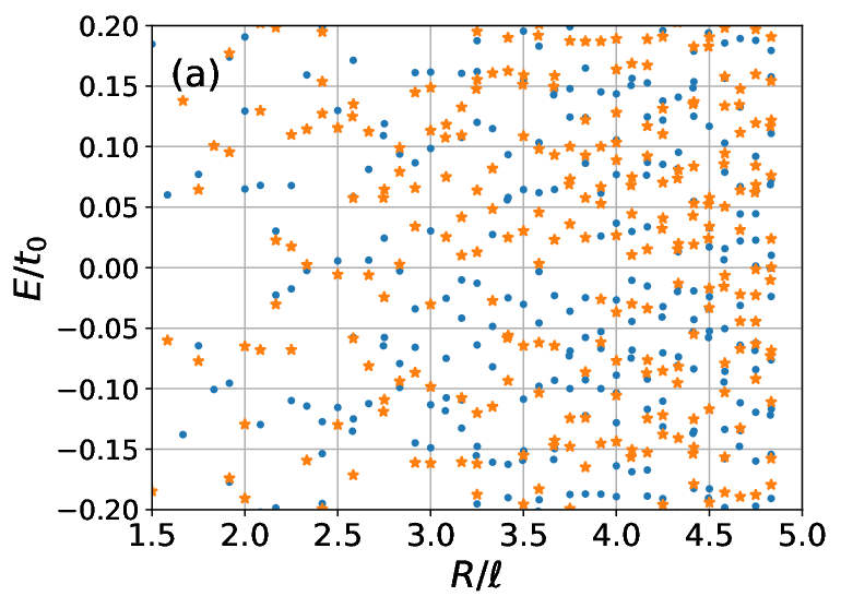
If everywhere within the AA-QD, we have an AA-QD with a “sharp” edge, whose spectrum is shown in Fig. 3(a). Such a termination type introduces strong diffusive scattering into the system due to edge irregularities, see Fig. 1(b). As a result, the energy spectrum is significantly randomized.
Finite on-site potential at the dot’s periphery opens a local gap near the boundary Giovannetti et al. 2007; Gusynin et al. 2007. The gap pushes electrons away from the dot’s boundary, reducing the effect of the diffusive scattering and making the edge effectively “soft”. For numerical calculations, we set
| (31) |
where the parameters and are chosen to be and eV.
| Numerical, | Numerical, | Analytical model, | |
|---|---|---|---|
| geometric | adjusted | ||
| 2.0 | 1.4 | 1.4 | |
| 3.1 | 2.5 | 2.6 | |
| 3.5 | 2.9 | 3.1 | |
| 4.1 | 3.5 | 3.8 |
The spectra for dots with “soft” edges are plotted in Fig. 3 (b). We see similar trends as in our analytical model [compare Fig. 3(b) and Fig. 2]: one can discern layer-symmetric (layer-antisymmetric) states, whose energy increases (decreases) when grows. Moreover, the spectrum demonstrates double degeneracy, similar to the degeneracy in our analytical model. The magic radii sequence can be easily obtained from the results shown in Fig. 3(b). The first four magic radii are shown in Table 1.
Comparing the numerically calculated radii against the results of our analytical model, it is necessary to keep in mind that the geometric radius of an AA-QD with the “soft” edge surpasses the radius of the area accessible to low-energy electrons. Indeed, the potential pushes electrons away from dot periphery, turning the ring into a classically forbidden area. There, a wave function decays as , where is a semiclassical momentum of a Dirac-type quantum particle inside the forbidden ring. Evaluating the integral (it runs from the classical turning point to the position inside the forbidden area), we extract the characteristic length scale over which the wave function decays. Thus, the area accessible for the electrons inside the dot is limited by the radius for our parameters choice. This means that the geometric radius must be reduced by , or, equivalently, by , to account for the inaccessible dot’s periphery. As for the analytical model, it is necessary to remember that the magic sequence is sensitive to the boundary condition parameter . We find that magic radii sequence compares quite well against the (adjusted) magic radii obtained numerically, see Table 1.
For “sharp” termination, the diffusive scattering makes the spectrum irregular, see Fig. 3(a). In this case, the (near) coincidence of the layer-symmetric and layer-antisymmetric eigenenergies for certain values of indicate that this is a magic radius for a specific doping value.
The numerical results confirm the existence of the magic radii sequence in the AA-QD. Moreover, this feature of the dot is very stable with respect to variation of the boundary condition and is a general property that follows from the layer-symmetry of the AA-based systems.
V Discussion
V.1 Magic size of the triangular AA-QD
We would like to stress that the degeneracy enhancement at magic values of is a direct consequence of the peculiar structure of the AA-BLG spectrum, and has no immediate connection to the quantum dot shape. To illustrate this point, we discuss the case of the triangular AA-QD with the edges of the armchair type, see Fig. 4.

Triangular single-layer quantum dots with the armchair edges have been investigated in Ref. Rozhkov and Nori 2010. There, the analytical expression for the single-electron spectrum has been derived [see Eq.(81) of Ref. Rozhkov and Nori 2010]. In terms of our notation it reads , where is the lateral size of the dot, and and are integers.
The dimensionless spectrum of the triangular AA-QD is
| (32) |
where , as above, is the layer-parity eigenvalue. The magic value of is determined by the condition . This generates a sequence of magic sizes (in units of ) parametrized by two integers
| (33) |
Of course, the size being a discrete quantity changing in multiples of cannot exactly satisfy the latter equation. However, due to smallness of relative to , a very accurate tuning can be achieved.
Substituting specific values for and , we calculate , , , , as the first four members of the magic sequence.
V.2 Comparison with other graphene quantum dots
We have seen above that an AA-QD has an interesting property: it demonstrates a sequence of radii at which its ground state experiences an extended degeneracy. This feature persists regardless of the doping and boundary condition at the dot boundary and relates with the specific symmetry of the AA-QD wave functions: the highest occupied state is layer-symmetric () state if is somewhat smaller than the nearest magic value , while, when slightly exceeds , the highest occupied state is layer-antisymmetric (), see Figs. 2 and 3. The system has extra degeneracy at when the highest occupied state changes its layer parity. A quantum dot made from the SLG does not possess this property, neither does a dot from the AB-BLG. Thus, the existence of the sequence of the magic radii is a unique feature of the AA-QD.
To illustrate this, let us consider the QD cut out from the SLG (SLG-QD). The spectrum of the SLG-QD can be obtained directly from the results for the AA-QD by assigning . In so doing, we derive equation for the energy spectrum in the form
| (34) |
Thus, the energy spectrum of the SLG-QD scales as , which is a set of hyperbolas with no magic radii (that is, no crossing points and extra degeneracy).

For the case of the AB-QD we obtain a similar result. We observe that the operator does not commute with the Hamiltonian of the AB-BLG: to map one layer of the AB-BLG to another we should not only apply a mirror transformation but also perform a shift of the layers Rozhkov et al. 2016. As result, there is no quantum number responsible for the extra degeneracy. A direct calculations show that the eigenenergies of the AB-QD scale as . Numerically calculated low-energy spectra for AB-QD of various radii are plotted in Fig. 5. To soften the effects of the edge irregularities, the on-site potential of Eq. (31) is introduced in both layers. The data clearly indicates that for an undoped AB-QD there is no magic radius, and finite gap separates the ground state and excited states.
V.3 Magic radii and magic twist angles
Discovery of an unusual superconductivity Cao et al. 2018a and Mott transitions Cao et al. 2018b in the tBLG with the magic twist angle excited keen interest and a flurry of works on this system. However, a theoretical treatment of the problem encounters a significant difficulty. Indeed, the first magic twist angle is about . Therefore, the tBLG superlattice unit cell includes several thousands of carbon atoms in non-equivalent positions. The analytical or numerical study of such a system is a highly non-trivial task. We believe that our results may be important for the theory of the twisted bilayer graphene as they can form a basis for development a simple model of the tBLG with magic twist angles.
To make the connection between the AA-QD and the tBLG, let us consider the following line of reasoning. The tBLG can be treated as a periodic structure of AA and AB regions surrounded by areas with some intermediate stacking types. It is known that the low-energy electron states are localized within the AA regions of the tBLG móire cell Rozhkov et al. 2016; Lopes dos Santos et al. 2012; San-Jose et al. 2012; Yin et al. 2015. Consequently, one can foresee that the corresponding wave functions may be described by the formalism developed in this paper. For large-size móire cell at , it is also natural to expect, that boundary conditions for a wave function in the AA region does not give rise to either diffusive or inter-valley scattering. Then, we can use Eqs. (11) and (12) with boundary condition (15) to describe the low-energy states in the tBLG. The hybridization between móire cells broadens the AA-localized single-electron states into eight coherent bands (one band per Dirac cone valley, per spin, per layer parity). These bands are separated from other electron states by a gap of the order 0.1 eV. This establishes the desired mapping between the spectrum of the “magic" AA-QD and the low-energy band structure of the tBLG at the magic twist angles Lopes dos Santos et al. 2012; San-Jose et al. 2012; Sboychakov et al. 2015; Utama et al. 2021. When the system departs from a “magic state” (either magic radius or magic twist angle), the band arrangement drastically changes: the degeneracy disappear and the bandwidth increases by order of magnitude. This fact has also a simple explanation within the proposed framework. Indeed, we can expect that the band width is the smallest when the bands degeneracy is maximal. This happens when the AA region size is close to a magic radius. Since is proportional to , the latter condition can be used to link the magic angle and the magic radius of the AA region. A characteristic móire size can be estimated as and for the first magic angle we have . As for , it is naturally smaller than . It can be estimated as follows. It is known Trambly de Laissardière et al. 2010; Anđelković et al. 2018 that at small twist angles the supercell of the twisted bilayer graphene can be considered as consisting of regions with AA, AB, and BA stackings of the same area. The area of the superlattice cell is . Thus, we have the estimate: . According to the results shown in Fig. 3, depending on the boundary conditions, for the first magic radius we have , which is consistent with our estimate for for the tBLG at the first magic angle.
In this paper we focus on the peculiarities of the single-electron spectrum of the AA-QD. The next step in the study of this structure is to take into account the electron-electron interaction and to analyze many-body effects. We believe that the many-body physics of the AA-QD is as rich as the physics of AA-BLG. Moreover, the features of the single-electron spectrum of the AA-QD near the magic radii give rise to arising interesting collective phenomena. We also believe that the study of these phenomena allows us to understand some important effects in the magic angle tBLG.
VI Conclusions
In conclusions, we have studied the electronic properties of a circular quantum dot made from AA bilayer graphene. We observe a discrete set of “magic” radii, where the ground state is degenerate with respect to the layer parity. There is an analogy between “magic angles" of the twisted bilayer graphene and “magic radii" of the AA bilayer graphene quantum dot. The existence of “magic radii” is unique for the AA structures and is related to the layer-symmetry of the AA graphene bilayer. The analogy between “magic angles" and “magic radii" can be helpful for the description of the electronic properties of the twisted bilayer graphene.
Acknowledgments
The numerical calculations and data analysis were funded by the RSF grant No. 22-22-00464, https://rscf.ru/en/project/22-22-00464/.
References
- Rozhkov et al. (2016) A. V. Rozhkov, A. O. Sboychakov, A. L. Rakhmanov, and F. Nori, “Electronic properties of graphene-based bilayer systems,” Phys. Reports 648, 1 (2016).
- Roy et al. (1998) H.-V. Roy, C. Kallinger, and K. Sattler, “Study of single and multiple foldings of graphitic sheets,” Surf. Sci. 407, 1 (1998).
- Lee et al. (2008) J.-K. Lee, S.-C. Lee, J.-P. Ahn, S.-C. Kim, J. I. B. Wilson, and P. John, “The growth of AA graphite on (111) diamond,” J. Chem. Phys. 129, 234709 (2008).
- Liu et al. (2009) Z. Liu, K. Suenaga, P. J. F. Harris, and S. Iijima, “Open and Closed Edges of Graphene Layers,” Phys. Rev. Lett. 102, 015501 (2009).
- Borysiuk et al. (2011) J. Borysiuk, J. Soltys, and J. Piechota, “Stacking sequence dependence of graphene layers on SiC (0001) - Experimental and theoretical investigation,” J. Appl. Phys. 109, 093523 (2011).
- Charlier et al. (1991) J.-C. Charlier, J.-P. Michenaud, X. Gonze, and J.-P. Vigneron, “Tight-binding model for the electronic properties of simple hexagonal graphite,” Phys. Rev. B 44, 13237 (1991).
- Charlier et al. (1992) J.-C. Charlier, J.-P. Michenaud, and X. Gonze, “First-principles study of the electronic properties of simple hexagonal graphite,” Phys. Rev. B 46, 4531 (1992).
- Charlier et al. (1994) J.-C. Charlier, X. Gonze, and J.-P. Michenaud, “First-principles study of the stacking effect on the electronic properties of graphite(s),” Carbon 32, 289 (1994).
- Rakhmanov et al. (2012) A. L. Rakhmanov, A. V. Rozhkov, A. O. Sboychakov, and F. Nori, “Instabilities of the -Stacked Graphene Bilayer,” Phys. Rev. Lett. 109, 206801 (2012).
- Sboychakov et al. (2013a) A. O. Sboychakov, A. L. Rakhmanov, A. V. Rozhkov, and F. Nori, “Metal-insulator transition and phase separation in doped AA-stacked graphene bilayer,” Phys. Rev. B 87, 121401 (2013a).
- Sboychakov et al. (2013b) A. O. Sboychakov, A. V. Rozhkov, A. L. Rakhmanov, and F. Nori, “Antiferromagnetic states and phase separation in doped AA-stacked graphene bilayers,” Phys. Rev. B 88, 045409 (2013b).
- Akzyanov et al. (2014) R. S. Akzyanov, A. O. Sboychakov, A. V. Rozhkov, A. L. Rakhmanov, and F. Nori, “AA-stacked bilayer graphene in an applied electric field: Tunable antiferromagnetism and coexisting exciton order parameter,” Phys. Rev. B 90, 155415 (2014).
- Mosoyan et al. (2018) K. S. Mosoyan, A. V. Rozhkov, A. O. Sboychakov, and A. L. Rakhmanov, “Spin-density wave state in simple hexagonal graphite,” Phys. Rev. B 97, 075131 (2018).
- Brey and Fertig (2013) L. Brey and H. A. Fertig, “Gapped phase in -stacked bilayer graphene,” Phys. Rev. B 87, 115411 (2013).
- Sboychakov et al. (2021) A. O. Sboychakov, A. L. Rakhmanov, A. V. Rozhkov, and F. Nori, “Bilayer graphene can become a fractional metal,” Phys. Rev. B 103, L081106 (2021).
- Chiu et al. (2010) C. W. Chiu, S. H. Lee, S. C. Chen, F. L. Shyu, and M. F. Lin, “Absorption spectra of AA-stacked graphite,” New J. Phys. 12, 083060 (2010).
- Alam et al. (2011) M. S. Alam, J. Lin, and M. Saito, “First-Principles Calculation of the Interlayer Distance of the Two-Layer Graphene,” Jpn. J. Appl. Phys. 50, 080213 (2011).
- Chang (2012) C. P. Chang, “Analytic model of energy spectrum and absorption spectra of bilayer graphene,” J. Appl. Phys. 111, 103714 (2012).
- Apinyan and Kopeć (2021) V. Apinyan and T. K. Kopeć, “Antiferromagnetic ordering and excitonic pairing in AA-stacked bilayer graphene,” Phys. Rev. B 104, 075426 (2021).
- Rozhkov et al. (2017) A. V. Rozhkov, A. L. Rakhmanov, A. O. Sboychakov, K. I. Kugel, and F. Nori, “Spin-Valley Half-Metal as a Prospective Material for Spin Valleytronics,” Phys. Rev. Lett. 119, 107601 (2017).
- Akhmerov and Beenakker (2008) A. R. Akhmerov and C. W. J. Beenakker, “Boundary conditions for Dirac fermions on a terminated honeycomb lattice,” Phys. Rev. B 77, 085423 (2008).
- Sanderson et al. (2013) M. Sanderson, Y. S. Ang, and C. Zhang, “Klein tunneling and cone transport in AA-stacked bilayer graphene,” Phys. Rev. B 88, 245404 (2013).
- Giovannetti et al. (2007) G. Giovannetti, P. A. Khomyakov, G. Brocks, P. J. Kelly, and J. van den Brink, “Substrate-induced band gap in graphene on hexagonal boron nitride: Ab initio density functional calculations,” Phys. Rev. B 76, 073103 (2007).
- Gusynin et al. (2007) V. Gusynin, S. Sharapov, and J. Carbotte, “AC conductivity of graphene: from tight-binding model to 2+ 1-dimensional quantum electrodynamics,” International Journal of Modern Physics B 21, 4611 (2007).
- Rozhkov and Nori (2010) A. V. Rozhkov and F. Nori, “Exact wave functions for an electron on a graphene triangular quantum dot,” Phys. Rev. B 81, 155401 (2010).
- Cao et al. (2018a) Y. Cao, V. Fatemi, S. Fang, K. Watanabe, T. Taniguchi, E. Kaxiras, and P. Jarillo-Herrero, “Unconventional superconductivity in magic-angle graphene superlattices,” Nature 556, 43 (2018a).
- Cao et al. (2018b) Y. Cao, V. Fatemi, A. Demir, S. Fang, S. L. Tomarken, J. Y. Luo, J. D. Sanchez-Yamagishi, K. Watanabe, T. Taniguchi, E. Kaxiras, et al., “Correlated insulator behaviour at half-filling in magic-angle graphene superlattices,” Nature 556, 80 (2018b).
- Lopes dos Santos et al. (2012) J. M. B. Lopes dos Santos, N. M. R. Peres, and A. H. Castro Neto, “Continuum model of the twisted graphene bilayer,” Phys. Rev. B 86, 155449 (2012).
- San-Jose et al. (2012) P. San-Jose, J. González, and F. Guinea, “Non-Abelian Gauge Potentials in Graphene Bilayers,” Phys. Rev. Lett. 108, 216802 (2012).
- Yin et al. (2015) L.-J. Yin, J.-B. Qiao, W.-J. Zuo, W.-T. Li, and L. He, “Experimental evidence for non-Abelian gauge potentials in twisted graphene bilayers,” Phys. Rev. B 92, 081406 (2015).
- Sboychakov et al. (2015) A. O. Sboychakov, A. L. Rakhmanov, A. V. Rozhkov, and F. Nori, “Electronic spectrum of twisted bilayer graphene,” Phys. Rev. B 92, 075402 (2015).
- Utama et al. (2021) M. I. B. Utama, R. J. Koch, K. Lee, N. Leconte, H. Li, S. Zhao, L. Jiang, J. Zhu, K. Watanabe, T. Taniguchi, et al., “Visualization of the flat electronic band in twisted bilayer graphene near the magic angle twist,” Nat. Phys. 17, 184 (2021).
- Trambly de Laissardière et al. (2010) G. Trambly de Laissardière, D. Mayou, and L. Magaud, “Localization of Dirac Electrons in Rotated Graphene Bilayers,” Nano Lett. 10, 804 (2010).
- Anđelković et al. (2018) M. Anđelković, L. Covaci, and F. M. Peeters, “DC conductivity of twisted bilayer graphene: Angle-dependent transport properties and effects of disorder,” Phys. Rev. Materials 2, 034004 (2018).