Theory-agnostic Reconstruction of Potential and Couplings from Quasi-Normal Modes
Abstract
In this work, we use a parametrized theory-agnostic approach that connects the observation of black hole quasi-normal modes with the underlying perturbation equations, with the goal of reconstructing the potential and the coupling functions appearing in the latter. The fundamental quasi-normal mode frequency and its first two overtones are modeled through a second order expansion in the deviations from general relativity, which are assumed to be small but otherwise generic. By using a principal component analysis, we demonstrate that percent-level measurements of the fundamental mode and its overtones can be used to constrain the effective potential of tensor perturbations and the coupling functions between tensor modes and ones of different helicity, without assuming an underlying theory. We also apply our theory-agnostic reconstruction framework to analyze simulated quasi-normal mode data produced within specific theories extending general relativity, such as Chern-Simons gravity.
I Introduction
After the first detection of the binary black hole (BH) merger GW150914 Abbott et al. 2016a, the relentless experimental efforts conducted at the LIGO/Virgo interferometers have resulted in the detection of almost 100 more compact binary mergers Abbott et al. 2019a; Abbott et al. 2021a; Abbott et al. 2021b. These detections will become more numerous as the sensitivity of these interferometers will increase and additional instruments will join the network (as recently done by KAGRA). Besides a few exceptions involving neutron stars Abbott et al. 2017; Abbott et al. 2021c, most of these events are binary BH mergers. On top of the astrophysical and cosmological implications that can be drawn from this growing experimental sample, there is also a significant interest in using it to test the validity of general relativity (GR) in the strong and dynamical regime Abbott et al. 2016b; Abbott et al. 2019b; Abbott et al. 2021d; Abbott et al. 2021e.
Many ongoing works aim to use the ringdown regime of binary BH mergers to conduct precision tests of the no-hair theorems’ hypotheses (“BH spectroscopy”). By measuring multiple quasi-normal modes (QNMs), quantitative experimental tests of the linearized perturbation equations of the Schwarzschild/Kerr space-time will become possible. Nevertheless, although perturbative calculations can be used to define the QNM spectrum as an eigenvalue problem, numerical relativity simulations are still needed to understand the range of validity of the perturbative regime, which is a problem still under development Isi et al. 2019; Giesler et al. 2019; Jiménez Forteza et al. 2020; Cook 2020.
In recent years, there have been several studies aiming to extract QNMs from real gravitational wave measurements Abbott et al. 2016b; Abbott et al. 2019b; Abbott et al. 2021d; Abbott et al. 2021e; Isi et al. 2019; Giesler et al. 2019; Jiménez Forteza et al. 2020; Cook 2020; Ghosh et al. 2021; Cotesta et al. 2022. The LIGO-Virgo collaboration reported that the and mode has been clearly extracted from GW150914 Abbott et al. 2016b, and follow up works Isi et al. 2019; Giesler et al. 2019 claim evidence also for the and overtones, although with much greater uncertainty and a robustness still under debate Cotesta et al. 2022; Isi and Farr 2022. Under certain assumptions, it is possible to combine measurements from different GW events Ghosh et al. 2021, providing more stringent bounds on possible deviations of the fundamental mode frequency from GR. The prospects to measure the mode have also been studied in Ref. Cabero et al. 2020.
Tests of GR, currently limited by the signal-to-noise ratio of the post-merger signal, will become easier with future, more sensitive detectors Berti et al. 2016, although the increasing number of free parameters needed to quantify deviations from GR can be problematic Bustillo et al. 2021. A task even more difficult than detecting a deviation from GR in the QNMs (if any) will be the extraction of information about the underlying theory or background metric. Although parametrized frameworks to capture modifications as function of BH mass and spin have been developed Maselli et al. 2020; Carullo 2021, they cannot be readily used to learn about the fundamental structure of the equations governing the perturbations, nor about the underlying theory itself.
In general, a discrepancy with GR would manifest both in deviations of the background BH metric from the Schwarzschild/Kerr solution Schwarzschild 1916; Kerr 1963, and in deviations from the linearized perturbation equations of GR (i.e. the Regge-Wheeler/Zerilli equations for Schwarzschild Regge and Wheeler 1957; Zerilli 1970 or the Teukolsky equation for Kerr Teukolsky 1973), see Ref. Barausse and Sotiriou 2008. Under the assumption that corrections to GR are “small”, the deviations can be parametrized in the perturbation equations defining the QNM spectrum via a fixed set of theory-agnostic coefficients Cardoso et al. 2019; McManus et al. 2019. This framework can then be used to attempt to solve an “inverse problem”, i.e. to determine the form of the perturbation equations from a given set of QNM observations.
In this work, we tackle this inverse problem in the non-rotating (spherical) case. More specifically, we focus on the possibility that the gravitational perturbations of different parity (axial and polar) may obey potentials deviating from GR and, moreover, that they can couple to a hypothetical scalar degree of freedom. While in GR a scalar degree of freedom is absent, it is a very common feature in many alternative theories of gravity Berti et al. 2015, e.g. dynamical Chern-Simons gravity Alexander and Yunes 2009 or degenerate higher-order scalar-tensor theories (DHOST) theories Langlois et al. 2021.
In order to address the problem, we use and extend the parametrized framework introduced by Ref. Cardoso et al. 2019; McManus et al. 2019 to handle QNM overtones, and produce a “clean” reconstruction by performing a principal component analysis (PCA) Sivia and Skilling 2006; Pieroni and Barausse 2020; Lara et al. 2021. The parametrized framework allows for a quick modeling of QNMs for small deviations from GR, while the PCA reveals the non-degenerate combinations of the parameters that can be extracted from the data. We explicitly demonstrate the capabilities of our framework to constrain injected deviations from GR in the effective potentials and coupling functions, provided that QNMs are known to within percent level.
This work is structured as follows. In Sec. II we review BH perturbation theory and the parametrized framework of Cardoso et al. 2019; McManus et al. 2019; Sec. III covers the details of the numerical and parameter estimation methods. The application and results are discussed in Sec. IV. An overall conclusion is found in Sec. V. Throughout this work, we use units in which .
II Theoretical Framework
The equations describing tensor and scalar perturbations of a non-spinning BH in GR are derived by linearizing respectively the Einstein and the Klein-Gordon equations, on top of a Schwarzschild geometry. These equations would depend in general on time, radius and angular coordinates. An expansion of the perturbation functions in spherical tensor or scalar harmonics eliminates the angular coordinates from the equations and decouples them. A solution to the resultant equation can be either found in the time domain, or, after performing a Fourier transform, in the frequency domain. The axial-parity equation for tensor perturbations is known as Regge-Wheeler equation Regge and Wheeler 1957, whereas the Zerilli equation describes polar-parity tensor perturbations Zerilli 1970. The perturbed Klein-Gordon equation for a scalar field takes a similar form. For useful reviews on the topic we refer the interested reader to Refs. Kokkotas and Schmidt 1999; Nollert 1999; Berti et al. 2009; Pani 2013.
Working in the frequency domain, the system of radial perturbation equations for coupled fields of any helicity (tensor or scalar) around a spherically symmetric and static BH takes the general form
| (1) |
In this equation, is the areal coordinate, (with the areal radius of the event horizon) and is the complex perturbation frequency. For each field, there is an infinite but discrete set of eigenfrequencies , where is the overtone number (characterizing the number of nodes of the radial solution) and its angular momentum number. The diagonal terms of the matrix are the potentials felt by each field, while the non-diagonal ones represent coupling terms between fields. We can thus write
| (2) | ||||
| (3) |
where the matrix is diagonal ( and for ) and represents the GR potentials, while the parameters are assumed to be small and describe a generic deviation from GR. In more detail, the GR potentials for scalar and tensor (axial and polar) modes are given by
| (4) | ||||
| (5) | ||||
| (6) |
where .
One can solve the eigenvalue problem for described by Eq. (1), with ingoing boundary conditions at the event horizon and outgoing ones at infinity. Different methods can be used for this purpose. In this paper, in order to get the coefficients for the fundamental mode and the first two overtones, we employed a continued fraction method Pani 2013; Leaver 1985; Rosa and Dolan 2012, which provides more stable results than other methods, e.g., direct integration. The details are explained in Appendices A-B. Summarizing, the problem reduces to the computation of a complex function for each choice of , and , and the corresponding eigenfrequencies correspond to the zeroes of this function. We denote the frequencies of the unperturbed GR problem, corresponding to , as , and we compute the non-GR frequencies through quadratic order in the coefficients as
| (7) |
where we omitted the indices for readability.11 1 In principle, there would be a quadratic contribution when the parameters depend on the frequency McManus et al. 2019. However, in our analysis we consider the parameters being independent from , therefore, we do not show this term here.
One then needs to compute the coefficients and , which are independent from the specific deviation from GR under scrutiny, which is encoded in the parameters alone. In practice, one can determine the coefficients by Taylor expanding the complex function for small . One can then show that the coefficients and can be computed from a combination of the derivatives of the master function with respect to the frequency and the parameters , evaluated for McManus et al. 2019. We have checked the coefficients against those already computed in Cardoso et al. 2019; McManus et al. 2019 and, despite the different method, they are in very good agreement.
We have extended the computation of the linear and quadratic coefficients, for both one field and two coupled fields, to the first two overtones for . Table 1 shows some of the coefficients for for axial tensor perturbations. It is clear from the table that increasing the overtone number makes the coefficients grow for fixed . To better visualize this behaviour, in Fig. 1 we show the linear and diagonal quadratic coefficients, respectively and , for the axial case, plotting their real and imaginary part. The case with with is not shown in the plot, but follows the same trend.
This behavior directly affects the QNMs, as can be seen in Fig. 2. Here, we choose a fixed value for and compute the modified frequencies with only one component (selected in the range ). We display how the coefficients affect the real and imaginary frequencies, normalized by their GR values. Note that in GR the absolute value of the complex QNM frequencies increases with overtone number, which qualitatively implies that also the coefficients and should increase, if they correspond to a roughly similar change in the QNM spectrum.
This behaviour suggests that higher modes are more sensitive to changes in the potential. We can provide a rough explanation of this with the Wentzel-Kramer-Brillouin (WKB) approximation Schutz and Will 1985; Iyer and Will 1987; Konoplya 2003. This method connects the QNM frequencies to the derivatives of the effective potential with respect to the tortoise coordinate around its maximum . Studying the numerical precision of the WKB approximation implies that the higher the overtone, the more derivatives of the effective potential one has to take into account. While modifications to the potential at its peak are proportional to , its higher derivatives show a different decrease rate for large , affecting the magnitude of the overtones more significantly.


III Principal Component Analysis
In this paper, we assume the observation of a certain number of QNMs, namely the fundamental mode and up to two more overtones . We collectively denote them as the data and we assume that they are measured with error , with the index labeling the different data points and running from to (as we treat the real and imaginary parts of the QNM frequencies independently).
The model that we employ to describe the data is given by Eq. (7). Each QNM frequency predicted by the model is denoted by , where is the vector containing all the parameters .22 2 To avoid cluttering the notation, we refer to the components of as . The index runs from to , being and the values determining the range of basis functions that we consider in Eq. (3). Note that in general the parameters can be complex numbers, representing complex valued contributions from . Although these can in principle arise for specific cases, for example when the potential becomes frequency dependent, we assume from here on that all are real numbers. A generalization to complex potentials is in principle straightforward, but introduces additional degeneracy to the inverse problem, which we will suppress implicitly in the following.
To construct the likelihood of the problem, we assume the QNM measurements to be uncorrelated and described by a Gaussian distribution with variance . If the horizon location of the final BH were known, the likelihood would then be defined by a simple Gaussian distribution, whose logarithm would be proportional to
| (8) |
However, in general is not known, and it is therefore more robust to generalize Eq. (8) to take this into account.
In GR, , and one could therefore try to estimate it from the measurement of the individual BH masses during the inspiral Barausse et al. 2012. However, the errors on the masses would propagate into the estimate of . Moreover, beyond GR effects would generally make be different from . To model these uncertainties, we assume , where is the GR expectation for , and the deviation from it (due to errors in the measurement of the individual masses and to deviations from GR). By making the simplifying assumption that is a Gaussian variable, we can write the likelihood as
| (9) |
where
| (10) |
Here, and is the relative error on . The term multiplying arises from the scaling of the observed frequencies with the BH horizon radius .
To get rid of we can then marginalize over it, obtaining the likelihood
| (11) |
with
| (12) | ||||
| (13) |
In the following, we assume . This choice is based on the underlying assumptions that the estimate on the final mass from the inspiral signal assuming GR will have small errors and that modifications to GR are small. This ensures that the location of the horizon will be approximated by .
With flat priors, the best-fit parameters (which we denote by ) can be estimated from the maximum of the likelihood Eq. (11). We compute them by using the L-BFGS-B optimization method provided in the open source software package SciPy for Python Virtanen et al. 2020. We start from an initial guess for the parameters given by GR plus small random noise. To remain in the regime where the quadratic expansion of Eq. (7) can be trusted, we bound the parameter search intervals for the parameters to be of order unit. Furthermore, by performing a quadratic expansion of the the log-likelihood near the maximum, one can obtain information on the errors of the best-fit parameters. In more detail, the Hessian matrix evaluated at ,
| (14) |
is the inverse of the covariance matrix of the parameters. [Note the minus sign in Eq. (14) to make the Hessian positive definite.]
In order to further clean the reconstruction of the potentials encoded in the best-fit parameters, we employ a technique called PCA Sivia and Skilling 2006; Pieroni and Barausse 2020; Lara et al. 2021, which we use to “denoise” the reconstruction of . The PCA allows one to find the linear combinations of the parameters that are best determined by a given set of QNMs. This can be done by computing the eigenvalues and eigenvectors of the Hessian Eq. (14). In this new basis, the eigenfunctions are orthogonal and their coefficients follow from projecting the best-fit parameters onto the eigenvectors:
| (15) |
The errors on the coefficients are then given by the square root of the inverse of the eigenvalues, .
The “denoising” of the PCA is then achieved by selecting only the components that contribute significantly to the data. A possible criterion used e.g. in Ref. Pieroni and Barausse 2020 consists of retaining only components for which
| (16) |
where allows only for eigenvectors that are not consistent with noise at 1-. This will select a set of eigenvectors. The PCA reconstructed parameters are finally obtained as
| (17) |
In appendix C, we will discuss how different selection criteria affect the reconstruction.
With one can now compute the reconstruction of the potential as
| (18) |
while the errors on the potential can be obtained by summing in quadrature the errors on the retained coefficients , which are Gaussian and uncorrelated
| (19) |
IV Application and Results
In the following, we consider various simulated QNMs as mock data, evaluated with full numerical calculations using the continued fraction method. As discussed in the Introduction, the and corresponding QNM frequencies are in principle within reach of current and future detectors. Hence, for the purposes of our reconstruction, a combined measurement of three frequencies simultaneously will be our optimistic assumption, while only one detected frequency our pessimistic assumption. For the sake of clarity, we have decided to focus in this section on results with constant relative errors, i.e. we assume that all frequencies are measured within a error, unless stated otherwise. For better visualization of the injected and reconstructed potentials and coupling functions, we also introduce the compactified coordinate
| (20) |
IV.1 Reconstructing Potentials
As a first example, we apply our framework to modifications in the axial potential only. The assumed injections are of the form for , and we assume no couplings to additional fields. In the model given by Eq. (3), we also truncate the series at . The 2- PCA reconstruction region is shown in Fig. 3, where different colors correspond to different number of observed QNMs. Since GR corresponds to , the injection can be clearly identified by the PCA and GR is excluded. This is already possible with knowledge of the fundamental mode alone, although the injection cannot be correctly identified in this case. It is evident that the inclusion of more QNMs significantly improves the reconstruction of the potential. It is also worth noticing that although QNMs are very sensitive to the light ring region Ferrari and Mashhoon 1984; Schutz and Will 1985 (here around ), our PCA framework can clearly constrain the injection even far from the BH, although with larger uncertainties. Although not shown here, the results for polar tensor fields and the scalar ones are quantitatively very similar.

IV.2 Reconstructing Coupling Functions
As a next application, we consider the presence of a coupling function to a scalar field via and . We assume injections only to originate from the two coupling functions, for which we assume for . In principle, there can also be a contribution from , but we focus here on a case with purely GR potentials. For the PCA reconstruction, we let only the parameters of the coupling functions free to vary (also for ). The results for this case are shown in Fig. 4 and demonstrate that the fundamental mode alone is already enough to identify a significant non-GR contribution.

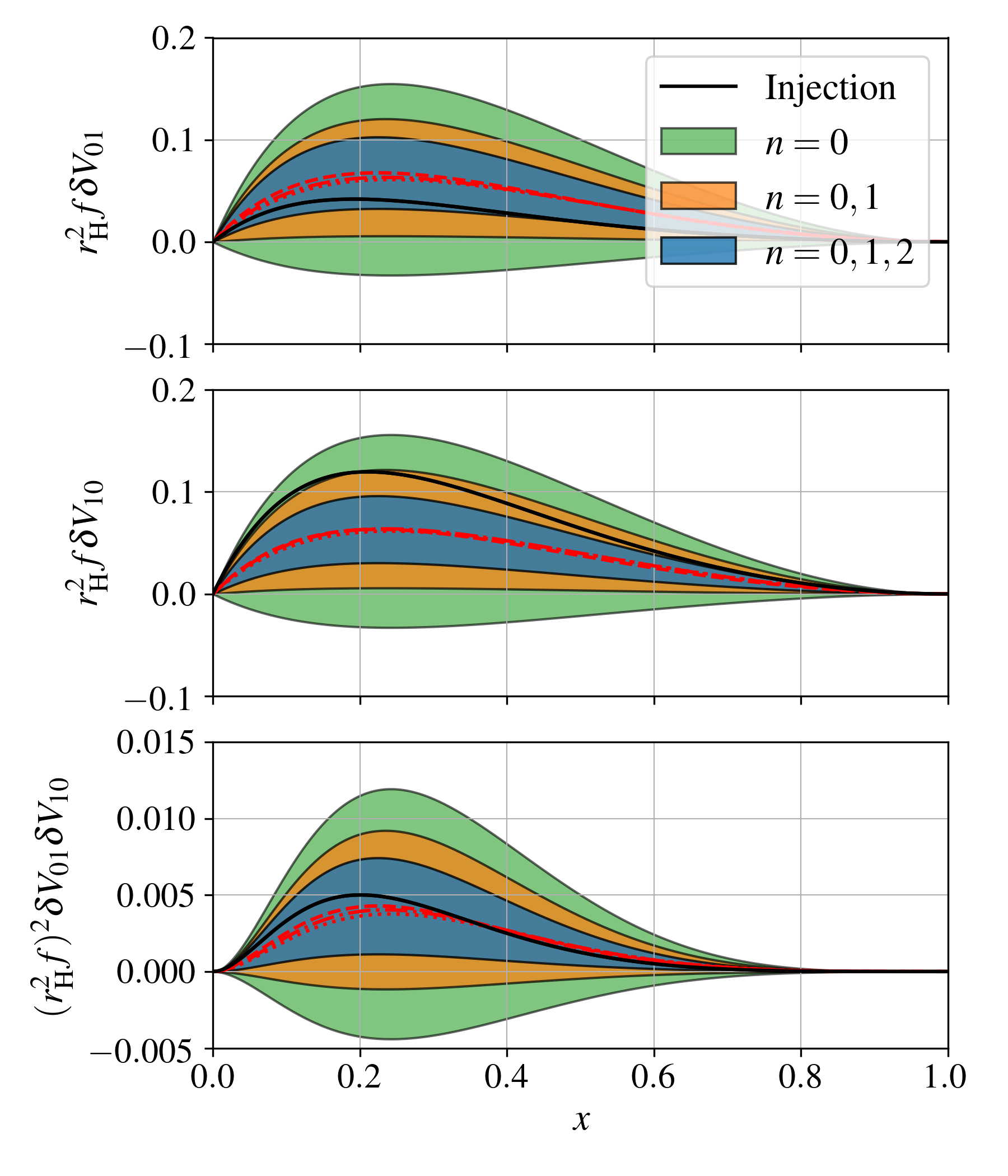
The reconstruction of the coupling functions, however, can suffer from degeneracies when the injection is less trivial than in this first example. Let us then consider the injection given in Table 2, where all the coefficients have different values. In the top and middle panels of Fig. 5, we show the injected coupling functions and their reconstruction when both and are varied. As can be seen, the reconstruction – obtained by assuming the same free parameters in the model of Eq. (3) as in the previous example – is suboptimal. However, if one looks at the product of the coupling functions (bottom panel) the reconstruction improves significantly. Moreover, it is worth noticing that in this example GR would be ruled out only with the measurement of three modes.
This degeneracy can be easily explained in two special limiting cases. The first is when both coupling functions have exactly one non-zero contribution , while all the others are zero. The second case is when all the contributions for the couplings have the same magnitude—e.g. the one considered for Fig. 4. We denote these magnitudes by and . With a simple field redefinition, one can show that the QNMs in both cases are equivalent to those obtained by replacing and with the same coefficient , given by
| (21) |
From this result, one can infer that the reconstruction of the product of the coupling functions in these special cases must be invariant under the choice of injected parameters, for a fixed choice of . In the most general case, we found out that numerically evaluated spectra are still degenerate upon exchange and . Even if we were not able to prove it formally, this fact strongly suggests that the product of the couplings is the best choice to reconstruct in any case.
IV.3 Dynamical Chern-Simons Gravity
Finally, we consider the case of a specific theory: dynamical Chern-Simons (dCS) gravity Alexander and Yunes 2009. Here, the equations governing the perturbations around non-rotating BHs, which coincide with the Schwarzschild BH Yunes and Stein 2011, can be easily derived Cardoso and Gualtieri 2009; Molina et al. 2010. While the polar equation remains unchanged, the axial and scalar equations are coupled to each other, but the potentials are the same as in GR. As demonstrated in Ref. McManus et al. 2019, the axial QNMs are well approximated by
| (22) |
where depends on the theory’s coupling constant. Note that the latter can also be constrained by gravitational wave observations of the inspiral and mergers Stein and Yagi 2014; Okounkova et al. 2019.
Since we already demonstrated the reconstruction of two independent coupling functions and the product of coupling functions, we now assume that the coupling functions are symmetric, as indeed is the case for dCS. This time, we consider contributions up to in the model of Eq. (3). Our findings for are shown in Fig. 6. Since we assume in this application, we only show . It can be clearly seen that our framework is capable of reconstructing the coupling functions and exclude GR. Moreover, the reconstruction agrees very well with the injection in the region close to the BH, although the agreement degrades further out.

IV.4 Discussion
In all the cases considered above, we have focused on small modifications to the potentials and coupling functions of the scalar, axial and polar fields. As pointed out in Ref. McManus et al. 2019, corrections to the QNM spectrum from the coupling functions enter at quadratic order in the deviations from GR, unless spectra are degenerate. Since quadratic corrections to the QNM spectrum also come from the individual potentials, it is in general very difficult to disentangle the two if they are allowed to vary at the same time. Indeed, we have tried to vary the potential and coupling functions at the same time, but the problem is very degenerate and sensitive to the initial guess of our root finder. This most likely happens as a result of possible multi-modalities in the likelihood/posteriors, calling for a more systematic approach (via e.g. Markov Chain Monte Carlo or nested sampling). We stress, however, that once the global maximum of the posteriors has been located, our PCA method can be applied in the vicinity of the maximum to yield a denoised reconstruction.
Another point that can have an impact on the reconstruction of the potentials is the precision with which the QNMs are known. In the analysis conducted so far, we showed how the reconstruction of the potentials improves when multiple QNMs are provided. However, in that application we assumed optimistic errors on measured frequencies. We now compare the reconstruction of the potential in section IV.1 with one that assumes larger uncertainties for the overtones. In more detail, we now assume that the QNMs are known with relative errors, respectively, while the other assumptions are unchanged. The resulting reconstruction is shown in Fig. 7. By comparing with Fig. 3, it is clear that the reconstruction still approximates well the injection, although the improvement allowed by including the second overtone is now marginal. Nevertheless, one can still confirm a non-GR modification of the potential at high significance.
One may ask how the picture changes if instead of providing multiple overtones for the same , one provides the modes for multiple , see e.g. Gossan et al. 2012. In the current parametrization framework each potential is treated independently because each set of deviations implicitly depends on . This implies one cannot easily combine the QNMs to obtain a better reconstruction. An alternative approach could be to provide a parametrized BH metric and assume a certain structure of the perturbation equations, as done in Ref. Völkel and Barausse 2020. Here one could combine QNMs of different to constrain the same (metric) parameters.
Finally, the reconstruction depends mildly also on the PCA criteria used to select what components are retained in the reconstruction. We discuss this in detail in Appendix C.

V Conclusions
In this work, we have tackled the ‘inverse problem’ of reconstructing the potential of the gravitational perturbations on a spherically symmetric static background from a set of simulated observations of QNMs. We consider both the case of tensorial perturbations only, and that of coupled tensorial and scalar gravitons. In the latter case, we attempt to reconstruct also the coupling functions between the two helicities. Our approach parametrizes the potential and coupling functions in a theory independent way introduced in Refs. Cardoso et al. 2019; McManus et al. 2019, which we generalized to the overtones. In this approach, the only assumption is that the deviations of the gravitational theory from GR are small, and the QNM frequencies are computed through quadratic order in these deviations. Since the problem of reconstructing the potentials and coupling functions in a theory independent formalism is intrinsically degenerate, we employ a PCA to ‘denoise’ the reconstruction. The PCA technique achieves by identifying the ‘modes’ or ‘features’ of the potentials and coupling functions that are best constrained by the data.
Unlike the perturbation potential, which modifies the QNMs already at linear order in the deviations from GR, the presence of couplings between scalar and tensor modes affects the QNM spectrum only at quadratic order. This makes it more difficult to reconstruct coupling functions. Nevertheless, we have shown that given QNM frequency measurements at percent level or better, one can successfully reconstruct at least suitable combinations (products) of the coupling functions. In general, in most of the cases that we considered, our PCA framework allows for the extraction of two to three features, especially if QNM overtones are measured.
In an earlier work, some of us performed a similar analysis of the inverse problem using Bayesian techniques and higher order WKB theory for the computation of QNMs Völkel and Barausse 2020. The latter allowed us to go beyond small modifications from GR, but did not include couplings between modes of different helicity. That work also managed to account for non-trivial correlations between possible modifications of the background space-time and the perturbation equations. We plan to perform a similar reconstruction of the space-time metric (but allowing also the potentials and coupling functions to vary) in future extensions of this paper. This would also open the way to combining information on the background BH geometry from QNM observations with related information from electromagnetic probes, such as X-rays spectra Bambi et al. 2017; Tripathi et al. 2019 and shadow measurements by the Event Horizon Telescope Akiyama et al. 2019a; Akiyama et al. 2019b. Indeed, the latter have been the object of several recent studies to constrain possible deviations of the BH geometry from GR, e.g. Psaltis et al. 2020; Völkel et al. 2021; Kocherlakota et al. 2021; Nampalliwar and K 2021; Kocherlakota and Rezzolla 2022; Lara et al. 2021.
Future developments of our formalism will also include the use of real ringdown data, as well as an extension to the case of rotating BHs. The latter is particularly challenging because even theory specific calculations of QNMs in rotating background are currently limited to the slow rotation approximation Cano et al. 2020; Pierini and Gualtieri 2021; Wagle et al. 2021. Moreover, a different parametrization of the potentials and coupling functions may allow for describing near-horizon deviations from GR Cardoso et al. 2016; Cardoso and Pani 2017, or the presence of matter sources far from the BH Barausse et al. 2014; Cheung et al. 2021. While the deviations produced in the QNM spectrum can be sizeable in these cases, the time-domain ringdown signal is less significantly affected Barausse et al. 2014; Nollert 1996; Nollert and Price 1999; Jaramillo et al. 2021. Therefore, our formalism could be applicable in the time domain.
Acknowledgements.
We would like to thank Emanuele Berti, Andrea Maselli, Ryan McManus and Guillermo Lara for useful discussions. We acknowledge financial support provided under the European Union’s H2020 ERC Consolidator Grant “GRavity from Astrophysical to Microscopic Scales” grant agreement no. GRAMS-815673. This work was supported by the EU Horizon 2020 Research and Innovation Programme under the Marie Sklodowska-Curie Grant Agreement No. 101007855.References
- Abbott et al. (2016a) B. P. Abbott et al. (LIGO Scientific, Virgo), Phys. Rev. Lett. 116, 061102 (2016a), arXiv:1602.03837 [gr-qc] .
- Abbott et al. (2019a) B. P. Abbott et al. (LIGO Scientific, Virgo), Phys. Rev. X 9, 031040 (2019a), arXiv:1811.12907 [astro-ph.HE] .
- Abbott et al. (2021a) R. Abbott et al. (LIGO Scientific, Virgo), Phys. Rev. X 11, 021053 (2021a), arXiv:2010.14527 [gr-qc] .
- Abbott et al. (2021b) R. Abbott et al. (LIGO Scientific, VIRGO, KAGRA), (2021b), arXiv:2111.03606 [gr-qc] .
- Abbott et al. (2017) B. P. Abbott et al. (LIGO Scientific, Virgo), Phys. Rev. Lett. 119, 141101 (2017), arXiv:1709.09660 [gr-qc] .
- Abbott et al. (2021c) R. Abbott et al. (LIGO Scientific, KAGRA, VIRGO), Astrophys. J. Lett. 915, L5 (2021c), arXiv:2106.15163 [astro-ph.HE] .
- Abbott et al. (2016b) B. P. Abbott et al. (LIGO Scientific, Virgo), Phys. Rev. Lett. 116, 221101 (2016b), [Erratum: Phys.Rev.Lett. 121, 129902 (2018)], arXiv:1602.03841 [gr-qc] .
- Abbott et al. (2019b) B. P. Abbott et al. (LIGO Scientific, Virgo), Phys. Rev. D 100, 104036 (2019b), arXiv:1903.04467 [gr-qc] .
- Abbott et al. (2021d) R. Abbott et al. (LIGO Scientific, Virgo), Phys. Rev. D 103, 122002 (2021d), arXiv:2010.14529 [gr-qc] .
- Abbott et al. (2021e) R. Abbott et al. (LIGO Scientific, VIRGO, KAGRA), (2021e), arXiv:2112.06861 [gr-qc] .
- Isi et al. (2019) M. Isi, M. Giesler, W. M. Farr, M. A. Scheel, and S. A. Teukolsky, Phys. Rev. Lett. 123, 111102 (2019), arXiv:1905.00869 [gr-qc] .
- Giesler et al. (2019) M. Giesler, M. Isi, M. A. Scheel, and S. Teukolsky, Phys. Rev. X 9, 041060 (2019), arXiv:1903.08284 [gr-qc] .
- Jiménez Forteza et al. (2020) X. Jiménez Forteza, S. Bhagwat, P. Pani, and V. Ferrari, Phys. Rev. D 102, 044053 (2020), arXiv:2005.03260 [gr-qc] .
- Cook (2020) G. B. Cook, Phys. Rev. D 102, 024027 (2020), arXiv:2004.08347 [gr-qc] .
- Ghosh et al. (2021) A. Ghosh, R. Brito, and A. Buonanno, Phys. Rev. D 103, 124041 (2021), arXiv:2104.01906 [gr-qc] .
- Cotesta et al. (2022) R. Cotesta, G. Carullo, E. Berti, and V. Cardoso, (2022), arXiv:2201.00822 [gr-qc] .
- Isi and Farr (2022) M. Isi and W. M. Farr, (2022), arXiv:2202.02941 [gr-qc] .
- Cabero et al. (2020) M. Cabero, J. Westerweck, C. D. Capano, S. Kumar, A. B. Nielsen, and B. Krishnan, Phys. Rev. D 101, 064044 (2020), arXiv:1911.01361 [gr-qc] .
- Berti et al. (2016) E. Berti, A. Sesana, E. Barausse, V. Cardoso, and K. Belczynski, Phys. Rev. Lett. 117, 101102 (2016), arXiv:1605.09286 [gr-qc] .
- Bustillo et al. (2021) J. C. Bustillo, P. D. Lasky, and E. Thrane, Phys. Rev. D 103, 024041 (2021), arXiv:2010.01857 [gr-qc] .
- Maselli et al. (2020) A. Maselli, P. Pani, L. Gualtieri, and E. Berti, Phys. Rev. D 101, 024043 (2020), arXiv:1910.12893 [gr-qc] .
- Carullo (2021) G. Carullo, Phys. Rev. D 103, 124043 (2021), arXiv:2102.05939 [gr-qc] .
- Schwarzschild (1916) K. Schwarzschild, Sitzungsberichte der Königlich Preußischen Akademie der Wissenschaften (Berlin , 189 (1916).
- Kerr (1963) R. P. Kerr, Phys. Rev. Lett. 11, 237 (1963).
- Regge and Wheeler (1957) T. Regge and J. A. Wheeler, Phys. Rev. 108, 1063 (1957).
- Zerilli (1970) F. J. Zerilli, Phys. Rev. Lett. 24, 737 (1970).
- Teukolsky (1973) S. A. Teukolsky, Astrophys. J. 185, 635 (1973).
- Barausse and Sotiriou (2008) E. Barausse and T. P. Sotiriou, Phys. Rev. Lett. 101, 099001 (2008), arXiv:0803.3433 [gr-qc] .
- Cardoso et al. (2019) V. Cardoso, M. Kimura, A. Maselli, E. Berti, C. F. B. Macedo, and R. McManus, Phys. Rev. D 99, 104077 (2019), arXiv:1901.01265 [gr-qc] .
- McManus et al. (2019) R. McManus, E. Berti, C. F. B. Macedo, M. Kimura, A. Maselli, and V. Cardoso, Phys. Rev. D 100, 044061 (2019), arXiv:1906.05155 [gr-qc] .
- Berti et al. (2015) E. Berti et al., Class. Quant. Grav. 32, 243001 (2015), arXiv:1501.07274 [gr-qc] .
- Alexander and Yunes (2009) S. Alexander and N. Yunes, Phys. Rept. 480, 1 (2009), arXiv:0907.2562 [hep-th] .
- Langlois et al. (2021) D. Langlois, K. Noui, and H. Roussille, Phys. Rev. D 104, 124044 (2021), arXiv:2103.14750 [gr-qc] .
- Sivia and Skilling (2006) D. S. Sivia and J. Skilling, Data Analysis - A Bayesian Tutorial, 2nd ed., Oxford Science Publications (Oxford University Press, 2006).
- Pieroni and Barausse (2020) M. Pieroni and E. Barausse, JCAP 07, 021 (2020), [Erratum: JCAP 09, E01 (2020)], arXiv:2004.01135 [astro-ph.CO] .
- Lara et al. (2021) G. Lara, S. H. Völkel, and E. Barausse, Phys. Rev. D 104, 124041 (2021), arXiv:2110.00026 [gr-qc] .
- Kokkotas and Schmidt (1999) K. D. Kokkotas and B. G. Schmidt, Living Rev. Rel. 2, 2 (1999), arXiv:gr-qc/9909058 .
- Nollert (1999) H.-P. Nollert, Class. Quant. Grav. 16, R159 (1999).
- Berti et al. (2009) E. Berti, V. Cardoso, and A. O. Starinets, Class. Quant. Grav. 26, 163001 (2009), arXiv:0905.2975 [gr-qc] .
- Pani (2013) P. Pani, Int. J. Mod. Phys. A 28, 1340018 (2013), arXiv:1305.6759 [gr-qc] .
- Leaver (1985) E. W. Leaver, Proc. Roy. Soc. Lond. A 402, 285 (1985).
- Rosa and Dolan (2012) J. G. Rosa and S. R. Dolan, Phys. Rev. D 85, 044043 (2012), arXiv:1110.4494 [hep-th] .
- Schutz and Will (1985) B. F. Schutz and C. M. Will, Astrophys. J. Lett. 291, L33 (1985).
- Iyer and Will (1987) S. Iyer and C. M. Will, Phys. Rev. D 35, 3621 (1987).
- Konoplya (2003) R. A. Konoplya, Phys. Rev. D 68, 024018 (2003), arXiv:gr-qc/0303052 .
- Barausse et al. (2012) E. Barausse, V. Morozova, and L. Rezzolla, Astrophys. J. 758, 63 (2012), [Erratum: Astrophys.J. 786, 76 (2014)], arXiv:1206.3803 [gr-qc] .
- Virtanen et al. (2020) P. Virtanen et al., Nature Methods 17, 261 (2020).
- Ferrari and Mashhoon (1984) V. Ferrari and B. Mashhoon, Phys. Rev. D 30, 295 (1984).
- Yunes and Stein (2011) N. Yunes and L. C. Stein, Phys. Rev. D 83, 104002 (2011), arXiv:1101.2921 [gr-qc] .
- Cardoso and Gualtieri (2009) V. Cardoso and L. Gualtieri, Phys. Rev. D 80, 064008 (2009), [Erratum: Phys.Rev.D 81, 089903 (2010)], arXiv:0907.5008 [gr-qc] .
- Molina et al. (2010) C. Molina, P. Pani, V. Cardoso, and L. Gualtieri, Phys. Rev. D 81, 124021 (2010), arXiv:1004.4007 [gr-qc] .
- Stein and Yagi (2014) L. C. Stein and K. Yagi, Phys. Rev. D 89, 044026 (2014), arXiv:1310.6743 [gr-qc] .
- Okounkova et al. (2019) M. Okounkova, L. C. Stein, M. A. Scheel, and S. A. Teukolsky, Phys. Rev. D 100, 104026 (2019), arXiv:1906.08789 [gr-qc] .
- Gossan et al. (2012) S. Gossan, J. Veitch, and B. S. Sathyaprakash, Phys. Rev. D 85, 124056 (2012), arXiv:1111.5819 [gr-qc] .
- Völkel and Barausse (2020) S. H. Völkel and E. Barausse, Phys. Rev. D 102, 084025 (2020), arXiv:2007.02986 [gr-qc] .
- Bambi et al. (2017) C. Bambi, A. Cardenas-Avendano, T. Dauser, J. A. Garcia, and S. Nampalliwar, Astrophys. J. 842, 76 (2017), arXiv:1607.00596 [gr-qc] .
- Tripathi et al. (2019) A. Tripathi, S. Nampalliwar, A. B. Abdikamalov, D. Ayzenberg, C. Bambi, T. Dauser, J. A. Garcia, and A. Marinucci, Astrophys. J. 875, 56 (2019), arXiv:1811.08148 [gr-qc] .
- Akiyama et al. (2019a) K. Akiyama et al. (Event Horizon Telescope), Astrophys. J. Lett. 875, L1 (2019a), arXiv:1906.11238 [astro-ph.GA] .
- Akiyama et al. (2019b) K. Akiyama et al. (Event Horizon Telescope), Astrophys. J. Lett. 875, L6 (2019b), arXiv:1906.11243 [astro-ph.GA] .
- Psaltis et al. (2020) D. Psaltis et al. (Event Horizon Telescope), Phys. Rev. Lett. 125, 141104 (2020), arXiv:2010.01055 [gr-qc] .
- Völkel et al. (2021) S. H. Völkel, E. Barausse, N. Franchini, and A. E. Broderick, Class. Quant. Grav. 38, 21LT01 (2021), arXiv:2011.06812 [gr-qc] .
- Kocherlakota et al. (2021) P. Kocherlakota et al. (Event Horizon Telescope), Phys. Rev. D 103, 104047 (2021), arXiv:2105.09343 [gr-qc] .
- Nampalliwar and K (2021) S. Nampalliwar and S. K, (2021), arXiv:2108.01190 [gr-qc] .
- Kocherlakota and Rezzolla (2022) P. Kocherlakota and L. Rezzolla, (2022), arXiv:2201.05641 [gr-qc] .
- Cano et al. (2020) P. A. Cano, K. Fransen, and T. Hertog, Phys. Rev. D 102, 044047 (2020), arXiv:2005.03671 [gr-qc] .
- Pierini and Gualtieri (2021) L. Pierini and L. Gualtieri, Phys. Rev. D 103, 124017 (2021), arXiv:2103.09870 [gr-qc] .
- Wagle et al. (2021) P. Wagle, N. Yunes, and H. O. Silva, (2021), arXiv:2103.09913 [gr-qc] .
- Cardoso et al. (2016) V. Cardoso, E. Franzin, and P. Pani, Phys. Rev. Lett. 116, 171101 (2016), [Erratum: Phys.Rev.Lett. 117, 089902 (2016)], arXiv:1602.07309 [gr-qc] .
- Cardoso and Pani (2017) V. Cardoso and P. Pani, Nature Astron. 1, 586 (2017), arXiv:1709.01525 [gr-qc] .
- Barausse et al. (2014) E. Barausse, V. Cardoso, and P. Pani, Phys. Rev. D 89, 104059 (2014), arXiv:1404.7149 [gr-qc] .
- Cheung et al. (2021) M. H.-Y. Cheung, K. Destounis, R. Panosso Macedo, E. Berti, and V. Cardoso, (2021), arXiv:2111.05415 [gr-qc] .
- Nollert (1996) H.-P. Nollert, Phys. Rev. D 53, 4397 (1996), arXiv:gr-qc/9602032 .
- Nollert and Price (1999) H.-P. Nollert and R. H. Price, J. Math. Phys. 40, 980 (1999), arXiv:gr-qc/9810074 .
- Jaramillo et al. (2021) J. L. Jaramillo, R. Panosso Macedo, and L. Al Sheikh, Phys. Rev. X 11, 031003 (2021), arXiv:2004.06434 [gr-qc] .
Appendix A Continued fraction method - Single field
In this section we revisit the continued fraction method applied to the problem of our interest. In order to solve Eq. (1) for a single field , one needs to assume the following expansion for the field
| (23) |
where is an arbitrary large number, and, in order to impose proper boundary conditions, we assume and , where and . Substituting this ansatz into the equation of motion, one gets the following relation between the coefficients
| (24) |
where the form of the coefficients depends on the specific problem, as well as . For scalar perturbation and tensor axial perturbation , while for tensor polar perturbations . In both cases, is the integer at which we truncate the expansion in powers inside . For the scalar and axial case, the coefficients will take the form
| (25) | ||||
| (26) | ||||
| (27) | ||||
| (28) |
The coefficients read explicitly , , for scalar perturbation and for tensor axial perturbation and
| (29) | ||||
| (30) |
On the other hand, the structure for tensor polar perturbations is
| (31) | ||||
| (32) | ||||
| (33) | ||||
| (34) | ||||
| (35) | ||||
| (36) |
The coefficients are and
| (37) | ||||
| (38) | ||||
| (39) | ||||
| (40) | ||||
| (41) |
When , one can perform steps of Gaussian elimination to get a three term recurrence relation between the coefficients . The relation between the coefficients at the -th elimination step is
| (42) |
The final three-terms relation reads as
| (43) | ||||
| (44) |
where and . The Leaver method works as follows: one can construct the -th ladder operator from the next one as
| (45) |
where the operator has the property . By initializing arbitrarily for a large value of , one can compute the step to find the equation
| (46) |
The roots of this equation are the eigenfrequencies of the problem.
Appendix B Continued fraction method - Two or more fields
In this section of the appendix, we sketch the idea behind the continued fraction method applied to the problem (1) with two fields. It was inspired by the multi-field application of this method exposed in Pani 2013; Rosa and Dolan 2012. For simplicity we assume a coupling between scalar propagation and tensor axial propagation. The procedure can be straightforwardly generalized to more fields, and different helicities.
For both the axial and the scalar field, we assume an ansatz of the form of Eq. (23), though, taking different choice of the coefficients for the two fields, namely, and . We store these coefficients into the two-dimensional vectors . Hence, from the system of equations, we can infer the following relation between coefficients
| (47) |
where , and the matrices read
| (48) | ||||
| (49) | ||||
| (50) | ||||
| (51) |
where , and are the same coefficients of Eq. (29)-(30), and . Due to the ordering that we chose, the index in refers to tensor field, and to scalar field.
The Gaussian elimination works as for the single field case. In order to get a three-terms relation, one can perform steps of elimination. The -th step reads as
| (52) |
The final three-terms relation reads as
| (53) | ||||
| (54) |
where , and . Analogously to the single-field case, one can construct the -th ladder operator from the next one as
| (55) |
where, again, the operator has the property . The final equation whose roots are the eigenfrequencies of the problem is
| (56) |
Appendix C Relevance of PCA Criteria
The two main aspects that affect the shape of the PCA reconstruction are the number of overtones observed and the criterion used to select the relevant components. Throughout the reconstruction analysis of section IV, we made use of the PCA criteria defined in Eq. (16). Instead, in this section only we fix the number of relevant modes, and compare the reconstructions for different number of observed modes.
As a proxy, we use the same modification to the potential of section IV.1. In Fig. 8 we show the PCA reconstruction of the problem when either the first two or three largest components are considered. Each panel of the figure replicates the reconstruction for a growing number of QNM modes used as observation, from one () to three ().

The top panel, corresponding to only one observed QNM, shows that even if the reconstruction of the potential is rather close to the injection, the error bars are rather widespread. Moreover, one can notice that taking three PCA modes while having only two measured frequencies yields to a completely uninformative error.
In the mid and bottom panels, we show that the more frequencies we observe, the better the error bars become, as we already know from previous analysis. It is interesting to see that the reconstruction gets closer to the injection when more modes are considered, at a cost of having slightly larger error bars. This behaviour is expected, as the error is sensitive to the number of PCA components—cfr. Eq. (19).
For the sake of clarity, we also analysed the inclusion of a fourth component in each, but it only marginally improves the results. This suggests that the information in the overtones, at least for this particular case, is not very significant in finding higher PCA modes. Our interpretation is that the information in the overtones is strongly “correlated” when looking into Fig. 2, because the modifications of the QNM spectrum for different overtones is not perpendicular but systematically rather similar.