跳到论文正文
W Papers独立论文阅读器 arXiv:2202.08545 论文正文 计算阅读时间 · 0%
引用这篇论文根据当前论文元数据生成,正式投稿前建议核对。


License: arXiv.org perpetual non-exclusive license
arXiv:2202.08545v2 [cs.IT] 26 Aug 2022

Information Theory with Kernel Methods

Francis Bach Affiliation: Inria, Ecole Normale Supérieure Affiliation: PSL Research University Email: francis.bach@inria.fr
August 11, 2026
Abstract

We consider the analysis of probability distributions through their associated covariance operators from reproducing kernel Hilbert spaces. We show that the von Neumann entropy and relative entropy of these operators are intimately related to the usual notions of Shannon entropy and relative entropy, and share many of their properties. They come together with efficient estimation algorithms from various oracles on the probability distributions. We also consider product spaces and show that for tensor product kernels, we can define notions of mutual information and joint entropies, which can then characterize independence perfectly, but only partially conditional independence. We finally show how these new notions of relative entropy lead to new upper-bounds on log partition functions, that can be used together with convex optimization within variational inference methods, providing a new family of probabilistic inference methods.

1 Introduction

Characterizing and studying probability distributions through moments has a long history. For distributions supported in a vector space, only an infinite number of moments can characterize the distribution. Beyond traditional polynomial moments, kernel methods based on reproducing kernel Hilbert spaces (RKHS) [48, 10] have emerged as a natural tool for studying the interactions between moments and other properties of the underlying distributions (such as independence or conditional independence), as well as providing algorithmic tools to estimate these moments from data.

A natural way of using kernel methods is to consider a feature map φ:𝒳→ℋ\varphi:{\mathcal{X}}\to{\mathcal{H}} from the underlying space 𝒳{\mathcal{X}} and a specific Hilbert space ℋ{\mathcal{H}}, and to consider the mean element [53], also referred to as the mean embedding, for a probability distribution pp, defined as

μp=∫𝒳φ⁡(x)​𝑑p​(x),\displaystyle\mu_{p}=\int_{\mathcal{X}}\varphi(x)dp(x), (1)

which is an element of the Hilbert space ℋ{\mathcal{H}}. The key idea behind kernel methods is to study properties of ℋ{\mathcal{H}} and its interaction with 𝒳{\mathcal{X}} only through the kernel function k:𝒳×𝒳→ℝk:{\mathcal{X}}\times{\mathcal{X}}\to\mathbb{R} defined as

k⁡(x,y)=⟨φ⁡(x),φ⁡(y)⟩.k(x,y)=\langle\varphi(x),\varphi(y)\rangle.

Under classical universality conditions on the kernel function kk [53, 34], the mapping p↦μpp\mapsto\mu_{p} is injective (and thus characterizes the distribution pp), and can be estimated from independent and identically distributed (i.i.d.) samples efficiently, with convergence rates proportional to 1/n1/\sqrt{n} where nn is the number of observations.

Representing a probability distribution pp through μp∈ℋ\mu_{p}\in{\mathcal{H}} defines explicitly a metric between distributions as (p,q)↦‖μp−μq‖(p,q)\mapsto\|\mu_{p}-\mu_{q}\| (for the ℋ{\mathcal{H}}-norm), which has been extensively used in machine learning and data science [35], in particular for measuring the dependence between two random variables, leading to algorithms for independent component analysis [17, 6] and for feature selection [51], or as a model fitting criterion when estimating parameters of probability distributions [13].

A classical drawback of the underlying geometry is the lack of straightforward connection with classical information theory tools. For example for discrete data, this leads to Euclidean norms between probability mass functions, which is rarely seen as an appropriate geometry for the simplex.

In this paper, we consider the second-order moment, which we call the covariance operator11 1 Note that covariance operators are typically “centered”, that is, μp​μp∗\mu_{p}\mu_{p}^{\ast} is subtracted.

Σp=∫𝒳φ⁡(x)​φ​(x)∗​𝑑p​(x),\Sigma_{p}=\int_{\mathcal{X}}\varphi(x)\varphi(x)^{\ast}dp(x),

which is an operator from ℋ{\mathcal{H}} to ℋ{\mathcal{H}}, defined through ⟨f,Σp​g⟩=∫⟨f,φ⁡(x)⟩​⟨g,φ⁡(x)⟩​𝑑p​(x)\displaystyle\langle f,\Sigma_{p}g\rangle=\int\langle f,\varphi(x)\rangle\langle g,\varphi(x)\rangle dp(x), self-adjoint and positive semi-definite.22 2 In this paper, we use the notation u​u∗uu^{\ast} for an element u∈ℋu\in{\mathcal{H}} to denote the operator u​u∗:ℋ→ℋuu^{\ast}:{\mathcal{H}}\to{\mathcal{H}} such that u​u∗​(f)=⟨f,u⟩​uuu^{\ast}(f)=\langle f,u\rangle u. The usual notation u⊗uu\otimes u will be used for tensor products in Section 6.

As we show in this paper, it shares similar nice properties with the mean element in terms of universality, estimation from finite samples, and general applicability to all sets 𝒳{\mathcal{X}} where positive definite kernels can be defined (e.g., structured discrete objects). Furthermore, owing to the many tools from quantum information theory, and in particular the von Neumann entropy tr[Σp​log⁡Σp]\mathop{\rm tr}\big[\Sigma_{p}\log\Sigma_{p}\big] and its associated divergence (relative entropy), we define these notions and demonstrate their many nice properties and applications, as well as explicit quantitative links with regular Shannon entropies (in fact, we can see the regular notion of entropy as the limit of our kernel entropies when the bandwidth of the kernel goes to zero, and for discrete data, they are equivalent).

The paper is organized as follows:

  • •

    We review in Section 2 properties of covariance operators and reproducing kernel Hilbert spaces.

  • •

    In Section 3, we review some of the key mathematical results on quantum relative entropies, that we will leverage in further sections.

  • •

    In Section 4, we define our notions of kernel entropy and Kullback-Leibler divergence (relative entropy), and give their main properties, which are shared with the classical notions, such as convexity, or additivity for independent variables. In particular our notions of relative entropies will always be lower bounds on the Shannon relative entropy (in this paper, we use interchangeably the terms “relative entropy” and “Kullback-Leibler (KL) divergence”).

  • •

    In Section 5, we show how we can leverage existing work in kernel methods to estimate these quantities from finite samples, with a convergence rate proportional to 1/n1/\sqrt{n} from nn observations, and without the need for regularization. We also propose statistically more efficient estimators if integrals of kernel functions under pp can be computed.

  • •

    In Section 6, we consider product spaces 𝒳=𝒳1×⋯×𝒳d{\mathcal{X}}={\mathcal{X}}_{1}\times\cdots\times{\mathcal{X}}_{d}, and show that for tensor product kernels, we can define notions of mutual information and joint entropies. We can then characterize independence perfectly, but only partially conditional independence, and extend the submodularity property of the regular entropy.

  • •

    In Section 7, we show how these new notions of relative entropy lead to new upper-bounds on log partition functions, that can be used together with convex optimization within variational inference methods [58], providing a new family of probabilistic inference methods. Illustrative applications to [0,1][0,1] and {−1,1}d\{-1,1\}^{d} are explicitly developed.

2 Covariance operators

In this section, we review the notions of covariance operators, starting with reproducing kernel Hilbert spaces. For more details, see [10, 48, 49].

2.1 Kernels and RKHSs

In this paper we consider a compact set 𝒳{\mathcal{X}} and probability distributions on 𝒳{\mathcal{X}} (which we assume to be Borel probability measures), as well as a kernel function k:𝒳×𝒳→ℝk:{\mathcal{X}}\times{\mathcal{X}}\to\mathbb{R}, such that

  • (A1)

    kk is a continuous positive definite kernel on the compact set 𝒳{\mathcal{X}}, with k⁡(x,x)=1k(x,x)=1 for all x∈𝒳x\in{\mathcal{X}}.

Positive definite kernel functions are functions for which all matrices of pairwise kernel evaluations are positive semi-definite. They are known to define a Hilbert space ℋ{\mathcal{H}} (with dot product ⟨⋅,⋅⟩\langle\cdot,\cdot\rangle) of functions f:𝒳→ℝf:{\mathcal{X}}\to\mathbb{R}, called a reproducing kernel Hilbert space (RKHS), as well as a map φ:𝒳→ℋ\varphi:{\mathcal{X}}\to{\mathcal{H}} such that, for all x,y∈𝒳x,y\in{\mathcal{X}},

 (a) ​f​(x)=⟨f,φ⁡(x)⟩, (b) ​k​(⋅,x)=φ⁡(x), and (c) ​k​(x,y)=⟨φ⁡(x),φ⁡(y)⟩.\mbox{ (a) }\ f(x)=\langle f,\varphi(x)\rangle,\ \ \ \mbox{ (b) }\ k(\cdot,x)=\varphi(x),\ \ \mbox{ and (c) }\ k(x,y)=\langle\varphi(x),\varphi(y)\rangle.

A useful representation of functions in ℋ{\mathcal{H}} is through linear combinations of kernel functions, that is, for any α∈ℝn\alpha\in\mathbb{R}^{n} and arbitrary elements x1,…,xnx_{1},\dots,x_{n} of 𝒳{\mathcal{X}}, the function f=∑i=1nαi​k​(⋅,xi)f=\sum_{i=1}^{n}\alpha_{i}k(\cdot,x_{i}) is in ℋ{\mathcal{H}} and its norm is equal to ∑i,j=1nαi​αj​k​(xi,xj)\sum_{i,j=1}^{n}\alpha_{i}\alpha_{j}k(x_{i},x_{j}). It turns out that all functions in ℋ{\mathcal{H}} can be generated as appropriate limits of such finite linear combinations.

Note that from k⁡(x,x)=1k(x,x)=1, we get ‖φ⁡(x)‖=1\|\varphi(x)\|=1 for all x∈𝒳x\in{\mathcal{X}}. Note that most of the developments in this paper do not require further structure on the set 𝒳{\mathcal{X}}, except when characterizing regularity of density functions is needed in Section 4.2, where will assume the existence of a distance.

Universal and characteristic kernels.

We note that our covariance operator Σp\Sigma_{p} happens to be a mean embedding for the feature map x↦φ⁡(x)​φ​(x)∗x\mapsto\varphi(x)\varphi(x)^{*}, from 𝒳{\mathcal{X}} to the space of operators from ℋ{\mathcal{H}} to ℋ{\mathcal{H}}. Equipped with the Hilbert-Schmidt norm, we obtain a Hilbert space which happens to be isomorphic33 3 We can build the simple mapping M↦⟨M,φ⁡(x)​φ​(x)∗⟩M\mapsto\langle M,\varphi(x)\varphi(x)^{\ast}\rangle obtained from f​g∗↦⟨f​g∗,φ⁡(x)​φ​(x)∗⟩=f⁡(x)​g​(x)fg^{\ast}\mapsto\langle fg^{\ast},\varphi(x)\varphi(x)^{\ast}\rangle=f(x)g(x). to the RKHS obtained from the kernel (x,y)↦k​(x,y)2(x,y)\mapsto k(x,y)^{2}.

Therefore, injectivity of the map p↦Σpp\mapsto\Sigma_{p} can be obtained from sufficient conditions for injectivity of the mean element map, a property for the kernel referred to as characteristic [52]. As shown in [26, Prop. 5], this is equivalent for the associated RKHS to be dense in L2​(q)L_{2}(q) for all probability measures qq on 𝒳{\mathcal{X}}, a sufficient condition being here (because of our compactness assumption) that the RKHS is dense in the set of continuous functions equipped with the uniform norm, a property referred to as universality [54]. Note that if (A1) is satisfied, then the universality of kk implies the universality of k2k^{2}.

We will see in Section 2.3 below that many kernels are indeed universal, and thus the covariance operator will be characteristic of the corresponding probability distribution.

2.2 Covariance operators

Given a probability distribution pp on 𝒳{\mathcal{X}}, we consider the operator Σp:ℋ→ℋ\Sigma_{p}:{\mathcal{H}}\to{\mathcal{H}}, defined as

Σp=∫𝒳φ⁡(x)​φ​(x)∗​𝑑p​(x).\Sigma_{p}=\int_{{\mathcal{X}}}\varphi(x)\varphi(x)^{\ast}dp(x). (2)

For any f,g∈ℋf,g\in{\mathcal{H}}, we have, by definition: ⟨g,Σp​f⟩=𝔼X∼p​[⟨f,φ⁡(X)⟩​⟨g,φ⁡(X)⟩]=𝔼X∼p​[f⁡(X)​g​(X)]\displaystyle\langle g,\Sigma_{p}f\rangle={\mathbb{E}}_{X\sim p}\big[\langle f,\varphi(X)\rangle\langle g,\varphi(X)\rangle\big]={\mathbb{E}}_{X\sim p}\big[f(X)g(X)\big].

Proposition 1 (Properties of covariance operators)

Assume (A1).

  • (a)

    For any probability distribution pp on 𝒳{\mathcal{X}}, the operator Σp:ℋ→ℋ\Sigma_{p}:{\mathcal{H}}\to{\mathcal{H}} defined in Eq. (2), is self-adjoint, positive-semidefinite and has unit trace.

  • (b)

    If the kernel k2k^{2} is universal, then the mapping p↦Σpp\mapsto\Sigma_{p} is injective from probability distributions to self-adjoint positive-semidefinite, unit trace operators.

  • (c)

    If pp has full support in 𝒳{\mathcal{X}}, then the operator Σp\Sigma_{p} has a trivial null space.

  • (d)

    Given the mean element defined in Eq. (1), we have Σp≽μp⊗μp\Sigma_{p}\succcurlyeq\mu_{p}\otimes\mu_{p}.

Proof (a) The operator is well defined and has unit trace because tr[φ⁡(x)​φ​(x)∗]=‖φ⁡(x)‖2=1\mathop{\rm tr}[\varphi(x)\varphi(x)^{\ast}]=\|\varphi(x)\|^{2}=1 for all x∈𝒳x\in{\mathcal{X}}.

(b) If Σp=Σq\Sigma_{p}=\Sigma_{q}, then for all y∈𝒳y\in{\mathcal{X}}, ∫𝒳k​(x,y)2​[d​p​(x)−d​q​(x)]=0\int_{\mathcal{X}}k(x,y)^{2}[dp(x)-dq(x)]=0. The representation of functions in the RKHS associated with k2k^{2} as linear functions of x↦k​(x,y)2x\mapsto k(x,y)^{2}, and the universality of k2k^{2} implies that ∫𝒳f⁡(x)​[d​p​(x)−d​q​(x)]=0\int_{\mathcal{X}}f(x)[dp(x)-dq(x)]=0 for all continuous functions ff, hence, p=qp=q and the injectivity of the map.

Property (c) is a simple consequence of ⟨g,Σp​g⟩=𝔼X∼p​[g​(X)2]\displaystyle\langle g,\Sigma_{p}g\rangle={\mathbb{E}}_{X\sim p}\big[g(X)^{2}\big], which is valid for all g∈ℋg\in{\mathcal{H}}. If this expectation is equal to zero, and since elements of ℋ{\mathcal{H}} are continuous functions, we must have g=0g=0 as soon as pp has full support.

Property (d) is a consequence of the non-negativity of the variance of f⁡(X)f(X), for ff in ℋ{\mathcal{H}}.  

Since the operators are trace-class, they have a discrete spectrum [41, 16], composed of a summable sequence of strictly positive eigenvalues tending to zero, and potentially zero (if pp does not have full support in 𝒳{\mathcal{X}}). The spectral decay is a key quantity for the study of kernel methods (see [21] and references therein), as used in Section 5 to estimate entropies from data.

Throughout this paper, we will consider spectral functions of trace-class self-adjoint operators AA, such as log⁡A\log A, exp⁡(A)\exp(A), or more generally f⁡(A)f(A), for a function f:ℝ→ℝf:\mathbb{R}\to\mathbb{R}. These are defined through the eigenvalue decomposition by keeping eigenvectors and replacing eigenvalues λ\lambda by f⁡(λ)f(\lambda) (for polynomials, we then recover the usual matrix polynomials).

Uniform distribution and symmetric sets.

In order to define the notion of kernel entropy from kernel relative entropy, we will need to use a specific “base” distribution τ\tau, that will play the role of the uniform distribution when this notion is classically defined (e.g., 𝒳{\mathcal{X}} is a finite set or a subset of ℝd\mathbb{R}^{d}, like in all examples in Section 2.3).

For thi base distribution τ\tau on 𝒳{\mathcal{X}}, we use the notation (instead of Στ\Sigma_{\tau}):

Σ=∫𝒳φ⁡(x)​φ​(x)∗​𝑑τ​(x).\displaystyle\Sigma=\int_{{\mathcal{X}}}\varphi(x)\varphi(x)^{\ast}d\tau(x).

In this paper, some concepts will be easier for symmetric sets, that is, sets where there exists a set 𝒯\mathcal{T} of bijective transformations t:𝒳→𝒳t:{\mathcal{X}}\to{\mathcal{X}}, such that for all x,y∈𝒳x,y\in{\mathcal{X}}, ∃t∈𝒯\exists t\in\mathcal{T} such that t⁡(x)=yt(x)=y. We will then assume that the kernel kk and the base distribution τ\tau are compatible with this notion of symmetry, that is, τ⁡(A)=τ⁡(t⁡(A))\tau(A)=\tau(t(A)) for any Borel set AA and t∈𝒯t\in\mathcal{T}, and k⁡(x,y)=k⁡(t⁡(x),t⁡(y))k(x,y)=k(t(x),t(y)) for all transformations t∈𝒯t\in\mathcal{T}.

Then the covariance operator for the base distribution will also exhibit symmetries. More precisely, all eigensubspaces will be invariant by symmetry, that is, if e1,…,em∈ℋe_{1},\dots,e_{m}\in{\mathcal{H}} is an orthonormal basis of an eigensubspace corresponding to an eigenvalue λ\lambda, then44 4 This is a simple consequence of (e1∘t,…,em∘t)(e_{1}\circ t,\dots,e_{m}\circ t) being another orthonormal basis of the same eigensubspace and thus equal to an orthogonal matrix times (e1,…,em)(e_{1},\dots,e_{m}), so that ∑i=1mei​ei∗=∑i=1m(ei∘t)​(ei∘t)∗\sum_{i=1}^{m}e_{i}e_{i}^{\ast}=\sum_{i=1}^{m}(e_{i}\circ t)(e_{i}\circ t)^{\ast}, leading to ⟨φ⁡(x),∑i=1mei​ei∗​φ​(x)⟩\langle\varphi(x),\sum_{i=1}^{m}e_{i}e_{i}^{\ast}\varphi(x)\rangle constant on 𝒳{\mathcal{X}}, and thus implying the desired result. ∑i=1mei​(t⁡(x))2=∑i=1mei​(x)2\sum_{i=1}^{m}e_{i}(t(x))^{2}=\sum_{i=1}^{m}e_{i}(x)^{2} for all transformations t∈𝒯t\in\mathcal{T} and x∈𝒳x\in{\mathcal{X}}. This implies that the function x↦∑i=1mei​(t⁡(x))2x\mapsto\sum_{i=1}^{m}e_{i}(t(x))^{2} is constant, equal to its expectation under τ\tau (which is itself equal to m​λm\lambda).

As a consequence, for a spectral function Σ↦f⁡(Σ)\Sigma\mapsto f(\Sigma) based on a real-valued function f:ℝ→ℝf:\mathbb{R}\to\mathbb{R}, the dot-product ⟨φ⁡(x),f⁡(Σ)​φ​(x)⟩\langle\varphi(x),f(\Sigma)\varphi(x)\rangle can be expanded as the sum of the contributions coming from all eigensubspaces, with the one associated to the eigenvalue λ\lambda leading to f⁡(λ)​∑i=1mei​(x)2f(\lambda)\sum_{i=1}^{m}e_{i}(x)^{2} being independent of xx (and equal to m​λ​f​(λ)m\lambda f(\lambda)). This leads notably to ⟨φ⁡(x),f⁡(Σ)​φ​(x)⟩=tr[Σ​f​(Σ)]\langle\varphi(x),f(\Sigma)\varphi(x)\rangle=\mathop{\rm tr}[\Sigma f(\Sigma)] for all real-valued functions ff defined on ℝ\mathbb{R}, and to tr[Σ​f​(Σ)]=tr[Σp​f​(Σ)]\mathop{\rm tr}[\Sigma f(\Sigma)]=\mathop{\rm tr}[\Sigma_{p}f(\Sigma)] for any probability distributions pp.

Surjectivity.

By definition, every covariance operator is in the closure ℳ\mathcal{M} of the convex hull of all φ⁡(x)​φ​(x)∗\varphi(x)\varphi(x)^{\ast}, for x∈𝒳x\in{\mathcal{X}}. We will also need the closure 𝒜\mathcal{A} of the span of these vectors. By definition, the mapping p↦Σpp\mapsto\Sigma_{p} is surjective from probability distributions to ℳ\mathcal{M}. Moreover, if the kernel kk is universal, then55 5 For the non trivial inclusion, we consider A=∫𝒳φ⁡(x)​φ​(x)∗​𝑑p​(x)A=\int_{\mathcal{X}}\varphi(x)\varphi(x)^{\ast}dp(x) with ∫𝒳d​p​(x)=1\int_{\mathcal{X}}dp(x)=1, such that A≽0A\succcurlyeq 0. We have for all f∈ℋf\in{\mathcal{H}}, ∫𝒳f​(x)2​𝑑p​(x)⩾0\int_{\mathcal{X}}f(x)^{2}dp(x)\geqslant 0. If kk is universal, then all positive continuous functions gg are limits of functions f2f^{2}, so that ∫𝒳g⁡(x)​𝑑p​(x)⩾0\int_{\mathcal{X}}g(x)dp(x)\geqslant 0, which implies that pp is a probability measure.

ℳ={A∈𝒜,A≽0,trA=1}.\mathcal{M}=\big\{A\in\mathcal{A},\ A\succcurlyeq 0,\ \mathop{\rm tr}A=1\big\}. (3)

For orthonormal embeddings, where k⁡(x,y)=0k(x,y)=0 if x≠yx\neq y, ℳ\mathcal{M} is (in the appropriate basis) the set of non-negative diagonal operators, while 𝒜\mathcal{A} is the set of diagonal operators (in the same basis).

Note that in most cases 𝒜\mathcal{A} is strictly included in the set of trace class operators from ℋ{\mathcal{H}} to ℋ{\mathcal{H}}, which is equivalent to the existence of bounded self-adjoint operators M:ℋ→ℋM:{\mathcal{H}}\to{\mathcal{H}} such that ∀x∈𝒳,⟨φ⁡(x),M​φ​(x)⟩=0\forall x\in{\mathcal{X}},\langle\varphi(x),M\varphi(x)\rangle=0. Since ‖φ⁡(x)‖2=1\|\varphi(x)\|^{2}=1 for all x∈𝒳x\in{\mathcal{X}}, this is equivalent to the existence of a positive bounded operator MM so that ∀x∈𝒳,⟨φ⁡(x),M​φ​(x)⟩=1\forall x\in{\mathcal{X}},\ \langle\varphi(x),M\varphi(x)\rangle=1, which, with an eigenvalue decomposition leads to a finite or countable family of functions (fi)i∈I(f_{i})_{i\in I} in ℋ{\mathcal{H}} such that ∑i∈Ifi​(x)2=1\sum_{i\in I}f_{i}(x)^{2}=1, that is, a “partition of unity”, which are well known to exist in many spaces (see, e.g., [9, Chapter 3] or [29, Section 1.4]).

2.3 Examples

Finite set.

If 𝒳={x1,…,xm}{\mathcal{X}}=\{x_{1},\dots,x_{m}\} is a finite set of cardinality mm, then the Gram matrix K∈ℝm×mK\in\mathbb{R}^{m\times m} defined as Ki​j=⟨φ⁡(xi),φ⁡(xj)⟩K_{ij}=\langle\varphi(x_{i}),\varphi(x_{j})\rangle completely characterizes the kernel notions up to rotation. If K=IK=I (orthonormal embedding), then there exist mm orthonormal vectors u1,…,umu_{1},\dots,u_{m} such that Σp=∑i=1mℙ⁡(X=i)​ui​ui∗\Sigma_{p}=\sum_{i=1}^{m}{\mathbb{P}}(X=i)u_{i}u_{i}^{\ast}, and thus, all covariance matrices commute and therefore share the same eigenbasis, and we will recover exactly the regular notions of discrete entropy.

We get a symmetric set if KK is invariant by permutations, that is, K=α​I+(1−α)​11⊤K=\alpha I+(1-\alpha)11^{\top}, and as soon as KK is invertible, a universal kernel.66 6 Note that KK invertible implies that the Hadamard (i.e., pointwise) product K∘KK\circ K is invertible, but not vice-versa.

Polynomial kernels.

When 𝒳{\mathcal{X}} is a subset of ℝd\mathbb{R}^{d}, then we can consider kernels of the form k⁡(x,y)=(α+β​x⊤​y)rk(x,y)=(\alpha+\beta\,x^{\top}y)^{r}, which correspond to φ⁡(x)\varphi(x) composed of all monomials of order up to rr, and the covariance operator is thus composed of traditional moments. Here, we can have k⁡(x,x)=1k(x,x)=1 for all x∈𝒳x\in{\mathcal{X}} only if 𝒳{\mathcal{X}} is included in a centered sphere. Alternatively, we may only impose k⁡(x,x)⩽1k(x,x)\leqslant 1 for all x∈𝒳x\in{\mathcal{X}}, which still preserves many of our results in later sections.

Translation-invariant kernels on a compact subset of ℝd\mathbb{R}^{d}.

These are the usual kernels k⁡(x,y)k(x,y) of the form k⁡(x,y)=q⁡(x−y)k(x,y)=q(x-y) where qq is a function with strictly positive Fourier transform, which are all universal [54]. Classical examples are the Gaussian kernels k(x,y)=exp(−∥x−y∥22/σ2)k(x,y)=\exp(-\|x-y\|_{2}^{2}/\sigma^{2}), where ℋ{\mathcal{H}} is a space of infinitely differentiable functions, or the exponential kernel k(x,y)=exp(−∥x−y∥2/σ)k(x,y)=\exp(-\|x-y\|_{2}/\sigma), where ℋ{\mathcal{H}} is the Sobolev space of functions with square-integrable derivatives up to order (d+1)/2(d+1)/2. However, they typically do not respect the symmetry of the underlying set (for example for spheres, like below).

Torus.

If 𝒳=[0,1]{\mathcal{X}}=[0,1], we can consider kernels of the form k⁡(x,y)=k⁡(x−y)k(x,y)=k(x-y) where k:ℝ→ℝk:\mathbb{R}\to\mathbb{R} is 11-periodic and has a strictly positive Fourier series (note that we use the same notation for the kernel and the underlying function). We then get a universal kernel and a symmetric set (invariant by periodic translation); moreover, the base distribution will be the usual uniform distribution. For example, we will often consider:

k⁡(x)=(1−e−σ)21+e−2​σ−2​e−σ​cos⁡2​π​x=11+sin2⁡π​xsinh2⁡(σ/2),k(x)=\frac{(1-e^{-\sigma})^{2}}{1+e^{-2\sigma}-2e^{-\sigma}\cos 2\pi x}=\frac{1}{1+\frac{\sin^{2}\pi x}{\sinh^{2}(\sigma/2)}},

for which the Fourier series is k^​(ω)=∫01e−2​i​π​ω​x​k​(x)​𝑑x=tanh⁡(σ2)​e−σ​|ω|\displaystyle\hat{k}(\omega)=\int_{0}^{1}e^{-2i\pi\omega x}k(x)dx=\tanh(\frac{\sigma}{2})e^{-\sigma|\omega|} for ω∈ℤ\omega\in{\mathbb{Z}}.

This extends naturally to [0,1]d[0,1]^{d}, by considering tensor products, that is, k⁡(x,y)=∏i=1dk⁡(xi−yi)k(x,y)=\prod_{i=1}^{d}k(x_{i}-y_{i}), which for example leads to k^​(ω)=tanhd⁡(σ2)​e−σ​‖ω‖1\hat{k}(\omega)=\tanh^{d}(\frac{\sigma}{2})e^{-\sigma\|\omega\|_{1}} for ω∈ℤd\omega\in{\mathbb{Z}}^{d} in the example above. We will also need an explicit formula for ∑ω∈ℤk^​(ω)​log⁡k^​(ω)=log⁡tanh⁡σ2−σsinh⁡σ\sum_{\omega\in{\mathbb{Z}}}\hat{k}(\omega)\log\hat{k}(\omega)=\log\tanh\frac{\sigma}{2}-\frac{\sigma}{\sinh\sigma}.

Spheres.

We can also consider 𝒳{\mathcal{X}} as the unit ℓ2\ell_{2}-sphere in dimension dd, with kernels that are invariant by rotation, leading also to symmetric sets. Kernels are then defined through their expansion in spherical harmonics [50], with links with neural networks [4].

We could also imagine extensions to Stiefel or Grassman manifolds [23], and of course to all sets 𝒳{\mathcal{X}} where positive definite kernels can be defined (such as graphs, trees, permutations, sets, etc.) [49].

3 Review of quantum information theoretic quantities

We consider here complex-valued Hilbert spaces, but all results will apply to operators on real Hilbert spaces. In quantum mechanics (see, e.g., [30]), physical states are represented as elements of a Hilbert space ℋ{\mathcal{H}}, and a physical system is characterized by a convex combination of orthogonal projections on these states, which is often called a density matrix. Our covariance operators defined as Σp=∫𝒳φ⁡(x)​φ​(x)∗​𝑑p​(x)\Sigma_{p}=\int_{{\mathcal{X}}}\varphi(x)\varphi(x)^{*}dp(x) can thus be seen as “density operators”. It turns out that in quantum information theory (see, e.g., [59]), information-theoretic quantities are defined based on these density operators. In this section, we review these notions from a mathematical point of view.

Entropy.

For a compact positive self-adjoint operator AA on the complex Hilbert space ℋ{\mathcal{H}} with finite trace, we can define the negative entropy as [2]:

tr[A​log⁡A]=∑λ∈Λ⁡(A)λ​log⁡λ,\mathop{\rm tr}\big[A\log A\big]=\sum_{\lambda\in\Lambda(A)}\lambda\log\lambda,

where Λ⁡(A)\Lambda(A) is the set of eigenvalues of AA (with the convention that 0​log⁡0=00\log 0=0). It may not be finite if the sequence of eigenvalues is not decreasing sufficiently fast (note that this is unlikely since they are summable). As defined, tr[A​log⁡A]\mathop{\rm tr}[A\log A] is always less than (trA)​log⁡(trA)(\mathop{\rm tr}A)\log(\mathop{\rm tr}A) and can be equal to −∞-\infty.

Kullback-Leibler (KL) divergence (relative entropy).

It is defined as

D(A||B)=tr[A(logA−logB)],D(A||B)=\mathop{\rm tr}\big[A(\log A-\log B)\big],

for any two positive Hermitian operators with finite trace. It can only be finite if the null space of BB is included in the null space of AA, that is, if A=B1/2​M​B1/2A=B^{1/2}MB^{1/2} for a certain bounded operator MM, and we then have trA−trB⩽D(A∥B)⩽(trA)log∥M∥op\mathop{\rm tr}A-\mathop{\rm tr}B\leqslant D(A\|B)\leqslant(\mathop{\rm tr}A)\log\|M\|_{\rm op}.

The quantity D(A∥B)−trA+trBD(A\|B)-\mathop{\rm tr}A+\mathop{\rm tr}B is always non-negative as the Bregman divergence [15] associated with the convex function A↦tr[A​log⁡A]A\mapsto\mathop{\rm tr}\big[A\log A\big], and may not always be finite. The following properties are classical and are proved from first principles in Appendix A.

Proposition 2 (Properties of quantum entropy and relative entropy)

For Hermitian positive operators AA, BB, we have:

  • (a)

    The mappings A↦tr[A​log⁡A]A\mapsto\mathop{\rm tr}[A\log A] and (A,B)↦D(A||B)(A,B)\mapsto D(A||B) are convex.

  • (b)

    We have D(A∥B)⩾trA−trBD(A\|B)\geqslant\mathop{\rm tr}A-\mathop{\rm tr}B, with equality if and only if A=BA=B.

  • (c)

    If Ai,BiA_{i},B_{i}, i=1,…,n,i=1,\dots,n, are Hermitian operators and λi>0\lambda_{i}>0 such that ∑i=1nλi=1\sum_{i=1}^{n}\lambda_{i}=1, then

    D(∑i=1nλiAi∥∑i=1nλiBi)⩽∑i=1nλiD(Ai∥Bi),D\Big(\sum_{i=1}^{n}\lambda_{i}A_{i}\Big\|\sum_{i=1}^{n}\lambda_{i}B_{i}\Big)\leqslant\sum_{i=1}^{n}\lambda_{i}D(A_{i}\|B_{i}),

    with equality if and only if log⁡Bi−log⁡Ai\log B_{i}-\log A_{i} does not depend on ii. Moreover, if there is equality, there exists an operator MM such that for all ii, Ai=Bi​MA_{i}=B_{i}M.

  • (d)

    Monotonicity of quantum operations: Given operators Ci:ℋ→𝒦C_{i}:{\mathcal{H}}\to\mathcal{K} and A,B:ℋ→ℋA,B:{\mathcal{H}}\to{\mathcal{H}}, i=1,…,ni=1,\dots,n, such that ∑i=1nCi∗​Ci=I\sum_{i=1}^{n}C_{i}^{\ast}C_{i}=I, then

    D(∑i=1nCiACi∗∥∑i=1nCiBCi∗)⩽D(A∥B).D\Big(\sum_{i=1}^{n}C_{i}AC_{i}^{\ast}\Big\|\sum_{i=1}^{n}C_{i}BC_{i}^{\ast}\Big)\leqslant D(A\|B).

The last property is classical in quantum information theory as the mapping A↦∑i=1nCi​A​Ci∗A\mapsto\sum_{i=1}^{n}C_{i}AC_{i}^{\ast} is usually referred to as a “quantum operation”. Note that quantum operations are usually defined as “completely positive” trace-preserving maps, and that owing to Stinespring representation theorem (see [12, Theorem 3.1.2]), they are essentially all of that form.

One particular application of monotonicity is to consider nn positive self-adjoint operators Di:ℋ→ℋD_{i}:{\mathcal{H}}\to{\mathcal{H}}, i=1,…,ni=1,\dots,n, such that ∑i=1nDi=I\sum_{i=1}^{n}D_{i}=I, and consider μ,ν∈ℝn\mu,\nu\in\mathbb{R}^{n} defined through μi=tr(Di​A)\mu_{i}=\mathop{\rm tr}(D_{i}A) and νi=tr(Di​B)\nu_{i}=\mathop{\rm tr}(D_{i}B) for A,BA,B a positive self-adjoint operator with unit trace, then μ\mu and ν\nu are on the simplex, and the monotonicity leads to (see detailed proof in Appendix A.2):

∑i=1nμilogμiνi⩽D(A∥B).\sum_{i=1}^{n}\mu_{i}\log\frac{\mu_{i}}{\nu_{i}}\leqslant D(A\|B). (4)

Further results.

In Appendix A.1, we provide finer results beyond expectation with respect to a probability measure with finite support, as well as equality cases.

Integral representation.

For the KL divergence, we have, by direct integration [1]:

D(A∥B)=tr[A(logA−logB)]=−∫0+∞(tr[A(A+λI)−1]−tr[A(B+λI)−1])dλ,D(A\|B)=\mathop{\rm tr}\big[A(\log A-\log B)\big]=-\int_{0}^{+\infty}\Big(\mathop{\rm tr}\big[A(A+\lambda I)^{-1}\big]-\mathop{\rm tr}\big[A(B+\lambda I)^{-1}\big]\Big)d\lambda, (5)

which will be used in Section 5.2 for the estimation from a finite sample. As shown in Appendix A, we also have another integral representation formula, that helps in proving additional convexity results.

4 Kernel entropy and Kullback-Leibler divergence

We define the kernel Kullback-Leibler (KL) divergence, or kernel relative entropy, between two probability distribution pp and qq as

D(Σp∥Σq)=tr[Σp(logΣp−logΣq)].D(\Sigma_{p}\|\Sigma_{q})=\mathop{\rm tr}\big[\Sigma_{p}(\log\Sigma_{p}-\log\Sigma_{q})\big]. (6)

In this section, we list some of its properties, which are similar to the properties of (p,q)↦‖μp−μq‖(p,q)\mapsto\|\mu_{p}-\mu_{q}\|, but with the added benefit that is has a direct link with Shannon entropy, which is useful in itself when a precise information measure is needed (e.g., for differential privacy [22]), or when used within variational inference (see Section 7).

First, the kernel relative entropy is finite under general conditions.

Proposition 3 (Finiteness of kernel KL divergence)

Assume (A1). If pp is absolutely continuous with respect to qq, with ‖d​pd​q‖∞⩽α\big\|\frac{dp}{dq}\big\|_{\infty}\leqslant\alpha, then both the regular and kernel KL divergences are between zero and log⁡α\log\alpha.

Proof We have then Σp≼α​Σq\Sigma_{p}\preccurlyeq\alpha\Sigma_{q}, leading to (note that we must have α⩾1\alpha\geqslant 1):

D(Σp∥Σq)=tr[Σp(logΣp−logΣq)]⩽tr[Σp(log(αΣq)−logΣq)]=(logα)trΣp=logα.D(\Sigma_{p}\|\Sigma_{q})=\mathop{\rm tr}\big[\Sigma_{p}(\log\Sigma_{p}-\log\Sigma_{q})\big]\leqslant\mathop{\rm tr}\big[\Sigma_{p}(\log(\alpha\Sigma_{q})-\log\Sigma_{q})\big]=(\log\alpha)\mathop{\rm tr}\Sigma_{p}=\log\alpha.

The positivity follows from Prop. 2, property (b).  
This implies that if pp has a bounded density with respect to the base measure τ\tau on 𝒳{\mathcal{X}}, then the relative entropy D(Σp∥Σ)D(\Sigma_{p}\|\Sigma) is well-defined, and always non-negative (recall that Σ\Sigma is the covariance operator for the base probability measure τ\tau on 𝒳{\mathcal{X}}).

We can then define the kernel entropy as

H⁡(Σp)\displaystyle H(\Sigma_{p}) =\displaystyle= −D(Σp∥Σ)−minx∈𝒳⟨φ(x),(logΣ)φ(x)⟩\displaystyle-D(\Sigma_{p}\|\Sigma)-\min_{x\in{\mathcal{X}}}\langle\varphi(x),(\log\Sigma)\varphi(x)\rangle (7)
=\displaystyle= −tr[ΣplogΣp]+tr[ΣplogΣ]−minx∈𝒳⟨φ(x),(logΣ)φ(x)⟩.\displaystyle-\mathop{\rm tr}\big[\Sigma_{p}\log\Sigma_{p}\big]+\mathop{\rm tr}\big[\Sigma_{p}\log\Sigma\big]-\min_{x\in{\mathcal{X}}}\,\langle\varphi(x),(\log\Sigma)\varphi(x)\rangle.

Note that we add terms on top of −tr[ΣplogΣp]-\mathop{\rm tr}\big[\Sigma_{p}\log\Sigma_{p}\big], one linear term in Σp\Sigma_{p}, and one constant term, to extend properties of the regular Shannon discrete entropy in all cases. However, everything simplifies in some cases. Indeed, when there are some invariances that are shared by the kernel and the base distribution τ\tau (that is, a symmetric set as defined in Section 2.2), x↦⟨φ⁡(x),(log⁡Σ)​φ​(x)⟩x\mapsto\langle\varphi(x),(\log\Sigma)\varphi(x)\rangle is constant on 𝒳{\mathcal{X}}, and thus equal to its expectation under pp, which implies minx∈𝒳⁡⟨φ⁡(x),(log⁡Σ)​φ​(x)⟩=tr[Σp​log​Σ]\min_{x\in{\mathcal{X}}}\langle\varphi(x),(\log\Sigma)\varphi(x)\rangle=\mathop{\rm tr}[\Sigma_{p}\log\Sigma], and then the definition above simplifies to H(Σp)=−tr[ΣplogΣp]H(\Sigma_{p})=-\mathop{\rm tr}\big[\Sigma_{p}\log\Sigma_{p}\big].

The kernel information quantities have natural properties mimicking the traditional quantities, as well as a bound by the regular KL divergence.

Proposition 4 (Properties of kernel entropy and relative entropy)

Assume (A1).

  • (a)

    The kernel KL divergence defined in Eq. (6) is non-negative, and equal to 00 for p=qp=q. If the kernel k2k^{2} is universal, it is zero if and only if p=qp=q.

  • (b)

    The kernel entropy defined in Eq. (7) is always between 00 and −minx∈𝒳⁡⟨φ⁡(x),(log⁡Σ)​φ​(x)⟩-\min_{x\in{\mathcal{X}}}\langle\varphi(x),(\log\Sigma)\varphi(x)\rangle (which is equal to −trΣlogΣ-\mathop{\rm tr}\Sigma\log\Sigma for symmetric sets). If p=τp=\tau (base measure), it is equal to the upper-bound, while for Dirac measures with a point mass at any minimizers of x↦⟨φ⁡(x),(log⁡Σ)​φ​(x)⟩x\mapsto\langle\varphi(x),(\log\Sigma)\varphi(x)\rangle, it is equal to 00 (for symmetric sets, this is all of 𝒳{\mathcal{X}}). If the kernel k2k^{2} is universal, these conditions are also necessary.

  • (c)

    The mapping (p,q)↦D(Σp∥Σq)(p,q)\mapsto D(\Sigma_{p}\|\Sigma_{q}) is convex, and thus the mapping p↦H⁡(Σp)p\mapsto H(\Sigma_{p}) is concave.

  • (d)

    For all probability measures pp and qq, D(Σp∥Σq)⩽D(p∥q)D(\Sigma_{p}\|\Sigma_{q})\leqslant D(p\|q). Moreover, the differential entropy with respect to the base measure τ\tau, that is, −∫𝒳logd​pd​τ(x)dp(x)-\int_{\mathcal{X}}\log\frac{dp}{d\tau}(x)dp(x), is less than H⁡(Σp)+minx∈𝒳⁡⟨φ⁡(x),(log⁡Σ)​φ​(x)⟩H(\Sigma_{p})+\min_{x\in{\mathcal{X}}}\langle\varphi(x),(\log\Sigma)\varphi(x)\rangle.

  • (e)

    For all probability measures pp and qq, D(Σp∥Σq)⩾12∥Σp−Σq∥∗2⩾12∥Σp−Σq∥HS2D(\Sigma_{p}\|\Sigma_{q})\geqslant\frac{1}{2}\|\Sigma_{p}-\Sigma_{q}\|_{\ast}^{2}\geqslant\frac{1}{2}\|\Sigma_{p}-\Sigma_{q}\|_{\rm HS}^{2}, where ∥⋅∥∗\|\cdot\|_{\ast} denotes the nuclear norm and ∥⋅∥HS\|\cdot\|_{\rm HS} the Hilbert-Schmidt norm.

Proof Property (a) is the consequence of the non-negativity of the relative entropy when the two arguments have the same trace (here equal to 11), and injectivity of the map p↦Σpp\mapsto\Sigma_{p} when k2k^{2} is universal.

For property (b), the upper-bound results follow similarly. For the non-negativity, we notice that H⁡(Σp)H(\Sigma_{p}) defined in Eq. (7) is the sum of two non-negative terms −tr[ΣplogΣp]-\mathop{\rm tr}[\Sigma_{p}\log\Sigma_{p}] (negative because all eigenvalues of Σp\Sigma_{p} are less than one) and tr[Σp​log⁡Σ]−minx∈𝒳⁡⟨φ⁡(x),(log⁡Σ)​φ​(x)⟩\mathop{\rm tr}\big[\Sigma_{p}\log\Sigma\big]-\min_{x\in{\mathcal{X}}}\langle\varphi(x),(\log\Sigma)\varphi(x)\rangle. It is equal to zero if and only the two terms are equal to zero. For the first term, this is equivalent to Σp\Sigma_{p} being rank one, while for the second one, this is equivalent to pp being supported in the set of minimizers. The sufficient condition for being zero thus follows; for the necessary condition, if k2k^{2} is universal, k​(x,x′)2<1k(x,x^{\prime})^{2}<1 if x≠x′x\neq x^{\prime}, and thus Σp\Sigma_{p} being rank one implies that pp is a Dirac measure.

Property (c) is a consequence of the convexity of the map (A,B)↦tr[A⁡(log⁡A−log⁡B)](A,B)\mapsto\mathop{\rm tr}\big[A(\log A-\log B)\big] and of the linearity of the mapping p↦Σpp\mapsto\Sigma_{p}. Property (d) is obtained from

D(Σp∥Σq)\displaystyle D(\Sigma_{p}\|\Sigma_{q}) =\displaystyle= D(∫𝒳φ(x)φ(x)∗dp(x)∥∫𝒳d​qd​p(x)φ(x)φ(x)∗dp(x))\displaystyle D\Big(\int_{\mathcal{X}}\varphi(x)\varphi(x)^{\ast}dp(x)\Big\|\int_{\mathcal{X}}\frac{dq}{dp}(x)\varphi(x)\varphi(x)^{\ast}dp(x)\Big)
⩽\displaystyle\leqslant ∫𝒳D(φ(x)φ(x)∗∥d​qd​p(x)φ(x)φ(x)∗)dp(x)\displaystyle\int_{\mathcal{X}}D\Big(\varphi(x)\varphi(x)^{\ast}\Big\|\frac{dq}{dp}(x)\varphi(x)\varphi(x)^{\ast}\Big)dp(x)
=\displaystyle= ∫𝒳∥φ(x)∥2D(1∥d​qd​p(x))dp(x)=∫𝒳log(d​pd​q(x))dp(x)=D(p∥q),\displaystyle\int_{\mathcal{X}}\|\varphi(x)\|^{2}D\Big(1\Big\|\frac{dq}{dp}(x)\Big)dp(x)=\int_{\mathcal{X}}\log\Big(\frac{dp}{dq}(x)\Big)dp(x)=D(p\|q),

using joint convexity of the quantum relative entropy, and the fact that ‖φ⁡(x)‖=1\|\varphi(x)\|=1 for all x∈𝒳x\in{\mathcal{X}}. Note that we can only have equality if for all x≠yx\neq y, k⁡(x,y)=0k(x,y)=0, that is, we have an orthonormal embedding, which is only possible for discrete 𝒳{\mathcal{X}}. Note also that the upper-bound remains valid as soon as k⁡(x,x)⩽1k(x,x)\leqslant 1 for all x∈𝒳x\in{\mathcal{X}}.

Property (e) is simply a consequence of Pinsker inequality for the quantum relative entropy (see [62]).  

Note that while the relative entropy results do not depend on the choice of the base measure, the notion of kernel entropy depends on this choice (however, for the symmetric sets presented in Section 2.3, the natural choice of the base measure is the uniform measure).

As detailed in Appendix A.4, the properties outlined in Prop. 4, in particular the lower-bound on the relative entropy, is valid for other “ff-divergences” [19, 55], such as the squared Hellinger distance, or the Pearson χ2\chi^{2}-divergence.

4.1 Lower bound on kernel relative entropy

Beyond the upper-bound by the Shannon relative entropy (property (d) in Prop. 4), we can also get a lower bound on the kernel KL divergence, by defining for all y∈𝒳y\in{\mathcal{X}}, D(y)=Σ−1/2(φ(y)φ(y)∗)Σ−1/2D(y)=\Sigma^{-1/2}\big(\varphi(y)\varphi(y)^{\ast}\big)\Sigma^{-1/2}, which is a positive self-adjoint operator, so that ∫𝒳D⁡(y)​𝑑τ​(y)=I\int_{\mathcal{X}}D(y)d\tau(y)=I. We can then apply the monotonicity of the relative entropy with operators D​(y)1/2D(y)^{1/2}, y∈𝒳y\in{\mathcal{X}}, that is, Eq. (4) extended to general expectations. We have

tr[D(y)Σp]=∫𝒳⟨φ(x),Σ−1/2φ(y)⟩2dp(x)=∫𝒳h(x,y)dp(x),\mathop{\rm tr}[D(y)\Sigma_{p}]=\int_{\mathcal{X}}\langle\varphi(x),\Sigma^{-1/2}\varphi(y)\rangle^{2}dp(x)=\int_{\mathcal{X}}h(x,y)dp(x),

defining the function h:𝒳×𝒳→ℝ+h:{\mathcal{X}}\times{\mathcal{X}}\to\mathbb{R}_{+} as h(x,y)=⟨φ(x),Σ−1/2φ(y)⟩2h(x,y)=\langle\varphi(x),\Sigma^{-1/2}\varphi(y)\rangle^{2}, which is non negative and such that

∀y∈𝒳,∫𝒳h(x,y)dτ(x)=⟨φ(y),Σ−1/2(∫𝒳φ(x)φ(x)∗dτ(x))Σ−1/2φ(y)⟩=⟨φ(y),φ(y)⟩=1.\displaystyle\forall y\in{\mathcal{X}},\ \int_{\mathcal{X}}h(x,y)d\tau(x)=\langle\varphi(y),\Sigma^{-1/2}\Big(\int_{\mathcal{X}}\varphi(x)\varphi(x)^{\ast}d\tau(x)\Big)\Sigma^{-1/2}\varphi(y)\rangle=\langle\varphi(y),\varphi(y)\rangle=1.

The function hh can thus be seen as a smoothing kernel77 7 Note here that the smoothing property of hh corresponds to the pointwise non-negativity, but that hh is also a positive definite kernel.. Thus, by monotonicity of the relative entropy (Appendix A.2), we get:

D(p~∥q~)⩽D(Σp∥Σq),D(\tilde{p}\|\tilde{q})\leqslant D(\Sigma_{p}\|\Sigma_{q}),

where p~​(y)=tr[D⁡(y)​Σp]=∫𝒳h⁡(x,y)​𝑑p​(x)\displaystyle\tilde{p}(y)=\mathop{\rm tr}[D(y)\Sigma_{p}]=\int_{\mathcal{X}}h(x,y)dp(x) is a smoothed version of pp (with the same definition for q~\tilde{q}). Note that we have directly D(p~∥q~)⩽D(p∥q)D(\tilde{p}\|\tilde{q})\leqslant D(p\|q) from standard Markov chain arguments in information theory88 8 The distributions p~\tilde{p} and q~\tilde{q} are obtained by the same transition kernel, respectively from the distributions pp and qq. [18, Section 2.9]. Overall, we have the following sequence of inequalities:

D(p~∥q~)⩽D(Σp∥Σq)⩽D(p∥q).D(\tilde{p}\|\tilde{q})\leqslant D(\Sigma_{p}\|\Sigma_{q})\leqslant D(p\|q). (8)

These can lead to quantitative bounds between D(Σp∥Σq)D(\Sigma_{p}\|\Sigma_{q}) and D(p∥q)D(p\|q), in particular when the smoothing function hh is putting most of its mass on pairs (x,y)(x,y) where xx is close to yy. This is made explicit below for distributions on a metric space and distributions with Lipschitz-continuous densities.

4.2 Small-width asymptotics for metric spaces

We now provide a bound between D(p~∥q~)D(\tilde{p}\|\tilde{q}) and D(p∥q)D({p}\|{q}) in Eq. (8), and thus between D(Σp∥Σq)D(\Sigma_{p}\|\Sigma_{q}) and D(p∥q)D({p}\|{q}), when the set 𝒳{\mathcal{X}} is equipped with a distance dd, used to characterize the regularity of density functions.99 9 This section is not crucial to understand the rest of the paper.

This corresponds to bounding the difference in the classical data processing inequality for the Shannon entropy, using regularity properties of the densities of pp and qq. The following proposition is shown in Appendix B.

Proposition 5 (Joint bound on relative entropy)

We assume that p,qp,q have strictly positive Lipschitz-continuous densities (denoted pp and qq) with respect to the base measure τ\tau. Using definitions from Section 4.1, we have:

0⩽D(p∥q)−D(p~∥q~)⩽E(p,q)×supx∈𝒳∫𝒳h(x,y)d(x,y)2dy,0\leqslant D(p\|q)-D(\tilde{p}\|\tilde{q})\leqslant E(p,q)\times\sup_{x\in{\mathcal{X}}}\int_{\mathcal{X}}h(x,y)d(x,y)^{2}dy, (9)

with E⁡(p,q)=2​Cp/q2​supx∈𝒳q⁡(x)p⁡(x)+4​supx∈𝒳q⁡(x)p⁡(x)​(Cp+Cq)2​supx∈𝒳p⁡(x)q⁡(x)​(1+Cp2​diam​(𝒳)2)E(p,q)=2C_{p/q}^{2}\sup_{x\in{\mathcal{X}}}\frac{q(x)}{p(x)}+4\sup_{x\in{\mathcal{X}}}\frac{q(x)}{p(x)}(C_{p}+C_{q})^{2}\sup_{x\in{\mathcal{X}}}\frac{p(x)}{q(x)}(1+C_{p}^{2}{\rm diam}({\mathcal{X}})^{2}), where Cp,CqC_{p},C_{q} and Cp/qC_{p/q} are Lipschitz constants satisfying for all x,y∈𝒳x,y\in{\mathcal{X}}, |q⁡(x)q⁡(y)−1|⩽d⁡(x,y)​Cq\big|\frac{q(x)}{q(y)}-1\big|\leqslant d(x,y)C_{q}, |p⁡(x)p⁡(y)−1|⩽d⁡(x,y)​Cp\big|\frac{p(x)}{p(y)}-1\big|\leqslant d(x,y)C_{p}, and |p⁡(y)q⁡(y)−p⁡(x)q⁡(x)|⩽d⁡(x,y)​Cp/q\big|\frac{p(y)}{q(y)}-\frac{p(x)}{q(x)}\big|\leqslant d(x,y)C_{p/q} for some distance dd on 𝒳{\mathcal{X}}.

Thus, for Lipschitz-continuous densities, the approximation of D(p∥q)D(p\|q) by D(Σp∥Σq)D(\Sigma_{p}\|\Sigma_{q}) is controlled by a kernel dependent quantity, that we now study in special cases.

Discrete orthonormal embeddings.

For these kernels where k⁡(x,y)=1x=yk(x,y)=1_{x=y}, then we have Σ=I\Sigma=I and thus h⁡(x,y)=1x=yh(x,y)=1_{x=y}; therefore the quantity supx∈𝒳∫𝒳h⁡(x,y)​d​(x,y)2​𝑑y\sup_{x\in{\mathcal{X}}}\int_{\mathcal{X}}h(x,y)d(x,y)^{2}dy is always zero, which is natural here since in this situation, kernel and Shannon entropies are equal.

Torus.

We have by definition h(x,y)=⟨φ(x),Σ−1/2φ(y)⟩2h(x,y)=\langle\varphi(x),\Sigma^{-1/2}\varphi(y)\rangle^{2}. For a kernel on the torus [0,1][0,1] of the form k⁡(x,y)=k⁡(x−y)k(x,y)=k(x-y) where kk has Fourier series k^\hat{k}, then we have:

h⁡(x,y)=(∑ω∈ℤk^​(ω)1/2​e2​i​π​ω​(x−y))2,h(x,y)=\Big(\sum_{\omega\in{\mathbb{Z}}}\hat{k}(\omega)^{1/2}e^{2i\pi\omega(x-y)}\Big)^{2},

and for the particular choice of k^​(ω)∝e−σ​|ω|\hat{k}(\omega)\propto e^{-\sigma|\omega|}, we have: h⁡(x,y)=tanh⁡σ2tanh2⁡σ4​(1+sin2⁡π⁡(x−y)sinh2⁡(σ/4))−2\displaystyle h(x,y)=\frac{\tanh\frac{\sigma}{2}}{\tanh^{2}\frac{\sigma}{4}}\big(1+\frac{\sin^{2}\pi(x-y)}{\sinh^{2}(\sigma/4)}\big)^{-2}, and for d⁡(x,y)=|sin⁡π⁡(x−y)|d(x,y)=|\sin\pi(x-y)|, then, using exact integration, we get:

∫y−1/2y+1/2h⁡(x,y)​d​(x,y)2​𝑑x=tanh⁡σ2tanh2⁡σ4​sinh3⁡(σ/4)2​(1+sinh2⁡(σ/4))3/2⩽σ216.\int_{y-1/2}^{y+1/2}h(x,y)d(x,y)^{2}dx=\frac{\tanh\frac{\sigma}{2}}{\tanh^{2}\frac{\sigma}{4}}\frac{\sinh^{3}(\sigma/4)}{2(1+\sinh^{2}(\sigma/4))^{3/2}}\leqslant\frac{\sigma^{2}}{16}.

For the dd-dimensional torus, and, d​(x,y)2=∑j=1dsin2⁡π⁡(xj−yj)d(x,y)^{2}=\sum_{j=1}^{d}\sin^{2}\pi(x_{j}-y_{j}), we get the bound d​σ216\displaystyle\frac{d\sigma^{2}}{16}, and hence a nice scaling in dimension (non-exponential). Overall, in this situation, we thus get an approximation of entropy from Eq. (9) up to O⁡(σ2)O(\sigma^{2}), where σ\sigma is the width of the kernel. Thus, if our goal is to estimate the true relative entropy, and not only have a lower bound, we need to have σ\sigma going to zero, which corresponds to RKHSs which are bigger and bigger. See discussion in Section 5.3 when estimating quantities from a finite sample.

Note that this extends to all translation invariant kernels on [0,1]d[0,1]^{d} (and not only for k^​(ω)∝e−σ​‖ω‖1\hat{k}(\omega)\propto e^{-\sigma\|\omega\|_{1}}), and more generally to translation-invariant kernels on compact spaces.

Alternative proof through leverage scores.

While we provided a proof of the O⁡(σ2)O(\sigma^{2}) approximation of the entropy through quantum data processing inequalities, the relationship between the regular entropy and the kernel entropy can also be studied through the integral representation in Eq. (5). We indeed have, using Eq. (5):

D(Σp∥Σq)\displaystyle D(\Sigma_{p}\|\Sigma_{q}) =\displaystyle= ∫0+∞tr[Σp​((Σq+λ​I)−1−(Σp+λ​I)−1)]​𝑑λ\displaystyle\int_{0}^{+\infty}\mathop{\rm tr}\Big[{\Sigma}_{p}\big(({\Sigma}_{q}+\lambda I)^{-1}-({\Sigma}_{p}+\lambda I)^{-1}\big)\Big]d\lambda
=\displaystyle= ∫0+∞∫𝒳⟨φ⁡(x),((Σq+λ​I)−1−(Σp+λ​I)−1)​φ​(x)⟩​𝑑p​(x)​𝑑λ\displaystyle\int_{0}^{+\infty}\int_{{\mathcal{X}}}\big\langle{\varphi}(x),\big(({\Sigma}_{q}+\lambda I)^{-1}-({\Sigma}_{p}+\lambda I)^{-1}\big){\varphi}(x)\big\rangle dp(x)d\lambda
=\displaystyle= ∫0+∞∫𝒳(⟨φ⁡(x),(Σq+λ​I)−1​φ​(x)⟩−⟨φ⁡(x),(Σp+λ​I)−1​φ​(x)⟩)​𝑑p​(x)​𝑑λ.\displaystyle\int_{0}^{+\infty}\int_{{\mathcal{X}}}\Big(\big\langle{\varphi}(x),({\Sigma}_{q}+\lambda I)^{-1}{\varphi}(x)\big\rangle-\big\langle{\varphi}(x),({\Sigma}_{p}+\lambda I)^{-1}{\varphi}(x)\big\rangle\Big)dp(x)d\lambda.

We now consider that both pp and qq have densities with respect to the base measure τ\tau (which we also denote pp and qq). The main idea, using and extending results from [38], is that for all xx and λ\lambda, and pp smooth enough, the quantity ⟨φ⁡(x),(Σp+λ​I)−1​φ​(x)⟩\langle\varphi(x),({\Sigma}_{p}+\lambda I)^{-1}\varphi(x)\rangle, often referred to as a “leverage score” can be approximated as ⟨φ⁡(x),(p⁡(x)​Σ+λ​I)−1​φ​(x)⟩\langle\varphi(x),(p(x)\Sigma+\lambda I)^{-1}\varphi(x)\rangle.

We thus consider the potential approximation:

∫0+∞∫𝒳[⟨φ(x),(q(x)Σ+λI)−1φ(x)⟩−⟨φ(x),((p(x)Σ+λI)−1φ(x)⟩]p(x)dτ(x)dλ\displaystyle\int_{0}^{+\infty}\int_{{\mathcal{X}}}\Big[\langle\varphi(x),(q(x)\Sigma+\lambda I)^{-1}\varphi(x)\rangle-\langle\varphi(x),((p(x)\Sigma+\lambda I)^{-1}\varphi(x)\rangle\Big]p(x)d\tau(x)d\lambda
=\displaystyle= ∫0+∞∫𝒳(tr[Σ​(q⁡(x)​Σ+λ​I)−1]−tr[Σ​(p⁡(x)​Σ+λ​I)−1])​p​(x)​𝑑τ​(x)​𝑑λ\displaystyle\int_{0}^{+\infty}\int_{{\mathcal{X}}}\Big(\mathop{\rm tr}\Big[\Sigma(q(x)\Sigma+\lambda I)^{-1}\Big]-\mathop{\rm tr}\Big[\Sigma(p(x)\Sigma+\lambda I)^{-1}\Big]\Big)p(x)d\tau(x)d\lambda
=\displaystyle= ∫𝒳tr[Σ⁡(log⁡p⁡(x)​Σ−log⁡q⁡(x)​Σ)]​p​(x)​𝑑τ​(x)=∫𝒳p⁡(x)​log​p⁡(x)q⁡(x)​𝑑τ​(x),\displaystyle\int_{{\mathcal{X}}}\mathop{\rm tr}\big[\Sigma(\log p(x)\Sigma-\log q(x)\Sigma)\big]p(x)d\tau(x)=\int_{{\mathcal{X}}}p(x)\log\frac{p(x)}{q(x)}d\tau(x),

which is exactly the traditional KL divergence D(p∥q)D(p\|q). In order to show a bound similar to Eq. (9), a non-asymptotic extension of results from [38] could be carried out.

5 Estimation from finite sample

Given that the covariance operator is an infinite-dimensional operator, naively we would need eigenvalue decompositions of such operators to compute the kernel information quantities, which is computationally hard. Thus finite-dimensional estimation algorithms are needed. In this section, we provide algorithms for estimating the kernel entropy H⁡(Σp)H(\Sigma_{p}) from independent and identically distributed (i.i.d.) samples from pp (as required for model fitting [13] or for independent component analysis [35]), as well as from certain kernel integrals. Estimators from other oracles on pp or qq, as well as estimators for D(Σp∥Σq)D(\Sigma_{p}\|\Sigma_{q}) could derived and analyzed similarly.1010 10 With potentially extra terms due to the term tr[Σ^p​log⁡Σ^q]\mathop{\rm tr}\big[\hat{\Sigma}_{p}\log\hat{\Sigma}_{q}\big].

5.1 Estimators

Given Σp=∫𝒳φ⁡(x)​φ​(x)∗​𝑑p​(x)\displaystyle\Sigma_{p}=\int_{{\mathcal{X}}}\varphi(x)\varphi(x)^{\ast}dp(x) and x1,…,xnx_{1},\dots,x_{n} sampled i.i.d. from pp, we consider the natural estimator

Σ^p=1n​∑i=1nφ⁡(xi)​φ​(xi)∗.\hat{\Sigma}_{p}=\frac{1}{n}\sum_{i=1}^{n}\varphi(x_{i})\varphi(x_{i})^{\ast}. (10)

The natural estimate for tr[Σp​log⁡Σp]\mathop{\rm tr}\big[\Sigma_{p}\log\Sigma_{p}\big] is tr[Σ^p​log⁡Σ^p]\mathop{\rm tr}\big[\hat{\Sigma}_{p}\log\hat{\Sigma}_{p}\big], that can be computed from the kernel matrix K∈ℝn×nK\in\mathbb{R}^{n\times n} defined as Ki​j=k⁡(xi,xj)K_{ij}=k(x_{i},x_{j}).

Proposition 6 (entropy for empirical covariance estimators)

With Σ^p\hat{\Sigma}_{p} defined in Eq. (10), and the kernel matrix defined above, we have

tr[Σ^p​log⁡Σ^p]=tr[1n​K​log⁡(1n​K)].\mathop{\rm tr}\big[\hat{\Sigma}_{p}\log\hat{\Sigma}_{p}\big]=\mathop{\rm tr}\Big[\frac{1}{n}K\log\big(\frac{1}{n}K\big)\Big]. (11)

Proof The non-zero eigenvectors of Σ^p\hat{\Sigma}_{p} belong to the image space of Σ^p\hat{\Sigma}_{p} and are thus linear combinations f=∑j=1nαj​φ​(xj)f=\sum_{j=1}^{n}\alpha_{j}\varphi(x_{j}) for α∈ℝn\alpha\in\mathbb{R}^{n}. Then Σ^p​f=1n​∑i=1n∑j=1nαj​[φ⁡(xi)​φ​(xi)∗]​φ​(xj)=1n​∑i=1n(K​α)i​φ​(xi).\displaystyle\hat{\Sigma}_{p}f=\frac{1}{n}\sum_{i=1}^{n}\sum_{j=1}^{n}\alpha_{j}\big[\varphi(x_{i})\varphi(x_{i})^{\ast}\big]\varphi(x_{j})=\frac{1}{n}\sum_{i=1}^{n}(K\alpha)_{i}\varphi(x_{i}). Thus, if K​α=n​λ​αK\alpha=n\lambda\alpha, Σ^p​f=λ​f\hat{\Sigma}_{p}f=\lambda f, and if Σ^p​f=λ​f\hat{\Sigma}_{p}f=\lambda f with λ≠0\lambda\neq 0 and f≠0f\neq 0 (which implies K​α≠0K\alpha\neq 0), then ∑i=1n[(K​α)i−n​λ​αi]​φ​(xi)=0\displaystyle\sum_{i=1}^{n}\big[(K\alpha)_{i}-n\lambda\alpha_{i}\big]\varphi(x_{i})=0, which implies K2=n​λ​K​αK^{2}=n\lambda K\alpha and then K​α=n​λ​αK\alpha=n\lambda\alpha since K​α≠0K\alpha\neq 0. Thus, the non-zero eigenvalues of Σ^p\hat{\Sigma}_{p} are exactly the ones of 1n​K\frac{1}{n}K, and we thus get tr[Σ^p​log⁡Σ^p]=tr[1n​K​log⁡(1n​K)].\mathop{\rm tr}\big[\hat{\Sigma}_{p}\log\hat{\Sigma}_{p}\big]=\mathop{\rm tr}\Big[\frac{1}{n}K\log\big(\frac{1}{n}K\big)\Big].  
More generally, for any approximation of Σp\Sigma_{p} as ∑i=1nηi​φ​(xi)​φ​(xi)∗\sum_{i=1}^{n}\eta_{i}\varphi(x_{i})\varphi(x_{i})^{\ast}, with positive weights ηi\eta_{i} that sum to one (for example obtained from a finite grid and not sampling), we would get

tr[Σ^p​log⁡Σ^p]=tr[Diag(η)1/2​K​Diag(η)1/2​log⁡(Diag(η)1/2​K​Diag(η)1/2)].\mathop{\rm tr}\big[\hat{\Sigma}_{p}\log\hat{\Sigma}_{p}\big]=\mathop{\rm tr}\big[\mathop{\rm Diag}(\eta)^{1/2}K\mathop{\rm Diag}(\eta)^{1/2}\log\big(\mathop{\rm Diag}(\eta)^{1/2}K\mathop{\rm Diag}(\eta)^{1/2}\big)\big].

Running-time complexity.

In order to compute the eigenvalue decomposition of KK above (needed to compute the matrix logarithm), we need a running time of O⁡(n3)O(n^{3}). This can be reduced by using column sampling techniques [14], also known as “Nyström method” in this context [60]: by projecting the kernel matrix to the span of mm of its columns, it leads to a running time in O⁡(m2​n)O(m^{2}n), with some approximation that could be controlled explicitly [43].

5.2 Analysis

In order to quantify the difference between tr[Σ^p​log⁡Σ^p]\mathop{\rm tr}\big[\hat{\Sigma}_{p}\log\hat{\Sigma}_{p}\big] and tr[Σp​log⁡Σp]\mathop{\rm tr}\big[{\Sigma}_{p}\log{\Sigma}_{p}\big], we could use regular perturbation arguments for eigenvalues of self-adjoint operators [32]. However, the function t↦t​log⁡tt\mapsto t\log t has diverging derivatives around zero, which prevents their direct use. Instead, given the integral representation in Eq. (5), we see that it will be sufficient to estimate quantities of the form tr[(Σp+λ​I)−1​Σp]\mathop{\rm tr}\big[(\Sigma_{p}+\lambda I)^{-1}\Sigma_{p}\big], which are usually referred so as “degrees of freedom” in kernel methods [21]. The natural estimator is tr[(Σ^p+λ​I)−1​Σ^p]\mathop{\rm tr}\big[(\hat{\Sigma}_{p}+\lambda I)^{-1}\hat{\Sigma}_{p}\big] and its performance has already been thoroughly studied (see [45]), and an important quantity there is the maximal leverage score for the base distribution supx∈𝒳⟨φ⁡(x),(Σ+λ​I)−1​φ​(x)⟩\sup_{x\in{\mathcal{X}}}\,\langle\varphi(x),(\Sigma+\lambda I)^{-1}\varphi(x)\rangle, which could be replaced by the the average one (which is then equal to the degrees of freedom) if “leverage score sampling” is used (see [21] for more details). For simplicity, we do not consider leverage score sampling, noting that for symmetric sets, it does not change anything.

The next proposition shows that these estimation results for fixed λ\lambda can be integrated over λ\lambda to get an estimation bound for the entropy (see proof in Appendix C.4), without the need for extra regularization, leading to an estimation in O⁡(1/n)O(1/\sqrt{n}).

Proposition 7

Assume (A1) and that p{p} has a density with respect to the base measure which is greater than α<1\alpha<1. Assume that c=∫0+∞supx∈𝒳⟨φ⁡(x),(Σ+λ​I)−1​φ​(x)⟩2​𝑑λ\displaystyle c=\int_{0}^{+\infty}\!\!\sup_{x\in{\mathcal{X}}}\,\langle\varphi(x),(\Sigma+\lambda I)^{-1}\varphi(x)\rangle^{2}d\lambda is finite. Given i.i.d. samples x1,…,xnx_{1},\dots,x_{n} from pp, and the estimator defined by Eq. (11), we have:

𝔼⁡[|tr[Σ^p​log⁡Σ^p]−tr[Σp​log⁡Σp]|]⩽1+c​(8​log⁡n)2n​α+17n​(2​c+log⁡n).{\mathbb{E}}\Big[\big|\mathop{\rm tr}\big[\hat{\Sigma}_{p}\log\hat{\Sigma}_{p}\big]-\mathop{\rm tr}\big[{\Sigma}_{p}\log{\Sigma}_{p}\big]\big|\Big]\leqslant\frac{1+c(8\log n)^{2}}{n\alpha}+\frac{17}{\sqrt{n}}\big(2\sqrt{c}+\log n\big).

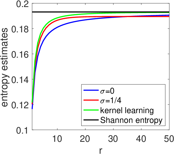
Note that as a consequence of Jensen’s inequality, we always have 𝔼⁡(tr[Σ^p​log⁡Σ^p])⩾tr[Σp​log⁡Σp]{\mathbb{E}}\big(\mathop{\rm tr}\big[\hat{\Sigma}_{p}\log\hat{\Sigma}_{p}\big]\big)\geqslant\mathop{\rm tr}\big[{\Sigma}_{p}\log{\Sigma}_{p}\big], as can be seen in simulations (see Figure 1).

5.3 Examples

We consider the dd-dimensional torus [0,1]d[0,1]^{d} with a translation-invariant kernel k⁡(x,y)=k⁡(x−y)k(x,y)=k(x-y) with k^​(ω)=k^​(0)​e−σ​‖ω‖1\hat{k}(\omega)=\hat{k}(0)e^{-\sigma\|\omega\|_{1}}. We have by symmetry ⟨φ⁡(x),(Σ+λ​I)−1​φ​(x)⟩=tr[Σ​(Σ+λ​I)−1]=∑ω∈ℤdk^​(ω)k^​(ω)+λ.\displaystyle\langle\varphi(x),(\Sigma+\lambda I)^{-1}\varphi(x)\rangle=\mathop{\rm tr}\big[\Sigma(\Sigma+\lambda I)^{-1}\big]=\sum_{\omega\in{\mathbb{Z}}^{d}}\frac{\hat{k}(\omega)}{\hat{k}(\omega)+\lambda}. As shown in Appendix C.6, we have the bound tr[Σ(Σ+λI)−1]⩽e−σd/2d!sinhd⁡(σ/2)[1+(logtanhd⁡σ2λ)d]\displaystyle\mathop{\rm tr}\big[\Sigma(\Sigma+\lambda I)^{-1}\big]\leqslant e^{-\sigma d/2}\frac{d!}{\sinh^{d}(\sigma/2)}\Big[1+\Big(\log\frac{\tanh^{d}\frac{\sigma}{2}}{\lambda}\Big)^{d}\Big]. Thus, the constant cc in Prop. 7 above can be upper bounded by a constant times σ−d\sigma^{-d} (see Appendix C.6 for details). We thus get an overall estimation rate for the kernel entropy proportional to σ−d/2n\sigma^{-d/2}{\sqrt{n}}.

When balancing with the O⁡(σ2)O(\sigma^{2}) estimation of the entropy for Lipschitz-continuous strictly positive densities in Section 4.2, we can take σ∝n−1/(d+4)\sigma\propto{n^{-1/(d+4)}} (lower bandwidth with more observations), leading to a rate of n−2/(d+4){n^{-2/(d+4)}}, which is to be compared to the optimal rate equal to n−4/(d+4){n^{-4/(d+4)}} for entropy estimation for densities with the same regularity [28]. Although our primary goal was not to estimate entropies, we get a rate which is the square root of the optimal rate.

Illustrative experiments.

We consider 𝒳=[0,1]{\mathcal{X}}=[0,1] and p⁡(x)=4​|x−12|p(x)=4\big|x-\frac{1}{2}\big|, with negative differential entropy ∫01p⁡(x)​log⁡p⁡(x)​𝑑x=log⁡2−12≈0.1931\displaystyle\int_{0}^{1}p(x)\log p(x)dx=\log 2-\frac{1}{2}\approx 0.1931. We consider estimation from various numbers of i.i.d. observations. See left plot in Figure 1, where we compare two values of σ\sigma. Note that the estimation is empirically here in expectation from above, as expected because of Jensen’s inequality (as opposed to the right plot).

Refer to caption
Refer to caption
Figure 1: Negative entropy estimation from 20 replications (mean and standard deviation) for two values of the kernel bandwidth σ\sigma, as nn increases. Left: from i.i.d. samples (method from Section 5.1). Right: from kernel integrals evaluated as uniform samples (method from Section 5.4). As expected we estimate the kernel entropy (limit when nn tends to infinity) from above on the left plot, and from below on the right plot, with a faster convergence rate on the right plot.

5.4 Estimation from other oracles

If we have access to other oracles on pp and qq, we can consider other estimators.1111 11 This section is not crucial to understand the rest of the paper. For example, if we can estimate ∫𝒳k⁡(x,y)​k​(x,z)​𝑑p​(x)\int_{\mathcal{X}}k(x,y)k(x,z)dp(x) and ∫𝒳k⁡(x,y)​k​(x,z)​𝑑q​(x)\int_{\mathcal{X}}k(x,y)k(x,z)dq(x) for any y,z∈𝒳y,z\in{\mathcal{X}}, we can simply sample nn points x1,…,xnx_{1},\dots,x_{n} from the base measure on 𝒳{\mathcal{X}}, and, given the projection operator Π^\hat{\Pi} on the span of φ⁡(x1),…,φ⁡(xn)\varphi(x_{1}),\dots,\varphi(x_{n}), consider

Σ^p=Π^​Σp​Π^​ and ​Σ^q=Π^​Σq​Π^,\hat{\Sigma}_{p}=\hat{\Pi}{\Sigma}_{p}\hat{\Pi}\mbox{ and }\hat{\Sigma}_{q}=\hat{\Pi}{\Sigma}_{q}\hat{\Pi}, (12)

and the estimator D(Σ^p∥Σ^q)D(\hat{\Sigma}_{p}\|\hat{\Sigma}_{q}) which is now a pointwise lower bound1212 12 Since Π^​Π^∗+(I−Π^)​(I−Π^)∗=I\hat{\Pi}\hat{\Pi}^{\ast}+(I-\hat{\Pi})(I-\hat{\Pi})^{\ast}=I, the monotonicity of relative entropy (Prop. 14 in Appendix A.2) leads to D(Σp∥Σq)⩾D(Π^ΣpΠ^+(I−Π^)Σp(I−Π^)∥Π^ΣqΠ^+(I−Π^)Σq(I−Π^))=D(Π^ΣpΠ^∥Π^ΣqΠ^)+D((I−Π^)Σp(I−Π^)∥(I−Π^)Σq(I−Π^))D(\Sigma_{p}\|\Sigma_{q})\geqslant D\big(\hat{\Pi}{\Sigma}_{p}\hat{\Pi}+(I-\hat{\Pi}){\Sigma}_{p}(I-\hat{\Pi})\big\|\hat{\Pi}{\Sigma}_{q}\hat{\Pi}+(I-\hat{\Pi}){\Sigma}_{q}(I-\hat{\Pi})\big)=D\big(\hat{\Pi}{\Sigma}_{p}\hat{\Pi}\|\hat{\Pi}{\Sigma}_{q}\hat{\Pi}\big)+D\big((I-\hat{\Pi}){\Sigma}_{p}(I-\hat{\Pi})\|(I-\hat{\Pi}){\Sigma}_{q}(I-\hat{\Pi})\big), which is greater than D(Π^ΣpΠ^∥Π^ΣqΠ^)D\big(\hat{\Pi}{\Sigma}_{p}\hat{\Pi}\|\hat{\Pi}{\Sigma}_{q}\hat{\Pi}\big). on D(Σp∥Σq)D({\Sigma}_{p}\|{\Sigma}_{q}) (and thus on D(p∥q)D(p\|q)), which can be beneficial in variational inference, as presented in Section 7.

Noting that ⟨φ⁡(xi),Σp​φ​(xj)⟩=∫𝒳k⁡(xi,x)​k​(x,xj)​𝑑p​(x)\langle\varphi(x_{i}),\Sigma_{p}\varphi(x_{j})\rangle=\int_{\mathcal{X}}k(x_{i},x)k(x,x_{j})dp(x) (and similarly for Σq\Sigma_{q}), and that KK is the matrix of dot-products of φ⁡(x1),…,φ⁡(xn)\varphi(x_{1}),\dots,\varphi(x_{n}), the orthogonal projection may be done as

D(Σ^p∥Σ^q)=D(K−1/2∫𝒳k(X,x)k(x,X)dp(x)K−1/2∥K−1/2∫𝒳k(X,x)k(x,X)dq(x)K−1/2),D(\hat{\Sigma}_{p}\|\hat{\Sigma}_{q})=D\Big(K^{-1/2}\int_{\mathcal{X}}k(X,x)k(x,X)dp(x)K^{-1/2}\Big\|K^{-1/2}\int_{\mathcal{X}}k(X,x)k(x,X)dq(x)K^{-1/2}\Big),

where k⁡(X,x)∈ℝnk(X,x)\in\mathbb{R}^{n} is the vector with components k⁡(xi,x)k(x_{i},x), i=1,…,ni=1,\dots,n, and K∈ℝn×nK\in\mathbb{R}^{n\times n} the kernel matrix, typically with some added regularization for numetical stability, and incomplete Cholesky decomposition so as to minimize the number of kernel evaluations (see, e.g., [7] and references therein), with an overall running time complexity of O⁡(n3)O(n^{3}). A key property is that it always underestimates the kernel relative entropy (and hence the Shannon relative entropy). The following proposition shows that it provides a better estimate (better dependence in nn) than with i.i.d. samples (see proof in Appendix C.5).

Proposition 8

Assume (A1) and that p{p} has a density with respect to the base measure which is bounded. Given uniform i.i.d. samples x1,…,xnx_{1},\dots,x_{n} from the base distribution, and the estimator defined by Eq. (12), we have, if for all λ>0\lambda>0, supx∈𝒳⟨φ⁡(x),(Σ+λ​I)−1​φ​(x)⟩⩽B​log⁡(C/λ)d\sup_{x\in{\mathcal{X}}}\,\langle\varphi(x),(\Sigma+\lambda I)^{-1}\varphi(x)\rangle\leqslant B\log(C/\lambda)^{d}, for some constants B,CB,C:

0⩽tr[Π^​Σp​Π^​log⁡(Π^​Σp​Π^)]−tr[Σp​log⁡Σp]=O⁡((log⁡(B​C))d​(B​C+B)​exp⁡(−14​(B​n)1/(d+1))).0\leqslant\mathop{\rm tr}\big[\hat{\Pi}{\Sigma}_{p}\hat{\Pi}\log(\hat{\Pi}{\Sigma}_{p}\hat{\Pi})\big]-\mathop{\rm tr}\big[{\Sigma}_{p}\log{\Sigma}_{p}\big]=O\Big(\big(\log(BC)\big)^{d}(\sqrt{BC}+B)\exp\big(-\frac{1}{4}(Bn)^{1/(d+1)}\big)\Big).

The proposition above applies to the torus situation in [0,1]d[0,1]^{d} and the kernel with exponential Fourier series, with now an improved dependence in nn and in dd, since in that case B∼C∼σdB\sim C\sim\sigma^{d}. That is, to reach precision ε\varepsilon, we need n∝σ−d​(log⁡σdε)d+1n\propto\sigma^{-d}\big(\log\frac{\sigma^{d}}{\varepsilon}\big)^{d+1} instead of n∼σ−d​ε−2n~\sim{\sigma^{-d}\varepsilon^{-2}}. Other decays for the maximal degrees of freedom are considered in Appendix C.5.

Illustrative experiments.

We consider as above p⁡(x)=4​|x−12|p(x)=4\big|x-\frac{1}{2}\big|, and consider estimation from various numbers of i.i.d. observations for the projection. The required integrals are computed by numerical integration. See right plot in Figure 1, where we compare two values of σ\sigma. Note that the estimation is as expected here from below, and with a faster rate of convergence than for the estimation method from Section 5.1.

6 Multivariate probabilistic modelling

Information-theoretic quantities are particularly useful at characterizing statistical dependence between random variables. This is for example the basis of independent component analysis [17], and can be used for feature selection [51]. We explore how the new notions of entropy can be used in this goal.

6.1 Joint entropy, marginal entropy and mutual information

We assume that we have a product set 𝒳=𝒳1×𝒳2{\mathcal{X}}={\mathcal{X}}_{1}\times{\mathcal{X}}_{2}, and a feature space ℋ=ℋ1⊗ℋ2{\mathcal{H}}={\mathcal{H}}_{1}\otimes{\mathcal{H}}_{2}, corresponding to the kernel k⁡(x,y)=k1​(x1,y1)​k2​(x2,y2)k(x,y)=k_{1}(x_{1},y_{1})k_{2}(x_{2},y_{2}), and feature map φ⁡(x)=φ1​(x1)⊗φ2​(x2)\varphi(x)=\varphi_{1}(x_{1})\otimes\varphi_{2}(x_{2}). We also consider a base distribution on 𝒳1×𝒳2{\mathcal{X}}_{1}\times{\mathcal{X}}_{2} which is the product of the base distributions. The tensor product is here defined as the span of all functions (x1,x2)↦f1​(x1)​f2​(x2)(x_{1},x_{2})\mapsto f_{1}(x_{1})f_{2}(x_{2}) for fi∈ℋif_{i}\in{\mathcal{H}}_{i}, i=1,2i=1,2, with the norm ‖f1‖⋅‖f2‖\|f_{1}\|\cdot\|f_{2}\|. Given a joint probability pX1​X2p_{X_{1}X_{2}} and its marginal probability distributions pX1p_{X_{1}} and pX2p_{X_{2}}, we can define the covariance operators ΣpX1​X2\Sigma_{p_{X_{1}X_{2}}} on ℋ1⊗ℋ2{\mathcal{H}}_{1}\otimes{\mathcal{H}}_{2}, ΣpX1\Sigma_{p_{X_{1}}} on ℋ1{\mathcal{H}}_{1}, and ΣpX2\Sigma_{p_{X_{2}}} on ℋ2{\mathcal{H}}_{2}, as well as Σ12\Sigma_{12}, Σ1\Sigma_{1} and Σ2\Sigma_{2} the covariance operators of the base distributions on 𝒳1×𝒳2{\mathcal{X}}_{1}\times{\mathcal{X}}_{2}, 𝒳1{\mathcal{X}}_{1} and 𝒳2{\mathcal{X}}_{2}:

We then define the marginal and joint entropies as:

H⁡(ΣpX1)\displaystyle H(\Sigma_{p_{X_{1}}}) =\displaystyle= −tr[ΣpX1logΣpX1]+tr[ΣpX1logΣ1]−minx1∈𝒳1⟨φ1(x1),(logΣ1)φ1(x1)⟩\displaystyle-\mathop{\rm tr}\big[\Sigma_{p_{X_{1}}}\log\Sigma_{p_{X_{1}}}\big]+\mathop{\rm tr}\big[\Sigma_{p_{X_{1}}}\log\Sigma_{1}\big]-\min_{x_{1}\in{\mathcal{X}}_{1}}\langle\varphi_{1}(x_{1}),(\log\Sigma_{1})\varphi_{1}(x_{1})\rangle
H⁡(ΣpX2)\displaystyle H(\Sigma_{p_{X_{2}}}) =\displaystyle= −tr[ΣpX2logΣpX2]+tr[ΣpX2logΣ2]−minx2∈𝒳2⟨φ2(x2),(logΣ2)φ2(x2)⟩\displaystyle-\mathop{\rm tr}\big[\Sigma_{p_{X_{2}}}\log\Sigma_{p_{X_{2}}}\big]+\mathop{\rm tr}\big[\Sigma_{p_{X_{2}}}\log\Sigma_{2}\big]-\min_{x_{2}\in{\mathcal{X}}_{2}}\langle\varphi_{2}(x_{2}),(\log\Sigma_{2})\varphi_{2}(x_{2})\rangle
H⁡(ΣpX1​X2)\displaystyle H(\Sigma_{p_{X_{1}X_{2}}}) =\displaystyle= −tr[ΣpX1​X2logΣpX1​X2]+tr[ΣpX1​X2logΣ12]−minx∈𝒳⟨φ(x),(logΣ12)φ(x)⟩.\displaystyle-\mathop{\rm tr}\big[\Sigma_{p_{X_{1}X_{2}}}\log\Sigma_{p_{X_{1}X_{2}}}\big]+\mathop{\rm tr}\big[\Sigma_{p_{X_{1}X_{2}}}\log\Sigma_{12}\big]-\min_{x\in{\mathcal{X}}}\langle\varphi(x),(\log\Sigma_{12})\varphi(x)\rangle.

The product distribution pX1​pX2p_{X_{1}}p_{X_{2}} (with independent components with same marginal distributions as XX), which is different in general from the joint distribution pX1​X2p_{X_{1}X_{2}}, has covariance operator ΣpX1​pX2=ΣpX1⊗ΣpX2\Sigma_{p_{X_{1}}p_{X_{2}}}=\Sigma_{p_{X_{1}}}\otimes\Sigma_{p_{X_{2}}}, and its entropy is:

H⁡(ΣpX1​pX2)\displaystyle H(\Sigma_{p_{X_{1}}p_{X_{2}}}) =\displaystyle= −tr[ΣpX1⊗ΣpX2logΣpX1⊗ΣpX2]+tr[ΣpX1⊗ΣpX2logΣ12]−minx∈𝒳⟨φ(x),(logΣ12)φ(x)⟩.\displaystyle-\mathop{\rm tr}\big[\Sigma_{p_{X_{1}}}\otimes\Sigma_{p_{X_{2}}}\log\Sigma_{p_{X_{1}}}\otimes\Sigma_{p_{X_{2}}}\big]+\mathop{\rm tr}\big[\Sigma_{p_{X_{1}}}\otimes\Sigma_{p_{X_{2}}}\log\Sigma_{12}\big]-\min_{x\in{\mathcal{X}}}\langle\varphi(x),(\log\Sigma_{12})\varphi(x)\rangle.

We have log⁡ΣpX1⊗ΣpX2=log⁡ΣpX1⊗I+log⁡I⊗ΣpX2\log\Sigma_{p_{X_{1}}}\otimes\Sigma_{p_{X_{2}}}=\log\Sigma_{p_{X_{1}}}\otimes I+\log I\otimes\Sigma_{p_{X_{2}}}. Moreover, because the base distribution is separable by assumption, we have ⟨φ⁡(x),(log⁡Σ12)​φ​(x)⟩=⟨φ1​(x1),(log⁡Σ1)​φ1​(x1)⟩+⟨φ2​(x2),(log⁡Σ2)​φ2​(x2)⟩\langle\varphi(x),(\log\Sigma_{12})\varphi(x)\rangle=\langle\varphi_{1}(x_{1}),(\log\Sigma_{1})\varphi_{1}(x_{1})\rangle+\langle\varphi_{2}(x_{2}),(\log\Sigma_{2})\varphi_{2}(x_{2})\rangle, thus, we exactly have:

H⁡(ΣpX1​pX2)=H⁡(ΣpX1)+H⁡(ΣpX2).H(\Sigma_{p_{X_{1}}p_{X_{2}}})=H(\Sigma_{p_{X_{1}}})+H(\Sigma_{p_{X_{2}}}).

We can therefore define the kernel mutual information (not to be confused with the regular Shannon mutual information) as

I(X1,X2)=D(ΣpX1​X2∥ΣpX1⊗ΣpX2).I(X_{1},X_{2})=D(\Sigma_{p_{X_{1}X_{2}}}\|\Sigma_{p_{X_{1}}}\otimes\Sigma_{p_{X_{2}}}).

From the developments above, it is equal to

I⁡(X1,X2)=H⁡(ΣpX1)+H⁡(ΣpX2)−H⁡(ΣpX1​X2),I(X_{1},X_{2})=H(\Sigma_{p_{X_{1}}})+H(\Sigma_{p_{X_{2}}})-H(\Sigma_{p_{X_{1}X_{2}}}),

mimicking the traditional equality for regular entropies. Moreover, it is equal to zero if and only if the variables are independent.

Proposition 9 (Characterization of independence)

Assume (A1). Then I⁡(X1,X2)I(X_{1},X_{2}) is a lower bound on the Shannon mutual information, and I⁡(X1,X2)=0I(X_{1},X_{2})=0 if and only if ΣpX1​X2=ΣpX1⊗ΣpX2\Sigma_{p_{X_{1}X_{2}}}=\Sigma_{p_{X_{1}}}\otimes\Sigma_{p_{X_{2}}}. If the kernel k2k^{2} is universal, this is equivalent to the random variables X1X_{1} and X1X_{1} being independent.

Proof The first statement is straightforward because of the interpretation as a relative entropy. The second statement is simply the consequence of the fact that ΣpX1⊗ΣpX2\Sigma_{p_{X_{1}}}\otimes\Sigma_{p_{X_{2}}} is the covariance operator of the product distribution pX1​pX2p_{X_{1}}p_{X_{2}}.  
We can make the following observations:

  • •

    The extension to mutual information between more than two random variables is straightforward by considering tensor products between all marginals, with the same characterization property of independence.

  • •

    Our use of covariance operators is related to the “kernel generalized variance” from [6], which considers a joint covariance operator (𝔼⁡[φ1​(X1)​φ1​(X1)∗]𝔼⁡[φ1​(X1)​φ2​(X2)∗]𝔼⁡[φ2​(X2)​φ1​(X1)∗]𝔼⁡[φ2​(X2)​φ2​(X2)∗])=𝔼⁡[(φ1​(X1)φ2​(X2))​(φ1​(X1)φ2​(X2))∗]\displaystyle\bigg(\begin{array}[]{cc}{\mathbb{E}}\big[\varphi_{1}(X_{1})\varphi_{1}(X_{1})^{\ast}\big]&{\mathbb{E}}\big[\varphi_{1}(X_{1})\varphi_{2}(X_{2})^{\ast}\big]\\ {\mathbb{E}}\big[\varphi_{2}(X_{2})\varphi_{1}(X_{1})^{\ast}\big]&{\mathbb{E}}\big[\varphi_{2}(X_{2})\varphi_{2}(X_{2})^{\ast}\big]\end{array}\bigg)={\mathbb{E}}\bigg[{\varphi_{1}(X_{1})\choose\varphi_{2}(X_{2})}{\varphi_{1}(X_{1})\choose\varphi_{2}(X_{2})}^{\ast}\bigg], and compute the mutual information for a Gaussian vector with this covariance operator. The kernel generalized variance can be generalized to more than two random variables, but then the independence characterization property is not satisfied. Moreover, the relationship with the usual mutual information is not as straightforward.

  • •

    The extension to conditional entropies is not straightforward. We could define ΣpX2|X1=x1\Sigma_{p_{X_{2}|X_{1}=x_{1}}} in the natural way, but then we do not have the joint entropy being the sum of the marginal and conditional entropy (otherwise, because of axiomatic characterizations of entropy [20], we would get back exactly the Shannon entropy). There is also a potential for exponential families and conditional models akin to generalized models, which remains to be explored.

6.2 Data processing inequality

We have a form of data processing inequality, which is classical in quantum information theory (see, e.g., [40]), which we extend here.

Proposition 10 (Data processing inequality)

Assume (A1). We have

D(ΣpX1​X2∥ΣqX1​X2)⩾D(ΣpX1∥ΣqX1),D(\Sigma_{p_{X_{1}X_{2}}}\|\Sigma_{q_{X_{1}X_{2}}})\geqslant D(\Sigma_{p_{X_{1}}}\|\Sigma_{q_{X_{1}}}),

with equality implying (when the kernel kk is universal) that the conditional distribution of X2X_{2} given X1X_{1} is the same for pp and qq, but the reverse implication is not true in general.

Proof The marginal operators ΣpX1\Sigma_{p_{X_{1}}} and ΣqX1\Sigma_{q_{X_{1}}} are obtained by taking “partial traces” which are quantum operations as defined in Section 3, hence the inequality. Following [46], we have inequality if and only log⁡ΣpX1​X2−log⁡ΣpX1​X2=log⁡(ΣpX1⊗I)−log⁡(ΣqX1⊗I)\log\Sigma_{p_{X_{1}X_{2}}}-\log\Sigma_{p_{X_{1}X_{2}}}=\log(\Sigma_{p_{X_{1}}}\otimes I)-\log(\Sigma_{q_{X_{1}}}\otimes I), which is unfortunately not always satisfied when conditional distributions are equal. However, in case of equality, the extra condition (c) from Prop. 2, becomes ΣpX1​X2​(ΣqX1⊗I)=ΣqX1​X2​(ΣpX1⊗I)\Sigma_{p_{X_{1}X_{2}}}(\Sigma_{q_{X_{1}}}\otimes I)=\Sigma_{q_{X_{1}X_{2}}}(\Sigma_{p_{X_{1}}}\otimes I), and can be leveraged. Indeed, for all test functions f1,g1,f2,g2f_{1},g_{1},f_{2},g_{2} in ℋ{\mathcal{H}}, it leads to:

∫𝒳1×𝒳2∫𝒳1f1​(x1)​f2​(x2)​g1​(y1)​g2​(y2)​k1​(x1,y1)​d​pX1​X2​(x1,x2)​d​qX1​(y1)\int_{{\mathcal{X}}_{1}\times{\mathcal{X}}_{2}}\int_{{\mathcal{X}}_{1}}f_{1}(x_{1})f_{2}(x_{2})g_{1}(y_{1})g_{2}(y_{2})k_{1}(x_{1},y_{1})dp_{X_{1}X_{2}}(x_{1},x_{2})dq_{X_{1}}(y_{1})
=∫𝒳1×𝒳2∫𝒳1f1​(x1)​f2​(x2)​g1​(y1)​g2​(y2)​k1​(x1,y1)​d​qX1​X2​(x1,x2)​d​p1​(y1).=\int_{{\mathcal{X}}_{1}\times{\mathcal{X}}_{2}}\int_{{\mathcal{X}}_{1}}f_{1}(x_{1})f_{2}(x_{2})g_{1}(y_{1})g_{2}(y_{2})k_{1}(x_{1},y_{1})dq_{X_{1}X_{2}}(x_{1},x_{2})dp_{1}(y_{1}).

Considering f1f_{1} and g1g_{1} tending to Dirac functions at x¯1\bar{x}_{1} (which is possible since the kernel is univeral) we get ∫𝒳2f2​(x2)​g2​(y2)​d​pX1​X2​(x¯1,x2)​d​qX1​(x¯1)=∫𝒳2f2​(x2)​g2​(y2)​d​qX1​X2​(x¯1,x2)​d​p1​(x¯1),\int_{{\mathcal{X}}_{2}}f_{2}(x_{2})g_{2}(y_{2})dp_{X_{1}X_{2}}(\bar{x}_{1},x_{2})dq_{X_{1}}(\bar{x}_{1})=\int_{{\mathcal{X}}_{2}}f_{2}(x_{2})g_{2}(y_{2})dq_{X_{1}X_{2}}(\bar{x}_{1},x_{2})dp_{1}(\bar{x}_{1}), which implies that the conditional distributions of x2x_{2} given x1x_{1} is the same for pp and qq.  

6.3 Submodularity and conditional independence

We can now consider three variables X1,X2,X3X_{1},X_{2},X_{3}, and use strong sub-additivity of the quantum relative entropy [46, 40].

Proposition 11 (Submodularity)

Assume (A1). We have:

H⁡(ΣpX1​X2​X3)−H⁡(ΣpX1​X2)−H⁡(ΣpX2​X3)+H⁡(ΣpX2)⩽0,H(\Sigma_{p_{X_{1}X_{2}X_{3}}})-H(\Sigma_{p_{X_{1}X_{2}}})-H(\Sigma_{p_{X_{2}X_{3}}})+H(\Sigma_{p_{X_{2}}})\leqslant 0,

with equality (for universal kernels) implying that X1X_{1} and X3X_{3} are independent given X2X_{2}, but in general the reverse implication is not true.

Proof As done by [40], we can simply apply the data processing result (Prop. 10) to X~1=(X1,X2),\tilde{X}_{1}=(X_{1},X_{2}), and X~2=X3\tilde{X}_{2}=X_{3}, with the distributions p~X~1​X~2=pX1​X2​X3\tilde{p}_{\tilde{X}_{1}\tilde{X}_{2}}=p_{X_{1}X_{2}X_{3}} and q~X~1​X~2=pX1​pX2​X3\tilde{q}_{\tilde{X}_{1}\tilde{X}_{2}}=p_{X_{1}}p_{X_{2}X_{3}}.  
As a classical consequence, the entropy function is submodular like the regular entropy (see, e.g., [3, Section 6.5]).

Note that we do not obtain a necessary and sufficient characterization of conditional independence, which can be obtained with other tools based on covariance operators [27].

7 Convex duality, log-partition functions and variational inference

Given that our kernel notions of relative entropies are lower bounds on the regular notions, by the traditional convex duality results between maximum entropy and log-partition functions (see, e.g., [58]), we should obtain upper-bounds on log-partition functions. In this section, we show how such bounds can be obtained and computed. We then show that such bounds can also be optimized with respect to the positive definite kernel.

This leads to a new family of variational inference methods, which can then be used in various probabilistic inference tasks [58], and in particular in Bayesian inference [42].

In this section, we will sometimes only assume that for our kernels satisfy (on top of being positive definite) k⁡(x,x)⩽1k(x,x)\leqslant 1 for all x∈𝒳x\in{\mathcal{X}}, noting that the upper-bound result on the regular Shannon relative entropy is still valid in this case.

7.1 Convex duality between operators

We have for self-adjoint operators (regardless of the link with input spaces and probabilities):

supA≽0,trA=1tr(AM)−D(A∥B)\displaystyle\sup_{A\succcurlyeq 0,\ \mathop{\rm tr}A=1}\mathop{\rm tr}(AM)-D(A\|B) =\displaystyle= supA≽0,trA=1tr(A⁡(M+log⁡B))−tr[A​log⁡A]\displaystyle\sup_{A\succcurlyeq 0,\ \mathop{\rm tr}A=1}\mathop{\rm tr}(A(M+\log B))-\mathop{\rm tr}[A\log A]
=\displaystyle= logtrexp(M+logB),\displaystyle\log\mathop{\rm tr}\exp(M+\log B),

with the optimal operator AA equal to A=1trexp⁡(M+log⁡B)​exp⁡(M+log⁡B)\displaystyle A=\frac{1}{\mathop{\rm tr}\exp(M+\log B)}\exp(M+\log B). This implies the representation

D(A∥B)=supMtrAM−logtrexp(M+logB),D(A\|B)=\sup_{M}\ \mathop{\rm tr}AM-\log\mathop{\rm tr}\exp(M+\log B),

with the constraints that A≽0A\succcurlyeq 0 and trA=1\mathop{\rm tr}A=1 are automatically satisfied (if trA≠1\mathop{\rm tr}A\neq 1, then by replacing MM by M+t​IM+tI, we can make the quantity go to infinity).

We also have (when the constraint for unit trace is removed):

supA≽0tr(AM)−D(A∥B)\displaystyle\sup_{A\succcurlyeq 0}\mathop{\rm tr}(AM)-D(A\|B) =\displaystyle= supA≽0tr(A⁡(M+log⁡B))−tr[A​log⁡A]\displaystyle\sup_{A\succcurlyeq 0}\mathop{\rm tr}(A(M+\log B))-\mathop{\rm tr}[A\log A]
=\displaystyle= trexp⁡(M+log⁡B−I),\displaystyle\mathop{\rm tr}\exp(M+\log B-I),

with an optimal A=1e​exp⁡(M+log⁡B)A=\frac{1}{e}\exp(M+\log B). This implies the representation

D(A∥B)=supMtrA+trAM−trexp(M+logB),D(A\|B)=\sup_{M}\ \mathop{\rm tr}A+\mathop{\rm tr}AM-\mathop{\rm tr}\exp(M+\log B),

with the constraint that A≽0A\succcurlyeq 0 is automatically satisfied (but not trA=1\mathop{\rm tr}A=1), with the optimal MM equal to log⁡A−log⁡B\log A-\log B.

7.2 Bounds on the log-partition function

We can now apply the duality relationships above to covariance operators. Given a bounded function f:𝒳→ℝf:{\mathcal{X}}\to\mathbb{R} and a distribution qq on 𝒳{\mathcal{X}}, our goal is to obtain upper-bounds on the log-partition function log∫𝒳ef⁡(x)dq(x)\log\int_{\mathcal{X}}e^{f(x)}dq(x) which is equal to, by convex duality:

log∫𝒳ef⁡(x)dq(x)=supp​probability∫𝒳f(x)dp(x)−D(p∥q).\log\int_{\mathcal{X}}e^{f(x)}dq(x)=\sup_{p\ {\rm probability}}\int_{\mathcal{X}}f(x)dp(x)-D(p\|q).

In our situation, our operators are subject to belong to the subspace 𝒜{\mathcal{A}}, equal to the span of all φ⁡(x)​φ​(x)∗\varphi(x)\varphi(x)^{\ast}, for x∈𝒳x\in{\mathcal{X}}, which leads to slight adaptations. We do not necessarily assume that the kernels are universal, so that the hull of all φ⁡(x)​φ​(x)∗\varphi(x)\varphi(x)^{\ast} may not be equal to the intersection of 𝒜{\mathcal{A}} and positive operators with unit trace.

Isotropic kernels.

If k⁡(x,x)=1k(x,x)=1, for all x∈𝒳x\in{\mathcal{X}}, then trΣp=1\mathop{\rm tr}\Sigma_{p}=1 is equivalent to ∫𝒳d​p​(x)=1\int_{\mathcal{X}}dp(x)=1. We define for a bounded function f:𝒳→ℝf:{\mathcal{X}}\to\mathbb{R},

a(f)=supp​probability​measure∫𝒳f(x)dp(x)−D(Σp∥Σq).a(f)=\sup_{p\ {\rm probability\ measure}}\int_{\mathcal{X}}f(x)dp(x)-D(\Sigma_{p}\|\Sigma_{q}).

Using convex duality tools from Section 7.1, we have:

a⁡(f)\displaystyle a(f) =\displaystyle= supp​non−negative​measureinfM∫𝒳f(x)dp(x)−trΣpM+logtrexp(M+logΣq)\displaystyle\sup_{p\ {\rm non-negative\ measure}}\inf_{M}\int_{\mathcal{X}}f(x)dp(x)-\mathop{\rm tr}\Sigma_{p}M+\log\mathop{\rm tr}\exp(M+\log\Sigma_{q})
=\displaystyle= infMlogtrexp(M+logΣq) such that ∀x∈𝒳,f(x)⩽⟨φ(x),Mφ(x)⟩.\displaystyle\inf_{M}\log\mathop{\rm tr}\exp(M+\log\Sigma_{q})\mbox{ such that }\forall x\in{\mathcal{X}},\ f(x)\leqslant\langle\varphi(x),M\varphi(x)\rangle.

Note that we can get rid of the constraint ∫𝒳d​p​(x)=1\int_{\mathcal{X}}dp(x)=1 because it is equivalent to trΣp=1\mathop{\rm tr}\Sigma_{p}=1.

A relaxation is to relax pp not to be a non-negative measure (and use the positivity of Σp\Sigma_{p} as the only constraint), leading to

b(f)=supp​measure∫𝒳f(x)dp(x)−D(Σq∥Σq).b(f)=\sup_{p\ {\rm measure}}\ \int_{\mathcal{X}}f(x)dp(x)-D(\Sigma_{q}\|\Sigma_{q}). (13)

By construction, we have a⁡(f)⩽b⁡(f)a(f)\leqslant b(f), and by convex duality,

b⁡(f)\displaystyle b(f) =\displaystyle= supp​measureinfM∫𝒳f(x)dp(x)−trΣpM+logtrexp(M+logΣq)\displaystyle\sup_{p\ {\rm measure}}\inf_{M}\int_{\mathcal{X}}f(x)dp(x)-\mathop{\rm tr}\Sigma_{p}M+\log\mathop{\rm tr}\exp(M+\log\Sigma_{q}) (14)
=\displaystyle= infMlogtrexp(M+logΣq) such that ∀x∈𝒳,f(x)=⟨φ(x),Mφ(x)⟩.\displaystyle\inf_{M}\ \log\mathop{\rm tr}\exp(M+\log\Sigma_{q})\mbox{ such that }\forall x\in{\mathcal{X}},\ f(x)=\langle\varphi(x),M\varphi(x)\rangle.

Note that that if the problem above is non-feasible because φ\varphi is too small (so that ff cannot be represented as a quadratic form in φ\varphi), then we get a value +∞+\infty.

If we can write (usually non-uniquely), f⁡(x)=⟨φ⁡(x),F​φ​(x)⟩f(x)=\langle\varphi(x),F\varphi(x)\rangle for some self-adjoint operator FF, then we have another representation as:

b⁡(f)\displaystyle b(f) =\displaystyle= infN∈𝒜⟂logtrexp(F+N+logΣq).\displaystyle\inf_{N\in\mathcal{A}^{\perp}}\ \log\mathop{\rm tr}\exp(F+N+\log\Sigma_{q}).

Since D(Σp∥Σq)⩽D(p∥q)D(\Sigma_{p}\|\Sigma_{q})\leqslant D(p\|q), we have:

b(f)⩾a(f)⩾supp​probability∫𝒳f(x)dp(x)−D(p∥q)=log∫𝒳ef⁡(x)dq(x).b(f)\geqslant a(f)\geqslant\sup_{p\ {\rm probability}}\int_{\mathcal{X}}f(x)dp(x)-D(p\|q)=\log\int_{\mathcal{X}}e^{f(x)}dq(x).

As expected, we thus obtain upper bounds on the usual log-partition function.

Note that we could also get lower bounds using tools from Section 4.1, in particular for functions ff that can be written as f⁡(x)=∫𝒳h⁡(x,y)​g​(y)​𝑑τ​(y)f(x)=\int_{\mathcal{X}}h(x,y)g(y)d\tau(y).

Non isotropic kernels.

If we only assume that k⁡(x,x)⩽1k(x,x)\leqslant 1 for all x∈𝒳x\in{\mathcal{X}}, then b⁡(f)b(f) defined in Eq. (13) and Eq. (14) is not any more an upper-bound but we can define instead

b(c)​(f)\displaystyle b^{(c)}(f) =\displaystyle= supp​measure,∫𝒳d​p​(x)=1,∫𝒳k⁡(x,x)​𝑑p​(x)⩽1infM∫𝒳f⁡(x)​𝑑p​(x)−trΣp​M−trΣp+trexp⁡(M+log⁡Σq)\displaystyle\sup_{p\ {\rm measure},\ \int_{\mathcal{X}}dp(x)=1,\ \int_{\mathcal{X}}k(x,x)dp(x)\leqslant 1}\inf_{M}\int_{\mathcal{X}}f(x)dp(x)-\mathop{\rm tr}\Sigma_{p}M-\mathop{\rm tr}\Sigma_{p}+\mathop{\rm tr}\exp(M+\log\Sigma_{q})
=\displaystyle= supp​measureinfM,c,b⩾0∫𝒳f⁡(x)​𝑑p​(x)−trΣp​M−trΣp+trexp⁡(M+log⁡Σq)\displaystyle\sup_{p\ {\rm measure}}\inf_{M,\,c,\,b\geqslant 0}\int_{\mathcal{X}}f(x)dp(x)-\mathop{\rm tr}\Sigma_{p}M-\mathop{\rm tr}\Sigma_{p}+\mathop{\rm tr}\exp(M+\log\Sigma_{q})
−c⁡(∫𝒳d​p​(x)−1)−b⁡(∫𝒳k⁡(x,x)​𝑑p​(x)−1)\displaystyle\hskip 170.71652pt-c\Big(\int_{\mathcal{X}}dp(x)-1\Big)-b\Big(\int_{\mathcal{X}}k(x,x)dp(x)-1\Big)
=\displaystyle= infM,c,b⩾0c+b+trexp⁡(M+log⁡Σq)​ such that ​∀x∈𝒳,f⁡(x)=c+⟨φ⁡(x),(M+I+b​I)​φ​(x)⟩\displaystyle\inf_{M,\,c,\,b\geqslant 0}\ c+b+\mathop{\rm tr}\exp(M+\log\Sigma_{q})\mbox{ such that }\forall x\in{\mathcal{X}},\ f(x)=c+\langle\varphi(x),(M+I+bI)\varphi(x)\rangle
=\displaystyle= infM,cc+infb⩾0(b+e−b​trexp⁡(M+log⁡Σq))​ such that ​∀x∈𝒳,f⁡(x)=c+⟨φ⁡(x),(M+I)​φ​(x)⟩\displaystyle\inf_{M,\,c}\ c+\inf_{b\geqslant 0}\big(b+e^{-b}\mathop{\rm tr}\exp(M+\log\Sigma_{q})\big)\mbox{ such that }\forall x\in{\mathcal{X}},\ f(x)=c+\langle\varphi(x),(M+I)\varphi(x)\rangle
=\displaystyle= OPENinfM,cc+1+log~​trexp⁡(M+log⁡Σq))​ such that ​∀x∈𝒳,f⁡(x)=c+⟨φ⁡(x),(M+I)​φ​(x)⟩\displaystyle\inf_{M,\,c}\ c+1+\widetilde{\log}\mathop{\rm tr}\exp(M+\log\Sigma_{q})\big)\mbox{ such that }\forall x\in{\mathcal{X}},\ f(x)=c+\langle\varphi(x),(M+I)\varphi(x)\rangle
=\displaystyle= OPENinfM,cc+1+log~​(1e​trexp⁡(M+log⁡Σq)))​ such that ​∀x∈𝒳,f⁡(x)=c+⟨φ⁡(x),M​φ​(x)⟩,\displaystyle\inf_{M,\,c}\ c+1+\widetilde{\log}\big(\frac{1}{e}\mathop{\rm tr}\exp(M+\log\Sigma_{q})\big)\big)\mbox{ such that }\forall x\in{\mathcal{X}},\ f(x)=c+\langle\varphi(x),M\varphi(x)\rangle,

with log~​(a)=log⁡a\widetilde{\log}(a)=\log a if a>1a>1, and a−1a-1 otherwise.

If ff can be represented through the operator FF, and the constant function through the operator UU, then we get

OPENb(c)​(f)=infM,cc+1+log~​(1e​trexp⁡(M+log⁡Σq)))​ such that ​F−c​U−M∈𝒜⟂.b^{(c)}(f)=\inf_{M,\,c}\ c+1+\widetilde{\log}\big(\frac{1}{e}\mathop{\rm tr}\exp(M+\log\Sigma_{q})\big)\big)\mbox{ such that }F-cU-M\in\mathcal{A}^{\perp}.

We can check that if U=IU=I, then the constraints in the definition of b(c)​(f)b^{(c)}(f) are equivalent to trΣp\mathop{\rm tr}\Sigma_{p}, and we exactly recover the expression of b⁡(f)b(f) in Eq. (14).

Properties of upper-bounds.

The definition of upper-bounds on the log-partition function naturally leads to several questions and applications:

  • •

    Can these upper-bounds be tight? In situations like in Section 4.2 where the entropy lower-bound can be made tight (for example when the kernel bandwidth tends to zero), we should also get tight upper-bounds on the log-partition functions, that is, upper-bounds that tend to the classical log-partition function when the bandwidth goes to zero. We leave for future work a detailed study of these approximations.

  • •

    Can these upper-bounds be estimated efficiently from simple oracles on the function ff? We provide efficient algorithms in Section 7.4.

  • •

    Can these upper-bounds be minimized? We show in Section 7.5 that these upper-bounds happen to be convex in the kernel, so minimizing with respect to the kernel is possible.

7.3 Relationship with optimization

When adding a temperature parameter ε>0\varepsilon>0, we can extend the traditional link between between optimization and log-partition functions. This corresponds essentially to considering a potential 1ε​f\frac{1}{\varepsilon}f, or defining

bε(f)=εb(1εf)=supp​measure∫𝒳f(x)dp(x)−εD(Σq∥Σq).b_{\varepsilon}(f)=\varepsilon b\big(\frac{1}{\varepsilon}f\big)=\sup_{p\ {\rm measure}}\ \int_{\mathcal{X}}f(x)dp(x)-\varepsilon D(\Sigma_{q}\|\Sigma_{q}).

By convex duality, we get:

bε​(f)=infMε​log​trexp⁡(1ε​M+log⁡Σq)​ such that ​∀x∈𝒳,f⁡(x)=⟨φ⁡(x),M​φ​(x)⟩.b_{\varepsilon}(f)=\inf_{M}\ \varepsilon\log\mathop{\rm tr}\exp\big(\frac{1}{\varepsilon}M+\log\Sigma_{q}\big)\mbox{ such that }\forall x\in{\mathcal{X}},\ f(x)=\langle\varphi(x),M\varphi(x)\rangle.

When ε\varepsilon tends to zero, then bε​(f)b_{\varepsilon}(f) converges to

infMλmax​(M)​ such that ​∀x∈𝒳,f⁡(x)=⟨φ⁡(x),M​φ​(x)⟩.\inf_{M}\ \lambda_{\max}(M)\mbox{ such that }\ \forall x\in{\mathcal{X}},\ f(x)=\langle\varphi(x),M\varphi(x)\rangle.

Given that ‖φ⁡(x)‖=1\|\varphi(x)\|=1 for all x∈𝒳x\in{\mathcal{X}}, by writing M=c​I−AM=cI-A for AA positive, this is equal to

infc∈ℝ,A≽0c such that ​∀x∈𝒳,f⁡(x)=c−⟨φ⁡(x),A​φ​(x)⟩,\inf_{c\in\mathbb{R},\ A\succcurlyeq 0}\ c\ \ \mbox{ such that }\ \forall x\in{\mathcal{X}},\ f(x)=c-\langle\varphi(x),A\varphi(x)\rangle,

which is exactly the optimization formulation of [44] based on “kernel sums-of-squares”. Following the traditional relationship between log-partition functions and maxima, we can thus consider our bound on log-partition functions as a smoothed version on the maximum. Therefore, some of the approximation techniques developed for the optimization formulation [44] can be extended to our set-up as well. Moreover, as common in convex optimization, the entropy could be used for smoothing and accelerated optimization algorithms [37].

7.4 Computable bounds

In order to compute or approximate b⁡(f)b(f), which depends on the function f:𝒳→ℝf:{\mathcal{X}}\to\mathbb{R} and the feature map φ:𝒳→ℋ\varphi:{\mathcal{X}}\to{\mathcal{H}}, we will consider a finite-dimensional approximation φ~:𝒳→ℋ~\tilde{\varphi}:{\mathcal{X}}\to\tilde{{\mathcal{H}}} where ℋ~\tilde{{\mathcal{H}}} will be a finite-dimensional subspace of ℋ{\mathcal{H}}. All of our approximations will always be upper-bounds on the true log-partition function.

We will always need an efficient representation of 𝒜~\tilde{\mathcal{A}} the span of all φ~​(x)​φ~​(x)∗\tilde{\varphi}(x)\tilde{\varphi}(x)^{\ast}, for x∈𝒳x\in{\mathcal{X}}, and sometimes of ℳ~\tilde{\mathcal{M}} the hull of all φ~​(x)​φ~​(x)∗\tilde{\varphi}(x)\tilde{\varphi}(x)^{\ast} for x∈𝒳x\in{\mathcal{X}}. See examples in Section 7.6 and Section 7.7 for the torus and the hypercube.

In order to estimate the relative entropy D(Σp∥Σq)D(\Sigma_{p}\|\Sigma_{q}), we will use D(Σ~p∥Σ~q)D(\tilde{\Sigma}_{p}\|\tilde{\Sigma}_{q}) instead. If the kernel (x,y)↦k⁡(x,y)−k~​(x,y)(x,y)\mapsto k(x,y)-\tilde{k}(x,y) is positive definite, then this is a lower bound, and thus the bounds on the regular quantities are preserved.

In order to compute D(Σ~p∥Σ~q)D(\tilde{\Sigma}_{p}\|\tilde{\Sigma}_{q}), we assume we can compute explicitly ∫𝒳φ⁡(x)​φ​(x)∗​𝑑p​(x)\displaystyle\int_{\mathcal{X}}\varphi(x)\varphi(x)^{\ast}dp(x) and ∫𝒳φ⁡(x)​φ​(x)∗​𝑑q​(x)\displaystyle\int_{\mathcal{X}}\varphi(x)\varphi(x)^{\ast}dq(x). If φ~\tilde{\varphi} is obtained from projection on a span of some φ⁡(x1),…,φ⁡(xn)\varphi(x_{1}),\dots,\varphi(x_{n}) like in Section 5.4, then this can be done if we can compute expectations of k⁡(x,y)​k​(x,z)k(x,y)k(x,z) for any y,z∈𝒳y,z\in{\mathcal{X}}. We can also build set-specific approximate feature maps (as done in Section 7.6 and Section 7.7).

With an explicit representation of ff.

If we have an explicit (non-unique) representation of ff as f⁡(x)=⟨φ~​(x),F~​φ~​(x)⟩f(x)=\langle\tilde{\varphi}(x),\tilde{F}\tilde{\varphi}(x)\rangle. We then have if ⟨φ~​(x),φ~​(x)⟩=1\langle\tilde{\varphi}(x),\tilde{\varphi}(x)\rangle=1 for all x∈𝒳x\in{\mathcal{X}} (a similar approximation can be obtained for b(c)​(f)b^{(c)}(f) for non-isotropic approximations):

b~​(f)\displaystyle\tilde{b}(f) =\displaystyle= supC~∈𝒜,C~≽0,trC~=1tr[CF~]−D(C∥Σ~q)\displaystyle\sup_{\tilde{C}\in\mathcal{A},\ \tilde{C}\succcurlyeq 0,\ \mathop{\rm tr}\tilde{C}=1}\mathop{\rm tr}[C\tilde{F}]-D(C\|\tilde{\Sigma}_{q})
=\displaystyle= infM~logtrexp(M~+logΣ~q)+supC~∈𝒜tr[C~(F−M~)]\displaystyle\inf_{\tilde{M}}\ \log\mathop{\rm tr}\exp(\tilde{M}+\log\tilde{\Sigma}_{q})+\sup_{\tilde{C}\in{\mathcal{A}}}\mathop{\rm tr}[\tilde{C}(F-\tilde{M})]
=\displaystyle= infM~logtrexp(M~+logΣ~q) such that M~−F~∈𝒜⟂,\displaystyle\inf_{\tilde{M}}\ \log\mathop{\rm tr}\exp(\tilde{M}+\log\tilde{\Sigma}_{q})\mbox{ such that }\tilde{M}-\tilde{F}\in\mathcal{A}^{\perp},

which is a finite-dimensional convex optimization problem. Since the function M~↦logtrexp(M~+logΣ~q)\tilde{M}\mapsto\log\mathop{\rm tr}\exp(\tilde{M}+\log\tilde{\Sigma}_{q}) is smooth, the optimization problem above can be approximately solved by projected gradient descent (with unit step-size), with iteration:

M~←ΠF~+𝒜⟂​(M~−exp⁡(M~+log⁡Σ~q)trexp⁡(M~+log⁡Σ~q)).\tilde{M}\leftarrow\Pi_{\tilde{F}+\mathcal{A}^{\perp}}\Big(\tilde{M}-\frac{\exp(\tilde{M}+\log\tilde{\Sigma}_{q})}{\mathop{\rm tr}\exp(\tilde{M}+\log\tilde{\Sigma}_{q})}\Big).

We then obtain the (approximated) optimal C~\tilde{C} as C~=exp⁡(M~+log⁡Σ~q)trexp⁡(M~+log⁡Σ~q)\tilde{C}=\frac{\exp(\tilde{M}+\log\tilde{\Sigma}_{q})}{\mathop{\rm tr}\exp(\tilde{M}+\log\tilde{\Sigma}_{q})}. It can be accelerated using extrapolation [8]. Note that for any feasible M~\tilde{M} we obtain a lower bound on b~​(f)\tilde{b}(f).

Without an explicit representation of ff.

If an explicit representation of ff as f⁡(x)=⟨φ~​(x),F~​φ~​(x)⟩f(x)=\langle\tilde{\varphi}(x),\tilde{F}\tilde{\varphi}(x)\rangle is not available, we can build an approximate representation of ff such that ‖f−⟨φ~​(⋅),F~​φ~​(⋅)⟩‖∞\big\|f-\langle\tilde{\varphi}(\cdot),\tilde{F}\tilde{\varphi}(\cdot)\rangle\big\|_{\infty} is as small as possible, and then use the previous algorithm, with this extra approximation factor. On the torus, we could also use the same technique as [61] based on approximating the L∞L_{\infty}-norm with Fourier transforms.

Illustrative experiments.

We consider here 𝒳=[0,1]{\mathcal{X}}=[0,1], and the kernel with Fourier transforms proportional to e−σ​|ω|e^{-\sigma|\omega|}. We consider the function f⁡(x)=cos⁡(2​π​x)f(x)=\cos(2\pi x), and approximate log⁡(∫01ef⁡(x)​𝑑x)≈0.2359\log(\int_{0}^{1}e^{f(x)}dx)\approx 0.2359. We could either use the finite feature map from Section 5.4 based on random projections (which is a non-isotropic approximation). For simplicity, we consider φ~​(x)ω=k^​(ω)​e2​i​π​ω​x\tilde{\varphi}(x)_{\omega}=\hat{k}(\omega)e^{2i\pi\omega x}, only for ω∈{−r,…,r}\omega\in\{-r,\dots,r\}. We have ‖φ~​(x)‖2=∑ω=−rrtanh⁡(σ2)​e−σ​|ω|=tanh⁡(σ2)​(−1+2​1−e−σ⁡(r+1)1−e−σ)=1−e−σ⁡(r+1/2)cosh⁡(σ2)\|\tilde{\varphi}(x)\|^{2}=\sum_{\omega=-r}^{r}\tanh(\frac{\sigma}{2})e^{-\sigma|\omega|}=\tanh(\frac{\sigma}{2})\big(-1+2\frac{1-e^{-\sigma(r+1)}}{1-e^{-\sigma}}\big)=1-\frac{e^{-\sigma(r+1/2)}}{\cosh(\frac{\sigma}{2})}, and the set 𝒜\mathcal{A} is exactly the set of Toeplitz matrices. See Figure 2 for an illustration with several values of σ\sigma.

Refer to caption
Figure 2: Log-partition estimation with different values of σ\sigma, as a function of rr, the number of considered frequencies.

7.5 Kernel learning

The key property we will leverage is the concavity of D(Σp∥Σq)D(\Sigma_{p}\|\Sigma_{q}) with respect to the kernel. This allows to maximize efficiently with respect to the kernel to get as close to the Shannon relative entropy D(p∥q)D(p\|q) as possible.

Concavity with respect to the kernel.

Given two distributions pp and qq, then D(Σp∥Σq)D(\Sigma_{p}\|\Sigma_{q}) depends on the kernel function k:𝒳×𝒳→ℝk:{\mathcal{X}}\times{\mathcal{X}}\to\mathbb{R}. This happens to be a concave function of kk (which is only assumed to be positive definite with no bounds on k⁡(x,x)k(x,x)). Indeed, if k1k_{1} and k2k_{2} are two kernels with feature maps φ1:𝒳→ℋ1\varphi_{1}:{\mathcal{X}}\to{\mathcal{H}}_{1} and φ2:𝒳→ℋ2\varphi_{2}:{\mathcal{X}}\to{\mathcal{H}}_{2}, with the associated covariance operators Σp(1)\Sigma_{p}^{(1)}, Σp(2)\Sigma_{p}^{(2)}, Σq(1)\Sigma_{q}^{(1)}, Σq(2)\Sigma_{q}^{(2)}, and η1,η2⩾0\eta_{1},\eta_{2}\geqslant 0 such that η1+η2=1\eta_{1}+\eta_{2}=1, then with ℋ=ℋ1⊗ℋ2{\mathcal{H}}={\mathcal{H}}_{1}\otimes{\mathcal{H}}_{2} and φ⁡(x)=(η1​φ1​(x),η2​φ2​(x))\varphi(x)=(\sqrt{\eta_{1}}\varphi_{1}(x),\sqrt{\eta_{2}}\varphi_{2}(x)), using E1=(I000)E_{1}=\bigg(\begin{array}[]{cc}I&0\\ 0&0\end{array}\bigg) and E2=(000I)E_{2}=\bigg(\begin{array}[]{cc}0&0\\ 0&I\end{array}\bigg), using the monotonicity of relative entropy for quantum operations, we have:

η1D(Σp(1)∥Σq(1))+η2D(Σp(2)∥Σq(2))=D(E1ΣpE1+E2ΣpE2∥E1ΣqE1+E2ΣqE2)⩽D(Σp∥Σq),\eta_{1}D(\Sigma_{p}^{(1)}\|\Sigma_{q}^{(1)})+\eta_{2}D(\Sigma_{p}^{(2)}\|\Sigma_{q}^{(2)})=D\big(E_{1}\Sigma_{p}E_{1}+E_{2}\Sigma_{p}E_{2}\big\|E_{1}\Sigma_{q}E_{1}+E_{2}\Sigma_{q}E_{2}\big)\\ \leqslant D(\Sigma_{p}\|\Sigma_{q}),

which shows the concavity.

Moreover, the relative entropy is monotonic, that is, if k1−k2k_{1}-k_{2} is positive definite, D(Σp(2)∥Σq(2))⩽D(Σp(1)∥Σq(1))D(\Sigma_{p}^{(2)}\|\Sigma_{q}^{(2)})\leqslant D(\Sigma_{p}^{(1)}\|\Sigma_{q}^{(1)}). Therefore, when optimizing over the kernel, we only need to look at maximal elements with respect to the positive definite order.

Linear parametrization of kernels.

Given a finite-dimensional feature map ψ:𝒳→ℝd{\psi}:{\mathcal{X}}\to\mathbb{R}^{d}, we look at kernels of the form

k⁡(x,y)=ψ​(x)⊤​Λ​ψ​(x),k(x,y)=\psi(x)^{\top}\Lambda\psi(x),

where Λ∈ℝd×d\Lambda\in\mathbb{R}^{d\times d} is a symmetric positive semidefinite matrix. In order to have the upper-bound on entropy, we consider the set ℒ\mathcal{L} of matrices Λ\Lambda such that for all x∈𝒳x\in{\mathcal{X}}, ψ​(x)⊤​Λ​ψ​(x)⩽1\psi(x)^{\top}\Lambda\psi(x)\leqslant 1. This is a finite-dimensional convex set, for which we need to know inner approximations (to preserve directions of bounds). We then have that

D(Σp∥Σq)=D(∫𝒳Λ1/2ψ(x)ψ(x)⊤Λ1/2dp(x)∥∫𝒳Λ1/2ψ(x)ψ(x)⊤Λ1/2dq(x))D(\Sigma_{p}\|\Sigma_{q})=D\Big(\int_{\mathcal{X}}\Lambda^{1/2}\psi(x)\psi(x)^{\top}\Lambda^{1/2}dp(x)\Big\|\int_{\mathcal{X}}\Lambda^{1/2}\psi(x)\psi(x)^{\top}\Lambda^{1/2}dq(x)\Big)

is convex in Λ\Lambda (see a direct proof in Appendix A.3). As mentioned earlier, by monotonicity, we only need to consider maximal elements of ℒ\mathcal{L}.

Relative entropy maximization.

Given pp and qq, from which we can compute Cp=𝔼X∼p​[ψ⁡(X)​ψ​(X)⊤]C_{p}={\mathbb{E}}_{X\sim p}\big[\psi(X)\psi(X)^{\top}\big] and Cq=𝔼X∼q​[ψ⁡(X)​ψ​(X)⊤],C_{q}={\mathbb{E}}_{X\sim q}\big[\psi(X)\psi(X)^{\top}\big], we maximize D(Λ1/2CpΛ1/2∥Λ1/2CqΛ1/2)D(\Lambda^{1/2}C_{p}\Lambda^{1/2}\|\Lambda^{1/2}C_{q}\Lambda^{1/2}) with respect to Λ∈ℒ\Lambda\in\mathcal{L}.

We can decompose it as the difference of two convex functions as:

D(Λ1/2CpΛ1/2∥Λ1/2CqΛ1/2)\displaystyle D(\Lambda^{1/2}C_{p}\Lambda^{1/2}\|\Lambda^{1/2}C_{q}\Lambda^{1/2}) =\displaystyle= tr[Cp1/2​Λ​Cp1/2​log⁡(Cp1/2​Λ​Cp1/2)]−tr[Λ1/2​Cp​Λ1/2​log⁡(Λ1/2​Cq​Λ1/2)].\displaystyle\mathop{\rm tr}\big[C_{p}^{1/2}\Lambda C_{p}^{1/2}\log(C_{p}^{1/2}\Lambda C_{p}^{1/2})\big]-\mathop{\rm tr}\big[\Lambda^{1/2}C_{p}\Lambda^{1/2}\log(\Lambda^{1/2}C_{q}\Lambda^{1/2})\big].

This naturally leads to an optimization algorithm where we lower-bound the first convex function by its tangent and then maximize this affine function minus the other convex functions. This is a parameter-free globally and monotonically convergent algorithm.

Log-partition minimization.

Given qq and f:𝒳→ℝf:{\mathcal{X}}\to\mathbb{R}, we can try to minimize the lower bound on the log-partition function instead. We assume for simplicity that we know a representation of ff as f⁡(x)=ψ​(x)⊤​G​ψ​(x)f(x)=\psi(x)^{\top}G\psi(x), that the span ℬ\mathcal{B} of all ψ⁡(x)​ψ​(x)⊤\psi(x)\psi(x)^{\top} for x∈𝒳x\in{\mathcal{X}} is manageable, and that (for simplicity), ψ​(x)⊤​Λ​ψ​(x)=1\psi(x)^{\top}\Lambda\psi(x)=1 for all Λ∈ℒ\Lambda\in\mathcal{L}.

We thus need to minimize with respect to Λ∈ℒ\Lambda\in\mathcal{L} the following function (which is convex in Λ\Lambda as the supremum of convex functions):

supC∈ℬ,C≽0,trC=1tr(CG)−D(Λ1/2CΛ1/2∥Λ1/2CqΛ1/2)\displaystyle\sup_{C\in\mathcal{B},\ C\succcurlyeq 0,\ \mathop{\rm tr}C=1}\mathop{\rm tr}(CG)-D(\Lambda^{1/2}C\Lambda^{1/2}\|\Lambda^{1/2}C_{q}\Lambda^{1/2})
=\displaystyle= infMsupC∈ℬtrC(G−Λ1/2MΛ1/2)+logtrexp(M+log(Λ1/2CqΛ1/2))\displaystyle\inf_{M}\sup_{C\in\mathcal{B}}\mathop{\rm tr}C(G-\Lambda^{1/2}M\Lambda^{1/2})+\log\mathop{\rm tr}\exp(M+\log(\Lambda^{1/2}C_{q}\Lambda^{1/2}))
=\displaystyle= infMlogtrexp(M+log(Λ1/2CqΛ1/2)) such that G−Λ1/2MΛ1/2∈ℬ⟂.\displaystyle\inf_{M}\ \log\mathop{\rm tr}\exp(M+\log(\Lambda^{1/2}C_{q}\Lambda^{1/2}))\mbox{ such that }G-\Lambda^{1/2}M\Lambda^{1/2}\in\mathcal{B}^{\perp}.

The optimal CC and MM can be obtained by accelerated projected gradient descent. We can then minimize with respect to Λ\Lambda by updating Λ\Lambda like for the entropy maximization, once MM (and thus CC) have been estimated.

We now provide two illustrating examples, on the torus and the hypercube.

7.6 Example 1: Torus [0,1][0,1]

We consider 𝒳=[0,1]{\mathcal{X}}=[0,1], and assume that we have m=2​r+1m=2r+1 frequencies ω∈{−r,…,+r}\omega\in\{-r,\dots,+r\}, and ψω​(x)=e2​i​π​ω​x\psi_{\omega}(x)=e^{2i\pi\omega x}. Then we have (Cp)ω​ω′=p^​(ω−ω′)(C_{p})_{\omega\omega^{\prime}}=\hat{p}(\omega-\omega^{\prime}) and (Cq)ω​ω′=q^​(ω−ω′)(C_{q})_{\omega\omega^{\prime}}=\hat{q}(\omega-\omega^{\prime}), and the constraint to be in ℬ\mathcal{B} is that CpC_{p} and CqC_{q} are Toeplitz matrices (note that this requires to know p^​(ω)\hat{p}(\omega) and q^​(ω)\hat{q}(\omega) for ω∈{−2​r,…,2​r}\omega\in\{-2r,\dots,2r\}).

If ff has band-limited Fourier series f^\hat{f} (zero outside {−2​r,…,2​r}\{-2r,\dots,2r\}), then we have f⁡(x)=⟨ψ⁡(x),G​ψ​(x)⟩f(x)=\langle\psi(x),G\psi(x)\rangle, with any matrix GG such that ∑ω−ω′=δGω​ω′=f^​(δ)\sum_{\omega-\omega^{\prime}=\delta}G_{\omega\omega^{\prime}}=\hat{f}(\delta) for all δ∈{−2​r,…,2​r}\delta\in\{-2r,\dots,2r\}. We then have tr[Cp​G]=∑ω,ω′=−rrp^​(ω−ω′)∗​Gω​ω′=∑δ=−2​r2​rp^​(δ)∗​f^​(δ)\mathop{\rm tr}[C_{p}G]=\sum_{\omega,\omega^{\prime}=-r}^{r}\hat{p}(\omega-\omega^{\prime})^{\ast}G_{\omega\omega^{\prime}}=\sum_{\delta=-2r}^{2r}\hat{p}(\delta)^{\ast}\hat{f}(\delta).

Moreover, we consider Λ=Diag(η)\Lambda=\mathop{\rm Diag}(\eta) with η\eta in the simplex, so that, for q^​(ω)=1ω≠0\hat{q}(\omega)=1_{\omega\neq 0} (for the uniform distribution), we have

D(Λ1/2CpΛ1/2∥Λ1/2CqΛ1/2)=tr[Cp1/2ΛCp1/2log(Cp1/2ΛCp1/2)]−∑ω=−rrη(ω)logη(ω).D(\Lambda^{1/2}C_{p}\Lambda^{1/2}\|\Lambda^{1/2}C_{q}\Lambda^{1/2})=\mathop{\rm tr}\big[C_{p}^{1/2}\Lambda C_{p}^{1/2}\log(C_{p}^{1/2}\Lambda C_{p}^{1/2})\big]-\sum_{\omega=-r}^{r}\eta(\omega)\log\eta(\omega).

Relative entropy maximization.

We can maximize with respect to η\eta, using the (here convergent by convexity) the majorization-minimization approach, e.g., by using the affine Taylor expansion of the first term, and minimizing tr[Cp1/2​Diag(η+)​Cp1/2​log⁡(Cp1/2​Diag(η+)​Cp1/2)]−∑ω=−rrη+​(ω)​log⁡η+​(ω)\displaystyle\mathop{\rm tr}\big[C_{p}^{1/2}\mathop{\rm Diag}(\eta_{+})C_{p}^{1/2}\log(C_{p}^{1/2}\mathop{\rm Diag}(\eta_{+})C_{p}^{1/2})\big]-\sum_{\omega=-r}^{r}\eta_{+}(\omega)\log\eta_{+}(\omega) with respect to η+\eta^{+} is in the simplex, thus leading to log⁡η+\log\eta^{+} equal to a constant plus diag[Cp1/2​log⁡(Cp1/2​Diag(η)​Cp1/2)​Cp1/2].\displaystyle\mathop{\rm diag}\big[C_{p}^{1/2}\log(C_{p}^{1/2}\mathop{\rm Diag}(\eta)C_{p}^{1/2})C_{p}^{1/2}\big]. This makes an algorithm in closed form to maximize D(Σp∥Σq)D(\Sigma_{p}\|\Sigma_{q}) with respect to η\eta.

This is illustrated in Figure 3, where we compare various lower bounds on the negative entropies, either with a fixed kernel, or with kernel learning, showing the benefits of estimating k^​(ω)\hat{k}(\omega).

Refer to caption
Refer to caption
Figure 3: Kernel learning for entropy estimation on the torus [0,1][0,1]. Left: Entropy estimates for increasing order rr. Right: optimal kernel for r=50r=50.

Log-partition minimization.

In order to compute (and then minimize) the upper-bound on the log-partition function, we can write

b⁡(f)\displaystyle b(f) =\displaystyle= supp^∑δ=−2​r2​rp^​(δ)∗​f^​(δ)−tr[Cp1/2​Diag(η)​Cp1/2​log⁡(Cp1/2​Diag(η)​Cp1/2)]+∑ω=−rrη⁡(ω)​log⁡η⁡(ω)\displaystyle\sup_{\hat{p}}\sum_{\delta=-2r}^{2r}\hat{p}(\delta)^{\ast}\hat{f}(\delta)-\mathop{\rm tr}\big[C_{p}^{1/2}\mathop{\rm Diag}(\eta)C_{p}^{1/2}\log(C_{p}^{1/2}\mathop{\rm Diag}(\eta)C_{p}^{1/2})\big]+\sum_{\omega=-r}^{r}\eta(\omega)\log\eta(\omega)
=\displaystyle= infMlogtrexp(M)+∑ω=−rrη(ω)logη(ω) s. t.∑ω−ω′=δη(ω)1/2η(ω′)1/2Mω​ω′=f^(δ),∀δ{−2r,…,2r}.\displaystyle\inf_{M}\ \log\mathop{\rm tr}\exp(M)+\sum_{\omega=-r}^{r}\eta(\omega)\log\eta(\omega)\mbox{ s.~t.}\sum_{\omega-\omega^{\prime}=\delta}\eta(\omega)^{1/2}\eta(\omega^{\prime})^{1/2}M_{\omega\omega^{\prime}}=\hat{f}(\delta),\ \forall\delta\{-2r,\dots,2r\}.

Note here that by the classical Caratheodory interpolation theorem (see, e.g., [24, Chapter 2]), this is exactly a⁡(f)a(f) which is computed.

It can be minimized by (accelerated) projected gradient descent in MM, since the function M↦logtrexp(M)M\mapsto\log\mathop{\rm tr}\exp(M) is 11-smooth. We simply need to be able to project on the affine subspace, which can be done by solving a linear system.1313 13 By Lagrangian duality, the minimizer of 12​‖M−Z‖F2\frac{1}{2}\|M-Z\|_{F}^{2} such that ∀δ∈{−r,…,r},tr(M​Aδ)=f^​(δ)\forall\delta\in\{-r,\dots,r\},\mathop{\rm tr}(MA_{\delta})=\hat{f}(\delta) obtained as Z+∑δλδ​AδZ+\sum_{\delta}\lambda_{\delta}A_{\delta} with λ\lambda maximizing ∑δ=−rrλδ​(f^δ−trZ​Aδ)−12​∑δ,δ′=−rrλδ​λδ′​trAδ​Aδ′\sum_{\delta=-r}^{r}\lambda_{\delta}(\hat{f}_{\delta}-\mathop{\rm tr}ZA_{\delta})-\frac{1}{2}\sum_{\delta,\delta^{\prime}=-r}^{r}\lambda_{\delta}\lambda_{\delta^{\prime}}\mathop{\rm tr}A_{\delta}A_{\delta^{\prime}}.

In order to update the kernel η\eta, we use the exact same update as for maximizing the entropy. This is illustrated in Figure 4, where we show benefit of estimating the kernel rather than using a uniform one.
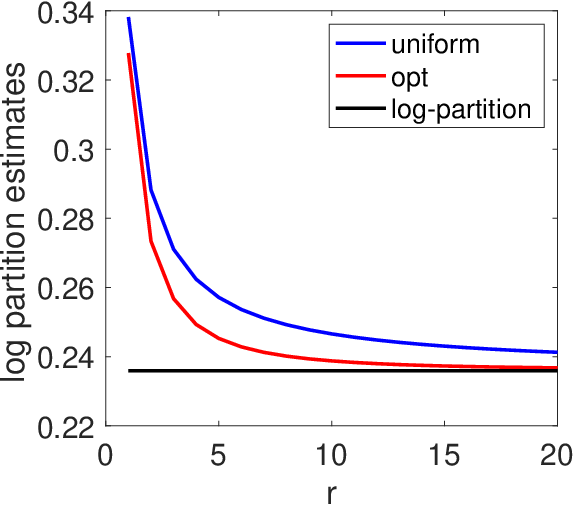
Refer to caption
Figure 4: Kernel learning for log partition estimation on the torus [0,1][0,1] with increasing order rr.

7.7 Example 2: Hypercube

We consider 𝒳={−1,1}d{\mathcal{X}}=\{-1,1\}^{d}, and φ⁡(x)=Diag(η)1/2​(x1)∈ℝd+1\displaystyle\varphi(x)=\mathop{\rm Diag}(\eta)^{1/2}{x\choose 1}\in\mathbb{R}^{d+1}, for η\eta in the simplex in ℝd+1\mathbb{R}^{d+1}. Here ℬ\mathcal{B} is exactly the set of all self-adjoint operators with diagonal equal to η\eta. To compute the entropy, we consider the set CC of positive matrices with unit diagonal, corresponding to 𝔼⁡[(x1)​(x1)⊤]{\mathbb{E}}\big[{x\choose 1}{x\choose 1}^{\top}\big].

To maximize the relative entropy with respect to the uniform distribution, we simply maximize

tr[C​(p)1/2​Diag(η)​C​(p)1/2​log⁡(C​(p)1/2​Diag(η)​C​(p)1/2)]−∑j=1d+1ηj​log⁡ηj,\mathop{\rm tr}\big[C(p)^{1/2}\mathop{\rm Diag}(\eta)C(p)^{1/2}\log(C(p)^{1/2}\mathop{\rm Diag}(\eta)C(p)^{1/2})\big]-\sum_{j=1}^{d+1}\eta_{j}\log\eta_{j},

which is a lower bound on ∑x∈{−1,1}dp⁡(x)​log⁡p⁡(x)+d​log⁡2\sum_{x\in\{-1,1\}^{d}}p(x)\log p(x)+d\log 2. Thus, we get an upperbound on the entropy

−∑x∈{−1,1}dp(x)logp(x)⩽dlog2−tr[Diag(η)1/2C(p)Diag(η)1/2log(Diag(η)1/2C(p)Diag(η)1/2)]+∑j=1d+1ηjlogηj.-\!\!\!\!\sum_{x\in\{-1,1\}^{d}}p(x)\log p(x)\leqslant d\log 2-\mathop{\rm tr}\big[\mathop{\rm Diag}(\eta)^{1/2}C(p)\mathop{\rm Diag}(\eta)^{1/2}\log(\mathop{\rm Diag}(\eta)^{1/2}C(p)\mathop{\rm Diag}(\eta)^{1/2})\big]+\sum_{j=1}^{d+1}\eta_{j}\log\eta_{j}.

With η\eta constant equal to 1/(d+1)1/(d+1), we get the upper bound: d​log⁡2−1d+1​trC⁡(p)​log⁡C⁡(p),\displaystyle d\log 2-\frac{1}{d+1}\mathop{\rm tr}C(p)\log C(p), which happens to be tight for d=1d=1.

This is to be compared to the upper-bound of [31], which is 12​log​det(C⁡(p)+13​(I000))+d2​log​π​e2.\displaystyle\frac{1}{2}\log\det\bigg(C(p)+\frac{1}{3}\bigg(\begin{array}[]{cc}I&0\\ 0&0\end{array}\bigg)\bigg)+\frac{d}{2}\log\frac{\pi e}{2}. In Figure 5, we compare these bounds on matrices CC corresponding to independent components with mean vectors uniformly distributed, showing the potential benefits of the new upperbound on entropy.

Refer to caption
Figure 5: Comparison of entropy bounds with increasing dimensions (the log-determinant bound from [31], our bound based on quantum entropy with uniform η\eta and the optimized bound). We plot the bounds for independent distributions with random probabilities for each component. We substract the true entropy and compare upper-bounds (with zero meaning that the bounds are tight).

8 Conclusion

In this paper, we presented properties of the von Neumann entropy and relative entropy of covariance operators obtained from reproducing kernel Hilbert spaces. These notions are intimately related to the usual notions of Shannon entropy and relative entropy, share many of their properties, and can be applied to any type of data where positive definite kernels can be defined. They also come with additional computational benefits, with several estimation algorithms with theoretical guarantees. We have also highlighted several properties in terms of multivariate probabilistic modeling or variational inference, but several interesting avenues for future research are worth exploring. First, exploring further approximation guarantees for log-partition function estimation can probably lead to new improved algorithms for variational inference [58] in continuous and discrete domains. Second, we could extend to Rényi entropies [36, 25] with similar developments (along the lines of Appendix A.4). Finally, the optimization with respect to the probability measure, which is at the core of log-partition estimation, can be extended to other optimization problems on probability measures, such as already done with similar tools for optimal transport [57] or optimal control [11].

Acknowledgements

The author thanks Alessandro Rudi and Loucas Pillaud-Vivien for fruitful discussions related to this work. This work was funded in part by the French government under management of Agence Nationale de la Recherche as part of the “Investissements d’avenir” program, reference ANR-19-P3IA-0001 (PRAIRIE 3IA Institute). We also acknowledge support the European Research Council (grant SEQUOIA 724063). The comments and suggestions of the anonymous reviewers were greatly appreciated.

Appendix A Proof of convexity results on operators

In this section, we provide simple direct proofs of convexity results that we use in this paper. All of these proofs are obtained from the literature, and in particular [33, 47, 46].

A.1 Joint convexity of the relative entropy

We consider a function f:ℝ+∗→ℝf:\mathbb{R}_{+}^{\ast}\to\mathbb{R}, which is operator-convex, that is, for which the function A↦f⁡(A)A\mapsto f(A) is convex as an operator-valued function, i.e., f⁡(∑i=1nλi​Ai)≼∑i=1nλi​f​(Ai)f\Big(\sum_{i=1}^{n}\lambda_{i}A_{i}\Big)\preccurlyeq\sum_{i=1}^{n}\lambda_{i}f(A_{i}). These functions can exactly be represented as: f⁡(t)=α+β⁡(t−1)+γ​(t−1)2+δ​(t−1)2t+∫0∞(t−1)2λ+t​𝑑ν​(λ),\displaystyle f(t)=\alpha+\beta(t-1)+\gamma(t-1)^{2}+\delta\frac{(t-1)^{2}}{t}+\int_{0}^{\infty}\frac{(t-1)^{2}}{\lambda+t}d\nu(\lambda), where γ,δ>0\gamma,\delta>0 and ν\nu is a positive measure with finite mass on ℝ+\mathbb{R}_{+} [33]. We have f⁡(1)=αf(1)=\alpha. The interesting case for this paper is f⁡(t)=−log⁡(t)=1−t+∫0∞(t−1)2λ+t​1(1+λ)2​𝑑λ,\displaystyle f(t)=-\log(t)=1-t+\int_{0}^{\infty}\frac{(t-1)^{2}}{\lambda+t}\frac{1}{(1+\lambda)^{2}}d\lambda, but there are others, such as, for p∈(0,1]p\in(0,1]:

−tp=−1−p⁡(t−1)+sin⁡p​ππ​∫0+∞(t−1)2λ+t​λp(1+λ)2​𝑑λ.-t^{p}=-1-p(t-1)+\frac{\sin p\pi}{\pi}\int_{0}^{+\infty}\frac{(t-1)^{2}}{\lambda+t}\frac{\lambda^{p}}{(1+\lambda)^{2}}d\lambda.

Given AA and BB two Hermitian operators, we denote by ℛA\mathcal{R}_{A} the right multiplication by AA and ℒA\mathcal{L}_{A} the left multiplication by AA. We have, since ℒB\mathcal{L}_{B} and ℛA\mathcal{R}_{A} commute, and log⁡ℒB=ℒlog⁡B\log\mathcal{L}_{B}=\mathcal{L}_{\log B} and log⁡ℛA=ℛlog⁡A\log\mathcal{R}_{A}=\mathcal{R}_{\log A}:

D(A∥B)\displaystyle D(A\|B) =\displaystyle= trA1/2​(log⁡A)​A1/2−trA1/2​(log⁡B)​A1/2=tr[(log⁡ℛA)​(A1/2)​A1/2]−tr[A1/2​(log⁡ℒB)​(A1/2)]\displaystyle\mathop{\rm tr}A^{1/2}(\log A)A^{1/2}-\mathop{\rm tr}A^{1/2}(\log B)A^{1/2}=\mathop{\rm tr}\big[(\log\mathcal{R}_{A})(A^{1/2})A^{1/2}\big]-\mathop{\rm tr}\big[A^{1/2}(\log\mathcal{L}_{B})(A^{1/2})\big]
=\displaystyle= ⟨A1/2,[log⁡ℛA−log⁡ℒB]​A1/2⟩=⟨A1/2,−log⁡[ℒB​ℛA−1]​A1/2⟩,\displaystyle\big\langle A^{1/2},\big[\log\mathcal{R}_{A}-\log\mathcal{L}_{B}\big]A^{1/2}\big\rangle=\big\langle A^{1/2},-\log\big[\mathcal{L}_{B}\mathcal{R}_{A}^{-1}\big]A^{1/2}\big\rangle,

where ⟨M,N⟩=tr(M∗​N)\langle M,N\rangle=\mathop{\rm tr}(M^{*}N) denotes the usual dot-products between operators. Following [47], we thus have:

D(A∥B)\displaystyle D(A\|B) =\displaystyle= ⟨A1/2,−log⁡[ℒB​ℛA−1]​A1/2⟩\displaystyle\big\langle A^{1/2},-\log\big[\mathcal{L}_{B}\mathcal{R}_{A}^{-1}\big]A^{1/2}\big\rangle
+∫0∞⟨(ℒBℛA−1−I)A1/2,(ℒBℛA−1+λI)−1(ℒBℛA−1−I)A1/2⟩1(1+λ)2dλ\displaystyle+\int_{0}^{\infty}\big\langle(\mathcal{L}_{B}\mathcal{R}_{A}^{-1}-I)A^{1/2},(\mathcal{L}_{B}\mathcal{R}_{A}^{-1}+\lambda I)^{-1}(\mathcal{L}_{B}\mathcal{R}_{A}^{-1}-I)A^{1/2}\big\rangle\frac{1}{(1+\lambda)^{2}}d\lambda
=\displaystyle= trA−trB+∫0∞⟨ℛA−1/2(B−A),(ℒBℛA−1+tI)−1ℛA−1/2(B−A)⟩1(1+λ)2dλ\displaystyle\mathop{\rm tr}A-\mathop{\rm tr}B+\int_{0}^{\infty}\big\langle\mathcal{R}_{A}^{-1/2}(B-A),(\mathcal{L}_{B}\mathcal{R}_{A}^{-1}+tI)^{-1}\mathcal{R}_{A}^{-1/2}(B-A)\big\rangle\frac{1}{(1+\lambda)^{2}}d\lambda
=\displaystyle= trA−trB+∫0∞⟨(B−A),(ℒB+λ​ℛA)−1​(B−A)⟩​1(1+λ)2​𝑑λ.\displaystyle\mathop{\rm tr}A-\mathop{\rm tr}B+\int_{0}^{\infty}\big\langle(B-A),(\mathcal{L}_{B}+\lambda\mathcal{R}_{A})^{-1}(B-A)\big\rangle\frac{1}{(1+\lambda)^{2}}d\lambda.

Note we can ensure the finiteness of D(A∥B)D(A\|B) as soon as B−1/2AB−1/2B^{-1/2}AB^{-1/2} is bounded. Given that the mapping (u,M)↦⟨u,M−1​u⟩(u,M)\mapsto\langle u,M^{-1}u\rangle is convex, we obtain the joint convexity of the relative entropy. It can also be shown more directly as shown below.

Proposition 12

Given positive invertible self-adjoint operators AiA_{i}, BiB_{i}, then

D(∑i=1nλiAi∥∑i=1nλiBi)⩽∑i=1nλiD(Ai∥Bi),D\Big(\sum_{i=1}^{n}\lambda_{i}A_{i}\big\|\sum_{i=1}^{n}\lambda_{i}B_{i}\Big)\leqslant\sum_{i=1}^{n}\lambda_{i}D(A_{i}\|B_{i}),

with equality if and only if for all jj such that λj>0\lambda_{j}>0,

log⁡Bj−log⁡Aj=log⁡(∑i=1nλi​Bi)−log⁡(∑i=1nλi​Ai).\log B_{j}-\log A_{j}=\log\Big(\sum_{i=1}^{n}\lambda_{i}B_{i}\Big)-\log\Big(\sum_{i=1}^{n}\lambda_{i}A_{i}\Big).

Proof Following [46, Theorem 7], we have: D(Ai∥Bi)−trAi(logA−logB)=trAi(logAi−logA+logB−logBi)=trAi−trexp(logA−logB+logBi)+B(Ai∥exp(logA−logB+logBi))D(A_{i}\|B_{i})-\mathop{\rm tr}A_{i}(\log A-\log B)=\mathop{\rm tr}A_{i}(\log A_{i}-\log A+\log B-\log B_{i})=\mathop{\rm tr}A_{i}-\mathop{\rm tr}\exp(\log A-\log B+\log B_{i})+B(A_{i}\|\exp(\log A-\log B+\log B_{i})), where B(⋅∥⋅)B(\cdot\|\cdot) is the Bregman divergence (always non-negative), defined as B(A∥B)=D(A∥B)−trA+trBB(A\|B)=D(A\|B)-\mathop{\rm tr}A+\mathop{\rm tr}B. Thus

∑i=1nλiD(Ai∥Bi)−D(A∥B)\displaystyle\sum_{i=1}^{n}\lambda_{i}D(A_{i}\|B_{i})-D(A\|B)
=\displaystyle= ∑i=1nλi[D(Ai∥Bi)−trAi(logA−logB)]\displaystyle\sum_{i=1}^{n}\lambda_{i}\Big[D(A_{i}\|B_{i})-\mathop{\rm tr}A_{i}(\log A-\log B)\Big]
=\displaystyle= trA−∑i=1nλitrexp(logA−logB+logBi)+∑i=1nλiB(Ai∥exp(logA−logB+logBi)),\displaystyle\mathop{\rm tr}A-\sum_{i=1}^{n}\lambda_{i}\mathop{\rm tr}\exp(\log A-\log B+\log B_{i})+\sum_{i=1}^{n}\lambda_{i}B(A_{i}\|\exp(\log A-\log B+\log B_{i})),

which is greater than zero since the function C↦trexp⁡(K+log⁡C)C\mapsto\mathop{\rm tr}\exp(K+\log C) is concave. There is equality if and only for all ii such that λi>0\lambda_{i}>0, Ai=exp⁡(log⁡A−log⁡B+log⁡Bi),A_{i}=\exp(\log A-\log B+\log B_{i}), because of the Bregman divergences being equal to zero.  
More generally, we get for random operators AA and BB, 𝔼[D(A∥B)]⩾D(𝔼A∥𝔼B),\displaystyle{\mathbb{E}}\big[D(A\|B)\big]\geqslant D({\mathbb{E}}A\|{\mathbb{E}}B), with equality if and only if almost surely, log⁡A−log⁡B=log⁡𝔼​A−log⁡𝔼​B\log A-\log B=\log{\mathbb{E}}A-\log{\mathbb{E}}B. Note that the concavity of the function B↦trexp⁡(M+log⁡B)B\mapsto\mathop{\rm tr}\exp(M+\log B), which is crucial in deriving concentration inequalities for matrices and operators [56], is simply obtained by partial Fenchel dualization of the relative entropy.

We can also provide more refined relationships at equality, following [39].

Proposition 13

Given positive invertible self-adjoint operators AiA_{i}, BiB_{i}, and strictly positive real numbers λi\lambda_{i} that sum to 11, then

D(∑i=1nλiAi∥∑i=1nλiBi)=∑i=1nλiD(Ai∥Bi),D\Big(\sum_{i=1}^{n}\lambda_{i}A_{i}\big\|\sum_{i=1}^{n}\lambda_{i}B_{i}\Big)=\sum_{i=1}^{n}\lambda_{i}D(A_{i}\|B_{i}),

implies that for all ii, Ai​Bi−1=A​B−1A_{i}B_{i}^{-1}=AB^{-1}, where A=∑i=1nλi​AiA=\sum_{i=1}^{n}\lambda_{i}A_{i} and B=∑i=1nλi​BiB=\sum_{i=1}^{n}\lambda_{i}B_{i}.

Proof Given the representation above, and the fact that (u,M)↦⟨u,M−1​u⟩(u,M)\mapsto\langle u,M^{-1}u\rangle is convex, we get the joint convexity of (A,B)↦D(A∥B)(A,B)\mapsto D(A\|B) is convex. In order to study the equality sign, we can use the lemma below, and for each λ>0\lambda>0, [ℒBi+λ​ℛAi]−1​(Bi−Ai)=[ℒB+λ​ℛA]−1​(B−A)\big[\mathcal{L}_{B_{i}}+\lambda\mathcal{R}_{A_{i}}\big]^{-1}(B_{i}-A_{i})=\big[\mathcal{L}_{B}+\lambda\mathcal{R}_{A}\big]^{-1}(B-A). By letting λ\lambda go to zero, we get the result.

Note that following [39], we can also consider that

(ℒBi+λ​ℛAi)−1​(Bi−Ai)=(ℒBi​ℛAi−1+λ​I)−1​[ℒBi​ℛAi−1−I]​I​ is independent of ​i,(\mathcal{L}_{B_{i}}+\lambda\mathcal{R}_{A_{i}})^{-1}(B_{i}-A_{i})=(\mathcal{L}_{B_{i}}\mathcal{R}_{A_{i}}^{-1}+\lambda I)^{-1}\big[\mathcal{L}_{B_{i}}\mathcal{R}_{A_{i}}^{-1}-I\big]I\mbox{ is independent of }i,

and is equal to (ℒB​ℛA−1+λ​I)−1​[ℒB​ℛA−1−I]​I(\mathcal{L}_{B}\mathcal{R}_{A}^{-1}+\lambda I)^{-1}\big[\mathcal{L}_{B}\mathcal{R}_{A}^{-1}-I\big]I. Thus by using representations of a function f:ℝ+→ℝf:\mathbb{R}_{+}\to\mathbb{R} as f⁡(t)=(t−1)​∫0∞d​ν​(λ)t+λ\displaystyle f(t)=(t-1)\int_{0}^{\infty}\frac{d\nu(\lambda)}{t+\lambda} for a certain signed measure d​νd\nu, we can deduce that f⁡[ℒBi​ℛAi−1]​I​ is independent of ​i,f\big[\mathcal{L}_{B_{i}}\mathcal{R}_{A_{i}}^{-1}\big]I\mbox{ is independent of }i, and equal to f⁡[ℒB​ℛA−1]​If\big[\mathcal{L}_{B}\mathcal{R}_{A}^{-1}\big]I. For example. with f⁡(t)=log⁡tf(t)=\log t, we get log⁡Bi−log⁡Ai\log B_{i}-\log A_{i} independent of ii. For example. with f⁡(t)=t−1f(t)=t-1, we get Bi​Ai−1B_{i}A_{i}^{-1} independent of ii. For f⁡(t)=tzf(t)=t^{z}, Biz​Ai−zB_{i}^{z}A_{i}^{-z} independent of ii, for any complex zz.  

Lemma 1

If M1,…,MnM_{1},\dots,M_{n} are invertible and all λi\lambda_{i} are strictly positive and sum to 11, then

∑i=1nλi​ui⊤​Mi−1​ui=(∑i=1nλi​ui)​(∑i=1nλi​Mi)−1​(∑i=1nλi​ui)\sum_{i=1}^{n}\lambda_{i}u_{i}^{\top}M_{i}^{-1}u_{i}=\Big(\sum_{i=1}^{n}\lambda_{i}u_{i}\Big)\Big(\sum_{i=1}^{n}\lambda_{i}M_{i}\Big)^{-1}\Big(\sum_{i=1}^{n}\lambda_{i}u_{i}\Big)

if and only if Mi−1​uiM_{i}^{-1}u_{i} is independent of ii, and equal to M−1​uM^{-1}u where M=∑i=1nλi​MiM=\sum_{i=1}^{n}\lambda_{i}M_{i} and u=∑i=1nλi​uiu=\sum_{i=1}^{n}\lambda_{i}u_{i}.

Proof We consider the function f⁡(u,M)=u⊤​M−1​uf(u,M)=u^{\top}M^{-1}u, with Taylor expansion

f⁡(u+δ,M+Δ)=f⁡(u,M)+2​δ⊤​M−1​u−u⊤​M−1​Δ​M−1​u+2​(δ−Δ​M−1​u)⊤​M−1​(δ−Δ​M−1​u)+O⁡(‖Δ‖3+‖δ‖3).f(u+\delta,M+\Delta)=f(u,M)+2\delta^{\top}M^{-1}u-u^{\top}M^{-1}\Delta M^{-1}u+2(\delta-\Delta M^{-1}u)^{\top}M^{-1}(\delta-\Delta M^{-1}u)+O(\|\Delta\|^{3}+\|\delta\|^{3}).

We now use the following result on the remainder in Jensen’s inequality (which itself is a direct consequence of the Taylor expansion with integral remainder taken at XX, while expanded at 𝔼​X{\mathbb{E}}X):

𝔼​f​(X)−f⁡(𝔼​X)=∫01𝔼⁡[(X−𝔼​X)⊤​f′′​(t​X+(1−t)​𝔼​X)​(X−𝔼​X)]​𝑑t.{\mathbb{E}}f(X)-f({\mathbb{E}}X)=\int_{0}^{1}{\mathbb{E}}\Big[(X-{\mathbb{E}}X)^{\top}f^{\prime\prime}(tX+(1-t){\mathbb{E}}X)(X-{\mathbb{E}}X)\Big]dt. (15)

In our particular situation, by the invertibility assumption, the matrix MM is invertible almost surely, and having equality in Jensen’s inequality imposes to have (X−𝔼​X)⊤​f′′​(t​X+(1−t)​𝔼​X)​(X−𝔼​X)=0(X-{\mathbb{E}}X)^{\top}f^{\prime\prime}(tX+(1-t){\mathbb{E}}X)(X-{\mathbb{E}}X)=0 almost surely in tt and XX. Thus, at t=0t=0 and X=(ui,Mi)X=(u_{i},M_{i}), we get: ui−u−(Mi−M)​M−1​u=0u_{i}-u-(M_{i}-M)M^{-1}u=0, which is exactly Mi−1​ui=M−1​uM_{i}^{-1}u_{i}=M^{-1}u.  

A.2 Monotonicity of the relative entropy

Proposition 14

Given operators CiC_{i}, i=1,…,ni=1,\dots,n, such that ∑i=1nCi∗​Ci=I\sum_{i=1}^{n}C_{i}^{\ast}C_{i}=I, then

D(∑i=1nCiACi∗∥∑i=1nCiBCi∗)⩽D(A∥B).D\Big(\sum_{i=1}^{n}C_{i}AC_{i}^{\ast}\Big\|\sum_{i=1}^{n}C_{i}BC_{i}^{\ast}\Big)\leqslant D(A\|B).

Proof We have, with ω=exp⁡(2​i​π/n)\omega=\exp(2i\pi/n), using the joint convexity of the relative entropy and the expression 1n​∑k=1nωk⁡(i−j)=1i=j\frac{1}{n}\sum_{k=1}^{n}\omega^{k(i-j)}=1_{i=j}:

D(∑i=1nCiACi∗∥∑i=1nCiBCi∗)\displaystyle D\Big(\sum_{i=1}^{n}C_{i}AC_{i}^{\ast}\Big\|\sum_{i=1}^{n}C_{i}BC_{i}^{\ast}\Big) ⩽\displaystyle\leqslant ∑i=1nD(CiACi∗∥CiBCi∗)=D(∑i=1n(eiei⊤)⊗EiAEi∗∥∑i=1n(eiei⊤)⊗CiBCi∗)\displaystyle\sum_{i=1}^{n}D(C_{i}AC_{i}^{\ast}\|C_{i}BC_{i}^{\ast})=D\Big(\sum_{i=1}^{n}(e_{i}e_{i}^{\top})\otimes E_{i}AE_{i}^{\ast}\Big\|\sum_{i=1}^{n}(e_{i}e_{i}^{\top})\otimes C_{i}BC_{i}^{\ast}\Big)
=\displaystyle= D(1n∑k=1nωk⁡(i−j)∑i,j=1n(eiej⊤)⊗CiACj∗∥1n∑k=1nωk⁡(i−j)∑i,j=1n(eiej⊤)⊗CiBCj∗).\displaystyle D\Big(\frac{1}{n}\sum_{k=1}^{n}\omega^{k(i-j)}\sum_{i,j=1}^{n}(e_{i}e_{j}^{\top})\otimes C_{i}AC_{j}^{\ast}\Big\|\frac{1}{n}\sum_{k=1}^{n}\omega^{k(i-j)}\sum_{i,j=1}^{n}(e_{i}e_{j}^{\top})\otimes C_{i}BC_{j}^{\ast}\Big).

Consider the matrices MM and NN defined by blocks Mi​j=Ci​A​Cj∗M_{ij}=C_{i}AC_{j}^{\ast} and Ni​j=Ci​B​Cj∗N_{ij}=C_{i}BC_{j}^{\ast}, as well as, the matrix UkU_{k} defined by blocks (Uk)i​j=1i=j​ωk​i​I(U_{k})_{ij}=1_{i=j}\omega^{ki}I, we get from the equation above:

D(∑i=1nCiACi∗∥∑i=1nCiBCi∗)\displaystyle D\Big(\sum_{i=1}^{n}C_{i}AC_{i}^{\ast}\Big\|\sum_{i=1}^{n}C_{i}BC_{i}^{\ast}\Big) ⩽\displaystyle\leqslant D(1n∑k=1nUkMUk∗∥1n∑k=1nUkNUk∗)\displaystyle D\Big(\frac{1}{n}\sum_{k=1}^{n}U_{k}MU_{k}^{\ast}\Big\|\frac{1}{n}\sum_{k=1}^{n}U_{k}NU_{k}^{\ast}\Big)
⩽\displaystyle\leqslant 1n∑k=1nD(UkMUk∗∥UkMUk∗)=D(M∥N)\displaystyle\frac{1}{n}\sum_{k=1}^{n}D\Big(U_{k}MU_{k}^{\ast}\Big\|U_{k}MU_{k}^{\ast}\Big)=D(M\|N)

because each UkU_{k} is unitary. Moreover, we can write M=V​A​V∗M=VAV^{*} and N=V​A​V∗N=VAV^{\ast}, with a an operator VV defined by a column of blocks CiC_{i}, i=1,…,ni=1,\dots,n, so that V∗​V=∑i=1nCi∗​Ci=IV^{*}V=\sum_{i=1}^{n}C_{i}^{\ast}C_{i}=I. Thus D(M∥N)=D(A∥B)D(M\|N)=D(A\|B), which shows the desired bound.

Using propositions above, there is is equality if and only: log⁡(Ci​B​Ci∗)−log⁡(Ci​A​Ci∗)\log(C_{i}BC_{i}^{\ast})-\log(C_{i}AC_{i}^{\ast}) independent of ii and OPENlog⁡[Uk​N​Uk∗]−log⁡[Uk​M​Uk∗]=Uk​(log⁡N−log⁡M))​Uk∗\log[U_{k}NU_{k}^{\ast}\ ]-\log[U_{k}MU_{k}^{\ast}]=U_{k}(\log N-\log M)\big)U_{k}^{\ast} independent of kk, that is log⁡N−log⁡M\log N-\log M block diagonal. Overall, we get equality if log⁡N−log⁡M\log N-\log M is block diagonal with equal blocks.

We can also obtain necessary conditions for equality, that is, (Ci​B​Ci∗)​(Ci​A​Ci∗)−1(C_{i}BC_{i}^{\ast})(C_{i}AC_{i}^{\ast})^{-1} independent of ii, and Uk​N​Uk∗​[Uk​N​Uk∗]−1=Uk​N​M−1​Uk∗U_{k}NU_{k}^{\ast}[U_{k}NU_{k}^{\ast}]^{-1}=U_{k}NM^{-1}U_{k}^{\ast} independent of kk, that is, N​M−1NM^{-1} block-diagonal with equal blocks.


This extends to a random operator CC, such that 𝔼⁡[C∗​C]=I{\mathbb{E}}\big[C^{\ast}C\big]=I, for which we get:

D(𝔼[CAC∗]∥𝔼[CBC∗])⩽D(A∥B).D\Big({\mathbb{E}}\big[CAC^{\ast}\big]\,\big\|\,{\mathbb{E}}\big[CBC^{\ast}\big]\Big)\leqslant D(A\|B).

A particular example is obtained from nn Hermitian positive operators D1,…,DnD_{1},\dots,D_{n} such that ∑i=1nDi=I\sum_{i=1}^{n}D_{i}=I, and we get, with μi=tr(Di​A)\mu_{i}=\mathop{\rm tr}(D_{i}A) and νi=tr(Di​B)\nu_{i}=\mathop{\rm tr}(D_{i}B):

∑i=1nμilogμiνi⩽D(A∥B).\sum_{i=1}^{n}\mu_{i}\log\frac{\mu_{i}}{\nu_{i}}\leqslant D(A\|B).

This corresponds to, if Di=∑kλi​k​ui​k⊗ui​kD_{i}=\sum_{k}\lambda_{ik}u_{ik}\otimes u_{ik}, to Ci​k=λi​k1/2​ei​ui​k∗C_{ik}=\lambda_{ik}^{1/2}e_{i}u_{ik}^{\ast}, so that

∑i,kEi​A​Ei∗=∑i,kλi​k​ei​ui​k∗​M​ui​k​ei∗=∑i=1n(trA​Di)​ei​ei∗.\sum_{i,k}E_{i}AE_{i}^{\ast}=\sum_{i,k}\lambda_{ik}e_{i}u_{ik}^{\ast}Mu_{ik}e_{i}^{\ast}=\sum_{i=1}^{n}(\mathop{\rm tr}AD_{i})e_{i}e_{i}^{\ast}.

A.3 Concavity of relative entropy

In this section, we consider two positive self-adjoint operators, MM and NN such that M≼α​NM\preccurlyeq\alpha N for some α\alpha. We consider the function:

f:Λ→D(Λ1/2MΛ1/2∥Λ1/2NΛ1/2).f:\Lambda\to D(\Lambda^{1/2}M\Lambda^{1/2}\|\Lambda^{1/2}N\Lambda^{1/2}).

It happens to be convex in (M,N)(M,N). It is also concave in Λ\Lambda in the set of positive bounded operators. This is due to the representation, valid for invertible operators:

f⁡(Λ)−trM​Λ+trN​Λ\displaystyle f(\Lambda)-\mathop{\rm tr}M\Lambda+\mathop{\rm tr}N\Lambda
=\displaystyle= ∫0∞⟨Λ1/2​(N−M)​Λ1/2,(ℒΛ1/2​N​Λ1/2+λ​ℛΛ1/2​M​Λ1/2)−1​Λ1/2​(N−M)​Λ1/2⟩​1(1+λ)2​𝑑λ\displaystyle\int_{0}^{\infty}\big\langle\Lambda^{1/2}(N-M)\Lambda^{1/2},(\mathcal{L}_{\Lambda^{1/2}N\Lambda^{1/2}}+\lambda\mathcal{R}_{\Lambda^{1/2}M\Lambda^{1/2}})^{-1}\Lambda^{1/2}(N-M)\Lambda^{1/2}\big\rangle\frac{1}{(1+\lambda)^{2}}d\lambda
=\displaystyle= ∫0∞⟨(N−M),(ℒN​ℛΛ−1+λ​ℒΛ−1​ℛM)−1​(N−M)⟩​1(1+λ)2​𝑑λ.\displaystyle\int_{0}^{\infty}\big\langle(N-M),(\mathcal{L}_{N}\mathcal{R}_{\Lambda}^{-1}+\lambda\mathcal{L}_{\Lambda}^{-1}\mathcal{R}_{M})^{-1}(N-M)\big\rangle\frac{1}{(1+\lambda)^{2}}d\lambda.

Since the mapping (A,B)↦(A−1+B−1)−1=B−B​(A+B)−1​B(A,B)\mapsto(A^{-1}+B^{-1})^{-1}=B-B(A+B)^{-1}B is matrix-concave [1, Corollary 1.1], we get the desired concavity.

A.4 Extension to other divergences

As mentioned in [47], both the joint convexity and the monotonicity of the relative entropy D(A∥B)D(A\|B) in Prop. 12 and Prop. 14 can be extended to most operator-convex functions on ℝ+∗\mathbb{R}_{+}^{\ast}, and

Df(A∥B)=⟨A1/2,f[ℒBℛA−1]A1/2⟩,D_{f}(A\|B)=\big\langle A^{1/2},f\big[\mathcal{L}_{B}\mathcal{R}_{A}^{-1}\big]A^{1/2}\big\rangle,

with the relative entropy being D−logD_{\rm-\log}. Among other interesting cases, we have:

  • •

    f⁡(t)=(t−1)2\displaystyle f(t)=(t-1)^{2}, with Df(A∥B)=tr[(B−A)2A−1]D_{f}(A\|B)=\mathop{\rm tr}\big[(B-A)^{2}A^{-1}\big].

  • •

    f⁡(t)=(t−1)2t\displaystyle f(t)=\frac{(t-1)^{2}}{t}, with Df(A∥B)=tr[(B−A)2B−1]D_{f}(A\|B)=\mathop{\rm tr}\big[(B-A)^{2}B^{-1}\big].

  • •

    f⁡(t)=(t−1)21+t\displaystyle f(t)=\frac{(t-1)^{2}}{1+t}, with Df(A∥B)=⟨A1/2,(ℒB+ℛA)−1A1/2⟩D_{f}(A\|B)=\langle A^{1/2},(\mathcal{L}_{B}+\mathcal{R}_{A})^{-1}A^{1/2}\rangle.

  • •

    f⁡(t)=1−t\displaystyle f(t)=1-\sqrt{t}, with Df(A∥B)=tr(A)−⟨A1/2,[ℒBℛA−1]1/2A1/2⟩D_{f}(A\|B)=\mathop{\rm tr}(A)-\big\langle A^{1/2},[\mathcal{L}_{B}\mathcal{R}_{A}^{-1}\big]^{1/2}A^{1/2}\big\rangle.

Specialized to covariance operators, we have, with A=ΣpA=\Sigma_{p} and B=ΣqB=\Sigma_{q}, and following the same reasoning as in the proof of Prop. 4:

Df(Σp∥Σq)\displaystyle D_{f}(\Sigma_{p}\|\Sigma_{q}) ⩽\displaystyle\leqslant ∫𝒳Df(φ(x)φ(x)∗∥d​qd​p(x)φ(x)φ(x)∗)dp(x)\displaystyle\int_{\mathcal{X}}D_{f}\Big(\varphi(x)\varphi(x)^{\ast}\Big\|\frac{dq}{dp}(x)\varphi(x)\varphi(x)^{\ast}\Big)dp(x)
=\displaystyle= ∫𝒳f(d​qd​p(x))dp(x)=Df(p∥q),\displaystyle\int_{\mathcal{X}}f\Big(\frac{dq}{dp}(x)\Big)dp(x)=D_{f}(p\|q),

which is the reverse ff-divergence associated with the function ff [19, 55]. We thus immediately get lower bounds on:

  • •

    the square Hellinger distance Df(p∥q)=∫𝒳[1−(d​qd​p(x))1/2]dp(x)=12∫𝒳[(d​qd​τ(x))1/2−(d​pd​τ(x))1/2]2dτ(x)\displaystyle D_{f}(p\|q)=\int_{\mathcal{X}}\Big[1-\Big(\frac{dq}{dp}(x)\Big)^{1/2}\Big]dp(x)=\frac{1}{2}\int_{\mathcal{X}}\Big[\Big(\frac{dq}{d\tau}(x)\Big)^{1/2}-\Big(\frac{dp}{d\tau}(x)\Big)^{1/2}\Big]^{2}d\tau(x) for f⁡(t)=1−tf(t)=1-\sqrt{t},

  • •

    the reverse Pearson χ2\chi^{2}-divergence Df(p∥q)=∫𝒳[1−d​qd​p(x)]2dp(x)=12∫𝒳[d​qd​τ(x)−d​pd​τ(x)]2d​τ​(x)d​p/d​τ​(x)\displaystyle D_{f}(p\|q)=\int_{\mathcal{X}}\Big[1-\frac{dq}{dp}(x)\Big]^{2}dp(x)=\frac{1}{2}\int_{\mathcal{X}}\Big[\frac{dq}{d\tau}(x)-\frac{dp}{d\tau}(x)\Big]^{2}\frac{d\tau(x)}{dp/d\tau(x)} for f⁡(t)=(t−1)2f(t)=(t-1)^{2},

  • •

    the Pearson χ2\chi^{2}-divergence Df(p∥q)=∫𝒳[1−d​qd​p(x)]2d​p​(x)d​q/d​p​(x)=12∫𝒳[d​qd​τ(x)−d​pd​τ(x)]2d​τ​(x)d​q/d​τ​(x)\displaystyle D_{f}(p\|q)=\int_{\mathcal{X}}\Big[1-\frac{dq}{dp}(x)\Big]^{2}\frac{dp(x)}{dq/dp(x)}=\frac{1}{2}\int_{\mathcal{X}}\Big[\frac{dq}{d\tau}(x)-\frac{dp}{d\tau}(x)\Big]^{2}\frac{d\tau(x)}{dq/d\tau(x)} for f⁡(t)=(t−1)2t\displaystyle f(t)=\frac{(t-1)^{2}}{t},

  • •

    the Vincze-Le Cam distance Df(p∥q)=∫𝒳[1−d​qd​p(x)]2d​p​(x)1+d​q/d​p​(x)\displaystyle D_{f}(p\|q)=\int_{\mathcal{X}}\Big[1-\frac{dq}{dp}(x)\Big]^{2}\frac{dp(x)}{1+dq/dp(x)}
    equal to 12​∫𝒳[d​qd​τ​(x)−d​pd​τ​(x)]2​d​τ​(x)d​q/d​τ​(x)+d​p/d​τ​(x)\displaystyle\frac{1}{2}\int_{\mathcal{X}}\Big[\frac{dq}{d\tau}(x)-\frac{dp}{d\tau}(x)\Big]^{2}\frac{d\tau(x)}{dq/d\tau(x)+dp/d\tau(x)} for f⁡(t)=(t−1)21+t\displaystyle f(t)=\frac{(t-1)^{2}}{1+t}.

Appendix B Proof of lower bound (Prop. 5)

Proof Starting from p~​(y)=∫𝒳h⁡(x,y)​𝑑p​(x)\tilde{p}(y)=\int_{\mathcal{X}}h(x,y)dp(x) and q~​(y)=∫𝒳h⁡(x,y)​𝑑q​(x)\tilde{q}(y)=\int_{\mathcal{X}}h(x,y)dq(x), we can provide an exact expression in the usual data processing inequality for the regular KL divergence [18], with two joint distributions p¯​(x,y)=p⁡(x)​h​(x,y)\bar{p}(x,y)=p(x)h(x,y) and q¯​(x,y)=q⁡(x)​h​(x,y)\bar{q}(x,y)=q(x)h(x,y), so that, with f⁡(u)=u​log⁡uf(u)=u\log u:

D(p∥q)\displaystyle D(p\|q) =\displaystyle= D(p¯∥q¯)=∫𝒳∫𝒳q¯(x,y)f(p¯​(x,y)q¯​(x,y))dτ(x)dτ(y)\displaystyle D(\bar{p}\|\bar{q})=\int_{{\mathcal{X}}}\int_{\mathcal{X}}\bar{q}(x,y)f\Big(\frac{\bar{p}(x,y)}{\bar{q}(x,y)}\Big)d\tau(x)d\tau(y)
⩾\displaystyle\geqslant ∫𝒳q~​(y)​f​(∫𝒳q¯​(x|y)​p¯​(x,y)q¯​(x,y)​𝑑τ​(x))​𝑑τ​(y)​ by Jensen’s inequality,\displaystyle\int_{\mathcal{X}}\tilde{q}(y)f\Big(\int_{\mathcal{X}}\bar{q}(x|y)\frac{\bar{p}(x,y)}{\bar{q}(x,y)}d\tau(x)\Big)d\tau(y)\mbox{ by Jensen's inequality},
=\displaystyle= ∫𝒳q~(y)f(p~​(y)q~​(y))dτ(y)=D(p~∥q~).\displaystyle\int_{\mathcal{X}}\tilde{q}(y)f\Big(\ \frac{\tilde{p}(y)}{\tilde{q}(y)}\Big)d\tau(y)=D(\tilde{p}\|\tilde{q}).

Using Eq. (15), we thus get

D(p∥q)−D(p~∥q~)\displaystyle D(p\|q)-D(\tilde{p}\|\tilde{q}) =\displaystyle= ∫𝒳∫𝒳q~​(y)​h​(x,y)​(p⁡(x)q⁡(x)−p~​(y)q~​(y))2​(∫01d​tt​p⁡(x)q⁡(x)+(1−t)​p~​(y)q~​(y))​𝑑τ​(x)​𝑑τ​(y).\displaystyle\int_{\mathcal{X}}\int_{\mathcal{X}}\tilde{q}(y)h(x,y)\Big(\frac{p(x)}{q(x)}-\frac{\tilde{p}(y)}{\tilde{q}(y)}\Big)^{2}\Big(\int_{0}^{1}\frac{dt}{t\frac{p(x)}{q(x)}+(1-t)\frac{\tilde{p}(y)}{\tilde{q}(y)}}\Big)d\tau(x)d\tau(y).

Since for all x∈𝒳x\in{\mathcal{X}}, t​p⁡(x)q⁡(x)+(1−t)​p~​(y)q~​(y)⩾infx∈𝒳p⁡(x)q⁡(x)t\frac{p(x)}{q(x)}+(1-t)\frac{\tilde{p}(y)}{\tilde{q}(y)}\geqslant\inf_{x\in{\mathcal{X}}}\frac{p(x)}{q(x)}, we can then bound as

D(p∥q)−D(p~∥q~)\displaystyle D(p\|q)-D(\tilde{p}\|\tilde{q}) ⩽\displaystyle\leqslant supx∈𝒳q⁡(x)p⁡(x)​∫𝒳∫𝒴q~​(y)​h​(x,y)​(p⁡(x)q⁡(x)−p~​(y)q~​(y))2​𝑑τ​(x)​𝑑τ​(y)\displaystyle\sup_{x\in{\mathcal{X}}}\frac{q(x)}{p(x)}\int_{\mathcal{X}}\int_{\mathcal{Y}}\tilde{q}(y)h(x,y)\Big(\frac{p(x)}{q(x)}-\frac{\tilde{p}(y)}{\tilde{q}(y)}\Big)^{2}d\tau(x)d\tau(y)
=\displaystyle= supx∈𝒳q⁡(x)p⁡(x)​∫𝒳∫𝒳q~​(y)​h​(x,y)​(p⁡(x)q⁡(x)−p⁡(y)q⁡(y)+p⁡(y)q⁡(y)−p~​(y)q~​(y))2​𝑑τ​(x)​𝑑τ​(y)\displaystyle\sup_{x\in{\mathcal{X}}}\frac{q(x)}{p(x)}\int_{\mathcal{X}}\int_{\mathcal{X}}\tilde{q}(y)h(x,y)\Big(\frac{p(x)}{q(x)}-\frac{p(y)}{q(y)}+\frac{p(y)}{q(y)}-\frac{\tilde{p}(y)}{\tilde{q}(y)}\Big)^{2}d\tau(x)d\tau(y)
⩽\displaystyle\leqslant 2​supx∈𝒳q⁡(x)p⁡(x)​∫𝒳∫𝒳q~​(y)​h​(x,y)​(p⁡(x)q⁡(x)−p⁡(y)q⁡(y))2​𝑑τ​(x)​𝑑τ​(y)\displaystyle 2\sup_{x\in{\mathcal{X}}}\frac{q(x)}{p(x)}\int_{\mathcal{X}}\int_{\mathcal{X}}\tilde{q}(y)h(x,y)\Big(\frac{p(x)}{q(x)}-\frac{p(y)}{q(y)}\Big)^{2}d\tau(x)d\tau(y)
+2supx∈𝒳q⁡(x)p⁡(x)∫𝒳q~(y)(p⁡(y)q⁡(y)−p~​(y)q~​(y))2dτ(y).\displaystyle+2\sup_{x\in{\mathcal{X}}}\frac{q(x)}{p(x)}\int_{\mathcal{X}}\tilde{q}(y)\Big(\frac{p(y)}{q(y)}-\frac{\tilde{p}(y)}{\tilde{q}(y)}\Big)^{2}d\tau(y).

We assume Lipschitz-continuity for pp and qq in the following form: for all x,yx,y, |q⁡(x)q⁡(y)−1|⩽d⁡(x,y)​Cq\big|\frac{q(x)}{q(y)}-1\big|\leqslant d(x,y)C_{q}, |p⁡(x)p⁡(y)−1|⩽d⁡(x,y)​Cp\big|\frac{p(x)}{p(y)}-1\big|\leqslant d(x,y)C_{p}, and |p⁡(y)q⁡(y)−p⁡(x)q⁡(x)|⩽d⁡(x,y)​Cp/q\big|\frac{p(y)}{q(y)}-\frac{p(x)}{q(x)}\big|\leqslant d(x,y)C_{p/q} for some distance dd on 𝒳{\mathcal{X}}. Then the first term in the bound above is less than 2​Cp/q2​supx∈𝒳q⁡(x)p⁡(x)​supx∈𝒳∫𝒳h⁡(x,y)​d​(x,y)2​𝑑τ​(y)\displaystyle 2C_{p/q}^{2}\sup_{x\in{\mathcal{X}}}\frac{q(x)}{p(x)}\sup_{x\in{\mathcal{X}}}\int_{\mathcal{X}}h(x,y)d(x,y)^{2}d\tau(y). For the second term, we write:

|p⁡(y)q⁡(y)−p~​(y)q~​(y)|\displaystyle\Big|\frac{p(y)}{q(y)}-\frac{\tilde{p}(y)}{\tilde{q}(y)}\Big| ⩽\displaystyle\leqslant p⁡(y)|q~​(y)−q⁡(y)|+q⁡(y)​|p~​(y)−p⁡(y)|q⁡(y)​q~​(y)\displaystyle\frac{p(y)|\tilde{q}(y)-q(y)|+q(y)|\tilde{p}(y)-p(y)|}{q(y)\tilde{q}(y)}
⩽\displaystyle\leqslant p⁡(y)​∫𝒳|q⁡(y)−q⁡(y)|​h​(x,y)​𝑑τ​(x)+q⁡(y)​∫𝒳|p⁡(y)−p⁡(y)|​h​(x,y)​𝑑τ​(x)q⁡(y)​q~​(y)\displaystyle\frac{p(y)\int_{\mathcal{X}}|q(y)-q(y)|h(x,y)d\tau(x)+q(y)\int_{\mathcal{X}}|p(y)-p(y)|h(x,y)d\tau(x)}{q(y)\tilde{q}(y)}
⩽\displaystyle\leqslant Cq​p​(y)​q​(y)​∫𝒳d⁡(x,y)​h​(x,y)​𝑑τ​(x)+Cp​q​(y)​p​(y)​∫𝒳d⁡(x,y)​h​(x,y)​𝑑τ​(x)q⁡(y)​q~​(y)\displaystyle\frac{C_{q}p(y)q(y)\int_{\mathcal{X}}d(x,y)h(x,y)d\tau(x)+C_{p}q(y)p(y)\int_{\mathcal{X}}d(x,y)h(x,y)d\tau(x)}{q(y)\tilde{q}(y)}
⩽\displaystyle\leqslant (Cp+Cq)​p​(y)q~​(y)​∫𝒳d⁡(x,y)​h​(x,y)​𝑑τ​(x)⩽(Cp+Cq)​p​(y)q~​(y)​(∫𝒳d​(x,y)2​h​(x,y)​𝑑τ​(x))1/2.\displaystyle\frac{(C_{p}+C_{q})p(y)}{\tilde{q}(y)}\int_{\mathcal{X}}d(x,y)h(x,y)d\tau(x)\leqslant\frac{(C_{p}+C_{q})p(y)}{\tilde{q}(y)}\bigg(\int_{\mathcal{X}}d(x,y)^{2}h(x,y)d\tau(x)\bigg)^{1/2}.

Moreover

∫𝒳p​(y)2q~​(y)​𝑑τ​(y)\displaystyle\int_{\mathcal{X}}\frac{p(y)^{2}}{\tilde{q}(y)}d\tau(y) ⩽\displaystyle\leqslant supx∈𝒳p⁡(x)q⁡(x)​∫𝒳2​p~​(y)2+2​(p~​(y)−p⁡(y))2p~​(y)​𝑑τ​(y)\displaystyle\sup_{x\in{\mathcal{X}}}\frac{p(x)}{q(x)}\int_{\mathcal{X}}\frac{2\tilde{p}(y)^{2}+2(\tilde{p}(y)-p(y))^{2}}{\tilde{p}(y)}d\tau(y)
⩽\displaystyle\leqslant 2​supx∈𝒳p⁡(x)q⁡(x)​(1+∫𝒳(p~​(y)−p​(y))2p~​(y)​𝑑τ​(y))⩽2​supx∈𝒳p⁡(x)q⁡(x)​(1+Cp2​diam​(𝒳)2).\displaystyle 2\sup_{x\in{\mathcal{X}}}\frac{p(x)}{q(x)}\Big(1+\int_{\mathcal{X}}\frac{(\tilde{p}(y)-p(y))^{2}}{\tilde{p}(y)}d\tau(y)\Big)\leqslant 2\sup_{x\in{\mathcal{X}}}\frac{p(x)}{q(x)}(1+C_{p}^{2}{\rm diam}({\mathcal{X}})^{2}).

Overall, we get D(p∥q)−D(p~∥q~)⩽E(p,q)×supx∈𝒳∫h(x,y)d(x,y)2dy,\displaystyle D(p\|q)-D(\tilde{p}\|\tilde{q})\leqslant E(p,q)\times\sup_{x\in{\mathcal{X}}}\int h(x,y)d(x,y)^{2}dy, with E⁡(p,q)=2​Cp/q2​supx∈𝒳q⁡(x)p⁡(x)+4​supx∈𝒳q⁡(x)p⁡(x)​(Cp+Cq)2​supx∈𝒳p⁡(x)q⁡(x)​(1+Cp2​diam​(𝒳)2)E(p,q)=2C_{p/q}^{2}\sup_{x\in{\mathcal{X}}}\frac{q(x)}{p(x)}+4\sup_{x\in{\mathcal{X}}}\frac{q(x)}{p(x)}(C_{p}+C_{q})^{2}\sup_{x\in{\mathcal{X}}}\frac{p(x)}{q(x)}(1+C_{p}^{2}{\rm diam}({\mathcal{X}})^{2}).  

Appendix C Convergence of estimation algorithms

In this Appendix, we give convergence proofs for the estimation algorithms from Section 5, starting with concentration inequalities for operators and bounds on degrees of freedom.

C.1 Concentration of sums of random self-adjoint operators

We recall in this Appendix classical results on the concentation of covariance operators.

Lemma 2 (Concentration of covariance operators [45, 56])

Let φ\varphi be mapping φ:𝒳→ℋ\varphi:{\mathcal{X}}\to{\mathcal{H}} between a measurable space 𝒳{\mathcal{X}} and a separable Hilbert space ℋ{\mathcal{H}}, such that for all x∈𝒳x\in{\mathcal{X}}, ‖φ⁡(x)‖⩽R\|\varphi(x)\|\leqslant R. Given Σp=∫𝒳φ⁡(x)​φ​(x)∗​𝑑p​(x)\Sigma_{p}=\displaystyle\int_{\mathcal{X}}\varphi(x)\varphi(x)^{\ast}dp(x), assume that λmax​(Σp)⩽μ\lambda_{\max}(\Sigma_{p})\leqslant\mu. Given x1,…,xn∈𝒳x_{1},\dots,x_{n}\in{\mathcal{X}} nn i.i.d. samples from pp, then, for all u>0u>0,

ℙ⁡(λmax​(Σp−1n​∑i=1nφ⁡(xi)⊗φ⁡(xi))>u)⩽trΣpμ​(1+3​μ2u4​n2​(R2+u3)2)​exp⁡(−n​u22​μ​(R2+u3)).{\mathbb{P}}\bigg(\lambda_{\max}\Big(\Sigma_{p}-\frac{1}{n}\sum_{i=1}^{n}\varphi(x_{i})\otimes\varphi(x_{i})\Big)>u\bigg)\leqslant\frac{\mathop{\rm tr}\Sigma_{p}}{\mu}\Big(1+\frac{3\mu^{2}}{u^{4}n^{2}}\big(R^{2}+\frac{u}{3}\big)^{2}\Big)\exp\Big(-\frac{nu^{2}}{2\mu(R^{2}+\frac{u}{3})}\Big).

We will apply the lemma above to φ~(x)=(Σp+λI)−1/2φ(x)\tilde{\varphi}(x)=(\Sigma_{p}+\lambda I)^{-1/2}\varphi(x), with Σp=∫𝒳φ⁡(x)⊗φ⁡(x)​𝑑p​(x)\displaystyle\Sigma_{p}=\int_{\mathcal{X}}\varphi(x)\otimes\varphi(x)dp(x) and Σ^=1n​∑i=1nφ⁡(xi)⊗φ⁡(xi)\displaystyle\hat{\Sigma}=\frac{1}{n}\sum_{i=1}^{n}\varphi(x_{i})\otimes\varphi(x_{i}), so that, R2=supx∈𝒳⟨φ⁡(x),(Σp+λ​I)−1​φ​(x)⟩=dfmax​(λ)\displaystyle R^{2}=\sup_{x\in{\mathcal{X}}}\ \langle\varphi(x),(\Sigma_{p}+\lambda I)^{-1}\varphi(x)\rangle={\rm df}^{\max}(\lambda), and trΣp\mathop{\rm tr}\Sigma_{p} is now tr[Σp​(Σp+λ​I)−1]=df⁡(λ)\mathop{\rm tr}\big[\Sigma_{p}(\Sigma_{p}+\lambda I)^{-1}\big]={\rm df}(\lambda), and μ=1\mu=1, leading to:

ℙ(λmax((Σp+λI)−1/2(Σp−Σ^p)(Σp+λI)−1/2)>u)⩽df(λ)(1+3​(dfmax​(λ)+u/3)2u4​n2)exp(−n​u22​d​fmax​(λ)+2​u/3).{\mathbb{P}}\Big(\lambda_{\max}\Big((\Sigma_{p}+\lambda I)^{-1/2}(\Sigma_{p}-\hat{\Sigma}_{p})(\Sigma_{p}+\lambda I)^{-1/2}\Big)>u\Big)\leqslant{\rm df}(\lambda)\Big(1+\frac{3({\rm df}^{\max}(\lambda)+u/3)^{2}}{u^{4}n^{2}}\Big)\exp\Big(\frac{-nu^{2}}{2{\rm df}^{\max}(\lambda)+2u/3}\Big).

C.2 Degrees of freedom estimation

Proposition 15 (Estimation of degrees of freedom)

Let φ:𝒳→ℋ\varphi:{\mathcal{X}}\to{\mathcal{H}} a mapping between a measurable space 𝒳{\mathcal{X}} and a separable Hilbert space ℋ{\mathcal{H}}. Let Σp=∫𝒳φ⁡(x)​φ​(x)∗​𝑑p​(x)\Sigma_{p}=\displaystyle\int_{\mathcal{X}}\varphi(x)\varphi(x)^{\ast}dp(x), with pp a probability distribution and x1,…,xn∈𝒳x_{1},\dots,x_{n}\in{\mathcal{X}} nn i.i.d. samples from pp, and Σ^p=1n​∑i=1nφ⁡(xi)⊗φ⁡(xi)\hat{\Sigma}_{p}=\frac{1}{n}\sum_{i=1}^{n}\varphi(x_{i})\otimes\varphi(x_{i}). Then,

𝔼​|tr[Σp​(Σp+λ​I)−1]−tr[Σ^p​(Σ^p+λ​I)−1]|⩽dn+4​d2n+16​d​n​exp⁡(−9​n32​d+8),{\mathbb{E}}\big|\mathop{\rm tr}[\Sigma_{p}(\Sigma_{p}+\lambda I)^{-1}]-\mathop{\rm tr}[\hat{\Sigma}_{p}(\hat{\Sigma}_{p}+\lambda I)^{-1}]\big|\leqslant\frac{d}{\sqrt{n}}+4\frac{d^{2}}{n}+16dn\exp\Big(\frac{-9n}{32d+8}\Big),

where df⁡(λ)=tr[Σp​(Σp+λ​I)−1]{\rm df}(\lambda)=\mathop{\rm tr}\big[\Sigma_{p}(\Sigma_{p}+\lambda I)^{-1}\big], and dfmax​(λ)=supx∈𝒳⟨φ⁡(x),(Σp+λ​I)−1​φ​(x)⟩{\rm df}^{\max}(\lambda)=\sup_{x\in{\mathcal{X}}}\ \langle\varphi(x),(\Sigma_{p}+\lambda I)^{-1}\varphi(x)\rangle, which is assumed to satisfy d=dfmax​(λ)⩽nd={\rm df}^{\max}(\lambda)\leqslant n.

Proof We follow closely the proof of [45], which starts with:

A\displaystyle A =\displaystyle= tr[Σp​(Σp+λ​I)−1]−tr[Σ^p​(Σ^p+λ​I)−1]\displaystyle\mathop{\rm tr}[\Sigma_{p}(\Sigma_{p}+\lambda I)^{-1}]-\mathop{\rm tr}[\hat{\Sigma}_{p}(\hat{\Sigma}_{p}+\lambda I)^{-1}]
=\displaystyle= λtr[(Σp+λI)−1/2B(Σp+λI)−1/2]+λtr[(Σp+λI)−1/2B(I−B)−1B(Σp+λI)−1/2],\displaystyle\lambda\mathop{\rm tr}\big[(\Sigma_{p}+\lambda I)^{-1/2}B(\Sigma_{p}+\lambda I)^{-1/2}\big]+\lambda\mathop{\rm tr}\big[(\Sigma_{p}+\lambda I)^{-1/2}B(I-B)^{-1}B(\Sigma_{p}+\lambda I)^{-1/2}\big],

leading to |A|⩽λ|tr[(Σp+λI)−1/2B(Σp+λI)−1/2]|+∥B∥HS211−λmax​(B)\displaystyle|A|\leqslant\lambda\big|\mathop{\rm tr}\big[(\Sigma_{p}+\lambda I)^{-1/2}B(\Sigma_{p}+\lambda I)^{-1/2}\big]\big|+\|B\|_{\rm HS}^{2}\frac{1}{1-\lambda_{\max}(B)}, as soon as λmax​(B)<1\lambda_{\max}(B)<1, for B=(Σp+λI)−1/2(Σp−Σ^p)(Σp+λI)−1/2B=(\Sigma_{p}+\lambda I)^{-1/2}(\Sigma_{p}-\hat{\Sigma}_{p})(\Sigma_{p}+\lambda I)^{-1/2}.

Almost surely, |A|⩽max⁡{df⁡(Λ),n}|A|\leqslant\max\{{\rm df}(\Lambda),n\}. Thus, for u<1u<1,

|A|\displaystyle|A| ⩽\displaystyle\leqslant 1λmax​(B)>umax{df(Λ),n}+1λmax​(B)⩽u(λ|tr[(Σp+λI)−1/2B(Σp+λI)−1/2]|+∥B∥HS211−λmax​(B))\displaystyle 1_{\lambda_{\max}(B)>u}\max\{{\rm df}(\Lambda),n\}+1_{\lambda_{\max}(B)\leqslant u}\Big(\lambda\big|\mathop{\rm tr}\big[(\Sigma_{p}+\lambda I)^{-1/2}B(\Sigma_{p}+\lambda I)^{-1/2}\big]\big|+\|B\|_{\rm HS}^{2}\frac{1}{1-\lambda_{\max}(B)}\Big)
⩽\displaystyle\leqslant 1λmax​(B)>umax{df(Λ),n}+∥B∥HS211−u+λ|tr[(Σp+λI)−1/2B(Σp+λI)−1/2]|.\displaystyle 1_{\lambda_{\max}(B)>u}\max\{{\rm df}(\Lambda),n\}+\|B\|_{\rm HS}^{2}\frac{1}{1-u}+\lambda\big|\mathop{\rm tr}\big[(\Sigma_{p}+\lambda I)^{-1/2}B(\Sigma_{p}+\lambda I)^{-1/2}\big]\big|.

Thus,

𝔼​|A|\displaystyle{\mathbb{E}}|A| ⩽\displaystyle\leqslant ℙ(λmax(B)>u)⋅max{df(Λ),n}+11−u𝔼[∥B∥HS2]+𝔼[λ|tr[(Σp+λI)−1/2B(Σp+λI)−1/2]|].\displaystyle{\mathbb{P}}(\lambda_{\max}(B)>u)\cdot\max\{{\rm df}(\Lambda),n\}+\frac{1}{1-u}{\mathbb{E}}\big[\|B\|_{\rm HS}^{2}\big]+{\mathbb{E}}\big[\lambda\big|\mathop{\rm tr}\big[(\Sigma_{p}+\lambda I)^{-1/2}B(\Sigma_{p}+\lambda I)^{-1/2}\big]\big|\big].

We have:

ℙ⁡(λmax​(B)>u)⩽df⁡(λ)​(1+3​(dfmax​(λ)+u/3)2u4​n2)​exp⁡(−n​u22​d​fmax​(λ)+2​u/3),{\mathbb{P}}(\lambda_{\max}(B)>u)\leqslant{\rm df}(\lambda)\Big(1+\frac{3({\rm df}^{\max}(\lambda)+u/3)^{2}}{u^{4}n^{2}}\Big)\exp\Big(\frac{-nu^{2}}{2{\rm df}^{\max}(\lambda)+2u/3}\Big),

and

𝔼⁡[‖B‖HS2]\displaystyle{\mathbb{E}}\big[\|B\|_{\rm HS}^{2}\big] =\displaystyle= 1n​𝔼​[tr((Σp+λ​I)−1​(Σp−φ⁡(xi)⊗φ⁡(xi))​(Σ+λ​I)−1​(Σp−φ⁡(xi)⊗φ⁡(xi)))]\displaystyle\frac{1}{n}{\mathbb{E}}\Big[\mathop{\rm tr}\Big((\Sigma_{p}+\lambda I)^{-1}(\Sigma_{p}-\varphi(x_{i})\otimes\varphi(x_{i}))(\Sigma+\lambda I)^{-1}(\Sigma_{p}-\varphi(x_{i})\otimes\varphi(x_{i}))\Big)\Big]
⩽\displaystyle\leqslant 1n​𝔼​[tr((Σp+λ​I)−1​φ​(xi)⊗φ⁡(xi)​(Σp+λ​I)−1​φ​(xi)⊗φ⁡(xi))]⩽1n​df​(λ)​dfmax​(λ).\displaystyle\frac{1}{n}{\mathbb{E}}\Big[\mathop{\rm tr}\Big((\Sigma_{p}+\lambda I)^{-1}\varphi(x_{i})\otimes\varphi(x_{i})(\Sigma_{p}+\lambda I)^{-1}\varphi(x_{i})\otimes\varphi(x_{i})\Big)\Big]\leqslant\frac{1}{n}{\rm df}(\lambda){\rm df}^{\max}(\lambda).

Moreover

𝔼[λ|tr[(Σp+λI)−1/2B(Σp+λI)−1/2]|]\displaystyle{\mathbb{E}}\big[\lambda\big|\mathop{\rm tr}\big[(\Sigma_{p}+\lambda I)^{-1/2}B(\Sigma_{p}+\lambda I)^{-1/2}\big]\big|\big] ⩽\displaystyle\leqslant λ​𝔼[|tr[(Σp+λI)−1/2B(Σp+λI)−1/2]|2]\displaystyle\lambda\sqrt{{\mathbb{E}}\big[\big|\mathop{\rm tr}\big[(\Sigma_{p}+\lambda I)^{-1/2}B(\Sigma_{p}+\lambda I)^{-1/2}\big]\big|^{2}\big]}
⩽\displaystyle\leqslant λ​1n​𝔼​[⟨φ⁡(x),(Σp+λ​I)−1​(Σp+λ​I)−1​φ​(x)⟩2]\displaystyle\lambda\sqrt{\frac{1}{n}{\mathbb{E}}\big[\langle\varphi(x),(\Sigma_{p}+\lambda I)^{-1}(\Sigma_{p}+\lambda I)^{-1}\varphi(x)\rangle^{2}\big]}
⩽\displaystyle\leqslant 1n​𝔼​[⟨φ⁡(x),(Σp+λ​I)−1​φ​(x)⟩2]⩽1n​dfmax​(λ)​df​(λ).\displaystyle\sqrt{\frac{1}{n}{\mathbb{E}}\big[\langle\varphi(x),(\Sigma_{p}+\lambda I)^{-1}\varphi(x)\rangle^{2}\big]}\leqslant\sqrt{\frac{1}{n}{\rm df}^{\max}(\lambda){\rm df}(\lambda)}.

This leads to

𝔼​|A|\displaystyle{\mathbb{E}}|A| ⩽\displaystyle\leqslant 1n​dfmax​(λ)​df​(λ)+11−u​1n​df​(λ)​dfmax​(λ)\displaystyle\sqrt{\frac{1}{n}{\rm df}^{\max}(\lambda){\rm df}(\lambda)}+\frac{1}{1-u}\frac{1}{n}{\rm df}(\lambda){\rm df}^{\max}(\lambda)
+max{df(λ),n}df(λ)(1+3​(dfmax​(λ)+u/3)2u4​n2)exp(−n​u22​dfmax​(λ)+2​u/3)].\displaystyle\hskip 56.9055pt+\max\{{\rm df}(\lambda),n\}{\rm df}(\lambda)\Big(1+\frac{3({\rm df}^{\max}(\lambda)+u/3)^{2}}{u^{4}n^{2}}\Big)\exp\Big(\frac{-nu^{2}}{2{\rm df}^{\max}(\lambda)+2u/3}\Big)\Big].

With u=3/4u=3/4, we get:

𝔼​|A|\displaystyle{\mathbb{E}}|A| ⩽\displaystyle\leqslant 1n​dfmax​(λ)​df​(λ)+4​1n​df​(λ)​dfmax​(λ)\displaystyle\sqrt{\frac{1}{n}{\rm df}^{\max}(\lambda){\rm df}(\lambda)}+4\frac{1}{n}{\rm df}(\lambda){\rm df}^{\max}(\lambda)
+max{df(λ),n}df(λ)(1+3​(dfmax​(λ)+1/4)2(3/4)4​n2)exp(−n​(3/4)22​dfmax​(λ)+1/2)].\displaystyle\hskip 56.9055pt+\max\{{\rm df}(\lambda),n\}{\rm df}(\lambda)\Big(1+\frac{3({\rm df}^{\max}(\lambda)+1/4)^{2}}{(3/4)^{4}n^{2}}\Big)\exp\Big(\frac{-n(3/4)^{2}}{2{\rm df}^{\max}(\lambda)+1/2}\Big)\Big].

Using df⁡(λ)⩽dfmax​(λ)=d{\rm df}(\lambda)\leqslant{\rm df}^{\max}(\lambda)=d, we have the bound:

𝔼​|A|\displaystyle{\mathbb{E}}|A| ⩽\displaystyle\leqslant dn+4​d2n+d​max⁡{d,n}​(1+16​(4​d+1)227​n2)​exp⁡(−9​n8​(4​d+1)).\displaystyle\frac{d}{\sqrt{n}}+4\frac{d^{2}}{n}+d\max\{d,n\}\Big(1+\frac{16(4d+1)^{2}}{27n^{2}}\Big)\exp\Big(\frac{-9n}{8(4d+1)}\Big).

If d⩽nd\leqslant n, we further get:

𝔼​|A|\displaystyle{\mathbb{E}}|A| ⩽\displaystyle\leqslant dn+4​d2n+d​n​(1+16​(4​d+1)227​n2)​exp⁡(−9​n32​d+8)⩽dn+4​d2n+16​d​n​exp⁡(−9​n32​d+8).\displaystyle\frac{d}{\sqrt{n}}+4\frac{d^{2}}{n}+dn\Big(1+\frac{16(4d+1)^{2}}{27n^{2}}\Big)\exp\Big(\frac{-9n}{32d+8}\Big)\leqslant\frac{d}{\sqrt{n}}+4\frac{d^{2}}{n}+16dn\exp\Big(\frac{-9n}{32d+8}\Big).
 

C.3 Degrees of freedom estimation (from projections)

Proposition 16 (Estimation of degrees of freedom (from projections))

Let φ:𝒳→ℋ\varphi:{\mathcal{X}}\to{\mathcal{H}} a mapping between a measurable space 𝒳{\mathcal{X}} and a separable Hilbert space ℋ{\mathcal{H}}. Let Σp=∫𝒳φ⁡(x)​φ​(x)∗​𝑑p​(x)\Sigma_{p}=\displaystyle\int_{\mathcal{X}}\varphi(x)\varphi(x)^{\ast}dp(x), with pp a probability distribution and x1,…,xn∈𝒳x_{1},\dots,x_{n}\in{\mathcal{X}} nn i.i.d. samples from qq such that ∀x∈𝒳,q⁡(x)⩾α​p​(x)\forall x\in{\mathcal{X}},q(x)\geqslant\alpha p(x), and Π^\hat{\Pi} the orthogonal projection on the span of all φ⁡(x1),…,φ⁡(xn)\varphi(x_{1}),\dots,\varphi(x_{n}). Let dfmax​(λ)=supx∈𝒳⟨φ⁡(x),(Σq+λ​I)−1​φ​(x)⟩{\rm df}^{\max}(\lambda)=\sup_{x\in{\mathcal{X}}}\ \langle\varphi(x),(\Sigma_{q}+\lambda I)^{-1}\varphi(x)\rangle. Then

𝔼​|tr[Σp​(Σp+λ​I)−1]−tr[Π^​Σp​Π^​(Π^​Σp​Π^+λ​I)−1]|{\mathbb{E}}\big|\mathop{\rm tr}[\Sigma_{p}(\Sigma_{p}+\lambda I)^{-1}]-\mathop{\rm tr}[\hat{\Pi}\Sigma_{p}\hat{\Pi}(\hat{\Pi}\Sigma_{p}\hat{\Pi}+\lambda I)^{-1}]\big|\hskip 199.16928pt
⩽16​df​(α​λ)​df​(μ)​exp⁡(−9​n32​d​fmax​(μ)+8)+8​μ​tr[(Σq+α​λ​I)−1​Σq​(Σq+μ​I)−1],\hskip 113.81102pt\leqslant 16{\rm df}(\alpha\lambda){\rm df}(\mu)\exp\Big(\frac{-9n}{32{\rm df}^{\max}(\mu)+8}\Big)+{8\mu}\mathop{\rm tr}\big[(\Sigma_{q}+\alpha\lambda I)^{-1}\Sigma_{q}({\Sigma}_{q}+\mu I)^{-1}\big],

if dfmax​(μ)=supx∈𝒳⟨φ⁡(x),(Σq+μ​I)−1​φ​(x)⟩⩽n\displaystyle{\rm df}^{\max}(\mu)=\sup_{x\in{\mathcal{X}}}\ \langle\varphi(x),(\Sigma_{q}+\mu I)^{-1}\varphi(x)\rangle\leqslant n.

Proof We follow a more direct strategy as the previous proof, following estimation results for random feature expansions and column sampling [43, 5].

A\displaystyle A =\displaystyle= tr[Σp​(Σp+λ​I)−1]−tr[Π^​Σp​Π^​(Π^​Σp​Π^+λ​I)−1]\displaystyle\mathop{\rm tr}[\Sigma_{p}(\Sigma_{p}+\lambda I)^{-1}]-\mathop{\rm tr}[\hat{\Pi}\Sigma_{p}\hat{\Pi}(\hat{\Pi}\Sigma_{p}\hat{\Pi}+\lambda I)^{-1}]
=\displaystyle= λ​tr[(Π^​Σp​Π^+λ​I)−1−(Σp+λ​I)−1]\displaystyle\lambda\mathop{\rm tr}[(\hat{\Pi}\Sigma_{p}\hat{\Pi}+\lambda I)^{-1}-(\Sigma_{p}+\lambda I)^{-1}]
=\displaystyle= λ​tr[(Σp+λ​I)−1​(Σp−Π^​Σp​Π^)​(Π^​Σp​Π^+λ​I)−1]​ using standard expansions of the matrix inverse,\displaystyle\lambda\mathop{\rm tr}[(\Sigma_{p}+\lambda I)^{-1}(\Sigma_{p}-\hat{\Pi}\Sigma_{p}\hat{\Pi})(\hat{\Pi}\Sigma_{p}\hat{\Pi}+\lambda I)^{-1}]\mbox{ using standard expansions of the matrix inverse,}
=\displaystyle= λ​tr[(Σp+λ​I)−1​(Σp−Π^​Σp​Π^)​(Σp+λ​I)−1]\displaystyle\lambda\mathop{\rm tr}\big[(\Sigma_{p}+\lambda I)^{-1}(\Sigma_{p}-\hat{\Pi}\Sigma_{p}\hat{\Pi})(\Sigma_{p}+\lambda I)^{-1}\big]
+λtr[(Σp+λI)−1(Σp−Π^ΣpΠ^)(Π^ΣpΠ^+λI)−1(Σp−Π^ΣpΠ^)(Σp+λI)−1].\displaystyle+\lambda\mathop{\rm tr}\big[(\Sigma_{p}+\lambda I)^{-1}{\color[rgb]{1,0,0}(\Sigma_{p}-\hat{\Pi}\Sigma_{p}\hat{\Pi})(\hat{\Pi}\Sigma_{p}\hat{\Pi}+\lambda I)^{-1}(\Sigma_{p}-\hat{\Pi}\Sigma_{p}\hat{\Pi})}(\Sigma_{p}+\lambda I)^{-1}\big].

Using Π^2=Π^\hat{\Pi}^{2}=\hat{\Pi}, we can further bound

A\displaystyle A ⩽\displaystyle\leqslant λ​tr[(Σp+λ​I)−1​(Σp−Π^​Σp​Π^)​(Σp+λ​I)−1]\displaystyle\lambda\mathop{\rm tr}\big[(\Sigma_{p}+\lambda I)^{-1}(\Sigma_{p}-\hat{\Pi}\Sigma_{p}\hat{\Pi})(\Sigma_{p}+\lambda I)^{-1}\big]
+λtr[(Σp+λI)−1[(I−Π)Σp(I−Π^)+λ−1Σp(I−Π^)Σp](Σp+λI)−1] using Π^2=Π^,\displaystyle+\lambda\mathop{\rm tr}\big[(\Sigma_{p}+\lambda I)^{-1}{\color[rgb]{1,0,0}\big[(I-\Pi)\Sigma_{p}(I-\hat{\Pi})+\lambda^{-1}\Sigma_{p}(I-\hat{\Pi})\Sigma_{p}\big]}(\Sigma_{p}+\lambda I)^{-1}\big]\mbox{ using }\hat{\Pi}^{2}=\hat{\Pi},
=\displaystyle= tr[(Σp+λ​I)−2​(λ​Σp−λ​Π^​Σp​Π^+λ​Σp−λ​Σp​Π^−λ​Π^​Σp+λ​Π^​Σp​Π^+Σp​(I−Π^)​Σp)]\displaystyle\mathop{\rm tr}\big[(\Sigma_{p}+\lambda I)^{-2}(\lambda\Sigma_{p}-\lambda\hat{\Pi}\Sigma_{p}\hat{\Pi}+\lambda\Sigma_{p}-\lambda\Sigma_{p}\hat{\Pi}-\lambda\hat{\Pi}\Sigma_{p}+\lambda\hat{\Pi}\Sigma_{p}\hat{\Pi}+\Sigma_{p}(I-\hat{\Pi})\Sigma_{p})\big]
=\displaystyle= 2​λ​tr[(Σp+λ​I)−2​Σp​(I−Π^)]+tr[(Σp+λ​I)−2​Σp2​(I−Π^)]\displaystyle 2\lambda\mathop{\rm tr}\big[(\Sigma_{p}+\lambda I)^{-2}\Sigma_{p}(I-\hat{\Pi})\big]+\mathop{\rm tr}\big[(\Sigma_{p}+\lambda I)^{-2}\Sigma_{p}^{2}(I-\hat{\Pi})\big]
⩽\displaystyle\leqslant 2​tr[(Σp+λ​I)−1​Σp​(I−Π^)].\displaystyle 2\mathop{\rm tr}\big[(\Sigma_{p}+\lambda I)^{-1}\Sigma_{p}(I-\hat{\Pi})\big].

We can thus use, with Σ^q=1n​∑i=1nφ⁡(xi)​φ​(xi)∗\hat{\Sigma}_{q}=\frac{1}{n}\sum_{i=1}^{n}\varphi(x_{i})\varphi(x_{i})^{\ast},

I−Π^=limμ→0I−Σ^q​(Σ^q+μ​I)−1=limμ→0μ​(Σ^q+μ​I)−1≼μ​(Σ^q+μ​I)−1≼11−u​μ​(Σq+μ​I)−1,I-\hat{\Pi}=\lim_{\mu\to 0}I-\hat{\Sigma}_{q}(\hat{\Sigma}_{q}+\mu I)^{-1}=\lim_{\mu\to 0}\mu(\hat{\Sigma}_{q}+\mu I)^{-1}\preccurlyeq\mu(\hat{\Sigma}_{q}+\mu I)^{-1}\preccurlyeq\frac{1}{1-u}\mu({\Sigma}_{q}+\mu I)^{-1},

if we have (Σq+μI)−1/2(Σq−Σ^q)(Σq+μI)−1/2≼uI({\Sigma}_{q}+\mu I)^{-1/2}(\Sigma_{q}-\hat{\Sigma}_{q})({\Sigma}_{q}+\mu I)^{-1/2}\preccurlyeq uI. This leads to, using Lemma 2,

A⩽2​μ1−u​tr[(Σp+λ​I)−1​Σp​(Σq+μ​I)−1],A\leqslant\frac{2\mu}{1-u}\mathop{\rm tr}\big[(\Sigma_{p}+\lambda I)^{-1}\Sigma_{p}({\Sigma}_{q}+\mu I)^{-1}\big],

with probability greater than 1−df⁡(μ)​(1+3​(dfmax​(μ)+u/3)2u4​n2)​exp⁡(−n​u22​dfmax​(μ)+2​u/3).\displaystyle 1-{\rm df}(\mu)\Big(1+\frac{3({\rm df}^{\max}(\mu)+u/3)^{2}}{u^{4}n^{2}}\Big)\exp\Big(\frac{-nu^{2}}{2{\rm df}^{\max}(\mu)+2u/3}\Big). Therefore, we get, with u=3/4u=3/4:

0⩽𝔼​A\displaystyle 0\leqslant{\mathbb{E}}A ⩽\displaystyle\leqslant tr(Σq+α​λ​I)−1​Σq⋅df⁡(μ)​(1+3​(dfmax​(μ)+u/3)2u4​n2)​exp⁡(−n​u22​dfmax​(μ)+2​u/3)\displaystyle\mathop{\rm tr}(\Sigma_{q}+\alpha\lambda I)^{-1}\Sigma_{q}\cdot{\rm df}(\mu)\Big(1+\frac{3({\rm df}^{\max}(\mu)+u/3)^{2}}{u^{4}n^{2}}\Big)\exp\Big(\frac{-nu^{2}}{2{\rm df}^{\max}(\mu)+2u/3}\Big)
+2​μ1−utr[(Σq+αλI)−1Σq(Σq+μI)−1]\displaystyle\hskip 56.9055pt+\frac{2\mu}{1-u}\mathop{\rm tr}\big[(\Sigma_{q}+\alpha\lambda I)^{-1}\Sigma_{q}({\Sigma}_{q}+\mu I)^{-1}\big]
⩽\displaystyle\leqslant df⁡(α​λ)​df​(μ)​(1+3​(dfmax​(μ)+u/3)2u4​n2)​exp⁡(−n​u22​dfmax​(μ)+2​u/3)\displaystyle{\rm df}(\alpha\lambda){\rm df}(\mu)\Big(1+\frac{3({\rm df}^{\max}(\mu)+u/3)^{2}}{u^{4}n^{2}}\Big)\exp\Big(\frac{-nu^{2}}{2{\rm df}^{\max}(\mu)+2u/3}\Big)
+2​μ1−utr[(Σq+αλI)−1Σq(Σq+μI)−1]\displaystyle\hskip 56.9055pt+\frac{2\mu}{1-u}\mathop{\rm tr}\big[(\Sigma_{q}+\alpha\lambda I)^{-1}\Sigma_{q}({\Sigma}_{q}+\mu I)^{-1}\big]
⩽\displaystyle\leqslant df⁡(α​λ)​df​(μ)​(1+3​(dfmax​(μ)+1/4)2(3/4)4​n2)​exp⁡(−n​(3/4)22​dfmax​(μ)+1/2)\displaystyle{\rm df}(\alpha\lambda){\rm df}(\mu)\Big(1+\frac{3({\rm df}^{\max}(\mu)+1/4)^{2}}{(3/4)^{4}n^{2}}\Big)\exp\Big(\frac{-n(3/4)^{2}}{2{\rm df}^{\max}(\mu)+1/2}\Big)
+8μtr[(Σq+αλI)−1Σq(Σq+μI)−1] with u=3/4.\displaystyle\hskip 56.9055pt+{8\mu}\mathop{\rm tr}\big[(\Sigma_{q}+\alpha\lambda I)^{-1}\Sigma_{q}({\Sigma}_{q}+\mu I)^{-1}\big]\mbox{ with }u=3/4.

Using the same reasoning as in the proof of Prop. 15, the probabilistic term is upper-bounded by
16​d​f​(α​λ)​df​(μ)​exp⁡(−9​n32​dfmax​(μ)+8)\displaystyle 16{\rm df}(\alpha\lambda){\rm df}(\mu)\exp\Big(\frac{-9n}{32{\rm df}^{\max}(\mu)+8}\Big) if dfmax​(μ)⩽n{\rm df}^{\max}(\mu)\leqslant n.


C.4 Proof of Proposition 7

Proof We assume that p⁡(x)⩾q⁡(x)/αp(x)\geqslant q(x)/\alpha for all x∈𝒳x\in{\mathcal{X}}. Given the integral representation of the entropy, we have

tr[Σ^p​log⁡Σ^p]−tr[Σp​log⁡Σp]=∫0+∞(tr[Σp​(Σp+α​λ​I)−1]−tr[Σ^p​(Σ^p+α​λ​I)−1])​α​𝑑λ,\mathop{\rm tr}\big[\hat{\Sigma}_{p}\log\hat{\Sigma}_{p}\big]-\mathop{\rm tr}\big[{\Sigma}_{p}\log{\Sigma}_{p}\big]=\int_{0}^{+\infty}\big(\mathop{\rm tr}\big[\Sigma_{p}(\Sigma_{p}+\alpha\lambda I)^{-1}\big]-\mathop{\rm tr}\big[\hat{\Sigma}_{p}(\hat{\Sigma}_{p}+\alpha\lambda I)^{-1}\big]\big)\alpha d\lambda,

it turns out it is possible to truncate large values of λ\lambda. Indeed,

∫λ1+∞(tr[Σp​(Σp+α​λ​I)−1]−tr[Σ^p​(Σ^p+α​λ​I)−1])​α​𝑑λ\displaystyle\int_{\lambda_{1}}^{+\infty}\big(\mathop{\rm tr}\big[\Sigma_{p}(\Sigma_{p}+\alpha\lambda I)^{-1}\big]-\mathop{\rm tr}\big[\hat{\Sigma}_{p}(\hat{\Sigma}_{p}+\alpha\lambda I)^{-1}\big]\big)\alpha d\lambda
=\displaystyle= trΣ^p​log⁡(Σ^p+α​λ1​I)−trΣp​log⁡(Σp+α​λ1​I)\displaystyle\mathop{\rm tr}\hat{\Sigma}_{p}\log(\hat{\Sigma}_{p}+\alpha\lambda_{1}I)-\mathop{\rm tr}\Sigma_{p}\log(\Sigma_{p}+\alpha\lambda_{1}I)
⩽\displaystyle\leqslant trΣ^p​log⁡(I+α​λ1​I)−trΣp​log⁡(α​λ1​I)=log⁡(1+α​λ1)−log⁡(α​λ1)⩽1α​λ1,\displaystyle\mathop{\rm tr}\hat{\Sigma}_{p}\log(I+\alpha\lambda_{1}I)-\mathop{\rm tr}\Sigma_{p}\log(\alpha\lambda_{1}I)=\log(1+\alpha\lambda_{1})-\log(\alpha\lambda_{1})\leqslant\frac{1}{\alpha\lambda_{1}},

with a similar bound for the opposite.

Thus, we have the bound, with λ1⩾λ0\lambda_{1}\geqslant\lambda_{0}:

𝔼​A=|tr[Σ^p​log⁡Σ^p]−tr[Σp​log⁡Σp]|⩽1α​λ1+∫0λ0𝔼​|df⁡(α​λ)−df^​(α​λ)​|α​𝑑λ+∫λ0λ1𝔼|​df​(α​λ)−df^​(α​λ)|​α​𝑑λ,{\mathbb{E}}A=\big|\mathop{\rm tr}\big[\hat{\Sigma}_{p}\log\hat{\Sigma}_{p}\big]-\mathop{\rm tr}\big[{\Sigma}_{p}\log{\Sigma}_{p}\big]\big|\leqslant\frac{1}{\alpha\lambda_{1}}+\int_{0}^{\lambda_{0}}{\mathbb{E}}\big|{\rm df}(\alpha\lambda)-\widehat{\rm df}(\alpha\lambda)\big|\alpha d\lambda+\int_{\lambda_{0}}^{\lambda_{1}}{\mathbb{E}}\big|{\rm df}(\alpha\lambda)-\widehat{\rm df}(\alpha\lambda)\big|\alpha d\lambda,

where df⁡(α​λ)=tr[Σp​(Σp+α​λ​I)−1]{\rm df}(\alpha\lambda)=\mathop{\rm tr}\big[\Sigma_{p}(\Sigma_{p}+\alpha\lambda I)^{-1}\big] and df^​(α​λ)=tr[Σ^p​(Σ^p+α​λ​I)−1]\widehat{\rm df}(\alpha\lambda)=\mathop{\rm tr}\big[\hat{\Sigma}_{p}(\hat{\Sigma}_{p}+\alpha\lambda I)^{-1}\big] are the usual degrees of freedom for Σp\Sigma_{p}. We have

df⁡(α​λ)\displaystyle{\rm df}(\alpha\lambda) ⩽\displaystyle\leqslant dfmax​(α​λ)⩽supx∈𝒳⟨φ⁡(x),(α​Σ+α​λ​I)−1​φ​(x)⟩=1α​C​(λ),\displaystyle{\rm df}^{\max}(\alpha\lambda)\leqslant\sup_{x\in{\mathcal{X}}}\ \langle\varphi(x),(\alpha\Sigma+\alpha\lambda I)^{-1}\varphi(x)\rangle=\frac{1}{\alpha}C(\lambda),

where C⁡(λ)=tr[Σ​(Σ+λ​I)−1]\displaystyle C(\lambda)=\mathop{\rm tr}[\Sigma(\Sigma+\lambda I)^{-1}]. Thus, we get:

A\displaystyle A ⩽\displaystyle\leqslant 1α​λ1+n​α​λ0+∫0λ0C⁡(λ)​𝑑λ+∫λ0λ1𝔼​|df⁡(α​λ)−df^​(α​λ)|​α​𝑑λ.\displaystyle\frac{1}{\alpha\lambda_{1}}+n\alpha\lambda_{0}+\int_{0}^{\lambda_{0}}C(\lambda)d\lambda+\int_{\lambda_{0}}^{\lambda_{1}}{\mathbb{E}}\big|{\rm df}(\alpha\lambda)-\widehat{\rm df}(\alpha\lambda)\big|\alpha d\lambda.

For λ⩾λ0\lambda\geqslant\lambda_{0}, we have df⁡(λ)⩽dfmax​(λ)=d⩽1α​C​(λ0)=d0{\rm df}(\lambda)\leqslant{\rm df}^{\max}(\lambda)=d\leqslant\frac{1}{\alpha}C(\lambda_{0})=d_{0}, which we assume to be less than nn.

Thus

16​d​n​exp⁡(−9​n32​d+8)⩽16​d​n​exp⁡(−9​n32​d0+8),16dn\exp\Big(\frac{-9n}{32d+8}\Big)\leqslant 16dn\exp\Big(\frac{-9n}{32d_{0}+8}\Big),

and we get the bound, using C⁡(λ)⩽1λC(\lambda)\leqslant\frac{1}{\lambda}:

A\displaystyle A ⩽\displaystyle\leqslant 1α​λ1+n​α​λ0+∫0λ0C⁡(λ)​𝑑λ+∫λ0λ1(dn+4​d2n+16​𝑑n​exp⁡(−9​n32​d0+8))​α​𝑑λ\displaystyle\frac{1}{\alpha\lambda_{1}}+n\alpha\lambda_{0}+\int_{0}^{\lambda_{0}}C(\lambda)d\lambda+\int_{\lambda_{0}}^{\lambda_{1}}\big(\frac{d}{\sqrt{n}}+4\frac{d^{2}}{n}+16dn\exp\Big(\frac{-9n}{32d_{0}+8}\Big)\big)\alpha d\lambda
⩽\displaystyle\leqslant 1α​λ1+n​α​λ0+∫0λ0C⁡(λ)​𝑑λ+(1n+16​n​exp⁡(−9​n32​d0+8))​∫λ0λ1C⁡(λ)​𝑑λ+4n​α​∫λ0λ1C​(λ)2​𝑑λ.\displaystyle\frac{1}{\alpha\lambda_{1}}+n\alpha\lambda_{0}+\int_{0}^{\lambda_{0}}C(\lambda)d\lambda+\big(\frac{1}{\sqrt{n}}+16n\exp\Big(\frac{-9n}{32d_{0}+8}\Big)\Big)\int_{\lambda_{0}}^{\lambda_{1}}C(\lambda)d\lambda+\frac{4}{n\alpha}\int_{\lambda_{0}}^{\lambda_{1}}C(\lambda)^{2}d\lambda.

We take λ0\lambda_{0} such that d0=nlog⁡nd_{0}=\frac{n}{\log n}, with a bound:

A\displaystyle A ⩽\displaystyle\leqslant 1α​λ1+n​α​λ0+∫0λ0C⁡(λ)​𝑑λ+17n​∫λ0λ1C⁡(λ)​𝑑λ+4n​α​∫λ0λ1C​(λ)2​𝑑λ\displaystyle\frac{1}{\alpha\lambda_{1}}+n\alpha\lambda_{0}+\int_{0}^{\lambda_{0}}C(\lambda)d\lambda+\frac{17}{\sqrt{n}}\int_{\lambda_{0}}^{\lambda_{1}}C(\lambda)d\lambda+\frac{4}{n\alpha}\int_{\lambda_{0}}^{\lambda_{1}}C(\lambda)^{2}d\lambda
⩽\displaystyle\leqslant 1α​λ1+n​α​λ0+∫0λ0C⁡(λ)​𝑑λ+17n​∫λ0λ1C⁡(λ)​𝑑λ+4​cn​α.\displaystyle\frac{1}{\alpha\lambda_{1}}+n\alpha\lambda_{0}+\int_{0}^{\lambda_{0}}C(\lambda)d\lambda+\frac{17}{\sqrt{n}}\int_{\lambda_{0}}^{\lambda_{1}}C(\lambda)d\lambda+\frac{4c}{n\alpha}.

The condition on CC, implies that C​(λ)2​λ2⩽∫λ/2λC​(λ′)2​d​λ′⩽cC(\lambda)^{2}\frac{\lambda}{2}\leqslant\int_{\lambda/2}^{\lambda}C(\lambda^{\prime})^{2}d\lambda^{\prime}\leqslant c, leading to C⁡(λ)⩽2​cλC(\lambda)\leqslant\sqrt{\frac{2c}{\lambda}}, leading to nlog⁡n​α⩽2​cλ0\frac{n}{\log n}\alpha\leqslant\sqrt{\frac{2c}{\lambda_{0}}}, and thus λ0⩽2​c​(log⁡n)2n2​α2\lambda_{0}\leqslant{2c}\frac{(\log n)^{2}}{n^{2}\alpha^{2}}. Then

A\displaystyle A ⩽\displaystyle\leqslant 1α​λ1+2​c​(log⁡n)2n​α+2​c​log⁡nn​α+17n​∫λ0λ1C⁡(λ)​𝑑λ+4​cn​α.\displaystyle\frac{1}{\alpha\lambda_{1}}+{2c}\frac{(\log n)^{2}}{n\alpha}+{2c}\frac{\log n}{n\alpha}+\frac{17}{\sqrt{n}}\int_{\lambda_{0}}^{\lambda_{1}}C(\lambda)d\lambda+\frac{4c}{n\alpha}.

We take λ1=λ0+n\lambda_{1}=\lambda_{0}+n so that ∫λ0λ1C⁡(λ)​𝑑λ⩽∫0λ0+1C⁡(λ)​𝑑λ+log⁡λ0+nλ0+1⩽2​c​1+λ0+log⁡n\displaystyle\int_{\lambda_{0}}^{\lambda_{1}}C(\lambda)d\lambda\leqslant\int_{0}^{\lambda_{0}+1}C(\lambda)d\lambda+\log\frac{\lambda_{0}+n}{\lambda_{0}+1}\leqslant 2\sqrt{c}\sqrt{1+\lambda_{0}}+\log n. Then, overall, we get:

A\displaystyle A ⩽\displaystyle\leqslant 1+8​c​(log⁡n)2n​α+17n​(2​c+2​2​c​log⁡nn​α+log⁡n)⩽1+c​(8​log⁡n)2n​α+17n​(2​c+log⁡n),\displaystyle\frac{1+8c(\log n)^{2}}{n\alpha}+\frac{17}{\sqrt{n}}\big(2\sqrt{c}+2\sqrt{2}c\frac{\log n}{n\alpha}+\log n\big)\leqslant\frac{1+c(8\log n)^{2}}{n\alpha}+\frac{17}{\sqrt{n}}\big(2\sqrt{c}+\log n\big),

which is the desired bound.  

C.5 Proof of Proposition 8

Proof We can combine with the proof of Proposition 7, to get:

A=tr[Π​Σp​Π​log⁡Π​Σp​Π]−tr[Σp​log⁡Σp]=∫0+∞(tr[Σp​(Σp+λ​I)−1]−tr[Π​Σp​Π​(Π​Σp​Π+λ​I)−1])​𝑑λ,A=\mathop{\rm tr}\big[\Pi{\Sigma}_{p}\Pi\log\Pi{\Sigma}_{p}\Pi\big]-\mathop{\rm tr}\big[{\Sigma}_{p}\log{\Sigma}_{p}\big]=\int_{0}^{+\infty}\big(\mathop{\rm tr}\big[\Sigma_{p}(\Sigma_{p}+\lambda I)^{-1}\big]-\mathop{\rm tr}\big[\Pi{\Sigma}_{p}\Pi(\Pi{\Sigma}_{p}\Pi+\lambda I)^{-1}\big]\big)d\lambda,

which is always non-negative and such that, for μ=α​ε​λ\mu=\alpha\varepsilon\lambda, if dfmax​(α​ε​λ0)⩽n{\rm df}^{\max}(\alpha\varepsilon\lambda_{0})\leqslant n:

A\displaystyle A ⩽\displaystyle\leqslant ∫0λ0tr[Σp​(Σp+λ​I)−1]​𝑑λ+∫λ0λ1(tr[Σp​(Σp+λ​I)−1]−tr[Π​Σp​Π​(Π​Σp​Π+λ​I)−1])​𝑑λ+1λ1\displaystyle\int_{0}^{\lambda_{0}}\mathop{\rm tr}\big[\Sigma_{p}(\Sigma_{p}+\lambda I)^{-1}\big]d\lambda+\int_{\lambda_{0}}^{\lambda_{1}}\big(\mathop{\rm tr}\big[\Sigma_{p}(\Sigma_{p}+\lambda I)^{-1}\big]-\mathop{\rm tr}\big[\Pi{\Sigma}_{p}\Pi(\Pi{\Sigma}_{p}\Pi+\lambda I)^{-1}\big]\big)d\lambda+\frac{1}{\lambda_{1}}
⩽\displaystyle\leqslant ∫0λ0df⁡(α​λ)​𝑑λ\displaystyle\int_{0}^{\lambda_{0}}{\rm df}(\alpha\lambda)d\lambda
+∫λ0λ1[16df(αλ)df(αελ)exp(−9​n32​dfmax​(α​ε​λ0)+8)+8αελtr[(Σq+αλI)−1Σq(Σq+αελI)−1]]dλ+1λ1\displaystyle\hskip-28.45274pt+\int_{\lambda_{0}}^{\lambda_{1}}\Big[16{\rm df}(\alpha\lambda){\rm df}(\alpha\varepsilon\lambda)\exp\Big(\frac{-9n}{32{\rm df}^{\max}(\alpha\varepsilon\lambda_{0})+8}\Big)+{8\alpha\varepsilon\lambda}\mathop{\rm tr}\big[(\Sigma_{q}+\alpha\lambda I)^{-1}\Sigma_{q}({\Sigma}_{q}+\alpha\varepsilon\lambda I)^{-1}\big]\Big]d\lambda+\frac{1}{\lambda_{1}}
⩽\displaystyle\leqslant 1α​∫0α​λ0df⁡(λ)​𝑑λ+16α​nβn​exp⁡(−932​βn−1+8/n)​∫α​λ0α​λ1df⁡(λ)​𝑑λ+1λ1\displaystyle\frac{1}{\alpha}\int_{0}^{\alpha\lambda_{0}}{\rm df}(\lambda)d\lambda+\frac{16}{\alpha}\frac{n}{\beta_{n}}\exp\Big(\frac{-9}{32\beta_{n}^{-1}+8/n}\Big)\int_{\alpha\lambda_{0}}^{\alpha\lambda_{1}}{\rm df}(\lambda)d\lambda+\frac{1}{\lambda_{1}}
+∫α​λ0α​λ18ελtr[(Σq+λI)−1Σq(Σq+ελI)−1]dλ\displaystyle+\int_{\alpha\lambda_{0}}^{\alpha\lambda_{1}}{8\varepsilon\lambda}\mathop{\rm tr}\big[(\Sigma_{q}+\lambda I)^{-1}\Sigma_{q}({\Sigma}_{q}+\varepsilon\lambda I)^{-1}\Big]d\lambda
⩽\displaystyle\leqslant 1α​∫0α​λ0df⁡(λ)​𝑑λ+16α​nβn​exp⁡(−932​βn−1+8/n)​∫0α​λ1df⁡(λ)​𝑑λ+1λ1\displaystyle\frac{1}{\alpha}\int_{0}^{\alpha\lambda_{0}}{\rm df}(\lambda)d\lambda+\frac{16}{\alpha}\frac{n}{\beta_{n}}\exp\Big(\frac{-9}{32\beta_{n}^{-1}+8/n}\Big)\int_{0}^{\alpha\lambda_{1}}{\rm df}(\lambda)d\lambda+\frac{1}{\lambda_{1}}
+∫0α​λ18ελtr[(Σq+λI)−1Σq(Σq+ελI)−1]dλ, extending integration limits,\displaystyle+\int_{0}^{\alpha\lambda_{1}}{8\varepsilon\lambda}\mathop{\rm tr}\big[(\Sigma_{q}+\lambda I)^{-1}\Sigma_{q}({\Sigma}_{q}+\varepsilon\lambda I)^{-1}\Big]d\lambda,\mbox{ extending integration limits},

with dfmax​(α​ε​λ0)=nβn{\rm df}^{\max}(\alpha\varepsilon\lambda_{0})=\frac{n}{\beta_{n}}.

We also have

∫0λ′df⁡(λ)​𝑑λ\displaystyle\int_{0}^{\lambda^{\prime}}{\rm df}(\lambda)d\lambda =\displaystyle= ∑σ∈Λ⁡(Σq)∫0λ′σσ+λ​𝑑λ=∑σ∈Λ⁡(Σq)σ​log⁡(1+λ′​σ−1),\displaystyle\sum_{\sigma\in\Lambda(\Sigma_{q})}\int_{0}^{\lambda^{\prime}}\frac{\sigma}{\sigma+\lambda}d\lambda=\sum_{\sigma\in\Lambda(\Sigma_{q})}{\sigma}\log{(1+\lambda^{\prime}\sigma^{-1})},

and

∫0λ′ε​λ​tr[(Σq+λ​I)−1​Σq​(Σq+ε​λ​I)−1]​𝑑λ\displaystyle\int_{0}^{\lambda^{\prime}}{\varepsilon\lambda}\mathop{\rm tr}\big[(\Sigma_{q}+\lambda I)^{-1}\Sigma_{q}({\Sigma}_{q}+\varepsilon\lambda I)^{-1}\big]d\lambda =\displaystyle= ∑σ∈Λ⁡(Σq)∫0λ′σσ+λ​ε​λσ+ε​λ​𝑑λ\displaystyle\sum_{\sigma\in\Lambda(\Sigma_{q})}\int_{0}^{\lambda^{\prime}}\frac{\sigma}{\sigma+\lambda}\frac{\varepsilon\lambda}{\sigma+\varepsilon\lambda}d\lambda
=\displaystyle= ∑σ∈Λ⁡(Σq)ε​σ1−ε​∫0λ′[1σ+ε​λ−1σ+λ]​𝑑λ\displaystyle\sum_{\sigma\in\Lambda(\Sigma_{q})}\frac{\varepsilon\sigma}{1-\varepsilon}\int_{0}^{\lambda^{\prime}}\Big[\frac{1}{\sigma+\varepsilon\lambda}-\frac{1}{\sigma+\lambda}\Big]d\lambda
=\displaystyle= ∑σ∈Λ⁡(Σq)ε​σ1−ε​[1ε​log⁡σ+ε​λ′σ−log⁡σ+λ′σ]\displaystyle\sum_{\sigma\in\Lambda(\Sigma_{q})}\frac{\varepsilon\sigma}{1-\varepsilon}\Big[\frac{1}{\varepsilon}\log\frac{\sigma+\varepsilon\lambda^{\prime}}{\sigma}-\log\frac{\sigma+\lambda^{\prime}}{\sigma}\Big]
⩽\displaystyle\leqslant ∑σ∈Λ⁡(Σq)σ1−ε​log⁡(1+λ′​ε​σ−1)=11−ε​∫0ε​λ′df⁡(λ)​𝑑λ.\displaystyle\sum_{\sigma\in\Lambda(\Sigma_{q})}\frac{\sigma}{1-\varepsilon}\log{(1+\lambda^{\prime}\varepsilon\sigma^{-1})}=\frac{1}{1-\varepsilon}\int_{0}^{\varepsilon\lambda^{\prime}}{\rm df}(\lambda)d\lambda.

Thus, with ε=1α​λ0​df−1​(n/βn)\varepsilon=\frac{1}{\alpha\lambda_{0}}{\rm df}^{-1}(n/\beta_{n}),

A\displaystyle A ⩽\displaystyle\leqslant 1α​∫0α​λ0df⁡(λ)​𝑑λ+16α​nβn​exp⁡(−932​βn−1+8/n)​∫0α​λ1df⁡(λ)​𝑑λ+81−ε​∫0ε​α​λ1df⁡(λ)​𝑑λ+1λ1.\displaystyle\frac{1}{\alpha}\int_{0}^{\alpha\lambda_{0}}{\rm df}(\lambda)d\lambda+\frac{16}{\alpha}\frac{n}{\beta_{n}}\exp\Big(\frac{-9}{32\beta_{n}^{-1}+8/n}\Big)\int_{0}^{\alpha\lambda_{1}}{\rm df}(\lambda)d\lambda+\frac{8}{1-\varepsilon}\int_{0}^{\varepsilon\alpha\lambda_{1}}{\rm df}(\lambda)d\lambda+\frac{1}{\lambda_{1}}.

Polynomial decays.

If df(λ)⩽Bλ−1/s{\rm df}(\lambda)\leqslant B\lambda^{-1/s}, then we have: nβn⩽B(αλoε)−1/s,\displaystyle\frac{n}{\beta_{n}}\leqslant B(\alpha\lambda_{o}\varepsilon)^{-1/s}, and thus ε⩽1α​λ0​(B​βnn)s\varepsilon\leqslant\frac{1}{\alpha\lambda_{0}}\Big(\frac{B\beta_{n}}{n}\Big)^{s}. Moreover, ∫0α​λ0df⁡(λ)​𝑑λ⩽B1−1/s​(α​λ0)1−1/s\displaystyle\int_{0}^{\alpha\lambda_{0}}{\rm df}(\lambda)d\lambda\leqslant\frac{B}{1-1/s}(\alpha\lambda_{0})^{1-1/s}. Thus, with ε<1/2\varepsilon<1/2,

A\displaystyle A ⩽\displaystyle\leqslant Bα−1/s1−1/s​(λ0)1−1/s+16α​nβn​exp⁡(−932​βn−1+8/n)​B1−1/s​(α​λ1)1−1/s+81−ε​B1−1/s​(ε​α​λ1)1−1/s+1λ1.\displaystyle\frac{B\alpha^{-1/s}}{1-1/s}(\lambda_{0})^{1-1/s}+\frac{16}{\alpha}\frac{n}{\beta_{n}}\exp\Big(\frac{-9}{32\beta_{n}^{-1}+8/n}\Big)\frac{B}{1-1/s}(\alpha\lambda_{1})^{1-1/s}+\frac{8}{1-\varepsilon}\frac{B}{1-1/s}(\varepsilon\alpha\lambda_{1})^{1-1/s}+\frac{1}{\lambda_{1}}.

Now turning to asymptotic expansions, we get

A\displaystyle A =\displaystyle= O(Bλ01−1/s+nβnexp(−βn/4)Bλ11−1/s+B(λ1/λ0)1−1/s(B​βnn)s−1+1λ1).\displaystyle O\Big(B\lambda_{0}^{1-1/s}+\frac{n}{\beta_{n}}\exp(-\beta_{n}/4)B\lambda_{1}^{1-1/s}+B(\lambda_{1}/\lambda_{0})^{1-1/s}\Big(\frac{B\beta_{n}}{n}\Big)^{s-1}+\frac{1}{\lambda_{1}}\Big).

We can take βn∝log⁡n\beta_{n}\propto\log n so that the term exp(−βn/4)\exp(-\beta_{n}/4) is negligible.

We can choose λ0\lambda_{0} such that B​λ01−1/s∼B​(λ1/λ0)1−1/s​(B​log⁡nn)s−1B\lambda_{0}^{1-1/s}\sim B(\lambda_{1}/\lambda_{0})^{1-1/s}\Big(\frac{B\log n}{n}\Big)^{s-1}, that is, λ0∝Bs/2​λ11/2​(log⁡nn)s/2\lambda_{0}\propto B^{s/2}\lambda_{1}^{1/2}\Big(\frac{\log n}{n}\Big)^{s/2}, and then λ1(3​s−1)/(2​s)​B(s+1)/2​(log⁡nn)(s−1)/2\lambda_{1}^{(3s-1)/(2s)}B^{(s+1)/2}\Big(\frac{\log n}{n}\Big)^{(s-1)/2}, finally leading to A=O⁡(Bs⁡(s+1)/(3​s−1)​(log⁡nn)s⁡(s−1)/(3​s−1)).\displaystyle A=O\Big(B^{s(s+1)/(3s-1)}\Big(\frac{\log n}{n}\Big)^{s(s-1)/(3s-1)}\Big).

Exponential decays.

If df⁡(λ)⩽B​log⁡(C/λ)d{\rm df}(\lambda)\leqslant B\log(C/\lambda)^{d}, then we have: nβn⩽B​log⁡(C/(ε​α​λ0))d,\displaystyle\frac{n}{\beta_{n}}\ \leqslant B\log(C/(\varepsilon\alpha\lambda_{0}))^{d}, and thus ε⩽Cλ0​α​exp⁡(−(B​n/βn)1/d)\displaystyle\varepsilon\leqslant\frac{C}{\lambda_{0}\alpha}\exp(-(Bn/\beta_{n})^{1/d}). Moreover ∫0α​λ0df⁡(λ)​𝑑λ∼α​λ0​B​log⁡(C/λ0​α)d\displaystyle\int_{0}^{\alpha\lambda_{0}}{\rm df}(\lambda)d\lambda\sim\alpha\lambda_{0}B\log(C/\lambda_{0}\alpha)^{d}. Thus, asymptotically,

A\displaystyle A =\displaystyle= O(λ0Blog(C/λ0)d+nβnexp(−βn/4)λ1B(log(C/λ1))d+λ1εBlog(C/ελ1)d+1λ1).\displaystyle O\Big(\lambda_{0}B\log(C/\lambda_{0})^{d}+\frac{n}{\beta_{n}}\exp(-\beta_{n}/4)\lambda_{1}B\big(\log(C/\lambda_{1})\big)^{d}+\lambda_{1}\varepsilon B\log(C/\varepsilon\lambda_{1})^{d}+\frac{1}{\lambda_{1}}\Big).

With λ0∝C1/2​λ11/2​exp⁡(−12​(B​n/βn)1/d)\lambda_{0}\propto C^{1/2}\lambda_{1}^{1/2}\exp(-\frac{1}{2}(Bn/\beta_{n})^{1/d}), the first and third terms lead to

B​C1/2​λ11/2​exp⁡(−12​(B​n/βn)1/d)​log​(C/λ0)d=B​C1/2​λ11/2​exp⁡(−12​(B​n/βn)1/d)​(log⁡C+log⁡1λ1+(B​n/βn)1/d)d.BC^{1/2}\lambda_{1}^{1/2}\exp(-\frac{1}{2}(Bn/\beta_{n})^{1/d})\log(C/\lambda_{0})^{d}=BC^{1/2}\lambda_{1}^{1/2}\exp(-\frac{1}{2}(Bn/\beta_{n})^{1/d})\Big(\log C+\log\frac{1}{\lambda_{1}}+(Bn/\beta_{n})^{1/d})^{d}.

With λ1∝1B​exp⁡(βn/8)\lambda_{1}\propto\frac{1}{B}\exp(\beta_{n}/8), the second term is of order nβnexp(−βn/8)(logC+log1λ1))d\displaystyle\frac{n}{\beta_{n}}\exp(-\beta_{n}/8)\big(\log C+\log\frac{1}{\lambda_{1}})\big)^{d}. We can then choose βn∝(B​n)1/(d+1)\beta_{n}\propto(Bn)^{1/(d+1)}, to get the overall bound A=(log⁡(B​C))d​(B​C+B)​exp⁡(−14​(B​n)1/(d+1)).\displaystyle A=\big(\log(BC)\big)^{d}(\sqrt{BC}+B)\exp\big(-\frac{1}{4}(Bn)^{1/(d+1)}\big).  

C.6 Computation of degrees of freedom

We have, when σ\sigma tends to zero, with ν=λk^​(0)=λtanhd⁡σ2\displaystyle\nu=\frac{\lambda}{\hat{k}(0)}=\frac{\lambda}{\tanh^{d}\frac{\sigma}{2}},

∑ω∈ℤd11+ν​exp⁡(σ​‖ω‖1)\displaystyle\sum_{\omega\in{\mathbb{Z}}^{d}}\frac{1}{1+\nu\exp(\sigma\|\omega\|_{1})} =\displaystyle= ∑k⩾011+ν​exp⁡(σ​k)​|{ω∈ℤd,‖ω‖1=k}|⩽∑k⩾011+ν​exp⁡(σ​k)​2d​kd−1\displaystyle\sum_{k\geqslant 0}\frac{1}{1+\nu\exp(\sigma k)}\big|\{\omega\in{\mathbb{Z}}^{d},\ \|\omega\|_{1}=k\}\big|\leqslant\sum_{k\geqslant 0}\frac{1}{1+\nu\exp(\sigma k)}2^{d}k^{d-1}
⩽\displaystyle\leqslant ∑k⩾1σ​log⁡1ν1ν​exp⁡(σ​k)​2d​kd−1+∑k⩽1σ​log⁡1ν2d​kd−1\displaystyle\sum_{k\geqslant\frac{1}{\sigma}\log\frac{1}{\nu}}\frac{1}{\nu\exp(\sigma k)}2^{d}k^{d-1}+\sum_{k\leqslant\frac{1}{\sigma}\log\frac{1}{\nu}}2^{d}k^{d-1}
⩽\displaystyle\leqslant 2d​(d−1)!(1−e−σ)−d​[1+12​(log⁡1ν)d−1]+2d​(1σ​log⁡1ν)d\displaystyle 2^{d}\frac{(d-1)!}{(1-e^{-\sigma})^{-d}}\Big[1+\frac{1}{2}\Big(\log\frac{1}{\nu}\Big)^{d-1}\big]+2^{d}\Big(\frac{1}{\sigma}\log\frac{1}{\nu}\Big)^{d}
⩽\displaystyle\leqslant 2d​d!(1−e−σ)−d​[1+(log⁡1ν)d]\displaystyle 2^{d}\frac{d!}{(1-e^{-\sigma})^{-d}}\Big[1+\Big(\log\frac{1}{\nu}\Big)^{d}\big]
⩽\displaystyle\leqslant e−σd/2d!sinhd⁡(σ/2)[1+(log1λ+dlogtanhσ2)d],\displaystyle e^{-\sigma d/2}\frac{d!}{\sinh^{d}(\sigma/2)}\Big[1+\Big(\log\frac{1}{\lambda}+d\log\tanh\frac{\sigma}{2}\Big)^{d}\big],

where we have used that, for ν⩾e\nu\geqslant e,

(1−e−σ)​∑k⩾1σ​log⁡1νexp⁡(−σ​k)​kα⩽(1σ​log⁡1ν)α​ν+α​∑k⩾1σ​log⁡1νexp⁡(−σ​k)​kα−1(1-e^{-\sigma})\sum_{k\geqslant\frac{1}{\sigma}\log\frac{1}{\nu}}\exp(-\sigma k)k^{\alpha}\leqslant\big(\frac{1}{\sigma}\log\frac{1}{\nu}\big)^{\alpha}\nu+\alpha\sum_{k\geqslant\frac{1}{\sigma}\log\frac{1}{\nu}}\exp(-\sigma k)k^{\alpha-1}

and ∑k⩾1σ​log⁡1νexp⁡(−σ​k)⩽ν1−e−σ,\displaystyle\sum_{k\geqslant\frac{1}{\sigma}\log\frac{1}{\nu}}\exp(-\sigma k)\leqslant\frac{\nu}{1-e^{-\sigma}}, which leads to, with uα=∑k⩾1σ​log⁡1νexp⁡(−σ​k)​kαu_{\alpha}=\sum_{k\geqslant\frac{1}{\sigma}\log\frac{1}{\nu}}\exp(-\sigma k)k^{\alpha}:

1α!​(1−e−σ)α+1​uα⩽1α!​(1−e−σ)α−1​ν​(log⁡1ν)α+1(α−1)!​(1−e−σ)α​uα−1,\frac{1}{\alpha!}(1-e^{-\sigma})^{\alpha+1}u_{\alpha}\leqslant\frac{1}{\alpha!}(1-e^{-\sigma})^{\alpha-1}\nu\Big(\log\frac{1}{\nu}\Big)^{\alpha}+\frac{1}{(\alpha-1)!}(1-e^{-\sigma})^{\alpha}u_{\alpha-1},

and thus uα⩽α!​ν(1−e−σ)−α−1​[1+12​(log⁡1ν)α]u_{\alpha}\leqslant\frac{\alpha!\nu}{(1-e^{-\sigma})^{-\alpha-1}}\Big[1+\frac{1}{2}\Big(\log\frac{1}{\nu}\Big)^{\alpha}\big].

In order to bound the constant cc in Prop. 7, we can split the integral into. We have for β=tanhd⁡σ2>0\beta=\tanh^{d}\frac{\sigma}{2}>0,

c\displaystyle c ⩽\displaystyle\leqslant ∫β∞1λ2​𝑑λ+∫0βe−σ​d​d!2sinh2​d⁡(σ/2)​[2+2​(log⁡tanhd⁡σ2λ)2​d]​𝑑λ\displaystyle\int_{\beta}^{\infty}\frac{1}{\lambda^{2}}d\lambda+\int_{0}^{\beta}\displaystyle e^{-\sigma d}\frac{d!^{2}}{\sinh^{2d}(\sigma/2)}\Big[2+2\Big(\log\frac{\tanh^{d}\frac{\sigma}{2}}{\lambda}\Big)^{2d}\Big]d\lambda
⩽\displaystyle\leqslant 1β+β​∫01e−σ​d​d!2sinh2​d⁡(σ/2)​[2+2​(log⁡1λ)2​d]​𝑑λ=O⁡(σ−d)\displaystyle\frac{1}{\beta}+\beta\int_{0}^{1}\displaystyle e^{-\sigma d}\frac{d!^{2}}{\sinh^{2d}(\sigma/2)}\Big[2+2\Big(\log\frac{1}{\lambda}\Big)^{2d}\Big]d\lambda=O(\sigma^{-d})

when σ\sigma goes to zero.

References

  • [1] Tsuyoshi Ando. Concavity of certain maps on positive definite matrices and applications to Hadamard products. Linear Algebra and its Applications, 26:203–241, 1979.
  • [2] Huzihiro Araki and Elliott H. Lieb. Entropy inequalities. In Inequalities, pages 47–57. Springer, 2002.
  • [3] Francis Bach. Learning with submodular functions: A convex optimization perspective. Foundations and Trends in Machine Learning, 6(2-3):145–373, 2013.
  • [4] Francis Bach. Breaking the curse of dimensionality with convex neural networks. Journal of Machine Learning Research, 18(1):629–681, 2017.
  • [5] Francis Bach. On the equivalence between kernel quadrature rules and random feature expansions. Journal of Machine Learning Research, 18(1):714–751, 2017.
  • [6] Francis Bach and Michael I. Jordan. Kernel independent component analysis. Journal of Machine Learning Research, 3(Jul):1–48, 2002.
  • [7] Francis Bach and Michael I. Jordan. Predictive low-rank decomposition for kernel methods. In Proceedings of the International Conference on Machine Learning, pages 33–40, 2005.
  • [8] Amir Beck and Marc Teboulle. A fast iterative shrinkage-thresholding algorithm for linear inverse problems. SIAM Journal on Imaging Sciences, 2(1):183–202, 2009.
  • [9] Marcel Berger and Bernard Gostiaux. Differential Geometry: Manifolds, Curves, and Surfaces: Manifolds, Curves, and Surfaces, volume 115. Springer Science & Business Media, 2012.
  • [10] Alain Berlinet and Christine Thomas-Agnan. Reproducing Kernel Hilbert Spaces in Probability and Statistics. Springer Science & Business Media, 2011.
  • [11] Eloïse Berthier, Justin Carpentier, Alessandro Rudi, and Francis Bach. Infinite-dimensional sums-of-squares for optimal control. Technical Report 2110.07396, arXiv, 2021.
  • [12] Rajendra Bhatia. Positive Definite Matrices. Princeton University Press, 2009.
  • [13] Mikołaj Bińkowski, Danica J. Sutherland, Michael Arbel, and Arthur Gretton. Demystifying MMD GANs. In International Conference on Learning Representations, 2018.
  • [14] Christos Boutsidis, Michael W. Mahoney, and Petros Drineas. An improved approximation algorithm for the column subset selection problem. In Proceedings of the Symposium on Discrete algorithms, pages 968–977, 2009.
  • [15] Lev M. Bregman. The relaxation method of finding the common point of convex sets and its application to the solution of problems in convex programming. USSR Computational Mathematics and Mathematical Physics, 7(3):200–217, 1967.
  • [16] Haïm Brezis. Analyse Fonctionelle. Masson, Paris, France, 1980.
  • [17] Jean-François Cardoso. Dependence, correlation and Gaussianity in independent component analysis. Journal of Machine Learning Research, 4:1177–1203, 2003.
  • [18] Thomas M. Cover and Joy A. Thomas. Elements of Information Theory. John Wiley & Sons, 1999.
  • [19] Imre Csiszár. Information-type measures of difference of probability distributions and indirect observation. Studia Scientiarum Mathematicarum Hungarica, 2:229–318, 1967.
  • [20] Imre Csiszár. Axiomatic characterizations of information measures. Entropy, 10(3):261–273, 2008.
  • [21] Ernesto De Vito, Lorenzo Rosasco, and Alessandro Rudi. Regularization: From inverse problems to large-scale machine learning. In Harmonic and Applied Analysis, pages 245–296. Springer, 2021.
  • [22] Cynthia Dwork, Frank McSherry, Kobbi Nissim, and Adam Smith. Calibrating noise to sensitivity in private data analysis. In Theory of Cryptography Conference, pages 265–284. Springer, 2006.
  • [23] Alan Edelman, Tomás A. Arias, and Steven T. Smith. The geometry of algorithms with orthogonality constraints. SIAM journal on Matrix Analysis and Applications, 20(2):303–353, 1998.
  • [24] Ciprian Foias and Arthur E. Frazho. The Commutant Lifting Approach to Interpolation Problems. Springer, 1990.
  • [25] Rupert L. Frank and Elliott H. Lieb. Monotonicity of a relative Rényi entropy. Journal of Mathematical Physics, 54(12):122201, 2013.
  • [26] Kenji Fukumizu, Francis Bach, and Michael I. Jordan. Kernel dimension reduction in regression. Annals of Statistics, 37(4):1871–1905, 2009.
  • [27] Kenji Fukumizu, Arthur Gretton, Xiaohai Sun, and Bernhard Schölkopf. Kernel measures of conditional dependence. In Advances in Neural Information Processing Systems, volume 20, pages 489–496, 2007.
  • [28] Yanjun Han, Jiantao Jiao, Tsachy Weissman, and Yihong Wu. Optimal rates of entropy estimation over Lipschitz balls. The Annals of Statistics, 48(6):3228–3250, 2020.
  • [29] Lars Hörmander. The Analysis of Linear Partial Differential Operators I: Distribution Theory and Fourier Analysis. Springer, 1984.
  • [30] Chris J. Isham. Lectures on Quantum Theory: Mathematical and Structural Foundations. Allied Publishers, 2001.
  • [31] Michael I. Jordan and Martin J. Wainwright. Semidefinite relaxations for approximate inference on graphs with cycles. Advances in Neural Information Processing Systems, 16, 2003.
  • [32] Tosio Kato. Perturbation Theory for Linear Operators. Springer-Verlag, 1966.
  • [33] Andrew Lesniewski and Mary Beth Ruskai. Monotone Riemannian metrics and relative entropy on noncommutative probability spaces. Journal of Mathematical Physics, 40(11):5702–5724, 1999.
  • [34] Charles A. Micchelli, Yuesheng Xu, and Haizhang Zhang. Universal kernels. Journal of Machine Learning Research, 7(12), 2006.
  • [35] Krikamol Muandet, Kenji Fukumizu, Bharath Sriperumbudur, and Bernhard Schölkopf. Kernel mean embedding of distributions: A review and beyond. Foundations and Trend in Machine Learning, 10(1-2):1–141, 2017.
  • [36] Martin Müller-Lennert, Frédéric Dupuis, Oleg Szehr, Serge Fehr, and Marco Tomamichel. On quantum Rényi entropies: A new generalization and some properties. Journal of Mathematical Physics, 54(12):122203, 2013.
  • [37] Yurii Nesterov. Smooth minimization of non-smooth functions. Mathematical Programming, 103(1):127–152, 2005.
  • [38] Edouard Pauwels, Francis Bach, and Jean-Philippe Vert. Relating leverage scores and density using regularized Christoffel functions. In Advances in Neural Information Processing Systems, pages 1663–1672, 2018.
  • [39] Dénes Petz. Sufficient subalgebras and the relative entropy of states of a von Neumann algebra. Communications in Mathematical Physics, 105(1):123–131, 1986.
  • [40] Dénes Petz. Monotonicity of quantum relative entropy revisited. Reviews in Mathematical Physics, 15(01):79–91, 2003.
  • [41] Michael Reed and Barry Simon. Functional analysis. Methods of Modern Mathematical Physics. Academic Press, 1980.
  • [42] Christian P. Robert. The Bayesian choice: from decision-theoretic foundations to computational implementation, volume 2. Springer, 2007.
  • [43] Alessandro Rudi, Raffaello Camoriano, and Lorenzo Rosasco. Less is more: Nyström computational regularization. Advances in Neural Information Processing Systems, 28, 2015.
  • [44] Alessandro Rudi, Ulysse Marteau-Ferey, and Francis Bach. Finding global minima via kernel approximations. Technical Report 2012.11978, arXiv, 2020.
  • [45] Alessandro Rudi and Lorenzo Rosasco. Generalization properties of learning with random features. In Advances in Neural Information Processing Systems, pages 3215–3225, 2017.
  • [46] Mary Beth Ruskai. Inequalities for quantum entropy: A review with conditions for equality. Journal of Mathematical Physics, 43(9):4358–4375, 2002.
  • [47] Mary Beth Ruskai. Another short and elementary proof of strong subadditivity of quantum entropy. Reports on Mathematical Physics, 60(1):1–12, 2007.
  • [48] Bernhard Schölkopf and Alex J. Smola. Learning with Kernels. MIT Press, 2001.
  • [49] John Shawe-Taylor and Nello Cristianini. Kernel Methods for Pattern Analysis. Cambridge University Press, 2004.
  • [50] Alex J. Smola, Zoltan L. Ovari, and Robert C. Williamson. Regularization with dot-product kernels. Advances in Neural Information Processing Systems, pages 308–314, 2001.
  • [51] Le Song, Alex Smola, Arthur Gretton, Justin Bedo, and Karsten Borgwardt. Feature selection via dependence maximization. Journal of Machine Learning Research, 13(5), 2012.
  • [52] Bharath K. Sriperumbudur, Arthur Gretton, Kenji Fukumizu, Gert Lanckriet, and Bernhard Schölkopf. Injective Hilbert space embeddings of probability measures. In Annual Conference on Learning Theory (COLT), pages 111–122, 2008.
  • [53] Bharath K. Sriperumbudur, Arthur Gretton, Kenji Fukumizu, Bernhard Schölkopf, and Gert R. G. Lanckriet. Hilbert space embeddings and metrics on probability measures. Journal of Machine Learning Research, 11:1517–1561, 2010.
  • [54] Ingo Steinwart. On the influence of the kernel on the consistency of support vector machines. Journal of Machine Learning Research, 2(Nov):67–93, 2001.
  • [55] Flemming Topsoe. Some inequalities for information divergence and related measures of discrimination. IEEE Transactions on Information Theory, 46(4):1602–1609, 2000.
  • [56] Joel A. Tropp. An introduction to matrix concentration inequalities. Foundations and Trends in Machine Learning, 8(1-2):1–230, 2015.
  • [57] Adrien Vacher, Boris Muzellec, Alessandro Rudi, Francis Bach, and Francois-Xavier Vialard. A dimension-free computational upper-bound for smooth optimal transport estimation. In Conference on Learning Theory, pages 4143–4173, 2021.
  • [58] Martin J. Wainwright and Michael I. Jordan. Graphical Models, Exponential Families, and Variational Inference. Now Publishers Inc., 2008.
  • [59] Mark M. Wilde. Quantum Information Theory. Cambridge University Press, 2013.
  • [60] Christopher Williams and Matthias Seeger. Using the Nyström method to speed up kernel machines. Advances in Neural Information Processing Systems, 13, 2000.
  • [61] Blake E. Woodworth, Francis Bach, and Alessandro Rudi. Non-convex optimization with certificates and fast rates through kernel sums of squares. In Annual Conference on Learning Theory (COLT), 2022.
  • [62] Yao-Liang Yu. The strong convexity of von Neumann’s entropy. Unpublished note, 2013. http://www.cs.cmu.edu/~yaoliang/mynotes/sc.pdf.