The Quarks of Attention
Abstract.
Attention plays a fundamental role in both natural and artificial intelligence systems. In deep learning, attention-based neural architectures, such as transformer architectures, are widely used to tackle problems in natural language processing and beyond. Here we investigate the fundamental building blocks of attention and their computational properties. Within the standard model of deep learning, we classify all possible fundamental building blocks of attention in terms of their source, target, and computational mechanism. We identify and study three most important mechanisms: additive activation attention, multiplicative output attention (output gating), and multiplicative synaptic attention (synaptic gating). The gating mechanisms correspond to multiplicative extensions of the standard model and are used across all current attention-based deep learning architectures. We study their functional properties and estimate the capacity of several attentional building blocks in the case of linear and polynomial threshold gates. Surprisingly, additive activation attention plays a central role in the proofs of the lower bounds. Attention mechanisms reduce the depth of certain basic circuits and leverage the power of quadratic activations without incurring their full cost.
Keywords: neural networks; attention; transformers; capacity; complexity; deep learning.
“Everyone knows what attention is… It is the taking possession by the mind in clear and vivid form, of one out of what seem several simultaneously possible objects or trains of thought…” William James, Principles of Psychology (1890).
1. Introduction
Everyone can focus their attention on an image, a sound, or a thought. But what is attention and how does it really work? Besides James’s definition, other standard definitions of attention include: “the ability to focus selectively on a selected stimulus, sustaining that focus and shifting it at will”; or, linking attention to awareness: “the concentration of awareness on some phenomenon to the exclusion of other stimuli”. All such definitions remain very coarse, based on introspective and phenomenological considerations, and define attention in terms of other functionally obscure terms, such as “focus” or “awareness”. Here, in order to better understand attention at the computational level, we study it within the simplified framework of artificial neural networks and deep learning by first identifying the most fundamental building blocks or quarks, using a physics-inspired terminology, and then rigorously analyzing some of their computational properties.
The motivation for working with artificial neural networks is two-fold. The first motivation is to avoid getting bogged down by the complexity of biological systems. There is of course a substantial literature on the neurobiology and psychophysics of attention (e.g. [17, 2, 23]) pointing to a variety of different phenomena and attention systems, leading some to conclude: “The word“attention” is an inadequate, singular term for a multitude of inter-related processes. We use a host of adjectives to describe attention—-for example, we say that attention can be divided, oriented, sustained, or focused, and many of these descriptions likely reflect underlying, dissociable neural processes. Complicating matters, attentional resources can be allocated to either external stimuli, or to internal stimuli such as thoughts and memories. Furthermore, we often confuse the regulation of attention (a covert behavior) with the regulation of movement (an overt behavior) when discussing an “attentional disorder”” [2]. In spite of this complexity and diversity of processes, we believe that at the most fundamental level attention mechanisms are built out of a small number of fundamental operations, which occur on time scales that are fast compared to the time scales for learning and long-term synaptic modifications. For instance, in order to exclude other stimuli, neuronal machinery must exist that is capable of dynamically suppressing the activity of subsets of neurons, or subsets of connections, or both, associated with the non-attended information. These fundamental operations may be easier to identify and study using artificial neural networks. In particular, one of our goals here is to produce a systematic nomenclature of all such possible operations, within the standard deep learning formalism. While this is not the place to discuss the relationship between artificial and biological neural networks, there is a body of evidence showing that, atleast at some level, the former can provide useful information about the latter (e.g. [30, 22, 29]).
The second motivation, equally or even more important, is that attention plays an increasingly important role in deep learning systems.
In deep learning networks, various attention mechanisms such as content-based attention [16], speech recognition attention [12], or dot product attention [21], have been introduced and successfully deployed in applications. Many of these mechanisms were initially developed for speech and natural language applications (NLP) (e.g. [4, 13, 24]), but they are now being adapted to other problems (e.g. [19, 15]). The intuitive idea in NLP applications is that when, for instance, translating a sentence from one language to another, the underlying neural algorithm should be able to dynamically shift its focus on the relevant words and context, while filtering out the less relevant ones. For instance when translating “the red roof” into the French “le toit rouge” the machinery that produces the third word of the output (“rouge”) should dynamically give more importance to the second word (“red”) of the input, relative to the other neighboring words. The current pinnacle of attention-based architectures is the transformer architecture [28, 27] which has led to state-of-the-art performance in NLP and is now widely used. These advances have even led some experts to speculate that attention mechanisms may be key for achieving machine consciousness (!).
However, with rare exceptions [14], there is little theory to help us better understand the nature and computational capabilities of attention. To address this gap, in Section 2 we first seek to identify and classify the most fundamental building block of all attention mechanisms within the deep learning framework. In particular, we identify three key attentional mechanisms we call activation attention, output gating, and synaptic gating. In Section 3, we show how output gating and synaptic gating are used in all the current attention-based architectures, including transformers. In Section 4, we explore the functional capacity of output gating and synaptic gating. In Section 5, we provide a brief overview of the notion of capacity and the technique of multiplexing, which is a form of activation attention, for proving capacity lower bounds. In Sections 6 and 7, we prove several theorems about the capacity of activation, output, and synaptic gating, using multiplexing, first for single units and then for single layers of linear and polynomial threshold functions.
2. Sytematic Identification of Attention Quarks: Within and Beyond the Standard Model
We first introduce the formal neural network framework that we use in order to systematically organize and study the attention quarks, i.e. the most fundamental building blocks of attention. To borrow another term from physics, we call this framework the Standard Model.
2.1. The Standard Model (SM)
The Standard Model is the class of all neural networks made of what are generally called McCulloch and Pitt neurons. Neural networks in the SM consist of directed weighted graphs of interconnected processing units, or neurons. The synaptic strength of the connection from neuron to neuron is represented by a single real-valued number . Any non-input neuron produces an output by first computing an activation , i.e the activation corresponds to the dot product of the incoming signal with the synaptic weights. In turn, the output of the neuron is produced in the form where is the transfer or activation function of neuron . Typical activation functions include the identity function in the case of linear neurons, sigmoidal activation functions such as the logistic and tanh activation functions, and piece-wise linear functions ([26]), such as the Heaviside, sign, or ReLU functions. An encompassing, and more than sufficient, class of transfer functions for a formal definition of the SM is the class of functions that are differentiable everywhere except for a finite (and small) set of points. A fundamental, and easy to prove [6], property of the SM is that it has universal approximation properties: (1) any Boolean function can be implemented exactly by a feedforward network in the SM; and (2) for any small , any continuous function from to defined on a compact set can be approximated within everywhere over by a feedforward network in the SM.
Several attention mechanisms described below can be viewed as extensions of the standard model, where new operations are added to the SM to obtain a richer model. Extending the SM is not a new procedure. For instance, using softmax layers is already an extension of the SM since the softmax is not a proper, single-neuron, activation function. Another example is the use of polynomial activation functions (e.g. [11]). Due to the universal approximation properties of the SM, these extensions are not meant to increase the approximating power of the SM. Rather, their value must be established along other dimensions, such as circuit size or learning efficiency. In the digital simulations of neural networks, these extensions correspond to new software primitives. In physical neural networks, these extensions must come with actual wires and physical mechanisms. For instance, a softmax operation is a new software primitive in a neural network software library but it requires a new physical mechanism for its physical implementation. It can be replaced by a network of depth 3 within the SM (Section 4 with fixed weights set to Figure 10), provided logarithm and exponential activation functions are available.
2.2. Systematic Taxonomy
In the SM, there are three kinds of variable types: (activations), (outputs), and (synaptic weights). At the most fundamental level, we can organize attention mechanisms (and more broadly new SM interactions) depending on: the type of variable associated with the source of an attention signal (3 possibilities), the type of variable associated with the target of an attention signal (3 possibilities), and on the mechanism of the interaction, i.e. on the algebraic operation used to combine the attending signal and the attended target. While many algebraic operations can be considered, the two most basic ones are addition and multiplication (two possibilities)–resulting in a total of 18 different possibilities. These could be further subdivided depending on multiplicity issues, at both the source and the target, as well as time scales, as described below. We now discuss these possibilities, reducing them down to the 6 most important ones.
- (1)
Source: It is reasonable to assume that the source of the attending signal is a variable of type corresponding to the output of one attending neuron, or a group (layer) of attending neurons. While other possibilities can be explored, e.g. a synapse directly attending another synapse, they would require new complex mechanisms in a physical implementation. Furthermore, they do not occur in current attention-based deep learning models. The same can be said for the activation being the direct source of the attending signal. Even more unlikely would be the case of mixed schemes where the attending signal would emanate, for instance, from both neuronal outputs and synapses. In short, the reasonable assumption that the attending signals emanate from neuronal outputs allows us to reduce the number of possibilities by a factor of three leaving 6 basic possibilities (Table 1.
- (2)
Target: For the target of an attention signal, we will study all three possibilities. Thus attention signals can target activations (), outputs (), or synapses (). We will call these three forms of attention activation attention, output attention, and synaptic attention respectively.
- (3)
Mechanism: The most simple operations one can think of for combining the attending signal with its attended target are addition and multiplication. Attention requires excluding all other stimuli and possibly enhancing the attended stimulus (here we do not distinguish between external stimulus or internal representation). Intuitively, at the fundamental level, these exclusions and enhancements correspond to multiplicative operations where, for instance, the signals associated with non-attended stimuli are inhibited–i.e. multiplied by zero, and the attended stimuli are enhanced, i.e. mutliplied by a factor greater than one. We will reserve the term “gating” for multiplicative interactions. Thus, for instance, multiplicative synaptic attention will also be called synaptic gating. All multiplicative interactions, with the exceptions of terms of the form , are not part of the SM and thus correspond to potential extensions of the SM.
However, for completeness, we will also consider the case of additive interactions. Furthermore, in the case of activation attention, for several common activation functions such as logistic or ReLU, inhibition (and thus suppression of stimuli) can be achieved additively by sending a large negative signal towards the attended neuron. Unlike gating, additive activation attention is contained in the SM. Note that both addition and multiplication are differentiable operations, and thus can easily be incorporated into the backpropagation learning framework.
- (4)
Multiplicities: In each possible case, one must take into account multiplicity issues both at the level of the source and at the level of the target. For instance, in synaptic gating, can the attending output of a neuron gate more than one synapse? Can the attending output of several neurons gate the same synapse? And so forth. In the most simple cases, we will assume that the multiplicity is one both at the source and at the target, but greater multiplicities will also be considered, for instance in some of the theorems in Sections 6 and 7.
- (5)
Time Scales: Finally, for simplicity, and in line with current deep learning attention models, we assume that the attention mechanisms operate on the time scale of individual inputs. Different inputs create different attention signals. Alternative possibilities are briefly discussed in Section 2.5).
In summary, we are left with six main cases, corresponding to two different mechanisms and three different target types . We now examine them one by one and show that they can be reduced to three most important cases, which are further studied in the following sections. Finally, for each case, it is useful to keep in mind the difference between digital simulations and actual implementations in a physical neural network, i.e. machine learning versus learning in the machine [6]. For instance, different mechanisms may be equivalent at the level of the algebraic expressions they lead to, but very different in terms of their physical implementations.
2.3. Identification: Additive Interactions
In the case of additive interactions, the attention signal is added to three possible targets of type , , or .
2.3.1. Additive Activation Attention: Multiplexing
In this case, consider an attended neuron . It activation has the form where is the “normal” activation (without attention) and is the attending signal originated from one, or multiple, attending neurons. The terms multiplexing simply refers to the combination or superposition of two signals over the same channel. Depending on the transfer function of neuron , the attending signal can be used to control the output . The typical case is when is the logistic or Heaviside function: then a large negative signal (much larger than ) will override any and force the output of neuron to be zero. If, on the other hand, then and the normal signal will be propagated. If attention must be able to both suppress and enhance signals, this mechanism allows the suppression, but it does not provide a direct way for the multiplicative enhancement of signals. Formally this mechanism is entirely within the SM and does not require extending it. If the attending signal must come from a single neuron (source multiplicity one), this can easily be achieved by connecting the output of the attending neurons to a single linear neuron whose output is equal to . Although not new, this attention mechanism is interesting because it will play a central role in the methods for proving various technical results about the new gating mechanisms presented below.
2.3.2. Additive Output Attention
In this case, using multiplicities of 1, we consider a neuron connected to a neuron in the main network, and an attending neuron . In this case, the output is simply added to the output (Figure 1, Left) producing the terms (or ). This terms is nothing new in the SM and is equivalent to having an additional linear neuron with two incoming connections originating in neurons and , both with synaptic weight 1, and the same outgoing connections as neuron in the original network. This mechanism alone does not provide much in terms of attentional functionalities and therefore it will not be considered here any further.
2.3.3. Additive Synaptic Attention
In this case, using multiplicities of 1, we consider a neuron connected to a neuron in the main network, and an attending neuron . In this case, the output is simply added to a synaptic weight, i.e. to . (Figure 1, Right), producing a new synaptic weight , which in turn creates a contribution equal to st neuron . This contribution contains a new multiplicative term of the form which is not part of the SM. Since falls under the multiplicative category, it is subsumed by the analyses below of multiplicative interactions; thus additive synaptic interactions will not be considered any further in the rest of this work.

In summary, there are three kinds of additive interactions. Only multiplexing (additive activation attention) will be used in the rest of this work, and primarily as a tool in the proofs of some theorems.
2.4. Identification: Multiplicative Interactions or Gating
In the case of multiplicative interactions, the attention signal is multiplied with three possible targets of type , , or .
2.4.1. Multiplication Activation Attention: Activation Gating
In this case, using a source multiplicity of 1, consider an attended neuron with activation and transfer function and an attending neuron . In this case, the attending signal multiplies the activation so that the final output of neuron becomes . If is sigmoidal or a threshold function, a large positive value of the attention signal could be used to drive the response of neuron towards one of its extreme values (e.g. or 11 1 Everywhere we write -/+ to indicate -1/+1. ). Note that , so formally this mechanism is equivalent to having multiply the output of all the neurons connected to neuron , although in a physical implementation these two things could be very different. Because of this equivalence, we will consider that output gating subsumes this mechanism and we will not discuss it much further. Furthermore, at least in the case of attended and attending neurons with threshold transfer functions equal to the sign function, multiplication of activation and multiplication of output are directly equivalent at the algebraic level because: .
2.4.2. Multiplicative Output Attention: Output Gating
In this case, using multiplicities of 1, we consider a neuron connected to a neuron in the main network, and an attending neuron . In this case, the output is multiplied by (or ) producing the quadratic terms which is new in the SM, leading to an input component into neuron equal to (Figure 2, Left). Note that while the multiplication is commutative, the attention mechanism is not in the sense that only the axon emanating from neuron carries the signal to all the targets of neuron .
2.4.3. Multiplicative Synaptic Attention: Synpatic Gating
In this case, using multiplicities of 1, we consider a neuron connected to a neuron in the main network, and an attending neuron . In this case, the synaptic weight is multiplied by . This produces a new synaptic weight , which in turn also creates a contribution equal to into neuron .

2.5. Synaptic Gating versus Output Gating
When the gating signal is close to zero, it will tend to suppress the gated signal or the gated synaptic weight . The ability to dynamically suppress a synaptic weight or the signal flowing through it embodies the idea of “excluding other stimuli” associated with attention. Likewise, when the gating signal is far from zero, it can dynamically enhance a synaptic weight or the signal flowing through it. Although equivalent circuits for output and synaptic gating can be found (see Figures 3 and 4), conceptually they are different.
Synaptic gating is a mechanism by which the gating neuron or network can dynamically change the synaptic weights of the gated neuron or network, thus effectively changing the program being executed by the attended network. This allows the same gated neuron or network to be modulated and to compute different functions, as a function of the gating neuron or network. Thus synaptic gating can also be viewed as a form of fast synaptic weight mechanism [25, 3], where synapses with different time scales coexist and fast synapses are used to dynamically store information and modulate the function being computed by a given network. However, even for the fast synapses there could be different time scales. While here we assume that synapses change on the time scales of the inputs, fast synapses could also change on a lower time scale in the sense that a gated synapse could be reused over several inputs.
Although we have seen that both synaptic and output gating produce the same term of the form at neuron , this is true only for neuron . Unlike synaptic gating, output gating affects all the neurons downstream of the gated neuron. In contrast, synaptic gating is more precise as it affects only the neuron downstream of the gated synapse, but it is more expensive, requiring one gating wire per gated synapse, rather than one gating wire per gated neuron. Nevertheless, if neuron has only one outgoing connection, then gating of its output or its outgoing synapse are of course equivalent. For this reason, in the formal analyses, we will focus on output gating which covers also synaptic gating under the assumption of a single outgoing connection per gated neuron.
An observation that will become important in Sections 4– 7, is that in the case of binary units and output gating, it does make a difference whether one uses or representations. In particular, although or linear (or polynomial) threshold functions are equivalent, different forms of output gating are obtained with different combinations of such units. This is because multiplication of by or by leads to different results. In particular, multiplication of the outputs of two threshold gates is equivalent to applying a logical AND operation, whereas multiplication of two linear threshold gate is equivalent to applying a logical NXOR (the negation of an XOR). Multiplication of a threshold gate by a threshold gate produces a non-Boolean functions with outputs in . Nevertheless in many cases equivalent circuits can be found (see Example in Figure 7) using either multiplication between threshold gates or multiplication between threshold gates. This also suggests a more general question of studying all possible ways of combining two threshold functions using Boolean operators (see Section 6).

.

2.6. Relations to Polynomial Neural Networks
There are at least two important relationships between gating and polynomial neural networks. First, we have seen that both synaptic and output gating mechanisms produce quadratic terms of the form contributing to the activation of neuron . Thus gating can also be viewed as a special case of neurons with quadratic activations or, more generally, polynomial activations [11]. However, a full quadratic activation function of inputs may need 3-way synaptic weights (the quadratic component of the activation of a neuron has the form ) associated with each possible pair of inputs. Synaptic gating or output gating produce only one new quadratic term. Thus, in short, gating creates quadratic terms but in a sparse way that avoids the combinatorial explosion associated with all possible combinations.
The second connection is that the same gating concepts can be applied to to more complex units, beyond the standard model, in particular to units where the activation is a polynomial function of degree of the inputs (the standard model corresponds to ). Thus for instance a neuron with a quadratic activation function could gate the output of another neuron with quadratic activation functions, or gate a synapse between neuron and neuron . Gating by neurons with polynomial activations, in particular gating by polynomial threshold units, will be studied in Sections 6 and 7.
| Addition | multiplexing (SM) | additive output att.(SM) | aditive synaptic att. |
|---|---|---|---|
| Multiplication | activation gating | output gating | synaptic gating |
2.7. Summary
In summary, the quarks of attention can be classified based on the origin, the target, and the interaction mechanism of the attention signal. Assuming that the origin is in the output of one neuron, or a group of neurons, and that the interactions are either additive or multiplicative, this leads to six classes (Table 1). Within the additive group, two classes are already in the SM (additive activation and additive output attention) and only one class is of interest here for further studies (additive activation attention or multiplexing). Within the multiplicative group, all three classes correspond to true extensions of the SM and, at least formally, further analyses can be reduced to two main classes: output gating and synaptic gating. In all cases, the attending signal modulates the function computed by the attended network.
3. All you Need is Gating: Transformers
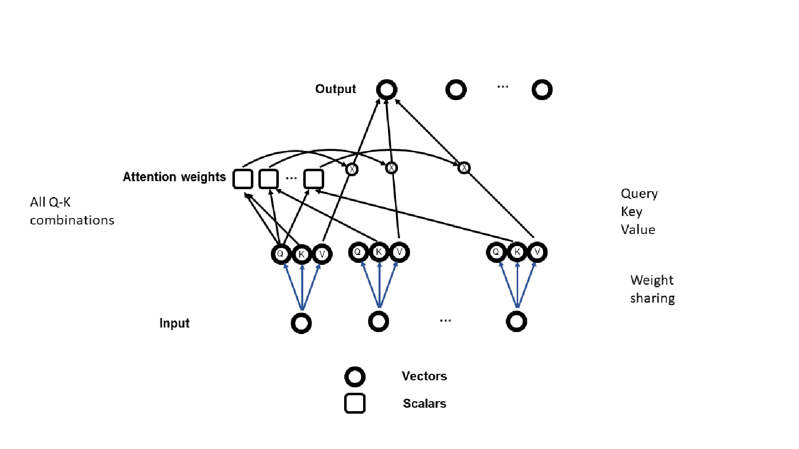
Although the descriptions of attention mechanisms in deep learning often seem complex and sometimes obscure the underlying neural architecture [16, 12, 21, 4, 13, 24], it can be checked that in all cases these are built out of the output and synaptic gating operations described in the previous section. For conciseness, here we demonstrate this in detail only for the transformer architectures [28, 27] (see also [20] for an MLP alternative to transformers). These architectures consist of stacks of similar encoder and decoder modules, with attention mechanisms in each module. The details of an encoder module are shown in Figure 5. As the Figure shows, a shared and typically linear network is first applied to each of input vectors. At the bottom of the architecture, these input vectors could represent for instance vectors encoding successive words from a sentence. At higher levels of the stack, these vectors could be associated with the outputs of the previous encoder or decoder module and correspond to more abstract representations. For each input vector, the shared network typically produces a triplet of vectors of the same size : (Query), (key), and (value), for a total of triplets. The subsequent attention mechanism is drawn in a concise way in the Figure and is based on three operations: (1) taking all pairwise dot products of the query vectors with the key vectors; (2) applying a softmax to each row of dot products; and (3) using the output of the softmax operations as weights for linearly combining the value vectors to produce the corresponding output vector at each position. The first operation can be built using output gating, each dot product involving gating operations, to multiply the proper and components together. As a side note, these dot products can be viewed as similarity measures between the and vectors, especially when these are normalized, and this suggests other kinds of transformer architectures where different similarity kernels are used. The softmax operation is a standard extension of the SM (Figure 10). The third operation corresponds to synaptic gating of the connections between the vectors and the outputs. The convex combination of the value vectors by the corresponding softmax weights determines how much each value vector influences each output vector, based on the corresponding similarities between vectors and vectors. This is where the influence of some of the value vectors can be enhanced, while the influence of others can be suppressed. Thus in total there are output gating operations, and synaptic gating operations (assuming output vectors). Thus, in short, the entire encoder module is based on a large number () of gating operations, both of the output and synaptic type. Thus, in this form, it can only be applied when is not very large. The basic transformer decoder module (not shown) is very similar. One important property of the encoder module conferred by the attention mechanisms is that the output is invariant under permutation of the inputs. This is because any permutation of the inputs, results in a corresponding permutation of the Q,K, and V vectors due to the weight sharing. This in turn induces a corresponding permutations in the dot products and softmax outputs, so that in the end the weighted contribution of any V vector into any output vector remains the same. This may seem surprising for an architecture that was originally developed for NLP tasks, where the order of the words obviously matter. Indeed, very often in practice positional information is added to each input vector. The permutation invariance of transformers is particularly beneficial for applications of transformers outside of NLP, in particular applications where the input consists of sets of data vectors, where the order of the data vectors does not matter (e.g. [19, 15]).
4. Functional Aspects of Attention
Next we study though several examples how certain functionalities can be implemented using attention mechanisms, beginning with the effect of attention on single units.
4.1. Single Unit Output Gating: Shaping the Activation Function
First, for simplicity, we consider output gating of a unit by another unit with the same inputs and the same weights, hence the same activation . The two units may have two different activation functions and . Through output gating, the final output of the gated unit will be given by: . Thus, in this case, output gating is equivalent to changing the activation function of the gated unit from to . Examples of this effect are shown in Figure (Figure 6) where both and are piecewise linear, and centered at the origin. Note that in the case of a linear unit gated by another linear unit, the final output is a quadratic function of the inputs, but with only parameters as opposed to . The ReLU activation function emerges naturally, through the gating of a linear function by a threshold function, or vice versa. Finally, the symmetric wedge activation function [26] emerges also naturally through the gating of a linear function by a threshold function.

4.2. Single Unit Attention: XOR
Next, we look at the simple XOR function. It is easy to show that the XOR function cannot be computed in a shallow way by a single linear threshold gate (or sigmoidal) neuron. Its computation requires at least one hidden layer. However, as shown in Figure 7 using 0/1 outputs, the XOR function can be computed by a shallow network with a single linear threshold unit output-gated by another linear threshold unit. To see this, note that any corner of the hypercube can always be isolated by a hyperplane from the other corners of the hypercube, i.e. there is always a linear threshold gate that has value 1 (resp. 0) for one Boolean setting of its inputs, and 0 (resp. 1) for all the other possible inputs (see Lemma 5.1). In particular, both the OR and NAND functions are of this kind and thus can be implemented by a linear threshold gate. Gating the OR by the NAND (or vice versa) produces the desired XOR function without using any hidden layers, assuming that the ouput gating operation is an integral part of the layer where it occurs.

4.3. Attention Layers: Universal Approximation Properties
Next, we look at how universal approximation proofs are affected if output gating is allowed, both in the Boolean and continuous cases.
4.3.1. The Boolean Case.
Every Boolean function of variables can be computed by a feedforward network of linear threshold gates, since AND, OR, and NOT can be implemented by linear threshold gates. By expressing the function in disjunctive or conjunctive normal form, the implementation can be achieved with a single hidden layer of exponential size. If we allow output gating, and its iterations, we have the following theorem.
Proposition 4.1.
Every Boolean function of variables can be expressed as the product of at most linear threshold gates, both in the and representations.
Proof.
Let be a Boolean function of variables, using to denote false and true respectively. If is 0 everywhere, it can immediately be expressed as a linear threshold gate. Likewise, if is 0 everywhere but one point of the dimensional cube, then it can be immediately expressed as a single linear threshold gate. Thus we can assume that is 0 on at most points. Let () denote the inputs where is zero. For each index , let denote the linear threshold gate which has value on and everywhere else. Then it is easy to check that can be written as the product (alternatively, on can express in conjunctive normal form). The proof is the same in the case, letting be the linear threshold gate with value for , and everywhere else. Obviously the same result holds for polynomial threshold gates of degree . ∎
In the case, the set of all Boolean functions with the multiplication operation forms a commutative group, and each Boolean function is its own inverse. The subset of all linear threshold gates contains the identity, and each linear threshold function gate is its own inverse. However it does not form a subgroup because it is not closed. By the theorem above, the multiplicative closure of the set of all linear threshold gates is the set of all Boolean functions.
Since every Boolean functions can be written as a product of an exponential number of linear (or polynomial) threshold gates, it is natural to ask whether a smaller number of factors may be used. Can every Boolean function be written as the product of a linear or polynomial number of linear threshold gates? We will answer this question negatively in Section 6.1.1.
4.3.2. The Continuous Case.
Next we look at the continuous case, using output gating to modify the basic universal approximation proof [6].
Theorem 4.2.
Let be a continuous function from to , and . Then there exists an integer such that can be approximated within everywhere over by a network of linear units, attended by corresponding linear threshold gates with output gating. The final approximation corresponds to the dot product between the vector of linear unit outputs and the vector of attending unit outputs.
Proof.
Since is continuous over the closed interval, it is uniformly continuous so that there exists such that for any and in :
| (4.1) |
Let us choose an integer large enough so that . Next we slice the interval into slices of width . Next we construct a network with linear units and linear threshold gate attention units with outputs in (the proof can be adjusted to accommodate outputs in ). All the attention units are connected to the single input by a weight equal to 1. Their threshold (bias) however are so that when only the first attention unit is on, when only the first two attention units are on, and so forth. In other words, the slice containing is encoded in the number of linear threshold gates that are on. For the linear units, they compute values as follows. The first linear unit approximates the function in the first slice by producing the line that goes through and , i.e. by implementing the function . The second linear unit approximates the function in the second slice by producing the line that goes through and , but with the subtraction of the value produced by the previous unit. Thus in short: . More generally, the output of the -th linear unit approximates the function in the -th slice producing the line that goes through and , but with the subtraction of . [Note: as an alternative construction, the linear units could also be taken to be constant, with , and .]
∎
The same construction can be applied over any closed interval, as well over any finite union of closed intervals. Furthermore, if the range is , the same construction can be applied to each component. And finally, the same construction can be generalized if the input domain is of the form . Thus in short:
Theorem 4.3.
Every continuous function from a compact set to can be approximated to any degree of precision by a shallow attention network comprising linear units gated by corresponding linear threshold gate units, with a final dot product output.
4.4. Attention Layers: Dot Products
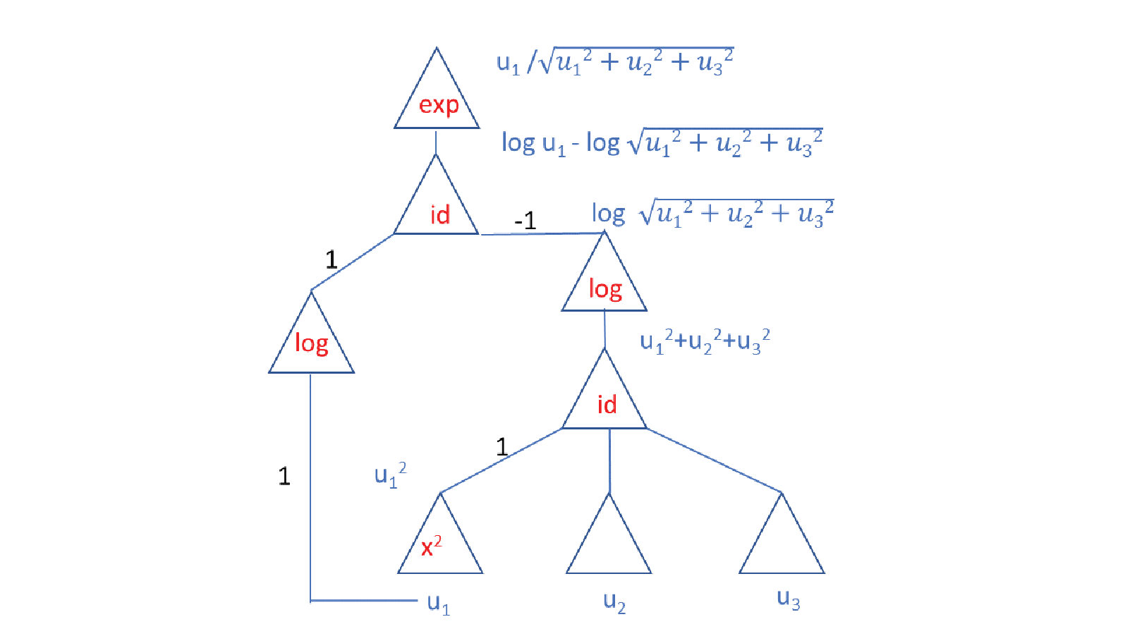
As we have seen in the section on transformers and the universal approximation proof above, one place where attention mechanisms are particularly important is for computing the dot product between two activity vectors and , associated with two corresponding layers of neurons each. This can be achieved through output gating to first compute all the pairwise products and then combine these products through a single linear output unit, with all its incoming weights set to , to compute the dot product . However, this dot product can equally be computed by synaptic gating, i.e. by using the vector to gate the incoming weights of the linear unit above and compute the dot product in the form . This can be scaled up to tensors where there are multiple output vectors and multiple attention vectors of the same length, and all pairwise dot products are computed, for any pair, as in the transformer architectures. Of course the dot product can also be computed in the standard model (Figure 8) however this requires a deeper network with four layers of standard units with fixed connections all equal to , and both logarithm and exponential transfer functions. Thus output or weight attention create a new primitive, or compact circuit, for computing dot products. The same is true of other operators that are often introduced in neural network without being part of the standard model, such as for the already-mentioned softmax (Figure 10) or the normalization of a vector (Figure 9).

4.5. Attention Layers: Attention Weights
Synaptic gating of a connection can suppress or enhance the corresponding incoming signal. Synaptic gating all the incoming edges of a unit allows to assign different importance to its different inputs. In addition, it is often desirable that these degree of importance form a probability vector, as in the transformer architecture, and this can be achieved through a softmax operation. It is possible to apply a normalizing softmax either to the vector of pairwise products , or to the rows or columns of the tensor of dot products , as in the transformer architectures. The output of these softmax operations can then be used to gate other synaptic weights. These gated weights are often equal and set to one in order to compute convex combinations, as in the transformer architecture Thus, in short, in transformer and other architectures, attention mechanisms allow dot products, softmax, and synaptic gating operations to be combined into one macro operation, which would require a network of depth for its implementation inside the SM.

5. Cardinal Capacity Review
We have seen that attention mechanisms enable important functionalities with minimal depth compared to the equivalent SM circuits, at the cost of adding attention neurons and mechanisms. Here we want to better understand the trade offs between the computations that are enabled and the corresponding costs. The key concept for doing so is the concept of cardinal capacity [10] which we briefly review below.
5.1. Definition of Capacity:
Given a class of functions , we define its cardinal capacity , or just capacity, to be: , where is the cardinality of in the finite case. In the continuous case, can be defined as a volume, but here we will focus primarily on finite cases. The class of all Boolean functions of variables has capacity . Here we will consider subclasses of , in particular those implemented by feed-forward networks of linear or polynomial threshold gates, with attention mechanisms, and compute the corresponding capacity.
5.2. Linear and Polynomial Threshold Functions
Linear or polynomial threshold functions are reasonably good approximation of linear- or polynomial-activation neurons with steep sigmoidal activation functions and, as such, are not particularly restrictive. A polynomial threshold functions of degree has the form , where is a polynomial of degree using a output representation. Alternatively, for a 0/1 output representation, we can use the form where is the Heaviside function equal to 0 for and to 1 otherwise. Units with values in are similar to logistic sigmoidal units, and units with values in are similar to sigmoidal units.
We let denote the class of polynomial threshold functions of degree . Thus denotes the class of linear threshold functions. When the inputs to a threshold function are binary, we use the term threshold gate. In the case of polynomial threshold gates, it does not matter whether their input is encoded using or (or for that many any two distinct real numbers). This is because there is an affine transformation between any two such encodings and the affine transformation can be absorbed in the synaptic weights, i.e. the coefficients of . The same is generally true for the encoding of the output, however when attention gating is considered the and encodings behave differently. For instance, in the case of output gating, the product of two threshold gates behaves like an AND, whereas the output of two gates behaves like an NXOR.
Thus to derive more general results, we will consider the case where the gating mechanism is implemented by a Boolean function , which could be an AND, an NXOR, or something else. In the most general setting, we let be a Boolean formula in variables. We are interested in the class of functions of the form where . We denote this class by .
5.3. Why Capacity is Important
The capacity is a measure of what the class of functions can do. As a single number, it is of course a very crude representation of the true functional capacity. However in the case of neural networks the capacity has a stronger significance. To see this, note first that the cardinal capacity is also the number of bits required to specify an element of . Thus in the case of neural networks, to a first order of approximation, the capacity is the number of bits that must be transferred from the training data to the synaptic weights during learning for the network to learn to implement a specific function in the class .
5.4. Capacity of Single Units: Review
Before we estimate the capacity of single units with attention mechanisms, we must review the known capacity results on single units without attention mechanisms. For a single linear threshold gate of variables, we have [31, 32]:
| (5.1) |
This result was refined to the form [18]:
| (5.2) |
Similar results have been obtained for polynomial threshold gates of degree [5, 11]. In particular, for any and satisfying (where is fixed and ) there exists a constant such that:
| (5.3) |
where:
| (5.4) |
For degree , including fixed degree , Equation 5.3 yields:
| (5.5) |
5.5. Activation Attention and Muliplexing
We now describe one of the main techniques that will be used in the attention capacity proofs for both synaptic and output gating. Perhaps surprisingly, this technique can be viewed as a form of attention, specifically a form of activation attention or multiplexing. It was developed and used in [9, 10]. First, we need the following lemma, stated for the 0/1 -dimensional hypercube, but equally valid on the -/+ hypercube, or any other hypercube . The lemma basically states that any vertex of the hypercube can be separated from the rest of the cube by a hyperplane with large margins.
Lemma 5.1.
Let be the -dimensional hypercube, and and . Fix any vertex of the hypercube, and let . Then there exists affine linear functions of the form such that: and for any .
Proof.
First note that there are 1:1 affine maps between the different hypercubes, thus it is enough to prove the result for the 0/1 hypercube. Second, all the corners play a symmetric role so it is enough to prove it for the corner . It is easy to check that: satisfies the conditions of the Lemma. Note that by using the sign of the regions and corresponding margins can be exchanged ( and for all ). ∎

Now consider a neural network consisting of inputs fully connected to a hidden layer of linear or polynomial threshold functions (Figure 12) . In the multiplexing approach, we add , or even just new binary inputs to the input layer. different binary patterns over these inputs can be associated in one to one fashion with one of the threshold functions in the hidden layer. Let be any integer and let denote the corresponding pattern of bits. For simplicity we can just use the binary representation of , but any other representation works equally well.
This pattern can be viewed as a corner of the corresponding hypercube of dimension and thus we can apply Lemma 5.1 above to choose the weights connecting the attention units and the bias to hidden unit accordingly. In particular, the weights can be chosen such that: (1) the attending signal originated from the attending bit patterns is equal to 0; and (2) for all other settings of the attending bits, the attending signal is arbitrarily large and negative (alternatively arbitrarily large and positive). Ans similarly for all the other units and attention input patterns. As a result, whenever appears in the attention bits, the -th output of the hidden layer is equal to , and for all the other settings of the attention bits, the output is constantly equal to 1, or constantly equal to 0 (or -1 in the case of threshold hidden units). The pattern of constant bits is called the mask and different masks can be used for different proofs. Thus, in short, the attending signal emanating from the attention units is multiplexed with the regular signal and used to focus the attention of the hidden layer on the hidden unit encoded by the bits appearing in the attention units. The output of the hidden layer is equal to the mask except for the attended position, where it is equal to the corresponding function .
This form of activation attention is the key tool for proving capacity lower bounds. To see this, consider for instance the case where an OR operator is applied to the outputs of the hidden layer. With a mask consisting of 0s, when the attention bits are set to , the output of the OR applied to the hidden units is equal to . Thus the truth table of the overall input-output function of the original inputs plus the attention bits is uniquely equal to when the attention bits are set to . Thus the capacity of the network with the expanded input of size is lower bounded by the sum of the capacities associated with the functions over the original input of size .

6. Capacity of Single Unit Attention
We can now begin to estimate the capacity of various attention circuits, when the attention signal originate in a single gating unit, as shown in Figure 13.

6.1. Capacity of Single Attention Units: Output Gating
We want to compute the capacity of the class of all functions that can be computed by one neuron gated by another neuron, corresponding to the left hand side of Figure 13. In the purely linear case,we have seen that this is the set of all quadratic functions of the form . To partially address this question in the non-linear case, we can consider first the case of a linear threshold gate gated by another linear threshold gate, and then similarly for polynomial threshold gates of degree . Using linear threshold gates for the gated and the gating units, this is the class of Boolean functions of the form:
| (6.1) |
This class contains the identity and all the linear threshold gates. Thus, by Zuev’s result (Equation 5.1) its capacity is at least . However, intuitively, it must contain many other functions as shown in Figure 14 suggesting that in general the product of two linearly separable functions is not linearly separable. On the other hand, the upperbound on the capacity is at most , because the capacity is always bounded by the sum of the capacity of each individual component. Similarly considerations can be made for the which leads to the more general problem of estimating the capacity of the class of functions of the from where is any Boolean operator, and and are linear or polynomial threshold gates. And even more generality can be obtained by considering classes of Boolean functions of the form where is a -ary Boolean operator and are polynomial threshold gates of respective degrees . We first address the case of and then the general case.

6.1.1. Pairwise Composition ().
| Irred. () | Sym | LTG | C{B(f,g)}) | ||
| no | yes | yes | |||
| no | no | yes | |||
| no | no | yes | |||
| yes | yes | yes | |||
| yes | no | yes | |||
| yes | no | yes | |||
| yes | yes | yes | |||
| yes | yes | no |
For completeness, consider Table 2 summarizing all 16 Boolean function of two variables. We can substitute and with arbitrary linear (or polynomial) threshold functions and and compute the corresponding cardinal capacity. The first group in the table correspond to always true (T) and always false (F) functions, thus to a negligible total capacity of 1. The second group corresponds to a single linear threshold function, and thus its capacity is equal to: All the elements in the second group in the table are also found in the third group corresponding to the AND and OR operators, because . Within the third group, all the OR expression are equivalent to each other, and all the AND expressions are equivalent to each other, when and are substituted with linear (or polynomial) threshold gates. This is because whenever is a polynomial threshold gate of degree , then is also a polynomial threshold gate of degree . The first three groups cover 14 Boolean functions in total. These 14 Boolean functions can be implemented by a single linear threshold gate of and , and no other linear threshold gate of and exist. Thus the total aggregated capacity corresponding to all these cases, is given by the cardinal capacity of a network of linear threshold gates with inputs, 2 hidden units, and 1 output unit. This capacity is given by [8, 10]:
| (6.2) |
There is a one-to-one correspondence between the set and the set through the negation operator. Therefore:
| (6.3) |
[Note that any Boolean function that isolates once corner of the hypercube is irreducible. For such a function, knowing the values of the sequence uniquely determines the values of and ]. The relevant result in [8, 10] is obtained using the attention multiplexing technique, applied in fact with the OR Boolean function and a mask of 0s, as described in Section 5.5. Thus, in short:
| (6.4) |
For the last row of the table, the output gating (multiplication) of two linear threshold functions correspond to applying the negation of the XOR Boolean operator. Note that: and . As a result we have:
| (6.5) |
when and vary over all possible linear threshold gates. Even more strongly, the corresponding sets of Boolean functions are identical:
| (6.6) |
Now it is easy to see that
| (6.7) |
The lower bound is obtained by noticing that for any Boolean function , . The upperbound is obtained by noticing that can be implemented by a network of linear threshold gates (using the disjunctive normal form), and the capacity of such a network is always at most equal to the sum of the capacities of its individual gates. Finally, the attention multiplexing technique described in Section 5.5 applied with a mask of 1s (since ) shows that:
| (6.8) |
Thus the product of or linear threshold gates have the same capacity, and a similar argument holds for polynomial threshold gates. These results can be summarized in the following theorem, which is true for both and threshold gates:
Theorem 6.1.
The capacity of a linear threshold gate output-gated by another linear threshold gate is given by:
| (6.9) |
Likewise, the capacity of a polynomial threshold gate of degree output-gated by another polynomial threshold gate of the same degree is given by:
| (6.10) |
Remark 6.2.
Furthermore, we have seen that every Boolean function can be written as a product of linear threshold gates with an exponential number of terms (Proposition 4.1). Theorem 6.1 shows that it is not possible to do so using only a polynomial number of terms, since this would result in an overall capacity that is only polynomial, whereas the capacity of is .
Remark 6.4.
These results can be extended to other interesting cases. For instance, if we assume that the weights of the gated and gating linear threshold neurons are binary with values, then the output gating capacity is equal to .

6.1.2. General Composition ().
The results in the previous section can be generalized to the class of functions of the form , where is a Boolean function of variables and, for each , . We denote this class by: .
Theorem 6.5 (Composition).
Let be an irreducible Boolean operator in variables.22 2 Irreducibility means that can not be expressed as a Boolean operator in fewer than variables. Then:
| (6.11) |
Furthermore, if is the set of all irreducible Boolean functions of two variables (there are 10 of them), we have:
| (6.12) |
where the intersection is over the ten irreducible binary Boolean operators.
6.2. Capacity of Single Attention Units: Synaptic Gating
We are now ready to compute the capacity for the case corresponding to the right hand side of Figure 13, where one threhsold unit synaptically gates the weights of another threshold unit. To begin with, we look at the case where all the weights of the gated unit are gated simultaneously. The main result is as follows:
Theorem 6.6.
Let and be two linear or polynomial threshold gates (not necessarily of the same degree), both with the same or output encoding and binary input variables. Then full synaptic gating of by , where all the coefficients of are multiplied by , is equivalent to output gating of by . In particular, if both gates are linear threshold gates, then the corresponding capacity is given by:
| (6.16) |
and if both gates are polynomial threshold gates of degree , then the corresponding capacity is given by:
| (6.17) |
Proof.
We sketch the proof when and are linear threshold gates, but the argument extends immediately to polynomial threshold gates. Let us assume that and . Then, with full synaptic gating, the gated function satisfies: . In the case of units, if is the Heaviside function, then: . If , this is the same as . Likewise if , as long as we define , then is also equal to: . [Note that the gating is applied to the bias too]. ∎
Remark 6.7.
In this particular case, to some extent, we can also consider the mixed case. If is a gate and is a gate, if we define then we also have everywhere. If is a gate and is a gate, then when we also have . However, when , then .

Remark 6.8.
Finally, we consider the synaptic gating case where the gating unit gates only one of the weights of the gated unit (Figure 16). The following Proposition provides bounds on the corresponding capacity.
Proposition 6.9.
Consider the case of a linear threshold gate with binary inputs, where one of the weights is synaptically gated by the output of a second linear threshold gate of the same inputs. Then the capacity satisfies:
| (6.18) |
If the linear threshold gates are replaced by polynomial threshold gates of degree , the capacity satisfies:
| (6.19) |
The same bounds hold for the case of additive activation attention between two linear polynomial threshold gates, or two linear polynomial threshold gates, of the same inputs.
Proof.
The result is true for both and encodings of the outputs. We provide the proof in the linear case but the technique is the same for polynomial threshold gates of degree . The lower bound results immediately from the fact that the gating unit could have an output constant and equal to 1 ). In this case the gated function is equal to and the lower bound is the corresponding capacity estimate. The upperbound is simply the sum of the capacities. A similar argument applies for the case of additive activation attention. ∎
7. Capacity of Attention Layers
The previous attention results are obtained using only two neurons, a gating neuron and a gated neuron, with either output gating or synaptic gating. We now extend the capacity analysis to cases where there is a layer of gating neurons, as shown in Figure 17 for both output and synaptic gating.

7.1. Capacity of Attention Layers: Output Gating
We now examine the capacity of a network with one attention layer with output gating, as depicted on the left hand side of Figure 17. Thus we consider an architecture with inputs, hidden linear threshold units gated by corresponding linear threshold units, and one final linear threshold output gate. All the linear threshold gates have outputs, although the following theorem is unchanged, and the method of proof is similar, if the gates have 0/1 outputs. We denote by the corresponding set of Boolean functions. Note that this is the same architecture for computing the dot product of the gated and the gating hidden layer outputs, except that the final unit is non-linear with variable weights, instead of being linear with fixed weights equal to one. We will also let denote the set of Boolean functions corresponding to one linear threshold gate of variables output-gated by another linear threshold gate of the same variables.
Theorem 7.1.
The capacity of the set of Boolean functions corresponding to inputs, hidden linear threshold gates output-gated by hidden linear threshold gates of the same inputs, followed by one linear threshold gate output satisfies:
| (7.1) |
for , and for any choice of . Furthermore:
| (7.2) |
Thus:
| (7.3) |
Proof.
Let us denote by the map between the input layer and the hidden layer with gating, and by the map from the hidden layer to the output layer. For the upper bound, we first note that the total number of possible maps is bounded by , since consists of threshold gates gated by threshold gates, and thus each gated unit corresponds to at most possibilities by the Theorems in Section 6. Any fixed map , produces at most distinct vectors in the hidden layer. It is known [1] that the number of threshold functions of variables defined on at most points is bounded by:
| (7.4) |
using the assumption . Thus, under our assumptions, the total number of functions of the form is bounded by the product of the bounds above which yields immediately:
| (7.5) |
For the lower bound, we can force the gating units to be the identity (i.e. with a constant output equal to 1). In this particular case, the gating units can be ignored and we need to count the number of Boolean functions that can be implemented in the remaining architecture. A theorem in [10] shows that this number is equal to .
To prove the rest of the theorem, we use attention multiplexing. As a reminder, the basic idea is to have a small set of the input units act as attention units that can be used to select a particular function in the hidden layer. The same setting of the attention units will be used to select the corresponding functions in both the gating and gated layers. More formally, we decompose as: where corresponds to the attention units. Likewise, we decompose each input vector as: , where:
| (7.6) |
For any gated Boolean linear threshold map from to , we can uniquely derive a map from to defined by:
| (7.7) |
Here signifies that the binary vector represents the digit . In other words is used to select the -th unit in the gated layer as well as in the gating layer, and filter by retaining only the value of . By Lemma 5.1), this selection procedure can be expressed using a single linear threshold function of the input for the gated layer, and similarly for the gating layer. We say that is obtained from by multiplexing and is a gated threshold map. It is easy to see that the filtering of two distinct maps and results into two distinct maps and . Now let us use in the top layer–note that OR can be expressed as a linear threshold function. Then it is also easy to see that . Thus the total number of Boolean functions that can be implemented in this architecture is lower-bounded by the number of all gated Boolean maps . This yields:
| (7.8) |
using the fact that , and by assumption. Thus: . ∎
Remark 7.2.
In Theorem 7.1, we see again that both the capacity and the number of parameters approximately double at the same time.
7.2. Capacity of Attention Layers: Synaptic Gating
We now examine the capacity of a network with one attention layer with synaptic gating, as depicted on the right hand side of Figure 17, with each gating neuron gating a different weight of a gated neuron.
Proposition 7.3.
Consider the case of a linear threshold gate with inputs and weights, where each weight is synaptically gated by an independent linear threshold gate of the same inputs. Then the capacity satisfies:
| (7.9) |
If the linear threshold gates are replaced by polynomial threshold gates of degree , the capacity satisfies:
| (7.10) |
Proof.
The proof is similar to the proof of Proposition 6.9. The lower bound is obtained by constraining all the gating units to have a constant output equal to 1. The upperbound is simply the sum of all the capacities. ∎
Likewise, we can consider an architecture with inputs, one layer of gating units, and one parallel layer of gated units. Each gating unit is uniquely paired with one gated unit (one to one) and synaptically gates one of the weights of the gated unit.
Proposition 7.4.
Consider the case of an architecture with inputs, one layer of gating units, and one parallel layer of gated units. Each gating unit is uniquely paired with one gated unit (one to one) and synaptically gates one of the weights of the gated unit. Then the capacity satisfies:
| (7.11) |
If the linear threshold gates are replaced by polynomial threshold gates of degree , the capacity satisfies:
| (7.12) |
Proof.
The proof is similar to the proof of Proposition 6.9. The lower bound is obtained by constraining all the gating units to have a constant output equal to 1. The upperbound is simply the sum of all the capacities. ∎
8. Conclusion
In addition to the fundamental role attention plays in brain function, attention mechanisms have also become important for artificial neural networks and deep learning. Here we have taken the first steps towards building a theory of attention mechanisms by first identifying the quarks of attention, i.e. its smallest building blocks. Using the three variable types of the SM allows for the systematic identification and organization of possible attention building blocks based on their origin type, target type, and whether the mechanism of action is additive or multiplicative. Assuming that the attention signal originates from the output of some neurons, this yields six possibilities, which can then be reduced to three main cases: activation attention, output gating, and synaptic gating. Activation attention falls within the SM, whereas output gating and synaptic gating correspond to multiplicative extensions of the SM. Current attention-based architectures in deep learning, including transformers, are built out of attention modules which are themselves built out of output gating and synaptic gating operations. These operations and modules can be viewed as new primitives in the language of neural architectures in digital simulations and, because they are differentiable, the usual backpropagation learning framework can easily be extended to them. However, in a physical neural machine, these operations require additional connections (wires) and physical mechanisms for implementing multiplicative interactions.
Ouput gating can be used dynamically to directly silence unattended neurons, and to magnify the output of attended neurons. It can also be used as the main building block of a shallow module that can compute the dot product of two vectors of neuronal activities. The latter is a key, massively used, component of transformer architectures.
Synaptic gating is a fast synaptic mechanism that can be used dynamically to silence or weigh the attended synapses. It is often used in combination with a softmax operator to enable dynamic convex combinations of vectors, as in the transformer architectures. The concept of fast synapses that can vary their strengths on fast time scales is not new and has been associated with different roles, in different contexts. For instance, one potential role is the storage of transient information, such as intermediary results during mental reasoning, or simply the memorization of the beginning of a paragraph as the reading of the paragraph proceeds. A second potential role stems from viewing synaptic weights as computer programs, and thus fast synapses as enabling dynamic changes in the programs that are being executed and the implementation of parameterized functions. And a third role studied here is the enabling of attention. These three roles are not independent and raise interesting architectural questions for deep learning and neuroscience and the possible need for multiple synaptic time scales interacting in hierarchical ways.
To see this, as an example, consider the reading paradigm where information about the first sentence of a long paragraph is stored using a set of fast weights. If, as the reading proceeds, one must suddenly access a specific subset of this transiently stored information, attention must be directed towards certain particular words contained in the first sentence. In a deep learning architectures, this can be thought of in terms of a softmax synaptic gating, as is done in transformer and other NLP architectures. Thus somehow this fast weight attention mechanism must operate upon, and be faster than, the fast weight synaptic mechanism used to store information about the first sentence.
Attention mechanisms allow the attending network to modulate the function computed by the attended network, thereby expanding the scope of useful functions that can be efficiently implemented and trained in deep learning. Because the SM already has universal approximation properties, its extensions should not be evaluated in terms of which functions can be approximated, but rather in terms of other efficiencies. While attention blocks act as new primitives in standard deep learning software libraries, having access to output gating and synaptic gating mechanisms in a physical neural network can reduce its depth. Using the notion of cardinal capacity, and working with the approximation provided by Boolean neurons (linear or polynomial threshold gates), enables systematic investigations of the capacity of attentional circuits that were previously not possible. In particular, we have been able to estimate the capacity of basic attentional circuits involving linear, or polynomial, threshold gates. In many cases of interest, we found essentially a doubling of the capacity with a doubling of the number of parameters, which is a sign of efficiency.
Perhaps surprisingly, a key ingredient in the capacity proofs is the third form of attention, activation attention. Activation attention is used to prove capacity lower bounds by the multiplexing approach which selects a unit in a layer, as a function of the attending units, while driving the remaining units in the layer to low or high saturation. There is work left for tightening some of the estimates and for extending them to other activation functions and other architectures.

Overall, both output and synaptic gating are extensions of the SM which introduce quadratic terms in the SM (Figure 18). Quadratic terms are powerful but expensive: a neuron with full quadratic activation over its inputs requires on the order of synaptic parameters. Using quadratic activations everywhere in a large deep architecture leads to implementations that may not be efficient in terms of parameters and learning. Attention mechanisms are a way of introducing quadratic terms in a sparse way, in order to gain some of the benefits of quadratic activations, without paying the full price.
Finally, we can return to the quotes in the introduction linking attention to awareness and pointing to the inadequacy of having a single term. While subjectively we feel that we can control and direct our attention and be aware of its shifts, it should be obvious that attention mechanisms, such as output or synaptic gating, are computational mechanisms that do not require awareness. They can operate at all levels of a cognitive architecture, for instance to help implement dynamically whole-part hierarchies and ultimately awareness itself. Thus, in short, awareness is not necessary for attention, but attention may be necessary for awareness. Having a single term is indeed inadequate and, in time, it may have to be replaced with multiple terms to better capture the underlying complexities.
9. Appendix: Detailed Proof of Theorem 6.5
Here a polynomial threshold function is a function of the form where is a polynomial in real variables of degree at most . The class of all such functions is denoted .
Let be a Boolean function in variables. We are interested in the class of functions of the form where . Denote this class by . We want to prove the following theorem:
Theorem (Composition). Let be an irreducible Boolean operator in variables. Then:
| (9.1) |
The upper bound is trivial from considering the total number of tuples with . The lower bound is nontrivial except for where both bounds become identical. The key to the proof is the multiplexing (activation attention) procedure, where input components are viewed as attention units capable of producing a constant mask in the hidden layer, except for the attended function. Here for simplicity we use a sparse encoding in the components, although dense encoding is also possible, as in the proof of Theorem 7.1. Dense encoding would lead to a reduction in the number of attending units from to as in Section 5.5. As a side note, using more attention units than the minimal number required, can be used to reduce the size of the attention weights, or to make the attention mechanism less sensitive to each individual attention bit.
To prove the lower bound in Composition Theorem 6.5, let us restate it equivalently as:
| (9.2) |
Irreducibility implies that if we select any input component , the value of cannot be determined entirely from the value of the remaining components alone. More formally:
Lemma 9.1.
Consider an irreducible Boolean operator and an index . There exist signs and , , such that:
| (9.3) |
Proof.
Consider as a function of . If this function is constant in the variable no matter how we fix the other variables, then the value of is entirely determined by the values of these other variables, which contradicts irreducibility. Therefore, there exists some assignment , , so that the function is not constant in . But there exists only two non-constant Boolean functions in one variable: or , and this determines . ∎
The next lemma essentially states that we can fit an affine function of variables to points.
Lemma 9.2.
Let and denote the canonical basis vectors in . Then, for any choice of index and signs , there exists an affine function such that:
| (9.4) |
for all .
Proof.
It is straightforward to check that the function:
| (9.5) |
satisfies the required property. ∎
We can now use the previous lemma to derive a lemma for consistently extending a function of variables to a function of variables. Here components are used as selector of filter variables, as in the proof of Theorem 7.1.
Lemma 9.3.
Consider a function , an index , and signs and , . There exists a function such that:
| (9.6) |
for all . Here denotes the concatenation operator.
Proof.
Express the polynomial threshold function as:
| (9.7) |
where is a polynomial in variables and of degree at most . Let be a function that satisfies the conclusion of Lemma 9.2. Fix a number large enough so that for all , and define:
| (9.8) |
for all and . By construction, is a polynomial threshold function on of degree at most as required.
Let us check that satisfies the conclusion of the lemma. If , we have due to our choice of (per the conclusion of Lemma 9.2), and we get . If with , then our choice of implies . The choice of guarantees that the term dominates the term in magnitude, so we have . ∎
We can now use Lemma 9.3 for the simultaneous extension and filtering of several functions of variables relative to an irreducible Boolean function .
Lemma 9.4.
For any -tuple of functions where there exists a -tuple of functions where such that:
| (9.9) |
for all and .
Proof.
Armed with this lemma, we can now prove Theorem 6.5.
Proof of Theorem 6.5.
Lemma 9.4 demonstrates that for any tuple of functions there exists a function such that for all and . Thus, each component of the original -tuple can be uniquely recovered from . Therefore, a map (if there are multiple corresponding to some , select one arbitrarily) defines an injection from the cartesian product into , completing the proof. ∎
As shown in Table 2, there are binary Boolean operators . Ten of them are irreducible, including AND, OR and XOR and their negations. For each such operator, the Composition Theorem 6.5 gives:
| (9.13) |
Surprisingly, the intersection of all ten classes is still as large.
Proposition 9.5.
We have:
| (9.14) |
where the intersection is over the ten irreducible binary Boolean operators.
In particular, there are many functions (specifically, that can be simultaneously expressed as: where all the are linear threshold gates.
Proof.
In the proof of the Composition Theorem 6.5 above, we showed that for each irreducible Boolean operator and pair of functions , there exists such that:
| (9.15) |
for all . Obviously, this pair of equations defines uniquely on , and is independent of . Thus, lies in the intersection of over all irreducible . ∎
Acknowledgment
Work in part supported by ARO grant 76649-CS and NSF grant 1633631 to PB, and AFOSR grant FA9550-18-1-0031 to RV.
References
- [1] Martin Anthony. Discrete mathematics of neural networks: selected topics, volume 8. Siam, 2001.
- [2] Amy F.T. Arnsten and Francisco X. Castellanos. Neurobiology of attention regulation and its disorders. Pediatric Psychopharmacology, page 95, 2010.
- [3] Jimmy Ba, Geoffrey E Hinton, Volodymyr Mnih, Joel Z Leibo, and Catalin Ionescu. Using fast weights to attend to the recent past. In Advances in Neural Information Processing Systems, pages 4331–4339, 2016.
- [4] Dzmitry Bahdanau, Kyung Hyun Cho, and Yoshua Bengio. Neural machine translation by jointly learning to align and translate. January 2015. 3rd International Conference on Learning Representations, ICLR 2015 ; Conference date: 07-05-2015 Through 09-05-2015.
- [5] P. Baldi. Neural networks, orientations of the hypercube and algebraic threshold functions. IEEE Transactions on Information Theory, 34(3):523–530, 1988.
- [6] P. Baldi. Deep Learning in Science. Cambridge University Press, Cambridge, UK, 2021.
- [7] Pierre Baldi, Kyle Cranmer, Taylor Faucett, Peter Sadowski, and Daniel Whiteson. Parameterized neural networks for high-energy physics. The European Physical Journal C, 76(5):235, 2016.
- [8] Pierre Baldi and Roman Vershynin. Neural networks capacity. arXiv preprint arXiv:xxxxx, 2018.
- [9] Pierre Baldi and Roman Vershynin. On neuronal capacity. In Advances in Neural Information Processing Systems, pages 7740–7749, 2018.
- [10] Pierre Baldi and Roman Vershynin. The capacity of feedforward neural networks. Neural Networks, 116:288–311, 2019. Also: arXiv preprint arXiv:1901.00434.
- [11] Pierre Baldi and Roman Vershynin. Polynomial threshold functions, hyperplane arrangements, and random tensors. SIAM Journal on Mathematics of Data Science, 1(4):699–729, 2019. Also: arXiv preprint arXiv:1803.10868.
- [12] Jan Chorowski, Dzmitry Bahdanau, Dmitriy Serdyuk, Kyunghyun Cho, and Yoshua Bengio. Attention-based models for speech recognition. arXiv preprint arXiv:1506.07503, 2015.
- [13] Jacob Devlin, Ming-Wei Chang, Kenton Lee, and Kristina Toutanova. BERT: Pre-training of deep bidirectional transformers for language understanding. In Proceedings of the 2019 Conference of the North American Chapter of the Association for Computational Linguistics: Human Language Technologies, Volume 1 (Long and Short Papers), pages 4171–4186, Minneapolis, Minnesota, June 2019. Association for Computational Linguistics.
- [14] Yihe Dong, Jean-Baptiste Cordonnier, and Andreas Loukas. Attention is not all you need: Pure attention loses rank doubly exponentially with depth. arXiv preprint arXiv:2103.03404, 2021.
- [15] M. Fenton, A. Shmakov, T. Ho, S. Hsu, D. Whiteson, and P. Baldi. Permutationless many-jet event reconstruction with symmetry preserving attention networks. Physical Review D, 2020. In press. Also arXiv:2010.09206.
- [16] Alex Graves, Greg Wayne, and Ivo Danihelka. Neural Turing machines. arXiv preprint arXiv:1410.5401, 2014.
- [17] Laurent Itti, Geraint Rees, and John K Tsotsos. Neurobiology of attention. Elsevier, 2005.
- [18] Jeff Kahn, János Komlós, and Endre Szemerédi. On the probability that a random1-matrix is singular. Journal of the American Mathematical Society, 8(1):223–240, 1995.
- [19] Juho Lee, Yoonho Lee, Jungtaek Kim, Adam Kosiorek, Seungjin Choi, and Yee Whye Teh. Set transformer: A framework for attention-based permutation-invariant neural networks. volume 97 of Proceedings of Machine Learning Research, pages 3744–3753, Long Beach, California, USA, 09–15 Jun 2019. PMLR.
- [20] Hanxiao Liu, Zihang Dai, David R So, and Quoc V Le. Pay attention to mlps. arXiv preprint arXiv:2105.08050, 2021.
- [21] Minh-Thang Luong, Hieu Pham, and Christopher D Manning. Effective approaches to attention-based neural machine translation. arXiv preprint arXiv:1508.04025, 2015.
- [22] Bruno A Olshausen and David J Field. Emergence of simple-cell receptive field properties by learning a sparse code for natural images. Nature, 381(6583):607, 1996.
- [23] Michael I Posner. Cognitive neuroscience of attention. Guilford Press, 2011.
- [24] Alec Radford, Jeff Wu, Rewon Child, David Luan, Dario Amodei, and Ilya Sutskever. Language models are unsupervised multitask learners. 2019.
- [25] Jürgen Schmidhuber. Learning to control fast-weight memories: An alternative to dynamic recurrent networks. Neural Computation, 4(1):131–139, 1992.
- [26] Mohammadamin Tavakoli, Forest Agostinelli, and Pierre Baldi. Splash: Learnable activation functions for improving accuracy and adversarial robustness. Neural Networks, 140:1–12, 2021.
- [27] Ashish Vaswani, Noam Shazeer, Niki Parmar, Jakob Uszkoreit, Llion Jones, Aidan N Gomez, Ł ukasz Kaiser, and Illia Polosukhin. Attention is all you need. In I. Guyon, U. V. Luxburg, S. Bengio, H. Wallach, R. Fergus, S. Vishwanathan, and R. Garnett, editors, Advances in Neural Information Processing Systems 30, pages 5998–6008. Curran Associates, Inc., 2017.
- [28] Ashish Vaswani, Noam Shazeer, Niki Parmar, Jakob Uszkoreit, Llion Jones, Aidan N Gomez, Łukasz Kaiser, and Illia Polosukhin. Attention is all you need. In Advances in neural information processing systems, pages 5998–6008, 2017.
- [29] Daniel LK Yamins and James J DiCarlo. Using goal-driven deep learning models to understand sensory cortex. Nature neuroscience, 19(3):356–365, 2016.
- [30] David Zipser and Richard A Andersen. A back-propagation programmed network that simulates response properties of a subset of posterior parietal neurons. Nature, 331(6158):679–684, 1988.
- [31] Yu A Zuev. Asymptotics of the logarithm of the number of threshold functions of the algebra of logic. Soviet Mathematics Doklady, 39(3):512–513, 1989.
- [32] Yu A Zuev. Combinatorial-probability and geometric methods in threshold logic. Diskretnaya Matematika, 3(2):47–57, 1991.