Plasmoid-fed prominence formation (PF²) during flux rope eruption

To investigate the FR eruption and the accompanied prominence formation, we solve the following set of resistive MHD equations:

where $\mathcal{H}=[\rho\varepsilon+(1/2)\rho\mathbf{u}^{2}+\mathbf{B}^{2}/8\pi]$ is the total energy density, $\varepsilon=p/(\gamma\rho-\rho)$ is the internal energy per unit mass, $\gamma=5/3$ is the adiabatic index, $\mathbf{E}=[\eta\mathbf{J}-(\mathbf{u}\times\mathbf{B})/c]$ is the electric field, $\eta$ is the resistivity, $\mathbf{J}=(c/4\pi)\nabla\times\mathbf{B}$ is the electric current density, $Q$ is the radiative loss rate, $h$ is the background heating rate, $\mathbf{g}$ is the gravitational acceleration, and $c$ is the light speed in vacuum. The set of MHD equations is closed by the equation of state

where $m_{\mathrm{H}}$ is the hydrogen atom mass and the mean molecular weight $\bar{\mu}=1.4/2.3$ for the fully ionized plasma with a $10:1$ abundance of hydrogen and helium. The gravitational acceleration $\mathbf{g}$, the radiative cooling term $Q$, and the thermal conduction are treated in the same way as Zhao et al. 2017; Zhao et al. 2019; Zhao & Keppens 2020. The heating function $h$ is chosen to initially compensate the radiative loss exactly, i.e., $h(x,y)=Q(\rho_{I},T_{I})$, where $\rho_{I}(x,y)$ and $T_{I}(x,y)$ are the initial density and temperature distributions.

The above equations are solved in two-and-a-half dimension, in a dimensionless form using the MPI-AMRVAC code (Nool & Keppens 2002; Porth et al. 2014; Xia et al. 2018; Keppens et al. 2021). To non-dimensionalize the equations, each variable is divided by its normalizing unit. The normalizing units are given in Table 1, and the units for derived variables are listed as well. The CGS-Gaussian units are used throughout the paper. The MHD equations are numerically solved with a finite-volume scheme setup combining the total variation diminishing Lax-Friedrich (TVDLF) scheme (Yee 1989; Tóth & Odstrčil 1996) with a third-order Cada limiter (Čada & Torrilhon 2009) for reconstruction, and a strong stability preserving Runge-Kutta four-step, 3rd-order time integration (SSPRK4), which is stable up to CFL of $\sim 2$ (Spiteri & Ruuth 2002).

Our simulation is conducted in a two-dimensional Cartesian simulation box covering the region $[-25L_{0},25L_{0}]\times[0,50L_{0}]$ in the x-y plane, where $L_{0}=10^{9}\,\mathrm{cm}$ is the typical length scale as listed in Table 1. The simulation box is divided into $256\times 256$ cells, which form the base computational grid. Up to $8$ adaptive mesh refinement (AMR) levels are used, and thus the finest grid size reaches $0.0015L_{0}=15\,\mathrm{km}$.

We adopt the same initial magnetic field configuration as in Takahashi et al. 2017, which is also provided in Appendix for convenience. We set the parameter $M_{q}$ as $0.8M_{c}$, with $M_{c}$ the critical value below which no FR equilibrium exists. The definitions of $M_{q}$ and $M_{c}$ are given in Takahashi et al. 2017 as well as in Appendix. The parameters $A_{0}$, $R_{0}$, $\delta$ and $H$ in Appendix are set as $A_{0}=20\,\mathrm{Gauss}$, $R_{0}=1.2L_{0}$, $\delta=0.1L_{0}$ and $H=R_{0}$, respectively, where $L_{0}=10^{9}\,\mathrm{cm}$ is listed in Table 1. The initial temperature distribution is chosen in line with Zhao et al. 2017; Zhao et al. 2019; Zhao & Keppens 2020. The height of the chromosphere-corona transition region is set as $0.2L_{0}=2\,\mathrm{Mm}$ initially. The chromosphere with a temperature of ${10}^{4}\,{\rm{K}}$ is located below the transition region, which is a thin layer compared to the large size of the simulation domain. The coronal temperature profile is chosen as a vertically stratified profile with a constant vertical thermal conduction flux (i.e., $\kappa\partial T/\partial y=2\times{10}^{5}\,\mathrm{erg}\,{\mathrm{cm}}^{-2}\,{{\rm{s}}}^{-1}$, where $\kappa={10}^{-6}{T}^{5/2}\,\mathrm{erg}\,{\mathrm{cm}}^{-1}\,{{\rm{s}}}^{-1}\,{{\rm{K}}}^{-3.5}$) above $0.2L_{0}=2\,\mathrm{Mm}$, following Xia et al. 2012. The initial density and pressure are then determined by assuming a hydrostatic atmosphere with a number density of ${10}^{14}\,{\mathrm{cm}}^{-3}$ at the bottom ghost cell boundary. An FR with the same density and temperature of the coronal plasma pre-exists in the low corona in this setup, while, in contrast, the initial configuration is a linear force-free arcade in Zhao et al. 2017; Zhao et al. 2019; Zhao & Keppens 2020. The resistivity is set as a uniform and constant parameter $\eta=2\times 10^{-5}\eta_{0}=3.2564\times 10^{-9}\,\mathrm{s}$ throughout the simulation domain, which gives a global Lundquist number $S_{Lu}\simeq 5\times 10^{5}$ in the global length scale $\sim 10L_{0}=100\,\mathrm{Mm}$. Here $\eta_{0}=1.6282\times 10^{-4}\,\mathrm{s}$ is also listed in Table 1.

The top and bottom boundaries of the simulation domain are handled mostly in the same manner as Zhao et al. 2017; Zhao et al. 2019; Zhao & Keppens 2020 while open boundary conditions are applied to the left and right boundaries. In contrast to that earlier work, in this study, there is no driving velocity field, so the bottom boundary velocity is set to zero and is thus fixed.

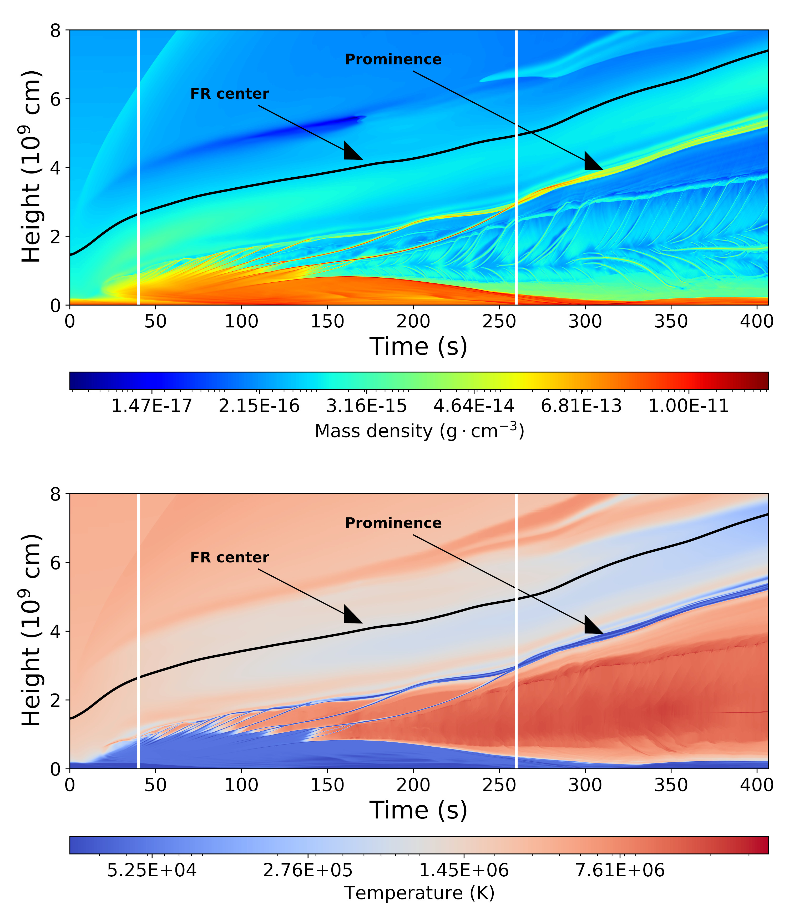
Figure 1 presents the global evolution of the thermal pressure with magnetic field lines overlaid (in grey) in the region $[-15L_{0},15L_{0}]\times[0,30L_{0}]$ while Figure 2 shows the density (first and second rows) and temperature (third and fourth rows) evolutions in a smaller region $[-3.5L_{0},3.5L_{0}]\times[0,7L_{0}]$. The chromosphere in Figure 1 manifests as a thick line at the bottom because the height of the chromosphere-corona transition region $0.2L_{0}=2\,\mathrm{Mm}$ is much smaller than $30L_{0}=300\,\mathrm{Mm}$, the size of the domain to illustrate. The chromosphere is clearly illustrated in Figure 2 where the size of the domain shown is reduced. The parameter $M_{q}$ governs the force balance of the FR as discussed in Takahashi et al. 2017 and in our Appendix. No equilibrium can be found in our setup since $M_{q}=0.8M_{c}<M_{c}$ and the FR is ejected upward immediately after the launch of the simulation due to catastrophe. Figure 3 shows the time-distance diagrams of mass density (top) and temperature (bottom) along the vertical line $x=0$ in the height range $[0,8L_{0}]$, respectively, where $L_{0}=10^{9}\,\mathrm{cm}$ is the typical length scale as listed in Table 1. The height of the FR center (the O-point) is also plotted over time in Figure 3. The kinematic evolution of the FR is divided into three phases. The FR first goes through an initial acceleration due to the non-equilibrium initial setup until $t\sim 40\,\mathrm{s}$, which is indicated by the first vertical line in Figure 3. Then the FR rises at a constant speed of $\sim 10^{7}\,\mathrm{cm\cdot s^{-1}}$ in the interval $40\,\mathrm{s}\leq t\leq 260\,\mathrm{s}$ (the region between the two vertical lines in Figure 3). The speed of the FR rise then increases from $10^{7}\,\mathrm{cm\cdot s^{-1}}$ to $\sim 3\times 10^{7}\,\mathrm{cm\cdot s^{-1}}$ after $t\sim 260\,\mathrm{s}$ as indicated by the second vertical line in Figure 3. The kinematic evolution of the FR is significantly different from what is described in Zhao et al. 2017; Zhao et al. 2019; Zhao & Keppens 2020, where the FR is formed and then undergoes a series of quasi-static equilibrium states in the initiation phase, followed by an impulsive acceleration. This difference is attributed to the different initial setups: the non-equilibrium initial setup in the current study imposes an initial acceleration to a pre-existing FR, while when an FR is formed due to converging motion, we get a quasi-static process where force balance is almost preserved in the CME initiation. In both cases though, a CS is formed underneath the FR. Below the reconnecting CS, flare loops are formed as a result of reconnection, which is consistent with the standard solar eruption model. As the reconnection continues, the flare loop system expands and its two foot-points separate. This flare foot-points separation was also reported in observations like Qiu et al. 2002 and the fully self-consistent MHD-beam flare model by Ruan et al. 2020. The fast-rising FR drives the formation of a fast-mode shock straddling over it, as shown in Figure 1 and 2. These structures expand outward continuously as the FR rises. The fast shock front is also indicated in Figure 3, which propagates at a speed of $4\times 10^{7}\,\mathrm{cm\cdot s^{-1}}$. The intersection lines between the front surface of the fast-mode shock and the chromosphere sweep the solar surface as the eruption proceeds, which may produce the Moreton waves observed in $\mathrm{H\alpha}$ wavelength (uchida1968propagation; Chen2002ApJ572L99C). This fast-mode shock in front of the FR is invoked to produce decametric-hectometric type II coronal radio bursts associated with the CME (Magara2000ApJ538L175M; Lu et al. 2017).

We now turn attention to the prominence formation and eruption aspects in the following sections.

The evolution of the mass density (first and second rows) and temperature (third and fourth rows) of the CS region is shown in Figure 2 with magnetic field lines overlaid (grey). As the FR rises, the surrounding plasma with frozen-in field lines is driven inward underneath the FR and a CS is formed, where reconnection is then triggered. The CS formation is illustrated in details in Figure 4. The bottom of the FR is buried in the chromosphere at $t=0\,\mathrm{s}$ as shown in Figure 4. The FR is ejected upward due to catastrophe as a result of the initial non-equilibrium setup. At $t=17.2\,\mathrm{s}$, the matter from the low corona is lifted up as the FR rises while the heavy chromospheric matter tries to stay in situ and deforms the bottom of the FR. As the top of the FR rises, the deformation of the bottom of the FR strengthens and leads to the formation of a CS at $t=20.6\,\mathrm{s}$. Some chromospheric matter is squeezed into the CS and is lifted by the concave-upward magnetic field lines that apply an upward Lorentz force on the chromospheric matter. The details and consequences of lifting chromospheric matter into the CS is here simulated: it can occur as long as the bottom of an erupting FR is partially buried in the chromosphere. We note that FR eruption driven by photospheric converging motions could also lift chromospheric plasma up to the CS height (Zhao et al. 2017; Zhao et al. 2019; Zhao & Keppens 2020). A previous MHD simulation of flux emergence causing eruption (Manchester et al. 2004) presented the similar magnetic evolution and the CS formation. In their simulation, the upper part of the FR emerged into the corona, while the lower part of the FR remained in the chromosphere/photosphere. As the upper part of the FR expanded in the corona (by shearing motion), the upper part and the lower part were gradually separated, forming the CS and new O-points. The CS underneath the FR extends in length and is thinning as the eruption proceeds as shown in the snapshot at $t=25.8\,\mathrm{s}$. Once the Lundquist number of the CS exceeds a critical value $S_{Lu}\simeq 10^{4}$ (Bhattacharjee et al. 2009; Huang & Bhattacharjee 2010; Shen et al. 2011; Mei et al. 2012; Zhao et al. 2021), the plasmoid-mediated fast reconnection starts, accompanied by the appearance of multiple magnetic islands in the CS as shown, e.g., in the snapshot at $171.7\,\mathrm{s}$ in Figure 2. The time-distance diagrams of mass density (top) and temperature (bottom) along the line $x=0$ are shown in Figure 3, where the CS evolution is also illustrated. In our simulation, the plasmoid instability starts at $t\sim 40\,\mathrm{s}$, which is marked by the first vertical line in Figure 3, with a Lundquist number $S_{Lu}\simeq 3.5\times 10^{4}$ of the CS. As discussed in Section III.1, the FR first goes through an initial acceleration before $t\sim 40\,\mathrm{s}$, which coincides with the instant when the plasmoid instability starts. Before this plasmoid instability starts, some cool and dense chromospheric material has been squeezed into the CS, which is seen in earlier snapshots, e.g. at $t=34.3\,\mathrm{s}$ in Figure 2 and snapshots in Figures 4. The CS regions at $t=34.3\,\mathrm{s}$ in Figure 2 are shown in a further zoomed-in view in Figures 4 and  5. As also shown in Figure 3, the CS is dense and cool before this time. The cool and dense mass in the CS is torn apart into the magnetic islands after the plasmoid instability starts. The newborn islands move upward and merge with the FR, carrying the cool and dense mass blobs into the FR. The trajectories of these islands with cool and dense matter are clearly seen in Figure 3 between the first and second vertical lines, during which the FR rises at a constant speed of $\sim 10^{7}\,\mathrm{cm\cdot s^{-1}}$.

The magnetic islands thus play a role of mass carriers of the chromospheric matter to the corona. This process is illustrated in Figure 6 in more details, where mass density (top) and temperature (bottom) in the CS region is plotted with magnetic field lines overlaid (in black). The arrows in Figure 6 indicate island A, which is a typical example to demonstrate how a magnetic island lifts the cool and dense remnant chromospheric matter in the CS into the FR. At $t=90.2\,\mathrm{s}$, island A, located in-between two adjacent islands, moves upward in the CS carrying dense and cool mass in it. At $t=103.2\,\mathrm{s}$, island A is reconnecting and coalescing with the FR. At $t=112.5\,\mathrm{s}$, island A is fully merged into the FR with its mass remaining at the bottom of the FR. As the plasmoid-mediated fast reconnection proceeds, more magnetic islands are produced and the coalescence of the islands with the FR repeats. The new-born magnetic islands successively push remnant chromospheric matter in the CS into the FR. These mass pieces are accumulated in the bottom of the FR, leading to the formation of dynamic blobs and threads. Hence we get a plasmoid-fed prominence formation or PF² process. After the second vertical line in Figure 3, the temperature and density of the islands become closer to coronal values, and the PF² process stops. Most of the islands with cool and dense mass between the first and second vertical lines move upward, while we find almost equal fractions of downward-moving and upward-moving islands consisting of hot and tenuous matter after the second vertical line, which is consistent with the findings in Zhao & Keppens 2020. The reason why most islands with cool and dense mass move upward can be seen from Figure 4, e.g., at $t=17.2\,\mathrm{s}$. The bottom of the FR is deformed by the heavy cool and dense chromospheric matter and the magnetic field lines are concave-upward. The curvature of the concave-upward magnetic field lines increases as the deformation strengthens, and meanwhile the Lorentz force increases. The Lorentz force acting upon the cool and dense matter in the newly formed CS is directed upward. The Lorentz force gives an initial upward acceleration to the cool and dense matter, and thus most islands with cool and dense matter move upward. After the cool and dense matter move away from the CS, the magnetic field lines do not have to be concave-upward and islands consisting of hot and tenuous matter formed later move both upward and downward.

Before the plasmoid instability starts, some dense and hot material from the low corona has already been injected into the FR by the reconnection outflow and accumulated at the bottom of the FR, as shown, e.g., in the snapshots at $34.3\,\mathrm{s}$ in Figure 5. This hot and dense material cools down and condenses into the newly formed prominence as the FR rises. To illustrate the entire condensation process, we plot the time profiles of the mass of the matter that is dense and cool ($\rho>2\times 10^{-15}\,\mathrm{g\cdot cm^{-3}}$ and $T<3\times 10^{5}\,\mathrm{K}$) in red, and dense and hot ($\rho>2\times 10^{-15}\,\mathrm{g\cdot cm^{-3}}$ and $T>3\times 10^{5}\,\mathrm{K}$) in green, respectively, in Figure 7. The black dashed curve represents the mass of the dense matter at any temperature, i.e., the summation of the red and green curves. Only the matter located above a height of $L_{0}=10^{9}\,\mathrm{cm}$ is counted, since dense matter below $L_{0}=10^{9}\,\mathrm{cm}$ is considered to be more closely linked to the chromosphere rather than the prominence. Figure 8 shows the density (top) and temperature (bottom) at $t=68.7\,\mathrm{s}$ and $t=214.7\,\mathrm{s}$, respectively. To illustrate the dynamically evolving regions selected to calculate the mass evolution in Figure 7, we plot black contours in Figure 8 to mark the iso-density lines ($\rho=2\times 10^{-15}\,\mathrm{g\cdot cm^{-3}}$) and red contours to represent the iso-temperature lines ($T=3\times 10^{5}\,\mathrm{K}$). The white lines represent the height $L_{0}=10^{9}\,\mathrm{cm}$. The regions above the white line and encircled by the black contours are selected to calculate the mass of the dense matter in Figure 7. The intersections of the regions encircled by the red and black contours and located above the white line constitute the dense and cool matter. Due to the two-and-a-half-dimensional setup, our system is translationally invariant in the z-direction. Therefore, to calculate the total prominence mass by an $(x,y)$-masked, 3D integral $\int_{\mathrm{mask}}\rho(x,y,t)\mathrm{d}x\mathrm{d}y\mathrm{d}z$, we artificially take the ignored z-direction as $[0,L_{0}]$, i.e., the prominence is supposed to have a length of $L_{0}=10^{9}\,\mathrm{cm}$. The red cool-and-dense curve starts to increase from $t\sim 50\,\mathrm{s}$, $10\,\mathrm{s}$ after the plasmoid instability starts, which indicates that some dense and cool chromospheric matter is lifted above $L_{0}=10^{9}\,\mathrm{cm}$ by the magnetic islands. The green curve starts to increase from an earlier instant of time $t\sim 20\,\mathrm{s}$ because the dense and hot matter exists in a higher region than the chromospheric matter and is thus lifted above the height $L_{0}=10^{9}\,\mathrm{cm}$ by the FR at an earlier time. The green curve decreases from $t\sim 68.7\,\mathrm{s}$, a few seconds after the red curve increases, which marks the beginning of the condensation. The dense and cool matter accumulated at the bottom of the FR is about $4\times 10^{11}\,\mathrm{g}$ when the condensation begins. The dense and cool matter perturbs the density and temperature distributions, triggering thermal instabilities. The hot and dense matter at the bottom of the FR continuously condenses into the newly formed prominence. The condensation process is more vividly depicted in Figure 8. The dense matter encircled by the black contours in an earlier instant $t=68.7\,\mathrm{s}$ is clearly much larger than the region encircled by the red contours (i.e., the prominence). The black contours gradually contract and finally overlay with the red contours that encircle the cool matter in the later instant $t=214.7\,\mathrm{s}$. Meanwhile, the area encircled by the red contours also grows from $t=68.7\,\mathrm{s}$ to $t=214.7\,\mathrm{s}$. This corresponds in Figure 7 to the black curve being much higher than the red curve at $t=68.7\,\mathrm{s}$, but the two curves almost overlay with each other at $t=214.7\,\mathrm{s}$, and the red curve rises from $t=68.7\,\mathrm{s}$ to $t=214.7\,\mathrm{s}$. The condensation mainly occurs in the bottom of the FR and lasts from $t\sim 68.7\,\mathrm{s}$ to $t\sim 150\,\mathrm{s}$, which falls into the time interval between the two vertical lines in Figure 7 that mark the beginning and end of the second phase of the FR eruption. Afterwards, the mass of the dense and hot matter (green curve) is ignorable and the red and black curves almost overlay with each other. Before the condensation starts from $t\sim 68.7\,\mathrm{s}$, the prominence (the dense and cool matter) formation is driven purely by the newly discovered PF² process. The mass of the prominence at $t\sim 68.7\,\mathrm{s}$ is $\sim 3\times 10^{11}\,\mathrm{g}$. After the condensation, the mass of the prominence reaches $\sim 4\times 10^{12}\,\mathrm{g}$ at $t\sim 150\,\mathrm{s}$. Although, the PF² process lasts until $t\sim 260\,\mathrm{s}$, the prominence mass keeps almost constant $\sim 4\times 10^{12}\,\mathrm{g}$ after $t\sim 150\,\mathrm{s}$ because only very few islands carry cool and dense matter to the FR and the mass gained from the PF² process after $t\sim 150\,\mathrm{s}$ is only $\sim 1\times 10^{11}\,\mathrm{g}$. The total mass gained from the condensation process is $\sim 2\times 10^{12}\,\mathrm{g}$, which is seen from the peak of the green curve, while the other half of the mass $\sim 2\times 10^{12}\,\mathrm{g}$ is from the PF² process. In early literature, Kuperus & Tandberg-Hanssen 1967 also suggested that condensation might take place in the CS and plasmoids formed by resistive instabilities would cause a filamentary thread structure in the forming prominence, as generally observed. However, their (cartoon) model is an in-situ condensation model for quiescent prominences, where the prominence mass comes from the corona by condensation. The mass transfer from the chromosphere to the corona by plasmoids, i.e., the PF² process is a new ingredient to explain eruptive prominence formations in our work.

To compare our numerical results with observations, synthesized extreme ultraviolet (EUV) radiations of the seven channels of SDO/AIA, i.e., $94\AA$, $131\AA$, $171\AA$, $193\AA$, $211\AA$, $304\AA$, and $335\AA$, are calculated based on the temperature and density obtained from the MHD simulation by forward modeling analysis. The main task of the forward modeling analysis is to calculate the radiation intensity $I_{\lambda}$ by solving the radiative transfer equation (Rybicki & Lightman 1986; Zhao et al. 2019):

where $S_{\lambda}$ is the source function and $\tau_{\lambda}$ is the optical depth. To calculate the radiation in the x-y plane, the line-of-sight integral in the radiative transfer equation is taken along the z-axis in the interval $[-5L_{0},5L_{0}]$, along which the source function $S_{\lambda}$ is constant because the system is translationally invariant due to the two-and-a-half-dimensional setup, while, in the x-z and z-y planes, i.e., the top and side views, the line-of-sight integrals are taken in the y- and x-directions in the intervals $[0,7L_{0}]$ and $[-5L_{0},5L_{0}]$, respectively, where the source function $S_{\lambda}$ is not a constant anymore. Here $L_{0}=10^{9}\,\mathrm{cm}$ is the typical length scale as listed in Table 1. The background radiation $I_{\lambda}(0)$ is taken as $1\%$ of the highest radiation value. The main technical details of our forward modeling analysis are fully described in Zhao et al. 2019.

Synthetic EUV images at $406.5\,\mathrm{s}$ of the seven channels of SDO/AIA, in the $(x,y)$ view are plotted in the top panels in Figure 9. The plasmoids are visible in the $171\AA$, $211\AA$, $304\AA$, and $335\AA$ channels, and are especially apparent in the $171\AA$ channel, which are easily identified as bright blobs. The flare loops appear bright in the $171\AA$, $211\AA$, and $304\AA$ channels. We can also identify fibril-like thread structure of the prominence in all the seven channels.

The synthetic EUV $304\AA$ images in the x-z and z-y planes, i.e., the top and side views, at the same time are also calculated and shown in the bottom-left and bottom-right panels of Figure 9, respectively. The bright flare arcade and the filament threads are clearly visible in the top and side views, as indicated by the arrows. Due to the translational invariance along the z-direction in our two-and-a-half-dimensional setup, all the filament threads are exactly oriented along the z-direction, and manifest themselves as elongated fibrils above the underlying polarity inversion line. In the recent two-dimensional simulations of an arcade-supported prominence in Zhou et al. 2020, some filament threads are found to be misaligned with the local magnetic field by $\sim 2^{\circ}$.

References

- Aly (1990) Aly, J. J. 1990, Computer Physics Communications, 59, 13, doi: 10.1016/0010-4655(90)90152-Q
- An et al. (1988) An, C.-H., Bao, J., Wu, S., & Suess, S. 1988, Solar physics, 115, 93
- Antiochos et al. (1999) Antiochos, S. K., DeVore, C. R., & Klimchuk, J. A. 1999, ApJ, 510, 485, doi: 10.1086/306563
- Antiochos et al. (1999) Antiochos, S. K., MacNeice, P. J., Spicer, D. S., & Klimchuk, J. A. 1999, The Astrophysical Journal, 512, 985
- Bárta et al. (2011) Bárta, M., Büchner, J., Karlický, M., & Skála, J. 2011, ApJ, 737, 24, doi: 10.1088/0004-637X/737/1/24
- Bhattacharjee et al. (2009) Bhattacharjee, A., Huang, Y.-M., Yang, H., & Rogers, B. 2009, Physics of Plasmas, 16, 112102, doi: 10.1063/1.3264103
- Carmichael (1964) Carmichael, H. 1964, NASA Special Publication, 50, 451
- Chen (2011) Chen, P. F. 2011, Living Reviews in Solar Physics, 8, 1, doi: 10.12942/lrsp-2011-1
- Chen & Shibata (2000) Chen, P. F., & Shibata, K. 2000, ApJ, 545, 524, doi: 10.1086/317803
- Dungey (1953) Dungey, J. 1953, The London, Edinburgh, and Dublin Philosophical Magazine and Journal of Science, 44, 725
- Fan (2018) Fan, Y. 2018, The Astrophysical Journal, 862, 54
- Forbes & Isenberg (1991) Forbes, T. G., & Isenberg, P. A. 1991, ApJ, 373, 294, doi: 10.1086/170051
- Guo et al. (2019) Guo, Q., DF, K., LH, Y., et al. 2019
- Hirayama (1974) Hirayama, T. 1974, Sol. Phys., 34, 323, doi: 10.1007/BF00153671
- Huang & Bhattacharjee (2010) Huang, Y.-M., & Bhattacharjee, A. 2010, Physics of Plasmas, 17, 062104, doi: 10.1063/1.3420208
- Illing & Hundhausen (1983) Illing, R. M. E., & Hundhausen, A. J. 1983, J. Geophys. Res., 88, 10210, doi: 10.1029/JA088iA12p10210
- Illing & Hundhausen (1985) —. 1985, J. Geophys. Res., 90, 275, doi: 10.1029/JA090iA01p00275
- Jenkins & Keppens (2021) Jenkins, J., & Keppens, R. 2021, Astronomy & Astrophysics, 646, A134
- Kaneko & Yokoyama (2017) Kaneko, T., & Yokoyama, T. 2017, The Astrophysical Journal, 845, 12
- Keppens et al. (2019) Keppens, R., Guo, Y., Makwana, K., et al. 2019, Reviews of Modern Plasma Physics, 3, 14
- Keppens et al. (2014) Keppens, R., Porth, O., & Xia, C. 2014, ApJ, 795, 77, doi: 10.1088/0004-637X/795/1/77
- Keppens et al. (2021) Keppens, R., Teunissen, J., Xia, C., & Porth, O. 2021, Computers & Mathematics with Applications, 81, 316
- Ko et al. (2003) Ko, Y.-K., Raymond, J. C., Lin, J., et al. 2003, ApJ, 594, 1068, doi: 10.1086/376982
- Kopp & Pneuman (1976) Kopp, R. A., & Pneuman, G. W. 1976, Sol. Phys., 50, 85, doi: 10.1007/BF00206193
- Kuperus & Tandberg-Hanssen (1967) Kuperus, M., & Tandberg-Hanssen, E. 1967, Solar Physics, 2, 39
- Leroy (1989) Leroy, J. 1989, Observation of Prominence Magnetic Fields, Dynamics and Structures of Quiescent Prominences, ed. ER Priest, Kluwer Academic Publishers, Dordrecht, Holland
- Lin & Forbes (2000) Lin, J., & Forbes, T. G. 2000, J. Geophys. Res., 105, 2375, doi: 10.1029/1999JA900477
- Lu et al. (2017) Lu, L., Inhester, B., Feng, L., Liu, S., & Zhao, X. 2017, ApJ, 835, 188, doi: 10.3847/1538-4357/835/2/188
- Mackay et al. (2010) Mackay, D., Karpen, J., Ballester, J., Schmieder, B., & Aulanier, G. 2010, Space Science Reviews, 151, 333
- Manchester et al. (2004) Manchester, W., I., Gombosi, T., DeZeeuw, D., & Fan, Y. 2004, ApJ, 610, 588, doi: 10.1086/421516
- Martens & Kuin (1989) Martens, P., & Kuin, N. 1989, Solar physics, 122, 263
- Mei et al. (2012) Mei, Z., Shen, C., Wu, N., et al. 2012, MNRAS, 425, 2824, doi: 10.1111/j.1365-2966.2012.21625.x
- Ni & Lukin (2018) Ni, L., & Lukin, V. S. 2018, ApJ, 868, 144, doi: 10.3847/1538-4357/aaeb97
- Ni et al. (2012) Ni, L., Roussev, I. I., Lin, J., & Ziegler, U. 2012, ApJ, 758, 20, doi: 10.1088/0004-637X/758/1/20
- Nool & Keppens (2002) Nool, M., & Keppens, R. 2002, Computational Methods in Applied Mathematics, 2, 92
- Parker (1957) Parker, E. N. 1957, J. Geophys. Res., 62, 509, doi: 10.1029/JZ062i004p00509
- Parker (1963) Parker, E. N. 1963, The Astrophysical Journal Supplement Series, 8, 177
- Petschek (1964) Petschek, H. E. 1964, NASA Special Publication, 50, 425
- Porth et al. (2014) Porth, O., Xia, C., Hendrix, T., Moschou, S. P., & Keppens, R. 2014, ApJS, 214, 4, doi: 10.1088/0067-0049/214/1/4
- Qiu et al. (2002) Qiu, J., Lee, J., Gary, D. E., & Wang, H. 2002, ApJ, 565, 1335, doi: 10.1086/324706
- Reeves et al. (2010) Reeves, K. K., Linker, J. A., Mikić, Z., & Forbes, T. G. 2010, ApJ, 721, 1547, doi: 10.1088/0004-637X/721/2/1547
- Ruan et al. (2020) Ruan, W., Xia, C., & Keppens, R. 2020, ApJ, 896, 97, doi: 10.3847/1538-4357/ab93db
- Rybicki & Lightman (1986) Rybicki, G. B., & Lightman, A. P. 1986, Radiative Processes in Astrophysics, 400
- Shen et al. (2011) Shen, C., Lin, J., & Murphy, N. A. 2011, ApJ, 737, 14, doi: 10.1088/0004-637X/737/1/14
- Shibata & Tanuma (2001) Shibata, K., & Tanuma, S. 2001, Earth, Planets, and Space, 53, 473, doi: 10.1186/BF03353258
- Spiteri & Ruuth (2002) Spiteri, R. J., & Ruuth, S. J. 2002, SIAM Journal on Numerical Analysis, 40, 469
- Sturrock (1966) Sturrock, P. A. 1966, Nature, 211, 695, doi: 10.1038/211695a0
- Sweet (1958a) Sweet, P. A. 1958a, Il Nuovo Cimento (1955-1965), 8, 188
- Sweet (1958b) Sweet, P. A. 1958b, in IAU Symposium, Vol. 6, Electromagnetic Phenomena in Cosmical Physics, ed. B. Lehnert, 123
- Takahashi et al. (2017) Takahashi, T., Qiu, J., & Shibata, K. 2017, ApJ, 848, 102, doi: 10.3847/1538-4357/aa8f97
- Titov & Démoulin (1999) Titov, V. S., & Démoulin, P. 1999, A&A, 351, 707
- Török & Kliem (2005) Török, T., & Kliem, B. 2005, ApJ, 630, L97, doi: 10.1086/462412
- Tóth & Odstrčil (1996) Tóth, G., & Odstrčil, D. 1996, Journal of Computational Physics, 128, 82, doi: 10.1006/jcph.1996.0197
- Čada & Torrilhon (2009) Čada, M., & Torrilhon, M. 2009, Journal of Computational Physics, 228, 4118, doi: 10.1016/j.jcp.2009.02.020
- Wang (1999) Wang, Y.-M. 1999, The Astrophysical Journal Letters, 520, L71
- Webb & Howard (2012) Webb, D. F., & Howard, T. A. 2012, Living Reviews in Solar Physics, 9, 3, doi: 10.12942/lrsp-2012-3
- Xia et al. (2012) Xia, C., Chen, P. F., & Keppens, R. 2012, ApJ, 748, L26, doi: 10.1088/2041-8205/748/2/L26
- Xia et al. (2011) Xia, C., Chen, P. F., Keppens, R., & van Marle, A. J. 2011, ApJ, 737, 27, doi: 10.1088/0004-637X/737/1/27
- Xia & Keppens (2016) Xia, C., & Keppens, R. 2016, ApJ, 823, 22, doi: 10.3847/0004-637X/823/1/22
- Xia et al. (2014) Xia, C., Keppens, R., Antolin, P., & Porth, O. 2014, ApJ, 792, L38, doi: 10.1088/2041-8205/792/2/L38
- Xia et al. (2018) Xia, C., Teunissen, J., El Mellah, I., Chané, E., & Keppens, R. 2018, ApJS, 234, 30, doi: 10.3847/1538-4365/aaa6c8
- Ye et al. (2020) Ye, J., Cai, Q., Shen, C., et al. 2020, ApJ, 897, 64, doi: 10.3847/1538-4357/ab93b5
- Ye et al. (2021) —. 2021, ApJ, 909, 45, doi: 10.3847/1538-4357/abdeb5
- Ye et al. (2017) Ye, J., Lin, J., Raymond, J. C., & Shen, C. 2017, in AGU Fall Meeting Abstracts, Vol. 2017, SH11B–2436
- Yee (1989) Yee, H. C. 1989
- Zhao et al. (2021) Zhao, X., Bacchini, F., & Keppens, R. 2021, Physics of Plasmas, 28, 092113, doi: 10.1063/5.0058326
- Zhao & Keppens (2020) Zhao, X., & Keppens, R. 2020, ApJ, 898, 90, doi: 10.3847/1538-4357/ab9a31
- Zhao et al. (2017) Zhao, X., Xia, C., Keppens, R., & Gan, W. 2017, ApJ, 841, 106, doi: 10.3847/1538-4357/aa7142
- Zhao et al. (2019) Zhao, X., Xia, C., Van Doorsselaere, T., Keppens, R., & Gan, W. 2019, ApJ, 872, 190, doi: 10.3847/1538-4357/ab0284
- Zhou et al. (2020) Zhou, Y., Chen, P., Hong, J., & Fang, C. 2020, Nature Astronomy, 4, 994