跳到论文正文
W Papers独立论文阅读器 arXiv:2202.08091 论文正文 计算阅读时间 · 0%
引用这篇论文根据当前论文元数据生成,正式投稿前建议核对。


License: arXiv.org perpetual non-exclusive license
arXiv:2202.08091v2 [hep-ph] 06 Oct 2022

Rare top-quark decays t→c​g​(g)t\to cg(g) in the aligned two-Higgs-doublet model

Fang-Min Cai Affiliation: Institute of Particle Physics and Key Laboratory of Quark and Lepton Physics (MOE), Central China Normal University, Wuhan, Hubei 430079, China Email: caifangmin@mails.ccnu.edu.cn    Shuichiro Funatsu Affiliation: Institute of Particle Physics and Key Laboratory of Quark and Lepton Physics (MOE), Central China Normal University, Wuhan, Hubei 430079, China Email: funatsu@mail.ccnu.edu.cn    Xin-Qiang Li Note: Corresponding author. Affiliation: Institute of Particle Physics and Key Laboratory of Quark and Lepton Physics (MOE), Central China Normal University, Wuhan, Hubei 430079, China Email: xqli@mail.ccnu.edu.cn    and Ya-Dong Yang Affiliation: Institute of Particle Physics and Key Laboratory of Quark and Lepton Physics (MOE), Central China Normal University, Wuhan, Hubei 430079, China Affiliation: School of Physics and Microelectronics, Zhengzhou University, Zhengzhou, Henan 450001, China Email: yangyd@mail.ccnu.edu.cn
Abstract

We update the Standard Model (SM) predictions for the branching ratios of the rare top-quark decays t→c​g​(g)t\to cg(g), and evaluate the maximum rates that can be reached in the aligned as well as in the four conventional two-Higgs-doublet models (2HDMs) with 𝒵2\mathcal{Z}_{2} symmetries. Taking into account the relevant constraints on the model parameters resulting from a global fit obtained at the 95.5%95.5\% confidence level, we find that the branching ratios of t→c​gt\to cg and t→c​g​gt\to cgg decays can reach up to 3.36×10−93.36\times 10^{-9} and 2.95×10−92.95\times 10^{-9} respectively, being therefore of the same order, in the aligned 2HDM (A2HDM). This is obviously different from the SM case, where the predicted branching ratio of the three-body decay t→c​g​gt\to cgg is about two orders of magnitude larger than that of the two-body decay t→c​gt\to cg. On the other hand, compared with the SM predictions, no significant enhancements are observed in the four conventional 2HDMs with 𝒵2\mathcal{Z}_{2} symmetries for the branching ratios of these two decays. Nevertheless, the predicted branching ratios of t→c​gt\to cg and t→c​g​gt\to cgg decays in the A2HDM are still out of the expected sensitivities of the future high-luminosity Large Hadron Collider and the Future Circular Collider in hadron-hadron mode.

1 Introduction

The top quark, as the heaviest elementary particle in the Standard Model (SM), can decay into other light quarks associated with gauge or scalar bosons. Among all the possible decay modes, the flavour-changing neutral-current (FCNC) decays of the top quark, which are absent at tree level and suppressed at loop level by the Glashow-Iliopoulos-Maiani (GIM) mechanism Glashow:1970gm in the SM, are very sensitive to contributions from new physics (NP) Eilam:1990zc; Deshpande:1991pn; Hou:1991un; Luke:1993cy; Atwood:1996vj; Bejar:2000ub; Diaz:2001vj; Iltan:2001yt; Arhrib:2005nx; Bar-Shalom:2005ldb; Abbas:2015cua; Hou:2020ciy; Balaji:2020qjg; Li:1993mg; deDivitiis:1997sh; Guasch:1999jp; Eilam:2001dh; Liu:2004qw; Frank:2005vd; Eilam:2006rb; Cao:2007dk; Heng:2009wr; Cao:2014udj; Dedes:2014asa; Eilam:1989zm; AguilarSaavedra:2002ns; Han:2011xd; Gao:2013fxa; Dey:2016cve; Diaz-Furlong:2016ril; Chiang:2018oyd; Altmannshofer:2019ogm; Liu:2021crr; AguilarSaavedra:2004wm; TopQuarkWorkingGroup:2013hxj. For the two-body FCNC top-quark decays t→q​Vt\to qV and t→q​ht\to qh, with q=c,uq=c,u, V=γ,Z,gV=\gamma,Z,g, and hh the SM Higgs, their branching ratios are predicted to be of the orders of 10−1710^{-17} to 10−1210^{-12} within the SM, but could be enhanced by several orders of magnitude in many NP scenarios (see, e.g., Refs. AguilarSaavedra:2004wm; TopQuarkWorkingGroup:2013hxj and references therein). Among the three-body loop-induced top-quark decays t→c​V​Vt\to cVV and t→u1​u¯2​u2t\to u_{1}\bar{u}_{2}u_{2} with ui=u,cu_{i}=u,c, the decay t→c​g​gt\to cgg has the largest branching ratio, reaching up to about 1.02×10−91.02\times 10^{-9} within the SM Diaz-Cruz:1999wcs; Cordero-Cid:2004pco; Eilam:2006uh. Interestingly, it is found that the branching ratio of the three-body decay t→c​g​gt\to cgg is about two orders of magnitude larger than that of the two-body decay t→c​gt\to cg within the SM Eilam:2006uh, a phenomenon that will be dubbed “higher-order dominance” and has also been revealed in the bottom- and charm-quark decays Hou:1988wt; Liu:1989pc; Simma:1990nr; Hou:1987vd; Hou:1990js; Greub:2000sy; Greub:1996wn. Although their SM rates are predicted to be far below the detectable level of present and future colliders, these rare FCNC top-quark decays have been widely studied in various NP models, and significant enhancements are observed relative to the SM expectations; the most prominent examples are the two-Higgs-doublet model (2HDM) Eilam:1990zc; Deshpande:1991pn; Hou:1991un; Luke:1993cy; Atwood:1996vj; Bejar:2000ub; Diaz:2001vj; Iltan:2001yt; Arhrib:2005nx; Bar-Shalom:2005ldb; Abbas:2015cua; Hou:2020ciy; Balaji:2020qjg and the supersymmetry Li:1993mg; deDivitiis:1997sh; Guasch:1999jp; Eilam:2001dh; Liu:2004qw; Frank:2005vd; Eilam:2006rb; Cao:2007dk; Heng:2009wr; Cao:2014udj; Dedes:2014asa, within which these rare top-quark decays might be even detectable at the future colliders. Especially, it is interesting to check if the “higher-order dominance” phenomenon observed in t→c​g​(g)t\to cg(g) decays within the SM Eilam:2006uh is still valid for a viable NP model.

Among the various NP scenarios, the 2HDM Lee:1973iz provides a minimal extension of the SM scalar sector by adding a second scalar doublet with hypercharge Y=1/2Y=1/2, and can naturally satisfy the electroweak precision tests, giving rise at the same time to a very rich phenomenology Gunion:1989we; Branco:2011iw. In a generic 2HDM, the non-diagonal couplings of the neutral scalars to the SM fermions would unavoidably lead to non-vanishing tree-level FCNC interactions. To avoid these unwanted tree-level FCNC couplings, an ad-hoc discrete 𝒵2\mathcal{Z}_{2} symmetry is often imposed on the Yukawa sector of the model Glashow:1976nt. Depending on the 𝒵2\mathcal{Z}_{2} charge assignments to the scalars and fermions, this results in four types of 2HDMs (types I, II, X, Y) Branco:2011iw; Gunion:1989we under the hypothesis of natural flavour conservation Glashow:1976nt. In the aligned 2HDM (A2HDM) Pich:2009sp, on the other hand, the absence of tree-level FCNC interactions is automatically guaranteed by assuming the alignment in flavour space of the two Yukawa matrices for each type of the right-handed fermions. Interestingly, the A2HDM can recover, as particular cases, all the known specific implementations of the conventional 2HDMs based on 𝒵2\mathcal{Z}_{2} symmetries. The model is also featured by possible new sources of CP violation beyond that of the Cabibbo-Kobayashi-Maskawa (CKM) quark-mixing matrix Cabibbo:1963yz; Kobayashi:1973fv. Thus, the A2HDM has been widely studied from the various theoretical points of view Ferreira:2010xe; Bijnens:2011gd; Ferreira:2015rha; Botella:2015yfa; Penuelas:2017ikk; Gori:2017qwg, as well as for its phenomenologies in the low-energy flavour physics Jung:2010ik; Jung:2010ab; Jung:2012vu; Chang:2015rva; Cho:2017jym; Cree:2011uy; Celis:2012dk; Li:2014fea; Enomoto:2015wbn; Wang:2016ggf; Hu:2016gpe; Hu:2017qxj; Arnan:2017lxi; DelleRose:2019ukt; Wang:2020kov; Eberhardt:2020dat, the electric dipole moments of the leptons, the neutron and various atoms Dekens:2014jka; Jung:2013hka; Gisbert:2019ftm; Enomoto:2021dkl, the anomalous magnetic moment of the muon Han:2015yys; Ilisie:2015tra; Han:2016bvl; Cherchiglia:2016eui; Cherchiglia:2017uwv; DelleRose:2020oaa, and the high-energy collider physics Carena:2012rw; Altmannshofer:2012ar; Bai:2012ex; Barger:2013ofa; Lopez-Val:2013yba; Wang:2013sha; Celis:2013rcs; Celis:2013ixa; Duarte:2013zfa; Ilisie:2014hea; Abbas:2015cua; Berge:2015nua; Wang:2016rvz; Ayala:2016djv; Abbas:2018pfp; Kanemura:2021atq; Ilisie:2021jek. Recently, assuming that there are no new sources of CP violation beyond the CKM quark-mixing matrix, and taking into account the most constraining processes and observables mentioned above, together with the theoretical requirements of perturbativity and positivity of the scalar potential, a detailed global fit has been performed to the A2HDM Eberhardt:2020dat.

In this paper, we shall perform a detailed study of the rare top-quark decay t→c​g​gt\to cgg and its comparison with the two-body decay t→c​gt\to cg in the A2HDM as well as in the four conventional 2HDMs with 𝒵2\mathcal{Z}_{2} symmetries. Taking into account the relevant constraints on the model parameters from a global fit obtained at the 95.5%95.5\% confidence level (CL) Eberhardt:2020dat, we find that the branching ratios of t→c​gt\to cg and t→c​g​gt\to cgg decays can reach up to 3.36×10−93.36\times 10^{-9} and 2.95×10−92.95\times 10^{-9} respectively, being therefore of the same order, in the A2HDM. This is obviously different from the SM case, where the predicted branching ratio of t→c​g​gt\to cgg is about two orders of magnitude larger than that of t→c​gt\to cg Eilam:2006uh. On the other hand, compared with the SM predictions, no significant enhancements are observed in the four conventional 2HDMs with 𝒵2\mathcal{Z}_{2} symmetries for the branching ratios of these two decays. Searches for the decay t→c​gt\to cg have been performed at the Large Hadron Collider (LHC), with the upper limit on its branching ratio being of 𝒪⁡(10−4)\mathcal{O}(10^{-4}) ATLAS:2015iqc; CMS:2016uzc, which is still much higher than the model predictions. These rare FCNC decays will also be studied at the future experiments, such as the high-luminosity LHC (HL-LHC) Azzi:2019yne; Cepeda:2019klc; CidVidal:2018eel; Cerri:2018ypt; Atlas:2019qfx and the Future Circular Collider (FCC) Abada:2019lih; Abada:2019zxq; Benedikt:2018csr; Abada:2019ono. For example, the 95%95\%-CL limit on the branching ratio of t→c​gt\to cg at the 100100-TeV\mathrm{TeV} FCC in hadron-hadron mode (FCC-hh) with an integrated luminosity of 10​ab−110~\text{ab}^{-1} is estimated to be of 𝒪⁡(10−7−10−8)\mathcal{O}(10^{-7}-10^{-8}) Oyulmaz:2019jqr; Khanpour:2019qnw, which is at least one order of magnitude higher than the maximum value predicted in the A2HDM. As a consequence, the predicted branching ratios of t→c​gt\to cg and t→c​g​gt\to cgg decays in the A2HDM are still out of the expected sensitivities of the future HL-LHC and FCC-hh.

This paper is organized as follows. In Section 2, we recapitulate the A2HDM, focusing only on the scalar and Yukawa sectors that are most relevant to us. In Section 3, we present our calculation of the decay rates of t→c​g​(g)t\to cg(g) decays, with the resulting RR functions present in the t→c​g​gt\to cgg decay supplemented in Appendix A. Our numerical results are then given in Section 4, where we show the maximum branching ratios of t→c​g​(g)t\to cg(g) decays that can be reached in the A2HDM, and give also a simple analysis of these two decays in the four conventional 2HDMs with 𝒵2\mathcal{Z}_{2} symmetries. Our conclusion is finally made in Section 5.

2 Aligned two-Higgs-doublet model

As a simple extension of the SM, the 2HDM is invariant under the SM gauge group and includes, besides the SM matter and gauge fields, two complex scalar S​U​(2)LSU(2)_{L} doublets,

ϕa=ei​θa​[ϕa+12​(va+ρa+i​ηa)],\phi_{a}=\mathrm{e}^{i\theta_{a}}\left[\begin{array}[]{c}\phi_{a}^{+}\\[4.26773pt] \frac{1}{\sqrt{2}}\left(v_{a}+\rho_{a}+i\eta_{a}\right)\end{array}\right]\,, (1)

with the weak hypercharge Y=1/2Y=1/2. Here we have assumed that the vacuum of the theory respects the electromagnetic gauge symmetry, which guarantees the vacuum expectation values (vevs) of the two scalar fields ϕa\phi_{a} to be aligned in the S​U​(2)LSU(2)_{L} space. After performing further a global S​U​(2)LSU(2)_{L} transformation to put the non-zero vevs only in the lower (neutral) components of ϕa\phi_{a}, which guarantees the vacuum to be neutral and not charge-breaking, we can bring the vevs of the two scalar fields to the forms given by ⟨0|ϕaT​(x)|0⟩=(0,va​ei​θa/2)\langle 0|\phi_{a}^{T}(x)|0\rangle=(0,v_{a}e^{i\theta_{a}}/\sqrt{2}), where v1v_{1} and v2v_{2} are real and non-negative Ginzburg:2004vp; Davidson:2005cw. However, as one global phase can always be rotated away through an appropriate U​(1)YU(1)_{Y} transformation, we can, without loss of generality, fix θ1=0\theta_{1}=0 and leave the relative phase θ=θ2−θ1\theta=\theta_{2}-\theta_{1} Ginzburg:2004vp; Davidson:2005cw; Pich:2009sp.

Performing further a global S​U​(2)SU(2) transformation in the scalar space (ϕ1,ϕ2)(\phi_{1},\phi_{2}), we can rotate the original scalar basis to the so-called Higgs basis Davidson:2005cw; Haber:2006ue; Haber:2010bw; Botella:1994cs,

(Φ1−Φ2)≡(cos⁡βsin⁡βsin⁡β−cos⁡β)​(ϕ1e−i​θ​ϕ2),\left(\begin{array}[]{c}\Phi_{1}\\[2.84544pt] -\Phi_{2}\end{array}\right)\equiv\left(\begin{array}[]{cc}\cos\beta&\sin\beta\\[4.26773pt] \sin\beta&-\cos\beta\end{array}\right)\,\left(\begin{array}[]{c}\phi_{1}\\[2.84544pt] \mathrm{e}^{-i\theta}\phi_{2}\end{array}\right)\;, (2)

where the rotation angle β\beta is defined by the ratio of the absolute values of the two neutral scalar field vevs, tan⁡β≡|⟨0|ϕ20|0⟩||⟨0|ϕ10|0⟩|=v2v1\tan\beta\equiv\frac{\left|\left\langle 0|\phi_{2}^{0}\right|0\rangle\right|}{\left|\left\langle 0|\phi_{1}^{0}\right|0\rangle\right|}=\frac{v_{2}}{v_{1}}, and, by convention, its value is limited to the first quadrant due to v1,v2≥0v_{1},v_{2}\geq 0. In fact, both tan⁡β\tan\beta and the relative phase θ\theta are basis-dependent, and we can remove them entirely by transforming from a generic basis (ϕ1,ϕ2)(\phi_{1},\phi_{2}) to the Higgs basis (Φ1,Φ2)(\Phi_{1},\Phi_{2}) Davidson:2005cw; Haber:2006ue; Haber:2010bw; Botella:1994cs. The true significance of tan⁡β\tan\beta emerges only in specialized versions of the 2HDM, such as the four conventional 2HDMs with 𝒵2\mathcal{Z}_{2} symmetries, where tan⁡β\tan\beta is promoted to a physical parameter. In this case, we can remove the relative phase θ\theta by making a phase rotation ϕ2→e−i​θ​ϕ2\phi_{2}\to\mathrm{e}^{-i\theta}\phi_{2}, such that the two neutral scalar vevs are real and the CP invariance is not spontaneously broken Davidson:2005cw; Haber:2006ue; Haber:2010bw; Botella:1994cs. In the Higgs basis, only the scalar doublet Φ1\Phi_{1} gets a non-zero vev, ⟨0|Φ1T​(x)|0⟩=(0,v/2)\langle 0|\Phi_{1}^{T}\left(x\right)|0\rangle=(0,v/\sqrt{2}), with v=v12+v22=1/2​GF≃246.22​GeVv=\sqrt{v_{1}^{2}+v_{2}^{2}}=1/\sqrt{\sqrt{2}G_{F}}\simeq 246.22\,{\rm GeV}, and plays the role of the SM Higgs doublet. The two scalar doublets in the Higgs basis can now be parametrized, respectively, as Pich:2009sp

Φ1=[G+12​(v+S1+i​G0)],Φ2=[H+12​(S2+i​S3)],\Phi_{1}=\left[\begin{array}[]{c}G^{+}\\[4.26773pt] \frac{1}{\sqrt{2}}\,(v+S_{1}+iG^{0})\end{array}\right]\;,\qquad\Phi_{2}=\left[\begin{array}[]{c}H^{+}\\[4.26773pt] \frac{1}{\sqrt{2}}\,(S_{2}+iS_{3})\end{array}\right]\;, (3)

where G±G^{\pm} and G0G^{0} denote the electroweak Goldstone fields, and the remaining five physical degrees of freedom are given by the two charged fields H±​(x)H^{\pm}(x) and the three neutral ones φi0​(x)={h⁡(x),H⁡(x),A⁡(x)}=ℛi​j​Sj\varphi^{0}_{i}(x)=\{h(x),H(x),A(x)\}=\mathcal{R}_{ij}S_{j}, where ℛ\mathcal{R} is the orthogonal matrix needed for diagonalizing the mass terms in the scalar potential Celis:2013rcs. Generally, none of these three neutral scalars can have a definite CP quantum number. Here, for simplicity, we shall assume a CP-conserving Higgs sector, as will be detailed in the next two subsections.

2.1 Scalar sector

In the Higgs basis, the most general scalar potential allowed by the electroweak gauge symmetry S​U​(2)L⊗U​(1)YSU(2)_{L}\otimes U(1)_{Y} takes the form Davidson:2005cw; Haber:2006ue; Haber:2010bw:

V\displaystyle V =μ1​(Φ1†​Φ1)+μ2​(Φ2†​Φ2)+[μ3​(Φ1†​Φ2)+μ3∗​(Φ2†​Φ1)]\displaystyle=\mu_{1}\,\left(\Phi_{1}^{\dagger}\Phi_{1}\right)\,+\,\mu_{2}\,\left(\Phi_{2}^{\dagger}\Phi_{2}\right)\,+\,\left[\mu_{3}\,\left(\Phi_{1}^{\dagger}\Phi_{2}\right)\,+\,\mu_{3}^{*}\,\left(\Phi_{2}^{\dagger}\Phi_{1}\right)\right]
+λ1​(Φ1†​Φ1)2+λ2​(Φ2†​Φ2)2+λ3​(Φ1†​Φ1)​(Φ2†​Φ2)+λ4​(Φ1†​Φ2)​(Φ2†​Φ1)\displaystyle+\lambda_{1}\,\left(\Phi_{1}^{\dagger}\Phi_{1}\right)^{2}\,+\,\lambda_{2}\,\left(\Phi_{2}^{\dagger}\Phi_{2}\right)^{2}\,+\,\lambda_{3}\,\left(\Phi_{1}^{\dagger}\Phi_{1}\right)\left(\Phi_{2}^{\dagger}\Phi_{2}\right)\,+\,\lambda_{4}\,\left(\Phi_{1}^{\dagger}\Phi_{2}\right)\left(\Phi_{2}^{\dagger}\Phi_{1}\right)
+[(λ5Φ1†Φ2+λ6Φ1†Φ1+λ7Φ2†Φ2)(Φ1†Φ2)+h.c.].\displaystyle+\left[\left(\lambda_{5}\,\Phi_{1}^{\dagger}\Phi_{2}\,+\,\lambda_{6}\,\Phi_{1}^{\dagger}\Phi_{1}\,+\,\lambda_{7}\,\Phi_{2}^{\dagger}\Phi_{2}\right)\left(\Phi_{1}^{\dagger}\Phi_{2}\right)\,+\,\mathrm{h.c.}\right]\,. (4)

Due to Hermiticity of the scalar potential, the parameters μ1,2\mu_{1,2} and λ1,2,3,4\lambda_{1,2,3,4} are real, while μ3\mu_{3} and λ5,6,7\lambda_{5,6,7} could be generally complex. The minimization condition of the scalar potential imposes the relations

μ1=−λ1​v2,μ3=−12​λ6​v2.\displaystyle\mu_{1}=-\lambda_{1}\,v^{2},\qquad\mu_{3}=-\frac{1}{2}\,\lambda_{6}\,v^{2}. (5)

Inserting Eq. (3) into Eq. (2.1) and imposing the minimization condition given by Eq. (5), we can get the charged-Higgs mass

mH±2=μ2+12​λ3​v2,\displaystyle m_{H^{\pm}}^{2}=\mu_{2}+\frac{1}{2}\lambda_{3}\,v^{2}, (6)

while the masses of the three neutral scalars can be obtained after diagonalizing the mass-squared matrix ℳ\mathcal{M} of the three neutral-scalar fields S1,2,3S_{1,2,3} by the orthogonal matrix ℛ\mathcal{R}, i.e., diag⁡(mh2,mH2,mA2)=ℛ​ℳ​ℛT\mathrm{diag}\left(m_{h}^{2},m_{H}^{2},m_{A}^{2}\right)=\mathcal{R}\,\mathcal{M}\,\mathcal{R}^{T} Celis:2013rcs. In the CP-conserving limit of the scalar potential, the parameters λ5,6,7\lambda_{5,6,7} are all real and the three neutral scalars hh, HH, and AA are therefore CP eigenstates. In this case, the CP-odd scalar AA corresponds to the field S3S_{3}, while the two CP-even scalars hh and HH are the orthogonal combinations of S1S_{1} and S2S_{2}:

(hH)=(cos⁡α~sin⁡α~−sin⁡α~cos⁡α~)​(S1S2),\displaystyle\left(\begin{array}[]{c}h\\[2.84544pt] H\end{array}\right)\;=\;\left(\begin{array}[]{cc}\cos{\tilde{\alpha}}&\sin{\tilde{\alpha}}\\[4.26773pt] -\sin{\tilde{\alpha}}&\cos{\tilde{\alpha}}\end{array}\right)\;\left(\begin{array}[]{c}S_{1}\\[2.84544pt] S_{2}\end{array}\right)\,,

where the mixing angle α~\tilde{\alpha} is determined by

tan⁡α~=mh2−2​λ1​v2v2​λ6=v2​λ62​λ1​v2−mH2.\tan{\tilde{\alpha}}\;=\;\frac{m_{h}^{2}-2\lambda_{1}v^{2}}{v^{2}\lambda_{6}}\;=\;\frac{v^{2}\lambda_{6}}{2\lambda_{1}v^{2}-m_{H}^{2}}\,. (13)

Note that one can always restrict α~\tilde{\alpha} within the range 0⩽α~<π0\leqslant\tilde{\alpha}<\pi by performing a phase redefinition of the two CP-even fields S1S_{1} and S2S_{2}. In addition, the masses of hh and HH satisfy the relation mH2​sin2⁡α~+mh2​cos2⁡α~=2​λ1​v2m_{H}^{2}\sin^{2}{\tilde{\alpha}}+m_{h}^{2}\cos^{2}{\tilde{\alpha}}=2\lambda_{1}v^{2} Celis:2013ixa, which, together with our convention mh≤mHm_{h}\leq m_{H}, implies that 2​λ1​v2−mH2≤02\lambda_{1}v^{2}-m_{H}^{2}\leq 0 and mh2−2​λ1​v2≤0m_{h}^{2}-2\lambda_{1}v^{2}\leq 0. Then, from Eq. (13), one can see that the sign of tan⁡α~\tan{\tilde{\alpha}} is uniquely determined by that of the parameter λ6\lambda_{6}, since the vev v=v12+v22v=\sqrt{v_{1}^{2}+v_{2}^{2}} is, by definition, always positive. As the Higgs basis of a CP-conserving 2HDM is defined up to a global rephasing of the second scalar doublet Φ2→ei​η​Φ2\Phi_{2}\to\mathrm{e}^{i\eta}\Phi_{2}, we can use this freedom to change the sign of λ6\lambda_{6} ONeil:2009fty. Here, without loss of generality, we shall use the rephasing Φ2→−Φ2\Phi_{2}\to-\Phi_{2} to fix λ6⩽0\lambda_{6}\leqslant 0 so that tan⁡α~≥0\tan{\tilde{\alpha}}\geq 0, which, together with 0⩽α~<π0\leqslant\tilde{\alpha}<\pi, results in our final choice 0⩽α~⩽π/20\leqslant\tilde{\alpha}\leqslant\pi/2. The masses of the three neutral scalars are finally given, respectively, by

mh2=12​(Σ−Δ),mH2=12​(Σ+Δ),mA2=mH±2+v2​(λ42−λ5),\displaystyle m_{h}^{2}=\frac{1}{2}(\Sigma-\Delta),\qquad m_{H}^{2}=\frac{1}{2}(\Sigma+\Delta),\qquad m_{A}^{2}=m_{H^{\pm}}^{2}+v^{2}\left(\frac{\lambda_{4}}{2}-\lambda_{5}\right), (14)

with

Σ=mH±2+v2​(2​λ2+λ42−λ5),\displaystyle\Sigma=m_{H^{\pm}}^{2}+v^{2}\,\left(2\lambda_{2}+\frac{\lambda_{4}}{2}-\lambda_{5}\right), (15)
Δ=[mA2+2​v2​(λ5−λ1)]2+4​v4​λ62.\displaystyle\Delta=\sqrt{\left[m_{A}^{2}+2v^{2}\,(\lambda_{5}-\lambda_{1})\right]^{2}+4v^{4}\,\lambda_{6}^{2}}. (16)

Here the convention mh⩽mHm_{h}\leqslant m_{H} has been chosen, and the SM limit is recovered when α~=0\tilde{\alpha}=0.

2.2 Yukawa sector

The Yukawa Lagrangian of a 2HDM in the Higgs basis can be written as Pich:2009sp; Branco:2011iw

ℒY,weak=\displaystyle\mathcal{L}_{Y,\text{weak}}= −2v[Q¯L′(Md′Φ1+Yd′Φ2)dR′+Q¯L′(Mu′Φ~1+Yu′Φ~2)uR′\displaystyle-\frac{\sqrt{2}}{v}\,\Big[\bar{Q}^{\prime}_{L}(M^{\prime}_{d}\Phi_{1}+Y^{\prime}_{d}\Phi_{2})d^{\prime}_{R}+\bar{Q}^{\prime}_{L}(M^{\prime}_{u}\tilde{\Phi}_{1}+Y^{\prime}_{u}\tilde{\Phi}_{2})u^{\prime}_{R}
+L¯L′(Mℓ′Φ1+Yℓ′Φ2)ℓR′]+h.c.\displaystyle\quad\quad\,\,+\bar{L}^{\prime}_{L}(M^{\prime}_{\ell}\Phi_{1}+Y^{\prime}_{\ell}\Phi_{2})\ell^{\prime}_{R}\Big]+\mathrm{h.c.} (17)

Here, QL′Q_{L}^{\prime} and LL′L_{L}^{\prime} are the left-handed quark and lepton doublets, while uR′u^{\prime}_{R}, dR′d^{\prime}_{R}, ℓR′\ell^{\prime}_{R} denote the right-handed fermion singlets, all being given in the weak-interaction basis; Φ~a​(x)≡i​σ2​Φa∗​(x)\tilde{\Phi}_{a}(x)\equiv i\sigma_{2}\Phi_{a}^{\ast}(x), with σ2\sigma_{2} the Pauli matrix, are the charge-conjugated fields with hypercharge Y=−1/2Y=-1/2; Mf′M^{\prime}_{f} (f=u,d,ℓf=u,d,\ell) denote the non-diagonal matrices that encode both the fermion masses and the Yukawa couplings of the scalar doublet Φ1\Phi_{1} to fermions, while Yf′Y^{\prime}_{f} characterize only the Yukawa couplings of the second doublet Φ2\Phi_{2} to fermions.

In general, the two matrices Mf′M^{\prime}_{f} and Yf′Y^{\prime}_{f} associated with the same type of right-handed fermion uR′u^{\prime}_{R}, dR′d^{\prime}_{R}, or ℓR′\ell^{\prime}_{R} in Eq. (2.2) cannot be simultaneously diagonalized in flavour space. As a consequence, in the fermion mass-eigenstate basis with diagonal mass matrices Mf=ULf†M′fURfM_{f}=U_{L}^{f\dagger}M^{\prime}_{f}U_{R}^{f}, the corresponding Yukawa matrices Yf=ULf†Y′fURfY_{f}=U_{L}^{f\dagger}Y^{\prime}_{f}U_{R}^{f} remain still non-diagonal and hence give rise to non-vanishing tree-level FCNC interactions. These unwanted tree-level FCNC couplings can, however, be eliminated by requiring that the two matrices Mf′M^{\prime}_{f} and Yf′Y^{\prime}_{f} are aligned in flavour space Pich:2009sp. This results in the following alignment relations between the mass and the Yukawa matrices Pich:2009sp:

Yd,ℓ=ςd,ℓ​Md,ℓ,Yu=ςu∗​Mu,Y_{d,\ell}=\varsigma_{d,\ell}\,M_{d,\ell},\qquad Y_{u}=\varsigma_{u}^{*}\,M_{u}, (18)

where ςf\varsigma_{f} are arbitrary complex parameters and could introduce new sources of CP violation beyond that of the CKM quark-mixing matrix. They are also scalar-basis independent and satisfy universality among the three different generations Pich:2009sp.

In terms of the fermion mass eigenstates, fL,R=UL,Rf†fL,R′f_{L,R}=U_{L,R}^{f\dagger}f_{L,R}^{\prime}, and making use of the alignment conditions specified by Eq. (18), we can finally rewrite the Yukawa Lagrangian of the A2HDM as Pich:2009sp

ℒY,mass=\displaystyle\mathcal{L}_{Y,\text{mass}}= −i​G0v​{d¯L​Md​dR+u¯R​Mu†​uL+ℓ¯L​Mℓ​ℓR}\displaystyle-i\frac{G^{0}}{v}\Big\{\bar{d}_{L}M_{d}d_{R}+\bar{u}_{R}M_{u}^{\dagger}u_{L}+\bar{\ell}_{L}M_{\ell}\ell_{R}\Big\}
−(1+S1v)​{u¯L​Mu​uR+d¯L​Md​dR+ℓ¯L​Mℓ​ℓR}\displaystyle-\left(1+\frac{S_{1}}{v}\right)\Big\{\bar{u}_{L}M_{u}u_{R}+\bar{d}_{L}M_{d}d_{R}+\bar{\ell}_{L}M_{\ell}\ell_{R}\Big\}
−1v​(S2+i​S3)​{d¯L​Yd​dR+u¯R​Yu†​uL+ℓ¯L​Yℓ​ℓR}\displaystyle-\frac{1}{v}\left(S_{2}+iS_{3}\right)\Big\{\bar{d}_{L}Y_{d}d_{R}+\bar{u}_{R}Y_{u}^{\dagger}u_{L}+\bar{\ell}_{L}Y_{\ell}\ell_{R}\Big\}
−2v​G+​{u¯L​VCKM​Md​dR−u¯R​Mu†​VCKM​dL+ν¯L​Mℓ​ℓR}\displaystyle-\frac{\sqrt{2}}{v}G^{+}\Big\{\bar{u}_{L}V_{\mathrm{CKM}}M_{d}d_{R}-\bar{u}_{R}M_{u}^{\dagger}V_{\mathrm{CKM}}d_{L}+\bar{\nu}_{L}M_{\ell}\ell_{R}\Big\}
−2v​H+​{ςd​u¯L​VCKM​Md​dR−ςu​u¯R​Mu†​VCKM​dL+ςℓ​ν¯L​Mℓ​ℓR}+h.c.,\displaystyle-\frac{\sqrt{2}}{v}H^{+}\Big\{\varsigma_{d}\,\bar{u}_{L}V_{\mathrm{CKM}}M_{d}d_{R}-\varsigma_{u}\,\bar{u}_{R}M_{u}^{\dagger}V_{\mathrm{CKM}}d_{L}+\varsigma_{\ell}\,\bar{\nu}_{L}M_{\ell}\ell_{R}\Big\}+\mathrm{h.c.}\,, (19)

where VCKM=ULu†ULdV_{\text{CKM}}=U_{L}^{u\dagger}U_{L}^{d} is the usual CKM matrix Cabibbo:1963yz; Kobayashi:1973fv, and the diagonal fermion mass matrices are now given, respectively, by

Mu=diag⁡(mu,mc,mt),Md=diag⁡(md,ms,mb),Mℓ=diag⁡(me,mμ,mτ).\displaystyle M_{u}=\mathrm{diag}\left(m_{u},m_{c},m_{t}\right),\quad M_{d}=\mathrm{diag}\left(m_{d},m_{s},m_{b}\right),\quad M_{\ell}=\mathrm{diag}\left(m_{e},m_{\mu},m_{\tau}\right)\,. (20)

For the rare FCNC decays t→c​g​(g)t\to cg(g) considered here, besides the SM part, only the interactions of the charged scalars H±H^{\pm} with the quarks are involved, which means that only the alignment parameters ςu,d\varsigma_{u,d} and the charged-Higgs mass mH±m_{H^{\pm}} will be involved throughout this work.

Model ςd\varsigma_{d} ςu\varsigma_{u} ςℓ\varsigma_{\ell}
Type I cot⁡β\cot{\beta} cot⁡β\cot{\beta} cot⁡β\cot{\beta}
Type II −tan⁡β-\tan{\beta} cot⁡β\cot{\beta} −tan⁡β-\tan{\beta}
Type X cot⁡β\cot{\beta} cot⁡β\cot{\beta} −tan⁡β-\tan{\beta}
Type Y −tan⁡β-\tan{\beta} cot⁡β\cot{\beta} cot⁡β\cot{\beta}
Table 1: The one-to-one correspondence between the different choices of the alignment parameters ςf\varsigma_{f} and the four conventional 2HDMs based on discrete 𝒵2\mathcal{Z}_{2} symmetries.

As shown in Table 1, the four conventional 2HDMs Branco:2011iw; Gunion:1989we based on discrete 𝒵2\mathcal{Z}_{2} symmetries can be easily recovered from the A2HDM by choosing particular values of the alignment parameters ςf\varsigma_{f}. As the parameter ςℓ\varsigma_{\ell} is not involved in the rare decays t→c​g​(g)t\to cg(g), we are actually left with only two cases, type-I (type-X) 2HDM with ςd=ςu=cot⁡β\varsigma_{d}=\varsigma_{u}=\cot{\beta}, and type-II (type-Y) 2HDM with ςd=−1/ςu=−tanβ\varsigma_{d}=-1/\varsigma_{u}=-\tan{\beta}. Numerical results of the branching ratios of t→c​g​(g)t\to cg(g) decays in these two specific cases as well as their comparisons with the SM predictions and the results obtained in the A2HDM will also be discussed in Section 4.

3 Calculation of the decay rates

3.1 General remarks

The rare top-quark decays t→q​g​(g)t\to qg(g), with q=u,cq=u,c, occur firstly at one-loop level within the SM. As such, the decay rates of these processes are not only suppressed by the loop factor, but also receive a strong CKM and GIM suppression relative to the dominant tree-level decay t→b​W+t\to bW^{+} Eilam:1990zc; AguilarSaavedra:2002ns; Eilam:2006uh. Due to the additional charged-Higgs contributions at the loop level, however, these decay rates could be enhanced in the A2HDM as well as in the conventional 2HDMs with 𝒵2\mathcal{Z}_{2} symmetries Eilam:1990zc; Deshpande:1991pn; Bejar:2000ub. Here we shall focus on the decays into a charm instead of an up quark, because the decay rates of t→u​g​(g)t\to ug(g) are further suppressed by the ratio |Vu​b/Vc​b|2≃0.0087|V_{ub}/V_{cb}|^{2}\simeq 0.0087 compared to that of t→c​g​(g)t\to cg(g), both within the SM as well as in the 2HDMs considered.

Within the SM, due to the hierarchy of the CKM matrix elements, |Vt​b|≫|Vt​d|,|Vt​s||V_{tb}|\gg|V_{td}|,|V_{ts}|, the total width of the top quark is dominated by the tree-level two-body decay t→b​W+t\to bW^{+}, and we can, therefore, take the approximation Γtot​(t)≃Γ⁡(t→b​W+)\Gamma_{\mathrm{tot}}(t)\simeq\Gamma(t\to bW^{+}). Keeping only the dominant next-to-leading-order (NLO) QCD correction Jezabek:1988iv; Czarnecki:1990kv; Li:1990qf while neglecting the WW-boson width effect Jezabek:1988iv, the NLO electroweak Denner:1990ns; Eilam:1991iz, as well as the next-to-next-to-leading-order QCD correction Brucherseifer:2013iv; Gao:2012ja; Blokland:2004ye; Chetyrkin:1999ju; Czarnecki:1998qc, all being only of a few percentages of the Born term Gao:2012ja, we can write the partial decay width of the channel t→b​W+t\to bW^{+} as Li:1990qf; Eilam:1991iz

Γ⁡(t→b​W+)\displaystyle\Gamma(t\to bW^{+}) =\displaystyle= Γ0(t→bW+){1+CF​αs2​π[ 2(1−βW2)​(2​βW2−1)​(βW2−2)βW4​(3−2​βW2)ln(1−βW2)\displaystyle\Gamma_{0}(t\to bW^{+})\Biggl\{1+\frac{C_{F}\alpha_{s}}{2\pi}\left[\,2\frac{(1-\beta_{W}^{2})(2\beta_{W}^{2}-1)(\beta_{W}^{2}-2)}{\beta_{W}^{4}(3-2\beta_{W}^{2})}\ln(1-\beta_{W}^{2})\right. (21)
−9−4​βW23−2​βW2lnβW2+2Li2(βW2)−2Li2(1−βW2)−6​βW4−3​βW2−82​βW2​(3−2​βW2)−π2]},\displaystyle\hskip-34.14322pt\left.-\frac{9-4\beta_{W}^{2}}{3-2\beta_{W}^{2}}\ln\beta_{W}^{2}+2\mathrm{Li}_{2}(\beta_{W}^{2})-2\mathrm{Li}_{2}(1-\beta_{W}^{2})-\frac{6\beta_{W}^{4}-3\beta_{W}^{2}-8}{2\beta_{W}^{2}(3-2\beta_{W}^{2})}-\pi^{2}\,\right]\Biggr\},

where CF=4/3C_{F}=4/3 is the colour factor, and αs=gs2/(4​π)\alpha_{s}=g_{s}^{2}/(4\pi) denotes the strong coupling constant. The parameter βW=1−mW2/mt2\beta_{W}=\sqrt{1-m_{W}^{2}/m_{t}^{2}}, with mWm_{W} and mtm_{t} the WW-boson and the top-quark mass respectively, is the velocity of W+W^{+} in the top-quark rest frame, and the dilogarithm function is defined by Li2(x)=−∫0xln(1−t)/tdt\mbox{Li}_{2}(x)=-\int_{0}^{x}\text{ln}(1-t)/t\,dt. The leading-order (LO) decay width Γ0​(t→b​W+)\Gamma_{0}(t\to bW^{+}) in Eq. (21) is given by Denner:1990ns

Γ0​(t→b​W+)=GF​|Vt​b|2​λ⁡(mt,mb,mW)8​π​2​mt3​[(mt2−mb2)2+(mt2+mb2)​mW2−2​mW4],\displaystyle\Gamma_{0}(t\to bW^{+})=\frac{G_{F}|V_{tb}|^{2}\sqrt{\lambda(m_{t},m_{b},m_{W})}}{8\pi\sqrt{2}\,m_{t}^{3}}\Big[(m_{t}^{2}-m_{b}^{2})^{2}+(m_{t}^{2}+m_{b}^{2})m_{W}^{2}-2m_{W}^{4}\Big], (22)

where GFG_{F} is the Fermi constant, mbm_{b} the bottom-quark mass, and λ⁡(x,y,z)=(x2−y2−z2)2−4​y2​z2\lambda(x,y,z)=(x^{2}-y^{2}-z^{2})^{2}-4y^{2}z^{2} the usual triangle (or Källén) function for a two-body decay.

To a very good approximation, Γtot​(t)≃Γ⁡(t→b​W+)\Gamma_{\mathrm{tot}}(t)\simeq\Gamma(t\to bW^{+}) holds also in the A2HDM as well as in the four conventional 2HDMs with 𝒵2\mathcal{Z}_{2} symmetries, except when mH±<mt−mbm_{H^{\pm}}<m_{t}-m_{b}; in this regime, the top quark can have an appreciable chance to decay into the final state b​H+bH^{+}, which must be taken into account for the total top width. In this case, we shall have Γtot​(t)≃Γ⁡(t→b​W+)+Γ⁡(t→b​H+)\Gamma_{\mathrm{tot}}(t)\simeq\Gamma(t\to bW^{+})+\Gamma(t\to bH^{+}), with the LO partial width of the decay t→b​H+t\to bH^{+} in the A2HDM given by Abbas:2015cua

Γ⁡(t→b​H+)\displaystyle\Gamma(t\to bH^{+}) =\displaystyle= GF​|Vt​b|2​λ⁡(mt,mb,mH±)8​π​2​mt3[(mt2+mb2−mH±2)(mb2|ςd|2+mt2|ςu|2)\displaystyle\frac{G_{F}|V_{tb}|^{2}\sqrt{\lambda(m_{t},m_{b},m_{H^{\pm}})}}{8\pi\sqrt{2}\,m_{t}^{3}}\Big[\left(m_{t}^{2}+m_{b}^{2}-m_{H^{\pm}}^{2}\right)\left(m_{b}^{2}|\varsigma_{d}|^{2}+m_{t}^{2}|\varsigma_{u}|^{2}\right) (23)
−4mb2mt2Re(ςdςu∗)].\displaystyle\hskip 142.26378pt-4m_{b}^{2}m_{t}^{2}\,\mathrm{Re}(\varsigma_{d}\varsigma_{u}^{*})\,\Big].

As we are primarily interested in checking if the “higher-order dominance” phenomenon observed in t→c​g​(g)t\to cg(g) decays within the SM Eilam:2006uh is still valid for the A2HDM and the four conventional 2HDMs with 𝒵2\mathcal{Z}_{2} symmetries, the charged-Higgs mass mH±m_{H^{\pm}} will be assumed to be larger than the top-quark mass mtm_{t}, and the decay mode t→b​H+t\to bH^{+} is therefore kinematically forbidden. Thus, the branching ratios of t→c​g​(g)t\to cg(g) decays can be defined as

ℬ⁡(t→c​g​(g))=Γ⁡(t→c​g​(g))Γ⁡(t→b​W+).\mathcal{B}(t\to cg(g))=\frac{\Gamma(t\to cg(g))}{\Gamma(t\to bW^{+})}\,. (24)

In the next two subsections, we shall detail the calculation of the decay rates Γ⁡(t→c​g​(g))\Gamma(t\to cg(g)) in the A2HDM. To this end, we shall follow the following procedure: Firstly, we implement the A2HDM into the Mathematica-based package FeynRules Christensen:2008py; Alloul:2013bka to generate the model file together with a complete set of Feynman rules, which is then fed into the package FeynArts Kublbeck:1990xc; Hahn:2000kx to generate the one-loop Feynman diagrams and the corresponding amplitudes for the t→c​g​(g)t\to cg(g) decays. Then, we resort to the packages FormCalc Hahn:1998yk; Hahn:1999mt and LoopTools Hahn:1998yk to manipulate the decay amplitudes and evaluate numerically the scalar and tensor one-loop Feynman integrals. Meanwhile, some partial cross-checks have been done by using the package FeynCalc Mertig:1990an; Shtabovenko:2016sxi; Shtabovenko:2020gxv. Finally, we can obtain the decay rates from the amplitudes squared by performing the phase space integration. Throughout this work, we carry out the one-loop calculation in D=4−2​ϵD=4-2\epsilon space-time dimensions using the dimensional regularization scheme tHooft:1972tcz; Bollini:1972ui; Cicuta:1972jf; Ashmore:1972uj for the ultraviolet divergence in loop integrals, and make the GIM mechanism manifest by dropping the terms independent of the internal down-type quark masses. For the collinear and infrared singularities present in the t→c​g​gt\to cgg decay, we take a non-zero charm-quark mass to avoid the collinear divergence generated when one of the gluons in the final state travels parallelly to the charm quark, and introduce phase-space cuts to eliminate the collinear (generated when the two gluons travel parallelly to each other) and infrared (generated when one of the gluons is soft) divergences Simma:1990nr; Eilam:2006uh.11 1 A more precise approach to obtain a finite result requires both performing a complete NLO QCD calculation of the virtually corrected decay width Γ⁡(t→c​g)\Gamma(t\to cg) and achieving a dimensionally regularized version of the decay width Γ⁡(t→c​g​g)\Gamma(t\to cgg) in which both infrared and collinear singularities become manifest Greub:2000sy. The finiteness of the decay rate is then guaranteed by the Kinoshita-Lee-Nauenberg theorem Kinoshita:1962ur; Lee:1964is.

As the two gluons are both on-shell and hence transversely polarized, care must be taken regarding the gluon polarization sums when squaring the amplitude of t→c​g​gt\to cgg decay. One can maintain their transversality either by introducing contributions from the ghost fields while using the simple polarization sums Eilam:2006uh; Eilam:2006rb22 2 Throughout this work, the colour indices in the gluon polarization vectors will be suppressed.

∑polarizationsϵμ∗​(k3)​ϵν​(k3)=∑polarizationsϵμ∗​(k4)​ϵν​(k4)=−gμ​ν,\sum_{\text{polarizations}}\epsilon_{\mu}^{*}(k_{3})\epsilon_{\nu}(k_{3})=\sum_{\text{polarizations}}\epsilon_{\mu}^{*}(k_{4})\epsilon_{\nu}(k_{4})=-g_{\mu\nu}, (25)

or via the explicit construction Hou:1988wt; Simma:1990nr

∑polarizationsϵμ∗​(k3)​ϵν​(k3)=∑polarizationsϵμ∗​(k4)​ϵν​(k4)=−gμ​ν+k3​μ​k4​ν+k4​μ​k3​νk3⋅k4,\sum_{\text{polarizations}}\epsilon_{\mu}^{*}(k_{3})\epsilon_{\nu}(k_{3})=\sum_{\text{polarizations}}\epsilon_{\mu}^{*}(k_{4})\epsilon_{\nu}(k_{4})=-g_{\mu\nu}+\frac{k_{3\mu}k_{4\nu}+k_{4\mu}k_{3\nu}}{k_{3}\cdot k_{4}}, (26)

which are now simultaneously transverse with respect to the two gluon momenta k3k_{3} and k4k_{4}. Here, ϵμ​(k3)\epsilon_{\mu}(k_{3}) and ϵμ​(k4)\epsilon_{\mu}(k_{4}) denote the polarization vectors of the final-state gluons with momenta k3k_{3} and k4k_{4} respectively, while gμ​νg_{\mu\nu} is the metric tensor in Minkowski space, with the Greek indices running over 0,1,2,30,1,2,3. In this paper, we shall follow the second method. In practice, however, one needs only keep one of the two gluon polarization sums as in Eq. (26) while replacing the other one by −gμ​ν-g_{\mu\nu} Hou:1988wt. Conveniently, the package FormCalc provides already a function PolarizationSum to achieve such a task.

In our calculation, we shall use the ’t Hooft-Feynman gauge and take the external top and charm quarks to be on-shell. However, the gauge independence of our final results has been checked by performing additionally all the calculations in the unitary gauge. Due to the smallness of the down- and strange-quark masses md,sm_{d,s} and the unitarity of the CKM matrix ∑q=d,s,bVt​q∗​Vc​q=0\sum_{q=d,s,b}V_{tq}^{*}V_{cq}=0, the decay rates turn out to be only sensitive to the bottom-quark mass mbm_{b} AguilarSaavedra:2004wm; AguilarSaavedra:2002ns. For these internal quark masses, the most adequate choice is the MS¯\overline{\rm MS} running mass evaluated at a typical scale of 𝒪⁡(mt)\mathcal{O}(m_{t}) AguilarSaavedra:2004wm; AguilarSaavedra:2002ns, and such a prescription will be followed by us. The external top- and charm-quark masses are, on the other hand, taken as the on-shell pole masses. For the sake of simplicity for our presentation, however, we shall set the charm-quark mass mcm_{c} to zero and keep only the contributions from the internal bottom quark to these decays, while taking into account all these effects in our numerical analyses presented in Section 4.

3.2 Two-body decay t→c​gt\to cg


Figure 1: One-loop Feynman diagrams contributing to the t→c​gt\to cg decay in the ’t Hooft-Feynman gauge, with di={d,s,b}d_{i}=\{d,s,b\}, in the A2HDM. The first 1-3 diagrams are the vertex diagrams, and the rest 4-9 are the t−ct-c fermion self-energy diagrams.

Let us firstly calculate the decay rate of the two-body decay t→c​gt\to cg in the A2HDM. The one-loop Feynman diagrams responsible for this decay in the ’t Hooft-Feynman gauge are shown in Fig. 1, where the first three ones correspond to the vertex diagrams while the remaining ones to the flavour-changing (t−ct-c) fermion self-energy diagrams. During the calculation of these Feynman diagrams, we have kept all the external and internal quark masses non-vanishing Eilam:1990zc; Abbas:2015cua. Especially for the flavour-changing fermion self-energy diagrams, we have followed the treatment proposed in Ref. Logan:2000iv: It is most straightforward to avoid the issue of counterterms Simma:1990nr; Liu:1989pc altogether by simply calculating these diagrams, because the internal top (charm) quark line is off-shell and hence does not contribute to the one-particle pole of the charm (top) quark and needs not be truncated. Furthermore, due to the fact that the flavour-changing fermion self-energies are part of the non-truncated Green’s function, one must include their contributions with a factor of 11 rather than a factor of 1/21/2, as the latter applies only in the standard flavour-conserving case.

The resulting transition amplitude for the two-body decay t→c​gt\to cg can be written as33 3 When the charm-quark mass is kept, there are two more form factors in Eq. (3.2), with the associated Dirac strings obtained by replacing PRP_{R} with PLP_{L}. Applying the on-shell conditions and the Gordon identities, we can also recast Eq. (3.2) into the standard dipole structure form Deshpande:1991pn, as will be discussed in Section 4.

𝒜t→c​g\displaystyle\mathcal{A}_{t\to cg} =GF4​2​π2gsTi​ja∑q=d,s,bVt​q∗Vc​q[R1(q)(ϵ∗(k3)⋅k1)c¯i(k2,0)PRtj(k1,mt)\displaystyle=\frac{G_{F}}{4\sqrt{2}\,\pi^{2}}\,g_{s}T^{a}_{ij}\sum_{q=d,s,b}V_{tq}^{*}V_{cq}\left[R_{1}^{(q)}(\epsilon^{*}(k_{3})\cdot k_{1})\,\bar{c}_{i}(k_{2},0)\,P_{R}\,t_{j}(k_{1},m_{t})\,\right.
+R2(q)c¯i(k2,0)PRϵ/∗(k3)tj(k1,mt)],\displaystyle\left.\hskip 130.88284pt+R_{2}^{(q)}\,\bar{c}_{i}(k_{2},0)\,P_{R}\,\epsilon\!\!/^{*}(k_{3})\,t_{j}(k_{1},m_{t})\,\right], (27)

where gs=4​π​αsg_{s}=\sqrt{4\pi\alpha_{s}} is the strong coupling constant, Ti​jaT^{a}_{ij} the generators of the S​U​(3)SU(3) gauge group with the indexes a=1,⋯,8a=1,\cdots,8 and i,j=1,2,3i,j=1,2,3, and PR,L=(1±γ5)/2P_{R,L}=(1\pm\gamma_{5})/2 the chirality projectors. Here, ϵμa​(k3)\epsilon^{a}_{\mu}(k_{3}) is the polarization vector of the gluon, while k1k_{1}, k2k_{2}, and k3=k1−k2k_{3}=k_{1}-k_{2} are the momenta of the top, the charm, and the gluon, respectively. The two form factors R1,2(q)R_{1,2}^{(q)} in Eq. (3.2) are the sums of the contribution from each of the nine diagrams shown in Fig. 1. They can be expressed in terms of the masses of the external and internal quarks and bosons, and contain the DD-dimensional loop integrals resulting from dimensional regularization. Specific to the internal bottom-quark contribution, we have explicitly

R1(b)\displaystyle R_{1}^{(b)} =2mt{2mW2C12(0,mt2,0,mb2,mb2,mW2)−(mb2−2mW2)C2(0,mt2,0,mb2,mb2,mW2)\displaystyle=2m_{t}\Bigl\{2m_{W}^{2}C_{12}(0,m_{t}^{2},0,m_{b}^{2},m_{b}^{2},m_{W}^{2})-(m_{b}^{2}-2m_{W}^{2})\,C_{2}(0,m_{t}^{2},0,m_{b}^{2},m_{b}^{2},m_{W}^{2})
−mb2[C0(0,mt2,0,mb2,mb2,mW2)−C12(0,mt2,0,mb2,mb2,mW2)\displaystyle\hskip 34.14322pt-m_{b}^{2}\bigl[C_{0}(0,m_{t}^{2},0,m_{b}^{2},m_{b}^{2},m_{W}^{2})-C_{12}(0,m_{t}^{2},0,m_{b}^{2},m_{b}^{2},m_{W}^{2})
+Xd​u​(C0​(0,mt2,0,mb2,mb2,mH±2)+C2​(0,mt2,0,mb2,mb2,mH±2))\displaystyle\hskip 62.59596pt+\text{X}_{du}\left(C_{0}(0,m_{t}^{2},0,m_{b}^{2},m_{b}^{2},m_{H^{\pm}}^{2})+C_{2}(0,m_{t}^{2},0,m_{b}^{2},m_{b}^{2},m_{H^{\pm}}^{2})\right)
−Xd​dC12(0,mt2,0,mb2,mb2,mH±2)]},\displaystyle\hskip 62.59596pt-\text{X}_{dd}\,C_{12}(0,m_{t}^{2},0,m_{b}^{2},m_{b}^{2},m_{H^{\pm}}^{2})\bigr]\Bigr\}, (28)

and

R2(b)\displaystyle R_{2}^{(b)} =mW2{2mt2[C1(0,mt2,0,mb2,mb2,mW2)−mb2C0(0,mt2,0,mb2,mb2,mW2)\displaystyle=m_{W}^{2}\Bigl\{2m_{t}^{2}\big[C_{1}(0,m_{t}^{2},0,m_{b}^{2},m_{b}^{2},m_{W}^{2})-m_{b}^{2}\,C_{0}(0,m_{t}^{2},0,m_{b}^{2},m_{b}^{2},m_{W}^{2})
−C2(0,mt2,0,mb2,mb2,mW2)]+2B1(mt2,mb2,mW2)−4C00(0,mt2,0,mb2,mb2,mW2)}\displaystyle\hskip 22.76228pt-C_{2}(0,m_{t}^{2},0,m_{b}^{2},m_{b}^{2},m_{W}^{2})\big]+2B_{1}(m_{t}^{2},m_{b}^{2},m_{W}^{2})-4C_{00}(0,m_{t}^{2},0,m_{b}^{2},m_{b}^{2},m_{W}^{2})\Bigr\}
+mb2Xd​d[(mH±2−mb2)C0(0,mt2,0,mb2,mb2,mH±2)−2C00(0,mt2,0,mb2,mb2,mH±2)\displaystyle+m_{b}^{2}\,\text{X}_{dd}\Bigl[(m_{H^{\pm}}^{2}-m_{b}^{2})C_{0}(0,m_{t}^{2},0,m_{b}^{2},m_{b}^{2},m_{H^{\pm}}^{2})-2C_{00}(0,m_{t}^{2},0,m_{b}^{2},m_{b}^{2},m_{H^{\pm}}^{2})
+B1(mt2,mb2,mH±2)]−(mb4−mt2mb2−2mW4)C0(0,mt2,0,mb2,mb2,mW2)\displaystyle\hskip 22.76228pt+B_{1}(m_{t}^{2},m_{b}^{2},m_{H^{\pm}}^{2})\Bigr]-\left(m_{b}^{4}-m_{t}^{2}m_{b}^{2}-2m_{W}^{4}\right)C_{0}(0,m_{t}^{2},0,m_{b}^{2},m_{b}^{2},m_{W}^{2})
+mb2{mt2[C1(0,mt2,0,mb2,mb2,mW2)+Xd​dC1(0,mt2,0,mb2,mb2,mH±2)\displaystyle+m_{b}^{2}\Bigl\{m_{t}^{2}\big[C_{1}(0,m_{t}^{2},0,m_{b}^{2},m_{b}^{2},m_{W}^{2})+\text{X}_{dd}\,C_{1}(0,m_{t}^{2},0,m_{b}^{2},m_{b}^{2},m_{H^{\pm}}^{2})
+Xd​uC0(0,mt2,0,mb2,mb2,mH±2)]−Xd​u[B0(0,mb2,mH±2)+B0(mt2,mb2,mH±2)]\displaystyle\hskip 22.76228pt+\text{X}_{du}\,C_{0}(0,m_{t}^{2},0,m_{b}^{2},m_{b}^{2},m_{H^{\pm}}^{2})\big]-\text{X}_{du}\big[B_{0}(0,m_{b}^{2},m_{H^{\pm}}^{2})+B_{0}(m_{t}^{2},m_{b}^{2},m_{H^{\pm}}^{2})\big]
−B0​(0,mb2,mW2)+B0​(mt2,mb2,mW2)+B1​(mt2,mb2,mW2)\displaystyle\hskip 22.76228pt-B_{0}(0,m_{b}^{2},m_{W}^{2})+B_{0}(m_{t}^{2},m_{b}^{2},m_{W}^{2})+B_{1}(m_{t}^{2},m_{b}^{2},m_{W}^{2})
−2C00(0,mt2,0,mb2,mb2,mW2)}+[(Xd​d+1)mb2+2mW2]B0(0,mb2,mb2).\displaystyle\hskip 22.76228pt-2C_{00}(0,m_{t}^{2},0,m_{b}^{2},m_{b}^{2},m_{W}^{2})\Bigr\}+\left[(\text{X}_{dd}+1)m_{b}^{2}+2m_{W}^{2}\right]B_{0}(0,m_{b}^{2},m_{b}^{2}). (29)

Here, following the standard procedure and notation of Refs. Denner:2019vbn; Denner:1991kt; tHooft:1978jhc; Passarino:1978jh, we have reduced the vector and tensor integrals via the Passarino-Veltman method Passarino:1978jh to the scalar one-loop integrals BlB_{l} and Cl,l​mC_{l,lm}, which can be further decomposed into the basic scalar functions A0A_{0}, B0B_{0}, and C0C_{0}. However, as the package FormCalc does not require such a further reduction, we have expressed our results in terms of BlB_{l} and Cl,l​mC_{l,lm} instead of the more basic ones to save CPU time. This is especially preferable for the three-body decay t→c​g​gt\to cgg, in which the more complicated four-point one-loop integrals Dl,l​m,l​m​nD_{l,lm,lmn} will be involved. In addition, we have introduced the symbols Xq​q′=ςq​ςq′∗\text{X}_{qq^{\prime}}=\varsigma_{q}\varsigma_{q^{\prime}}^{*}, with q,q′=d,uq,q^{\prime}=d,u, to represent the possible combinations of the alignment parameters in the A2HDM, and the SM result Eilam:1990zc; AguilarSaavedra:2002ns is reproduced by setting Xq​q′=0\text{X}_{qq^{\prime}}=0. It should be noted that, although the individual contribution from each internal quark di∈{d,s,b}d_{i}\in\{d,s,b\} is separately divergent, the total amplitude is of course ultraviolet finite after summing over all the three internal quark flavours and taking into account the unitarity of the CKM matrix, ∑q=d,s,bVt​q∗​Vc​q=0\sum_{q=d,s,b}V_{tq}^{*}V_{cq}=0.

With the transition amplitude at hand, it is straightforward to calculate the decay rate Γ⁡(t→c​g)\Gamma(t\to cg), with the result given in the top-quark rest frame and in the limit mc=0m_{c}=0 by

Γ⁡(t→c​g)\displaystyle\Gamma(t\to cg) =λ⁡(mt,mc,0)16​π​mt3​∑polarizations13​∑colours12​∑spins|𝒜t→c​g|2.\displaystyle=\frac{\sqrt{\lambda(m_{t},m_{c},0)}}{16\pi m_{t}^{3}}\sum_{\rm{polarizations}}\frac{1}{3}\sum_{\rm{colours}}\frac{1}{2}\sum_{\rm{spins}}\left|\mathcal{A}_{t\to cg}\right|^{2}. (30)

For our later numerical analyses, however, we always take into account the finite charm-quark mass effect.

3.3 Three-body decay t→c​g​gt\to cgg


Figure 2: One-loop Feynman diagrams contributing to the t→c​g​gt\to cgg decay in the ’t Hooft-Feynman gauge, with di={d,s,b}d_{i}=\{d,s,b\}, in the A2HDM. The first 1-15 diagrams are the vertex diagrams, the diagrams 16-21 are the box diagrams, and the rest 22-45 are the t−ct-c fermion self-energy diagrams.

In the A2HDM, the three-body decay t→c​g​gt\to cgg receives contributions from the one-loop Feynman diagrams shown in Fig. 2, where di={d,s,b}d_{i}=\{d,s,b\} and the ’t Hooft-Feynman gauge is adopted. The transition amplitude of the decay can be written as

𝒜t→c​g​g=∑q=d,s,b[𝒜(q)vertex+𝒜(q)box+𝒜(q)self],\mathcal{A}_{t\to cgg}\!=\!\sum_{q=d,s,b}\Big[\mathcal{A}_{(q)}^{\text{vertex}}+\mathcal{A}_{(q)}^{\text{box}}+\mathcal{A}_{(q)}^{\text{self}}\,\Big], (31)

where 𝒜(q)vertex\mathcal{A}_{(q)}^{\text{vertex}}, 𝒜(q)box\mathcal{A}_{(q)}^{\text{box}}, and 𝒜(q)self\mathcal{A}_{(q)}^{\text{self}} represent the contributions from the vertex, the box, and the self-energy diagrams, respectively. Specific again to the internal bottom-quark contribution and in the limit mc=0m_{c}=0, these separate terms can be written in a compact form as

𝒜(b)vertex\displaystyle\mathcal{A}_{(b)}^{\text{vertex}} =GF​αs​Vt​b∗​Vc​b2​π​t12​s23​t​R1​R2[Tdt12tR2(R1R1vertex+s23R2vertex)\displaystyle=\frac{G_{F}\,\alpha_{s}V_{tb}^{*}V_{cb}}{\sqrt{2}\,\pi\,t_{12}\,s_{23}\,t\,R_{1}R_{2}}\Big[\,T_{d}\,t_{12}\,t\,R_{2}\big(R_{1}R_{1}^{\text{vertex}}+s_{23}R_{2}^{\text{vertex}}\big)
+Tet12s23R1(R2R3vertex+tR4vertex)+(Td−Te)s23tR1R2R5vertex],\displaystyle\qquad+T_{e}\,t_{12}\,s_{23}\,R_{1}\big(R_{2}R_{3}^{\text{vertex}}+tR_{4}^{\text{vertex}}\big)+\big(T_{d}-T_{e}\big)s_{23}\,t\,R_{1}R_{2}R_{5}^{\text{vertex}}\,\Big], (32)
𝒜(b)box\displaystyle\mathcal{A}_{(b)}^{\text{box}} =GF​αs​Vt​b∗​Vc​b2​π​t12​s23​t​R1​R2[mt(F1R1box+F12R5box+2F13R6box+2F14R7box)\displaystyle=\frac{G_{F}\,\alpha_{s}V_{tb}^{*}V_{cb}}{\sqrt{2}\,\pi\,t_{12}\,s_{23}\,t\,R_{1}R_{2}}\Big[\,m_{t}\big(F_{1}R_{1}^{\text{box}}+F_{12}R_{5}^{\text{box}}+2F_{13}R_{6}^{\text{box}}+2F_{14}R_{7}^{\text{box}}\big)
−(F3R2box+F4R3box+F5R4box−F16R8box)],\displaystyle\qquad-\big(F_{3}R_{2}^{\text{box}}+F_{4}R_{3}^{\text{box}}+F_{5}R_{4}^{\text{box}}-F_{16}R_{8}^{\text{box}}\big)\,\Big], (33)
𝒜(b)self\displaystyle\mathcal{A}_{(b)}^{\text{self}} =GF​αs​Vt​b∗​Vc​b2​π​t12​s23​t​R1​R2[Tdt12tR2(R1R1self+s23mb2R2self+R6self)\displaystyle=\frac{G_{F}\,\alpha_{s}V_{tb}^{*}V_{cb}}{\sqrt{2}\,\pi\,t_{12}\,s_{23}\,t\,R_{1}R_{2}}\Big[\,T_{d}\,t_{12}\,t\,R_{2}\big(R_{1}R_{1}^{\text{self}}+s_{23}\,m_{b}^{2}R_{2}^{\text{self}}+R_{6}^{\text{self}}\big)
+Tet12s23R1(R2R3self+tmb2R4self+R7self)+(Td−Te)s23tR1R2R5self].\displaystyle\quad+T_{e}\,t_{12}\,s_{23}\,R_{1}\big(R_{2}R_{3}^{\text{self}}+t\,m_{b}^{2}R_{4}^{\text{self}}+R_{7}^{\text{self}}\big)+\big(T_{d}-T_{e}\big)s_{23}\,t\,R_{1}R_{2}R_{5}^{\text{self}}\,\Big]. (34)

Here the kinematics of the process is specified in the parentheses of the initial- and final-state particles as t⁡(k1)→c⁡(k2)+g⁡(k3)+g⁡(k4)t(k_{1})\to c(k_{2})+g(k_{3})+g(k_{4}). For convenience, we have also introduced in Eqs. (32)–(34) two products of the colour generators, Td=(Ta​Tb)i​jT_{d}=(T^{a}T^{b})_{ij} and Te=(Tb​Ta)i​jT_{e}=(T^{b}T^{a})_{ij}, as well as the (generalized) Mandelstam variables t=(k1−k3)2t=(k_{1}-k_{3})^{2}, t12=(k1−k2)2t_{12}=(k_{1}-k_{2})^{2}, and s23=(k2+k3)2s_{23}=(k_{2}+k_{3})^{2}.44 4 It should be noted that we can also organize Eqs. (32)–(34) according to whether the two on-shell final-state gluons are in a colour-symmetric ({Ta,Tb}\{T^{a},T^{b}\}) or in a colour-antisymmetric ([Ta,Tb][T^{a},T^{b}]) configuration Simma:1990nr; Greub:2000sy. Although taking the same symbol, the Mandelstam variable tt can be clearly distinguished from the top-quark spinor through the context. In addition, the independent fermion chains involved are defined, respectively, by

F1\displaystyle F_{1} =c¯i​(k2,0)​PR​tj​(k1,mt),\displaystyle=\bar{c}_{i}(k_{2},0)\,P_{R}\,t_{j}(k_{1},m_{t}), F2=c¯i​(k2,0)​PL​tj​(k1,mt),\displaystyle F_{2}=\bar{c}_{i}(k_{2},0)\,P_{L}\,t_{j}(k_{1},m_{t}), (35)
F3\displaystyle F_{3} =c¯i​(k2,0)​PR​ϵ/∗(k3)​tj​(k1,mt),\displaystyle=\bar{c}_{i}(k_{2},0)\,P_{R}\,\epsilon\!\!/^{*}(k_{3})\,t_{j}(k_{1},m_{t}), F4=c¯i​(k2,0)​PR​ϵ/∗(k4)​tj​(k1,mt),\displaystyle F_{4}=\bar{c}_{i}(k_{2},0)\,P_{R}\,\epsilon\!\!/^{*}(k_{4})\,t_{j}(k_{1},m_{t}),
F5\displaystyle F_{5} =c¯i​(k2,0)​PR​k/3tj​(k1,mt),\displaystyle=\bar{c}_{i}(k_{2},0)\,P_{R}\,k\!\!\!/_{3}\,t_{j}(k_{1},m_{t}), F6=c¯i​(k2,0)​PL​ϵ/∗(k3)​tj​(k1,mt),\displaystyle F_{6}=\bar{c}_{i}(k_{2},0)\,P_{L}\,\epsilon\!\!/^{*}(k_{3})\,t_{j}(k_{1},m_{t}),
F7\displaystyle F_{7} =c¯i​(k2,0)​PL​ϵ/∗(k4)​tj​(k1,mt),\displaystyle=\bar{c}_{i}(k_{2},0)\,P_{L}\,\epsilon\!\!/^{*}(k_{4})\,t_{j}(k_{1},m_{t}), F8=c¯i​(k2,0)​PL​k/3tj​(k1,mt),\displaystyle F_{8}=\bar{c}_{i}(k_{2},0)\,P_{L}\,k\!\!\!/_{3}\,t_{j}(k_{1},m_{t}),
F9\displaystyle F_{9} =c¯i(k2,0)PLϵ/∗(k3)ϵ/∗(k4)tj(k1,mt),\displaystyle=\bar{c}_{i}(k_{2},0)\,P_{L}\,\epsilon\!\!/^{*}(k_{3})\,\epsilon\!\!/^{*}(k_{4})\,t_{j}(k_{1},m_{t}), F10=c¯i(k2,0)PLϵ/∗(k3)k/3tj(k1,mt),\displaystyle F_{10}=\bar{c}_{i}(k_{2},0)\,P_{L}\,\epsilon\!\!/^{*}(k_{3})\,k\!\!\!/_{3}\,t_{j}(k_{1},m_{t}),
F11\displaystyle F_{11} =c¯i(k2,0)PLϵ/∗(k4)k/3tj(k1,mt),\displaystyle=\bar{c}_{i}(k_{2},0)\,P_{L}\,\epsilon\!\!/^{*}(k_{4})\,k\!\!\!/_{3}\,t_{j}(k_{1},m_{t}), F12=c¯i(k2,0)PRϵ/∗(k3)ϵ/∗(k4)tj(k1,mt),\displaystyle F_{12}=\bar{c}_{i}(k_{2},0)\,P_{R}\,\epsilon\!\!/^{*}(k_{3})\,\epsilon\!\!/^{*}(k_{4})\,t_{j}(k_{1},m_{t}),
F13\displaystyle F_{13} =c¯i(k2,0)PRϵ/∗(k3)k/3tj(k1,mt),\displaystyle=\bar{c}_{i}(k_{2},0)\,P_{R}\,\epsilon\!\!/^{*}(k_{3})\,k\!\!\!/_{3}\,t_{j}(k_{1},m_{t}), F14=c¯i(k2,0)PRϵ/∗(k4)k/3tj(k1,mt),\displaystyle F_{14}=\bar{c}_{i}(k_{2},0)\,P_{R}\,\epsilon\!\!/^{*}(k_{4})\,k\!\!\!/_{3}\,t_{j}(k_{1},m_{t}),
F15\displaystyle F_{15} =c¯i(k2,0)PLϵ/∗(k3)ϵ/∗(k4)k/3tj(k1,mt),\displaystyle=\bar{c}_{i}(k_{2},0)\,P_{L}\,\epsilon\!\!/^{*}(k_{3})\,\epsilon\!\!/^{*}(k_{4})\,k\!\!\!/_{3}\,t_{j}(k_{1},m_{t}), F16=c¯i(k2,0)PRϵ/∗(k3)ϵ/∗(k4)k/3tj(k1,mt).\displaystyle F_{16}=\bar{c}_{i}(k_{2},0)\,P_{R}\,\epsilon\!\!/^{*}(k_{3})\,\epsilon\!\!/^{*}(k_{4})\,k\!\!\!/_{3}\,t_{j}(k_{1},m_{t}).

For the RR functions present in Eqs. (32)–(34), we have R1=s23−mt2R_{1}=s_{23}-m_{t}^{2} and R2=t−mt2R_{2}=t-m_{t}^{2}, while the explicit expressions of all the remaining ones are collected in Appendix A.

In the top-quark rest frame, the differential decay rate of t→c​g​gt\to cgg can be written as

d​Γ​(t→c​g​g)\displaystyle d\Gamma(t\to cgg) =12​mt​(∏i=24∫d3​ki(2​π)3​12​Ei)​(2​π)4​δ(4)​(k1−k2−k3−k4)\displaystyle=\frac{1}{2m_{t}}\left(\prod_{i=2}^{4}\int\frac{d^{3}k_{i}}{(2\pi)^{3}}\frac{1}{2E_{i}}\right)(2\pi)^{4}\delta^{(4)}\big(k_{1}-k_{2}-k_{3}-k_{4}\big)
×∑polarizations13​∑colours12​∑spins12​|𝒜t→c​g​g|2,\displaystyle\qquad\times\sum_{\text{polarizations}}\frac{1}{3}\sum_{\text{colours}}\frac{1}{2}\sum_{\text{spins}}\frac{1}{2}\left|\mathcal{A}_{t\to cgg}\right|^{2}, (36)

where Ei=ki0E_{i}=k_{i}^{0} represents the energy of the (ii-1)-th final-state particle in the top-quark rest frame, and the last factor 1/21/2 accounts for the statistical factor due to the two gluons in the final state. In this frame, we have k→2+k→3+k→4=0\vec{k}_{2}+\vec{k}_{3}+\vec{k}_{4}=0, and thus the three final-state momentum vectors lie in a plane. Then, the three-body phase space in Eq. (3.3) can be integrated over the orientation of this plane by using the momentum delta functions and the azimuthal symmetry. In this way, we are left with only two non-trivial integration variables, which can be chosen as the energy of the charm quark (k20k_{2}^{0}) and the energy of one of the gluons (say k30k_{3}^{0}), and the decay width of t→c​g​gt\to cgg can be finally written as

Γ⁡(t→c​g​g)\displaystyle\Gamma(t\to cgg) =164​π3​mt​∑polarizations13​∑colours12​∑spins∫d​k30​∫d​k20×12​|𝒜t→c​g​g|2.\displaystyle=\frac{1}{64\,\pi^{3}\,m_{t}}\sum_{\text{polarizations}}\frac{1}{3}\sum_{\text{colours}}\frac{1}{2}\sum_{\text{spins}}\int dk_{3}^{0}\int dk_{2}^{0}\times\frac{1}{2}\left|\mathcal{A}_{t\to cgg}\right|^{2}. (37)

Because of the infrared and collinear divergences mentioned in Section 3.1, which are also evident from Eqs. (32)–(34) and appear at the vertices and along the boundary lines of the Dalitz plot in the (k20,k30)(k_{2}^{0},k_{3}^{0}) space respectively, we have to impose proper cuts on both k20k_{2}^{0} and k30k_{3}^{0} when performing the integration of Eq. (37) over these two variables. Following the treatment of Refs. Simma:1990nr; Eilam:2006uh, we shall use the kinematic constraints

t=(k1−k3)2=mt2−2​mt​k30⩾C⋅2​mt2,t12=(k1−k2)2=mt2−2​mt​k20⩾C⋅2​mt2,s23=(k2+k3)2=(k1−k4)2=−mt2+2​mt​(k20+k30)⩾C⋅2​mt2,\begin{split}&t=(k_{1}-k_{3})^{2}=m_{t}^{2}-2m_{t}k_{3}^{0}\geqslant C\cdot 2m_{t}^{2},\\[4.26773pt] &t_{12}=(k_{1}-k_{2})^{2}=m_{t}^{2}-2m_{t}k_{2}^{0}\geqslant C\cdot 2m_{t}^{2},\\[4.26773pt] &s_{23}=(k_{2}+k_{3})^{2}=(k_{1}-k_{4})^{2}=-m_{t}^{2}+2m_{t}(k_{2}^{0}+k_{3}^{0})\geqslant C\cdot 2m_{t}^{2},\end{split} (38)

along with the fact that k2,max0⩾k2,min0k_{2,\text{max}}^{0}\geqslant k_{2,\text{min}}^{0}, to get the integration ranges of the two variables:55 5 To ensure that the divergent point at k20+k30=mt/2k_{2}^{0}+k_{3}^{0}=m_{t}/2 resulting from s23=0s_{23}=0 in Eqs. (32)–(34) is also excluded, our choice is slightly different from that of Ref. Eilam:2006uh. Recall that mc=0m_{c}=0 is assumed here.

k20∈[mt2−k30+C​mt,mt2​(1−2​C)],k30∈[2​C​mt,mt2​(1−2​C)],k_{2}^{0}\in\left[\frac{m_{t}}{2}-k_{3}^{0}+Cm_{t},\frac{m_{t}}{2}(1-2C)\right],\qquad k_{3}^{0}\in\left[2Cm_{t},\frac{m_{t}}{2}(1-2C)\right], (39)

where CC is the cutoff parameter, and its value must be taken within the range of jet energy resolution of a detector. Note that, when a non-zero charm-quark mass is considered, Eq. (39) must be modified as

k20∈[mt2−k30+C​mt+mc22​mt,mt2​(1−2​C)+mc22​mt],k30∈[2​C​mt,mt2​(1−2​C)−mc22​mt].k_{2}^{0}\in\left[\frac{m_{t}}{2}-k_{3}^{0}+Cm_{t}+\frac{m_{c}^{2}}{2m_{t}},\frac{m_{t}}{2}(1-2C)+\frac{m_{c}^{2}}{2m_{t}}\right],\quad k_{3}^{0}\in\left[2Cm_{t},\frac{m_{t}}{2}(1-2C)-\frac{m_{c}^{2}}{2m_{t}}\right]. (40)

Here, for simplicity, we shall take C≃0.01C\simeq 0.01 as the default value (i.e., requiring the energy of each decay product to be larger than 2.0​GeV2.0\,{\rm GeV} in the top-quark rest frame), while varying CC within the range [0.001,0.05][0.001,0.05] to study its numerical impacts on the branching ratio of t→c​g​gt\to cgg decay. Note that the choice C=0.01C=0.01 is already large enough to reach the jet energy resolution sensitivity of the HL-LHC Atlas:2019qfx and FCC Abada:2019lih; Abada:2019zxq; Benedikt:2018csr; Abada:2019ono facilities.

4 Numerical results and discussions

4.1 Input parameters

   QCD and electroweak parameters Zyla:2020zbs   
   GF​[10−5​GeV−2]G_{F}[10^{-5}\,{\rm GeV}^{-2}]       mW​[GeV]m_{W}[{\rm GeV}]       mZ​[GeV]m_{Z}[{\rm GeV}]       αs(5)​(mZ)\alpha_{s}^{(5)}(m_{Z})   
   1.16637871.1663787       80.37980.379       91.187691.1876       0.11790.1179   
   αs(6)​(mtpole)\alpha_{s}^{(6)}(m_{t}^{\rm pole})   
   0.10760.1076   
    Quark masses [GeV] Zyla:2020zbs
mtpolem_{t}^{\rm pole} mbpolem_{b}^{\rm pole} mcpolem_{c}^{\rm pole} m¯b​(m¯b)\bar{m}_{b}(\bar{m}_{b}) m¯s​(2​GeV)\bar{m}_{s}(2\,{\rm GeV}) m¯d​(2​GeV)\bar{m}_{d}(2\,{\rm GeV})
172.5172.5 4.784.78 1.671.67 4.184.18 0.0930.093 0.004670.00467
m¯b​(mtpole)\bar{m}_{b}(m_{t}^{\rm pole}) m¯s​(mtpole)\bar{m}_{s}(m_{t}^{\rm pole}) m¯d​(mtpole)\bar{m}_{d}(m_{t}^{\rm pole})
2.602.60 0.0480.048 0.002410.00241
     CKM parameters Eberhardt:2020dat    
    λ\lambda         AA         ρ¯\bar{\rho}         η¯\bar{\eta}    
    0.22560.2256         0.8290.829         0.1820.182         0.3600.360    
Table 2: Summary of the input parameters used throughout this work. For convenience, the derived values of the MS¯\overline{\rm MS} running parameters evaluated at the scale μt=mtpole\mu_{t}=m_{t}^{\rm pole} are also given. In the Wolfenstein parametrization Wolfenstein:1983yz of the CKM matrix, the four independent Wolfenstein parameters can be chosen as λ\lambda, AA, ρ¯=ρ⁡(1−λ2/2)\bar{\rho}=\rho(1-\lambda^{2}/2), and η¯=η⁡(1−λ2/2)\bar{\eta}=\eta(1-\lambda^{2}/2) Buras:1994ec.

The relevant input parameters needed for evaluating the branching ratios of t→c​g​(g)t\to cg(g) decays are listed in Table 2. For the QCD and electroweak parameters as well as the quark masses, their values are taken from the Particle Data Group Zyla:2020zbs. Here, for the external on-shell quarks, we take their pole masses as input, and evolve the internal quark masses from their respective initial scales to the scale μt=mtpole\mu_{t}=m_{t}^{\mathrm{pole}} characteristic for the top-quark decay, using the two-loop renormalization group equations for the MS¯\overline{\rm MS} running quark masses.66 6 Note that the down- and strange-quark running masses m¯d,s\bar{m}_{d,s} are quoted in the MS¯\overline{\rm MS} scheme at a scale μ=2​GeV\mu=2\,{\rm GeV}, while the bottom-quark running mass m¯b\bar{m}_{b} is evaluated at a scale equal to its mass, i.e., m¯b​(m¯b)\bar{m}_{b}(\bar{m}_{b}). The MS¯\overline{\rm MS} coupling constant αs\alpha_{s} is given at the ZZ-boson mass scale with the top quark decoupled (i.e., with nf=5n_{f}=5 active quark flavours). To obtain its values at the scale μt\mu_{t} and also at other scales when evolving the MS¯\overline{\rm MS} running quark masses, we use the two-loop running of αs\alpha_{s} by taking into account the decoupling effect when crossing a flavour threshold Chetyrkin:2000yt; Herren:2017osy. For convenience, we compile also in Table 2 the derived values of the MS¯\overline{\rm MS} running parameters evaluated at the scale μt=mtpole\mu_{t}=m_{t}^{\rm pole} following the above prescription.

Concerning the needed entries of the CKM matrix, we adopt the Wolfenstein parametrization Wolfenstein:1983yz, generalized to include the higher-order terms of λ=|Vu​s|\lambda=|V_{us}| Buras:1994ec. To be consistent with the study of NP, the four Wolfenstein parameters λ\lambda, AA, ρ¯=ρ⁡(1−λ2/2)\bar{\rho}=\rho(1-\lambda^{2}/2), and η¯=η⁡(1−λ2/2)\bar{\eta}=\eta(1-\lambda^{2}/2) should be fitted to the tree-level observables as well as the ratio of the mass differences between the neutral BB-meson eigenstates, Δ​Md/Δ​Ms\Delta M_{d}/\Delta M_{s}, which are all expected to have only a minimal sensitivity to the charged-Higgs contributions Jung:2010ik. To this end, we shall use as input the central values of the fitting results obtained in Ref. Eberhardt:2020dat. For any further details, the readers are referred to Ref. Eberhardt:2020dat.

As pointed out already in Section 2, only the parameters ςu\varsigma_{u}, ςd\varsigma_{d}, and mH±m_{H^{\pm}} are involved for the rare decays t→c​g​(g)t\to cg(g) in the A2HDM. Let us now fix the allowed ranges of these model parameters. For simplicity, we shall entertain ourselves with the CP-conserving limit and assume that the observed 125​GeV125\,{\rm GeV} Higgs is the lightest CP-even scalar of the model, which corresponds exactly to the light scenario considered in Ref. Eberhardt:2020dat. For the two alignment parameters ςu,d\varsigma_{u,d}, we choose the ranges

|ςu|∈[0,1.5],|ςd|∈[0,50],|\varsigma_{u}|\in[0,1.5],\qquad|\varsigma_{d}|\in[0,50], (41)

as constrained mostly by the precision flavour physics, such as Z→b​b¯Z\to b\bar{b}, B¯→Xs​γ\bar{B}\to X_{s}\gamma, as well as Bs,d0−B¯s,d0B_{s,d}^{0}-\bar{B}_{s,d}^{0} and K0−K¯0K^{0}-\bar{K}^{0} mixings Jung:2012vu; Jung:2010ab; Jung:2010ik; Chang:2015rva; Cho:2017jym. It is especially interesting to note that, for large values of |ςu​ςd||\varsigma_{u}\varsigma_{d}|, important correlated constraints on ςu\varsigma_{u} and ςd\varsigma_{d} can be derived from the weak radiative decay B¯→Xs​γ\bar{B}\to X_{s}\gamma, with the region ςd​ςu<0\varsigma_{d}\varsigma_{u}<0 almost excluded by the current data on the branching ratio of B¯→Xs​γ\bar{B}\to X_{s}\gamma Jung:2010ik. The ranges in Eq. (41) are also roughly consistent with the perturbativity requirement, |2​ςu,d​mu,d/v|≲1|\sqrt{2}\varsigma_{u,d}m_{u,d}/v|\lesssim 1. For the charged-Higgs mass, we focus only on the case with mH±m_{H^{\pm}} varied within the ranges mH±∈[200,600]​GeVm_{H^{\pm}}\in[200,600]\,{\rm GeV} for the t→c​gt\to cg and mH±∈[200,400]​GeVm_{H^{\pm}}\in[200,400]\,{\rm GeV} for the t→c​g​gt\to cgg decay. Here the lower limit is chosen to be larger than the top-quark mass such that the decay mode t→b​H+t\to bH^{+} is kinematically forbidden, while the upper limit is motivated by the observation that the maximum branching ratio of t→c​g​(g)t\to cg(g) for mH±≳600​(400)​GeVm_{H^{\pm}}\gtrsim 600\,(400)\,{\rm GeV} approaches already the corresponding SM prediction, as will be demonstrated in the next subsection.77 7 Direct constraints on the charged-Higgs mass can also be obtained from collider searches for the production and decay of on-shell charged-Higgs bosons ALEPH:2013htx; ATLAS:2018gfm; ATLAS:2021upq; CMS:2019bfg; CMS:2019rlz; see, e.g., Refs. Akeroyd:2016ymd; Arbey:2017gmh for recent reviews. Our choices of the model parameters comply with these direct constraints. Recently, a detailed global fit has been performed to the A2HDM by considering a CP-conserving scalar potential and real alignment parameters, and including the most constraining flavour observables, electroweak precision measurements, and the available data on Higgs signal strengths and collider searches for heavy scalars, together with the theoretical requirements of perturbativity and positivity of the scalar potential Eberhardt:2020dat. We shall use the relevant constraints on the alignment parameters ςu,d\varsigma_{u,d} resulting from such a global fit obtained at the 95.5%95.5\% CL (cf. the brown region in the left plot of Fig. 9) in Ref. Eberhardt:2020dat; for further details, the readers are also referred to Ref. Eberhardt:2020dat.

4.2 ℬ⁡(t→c​g​(g))\mathcal{B}(t\to cg(g)) in the A2HDM

Firstly, with the input parameters collected in Table 2, we give for reference the partial width of the dominant tree-level t→b​W+t\to bW^{+} decay,

Γ⁡(t→b​W+)=1.35​(1.47)​GeV,\displaystyle\Gamma(t\to bW^{+})=1.35\,(1.47)\,{\rm GeV}, (42)

at the NLO (LO) in QCD, which is found to be well consistent with the current data on the top-quark total width, Γtotexp​(t)=1.42−0.15+0.19​GeV\Gamma_{\mathrm{tot}}^{\mathrm{exp}}(t)=1.42^{+0.19}_{-0.15}\,{\rm GeV} Zyla:2020zbs. This in turn implies that the extra contribution from the partial width Γ⁡(t→b​H+)\Gamma(t\to bH^{+}) in the mH±<mt−mbm_{H^{\pm}}<m_{t}-m_{b} case should be small, supporting therefore our choice of the lower limit of the charged-Higgs mass, mH±≥200​GeVm_{H^{\pm}}\geq 200\,{\rm GeV}, as required to forbid the decay t→b​H+t\to bH^{+} kinematically. Otherwise, for mH±<150​GeVm_{H^{\pm}}<150\,{\rm GeV}, the alignment parameter ςd\varsigma_{d} is constrained to be small by the direct charged-Higgs searches at the LHC via the decay t→b​H+t\to bH^{+} ATLAS:2018gfm; CMS:2019bfg, implying a very strong suppression on the decay rates of t→c​Vt\to cV (V=γ,ZV=\gamma,Z) and t→c​ht\to ch processes Abbas:2015cua.

To display the dependence of the branching ratios of t→c​gt\to cg and t→c​g​gt\to cgg decays on the alignment parameters ςu,d\varsigma_{u,d}, we fix the charged-Higgs mass to three benchmark values, mH±=200m_{H^{\pm}}=200, 300300, and 500​(400)​GeV500\,(400)\,{\rm GeV}. In this way, we obtain numerically

ℬA2HDM​(t→c​g)\displaystyle\mathcal{B}^{\text{A2HDM}}(t\to cg) =\displaystyle= 4.50×10⁻¹²\displaystyle 4.50\times 10^{-12} (43)
×{[1+2.46×10⁻⁵ςu4+7.19×10⁻⁵ςdςu3+0.261ςd2ςu2−1.30×10⁻²ςd3ςu+1.63×10⁻⁴ςd4+4.91×10⁻⁶ςu2+0.848ςdςu−2.12×10⁻²ςd2],for mH±=200​GeV,[1+1.96×10⁻⁷ςu4+2.88×10⁻⁶ςdςu3+3.48×10⁻²ςd2ςu2−1.49×10⁻³ςd3ςu+1.60×10⁻⁵ςd4+2.92×10⁻⁶ςu2+0.310ςdςu−6.63×10⁻³ςd2],for mH±=300​GeV,[1+3.42×10⁻⁹ςu4+1.49×10⁻⁷ςdςu3+4.64×10⁻³ςd2ςu2−1.73×10⁻⁴ςd3ςu+1.61×10⁻⁶ςd4+5.41×10⁻⁷ςu2+0.113ςdςu−2.11×10⁻³ςd2],for mH±=500​GeV,\displaystyle\hskip-25.6073pt\times\begin{cases}\begin{aligned} \Bigl[1&+2.46\times 10^{-5}\,\varsigma_{u}^{4}+7.19\times 10^{-5}\,\varsigma_{d}\varsigma_{u}^{3}+0.261\,\varsigma_{d}^{2}\varsigma_{u}^{2}\\[4.26773pt] &-1.30\times 10^{-2}\,\varsigma_{d}^{3}\varsigma_{u}+1.63\times 10^{-4}\,\varsigma_{d}^{4}+4.91\times 10^{-6}\,\varsigma_{u}^{2}\\[4.26773pt] &+0.848\,\varsigma_{d}\varsigma_{u}-2.12\times 10^{-2}\,\varsigma_{d}^{2}\,\Bigr],\qquad\qquad\text{for $m_{H^{\pm}}=200\,{\rm GeV}$},\\[5.69046pt] \Bigl[1&+1.96\times 10^{-7}\,\varsigma_{u}^{4}+2.88\times 10^{-6}\,\varsigma_{d}\varsigma_{u}^{3}+3.48\times 10^{-2}\,\varsigma_{d}^{2}\varsigma_{u}^{2}\\[4.26773pt] &-1.49\times 10^{-3}\,\varsigma_{d}^{3}\varsigma_{u}+1.60\times 10^{-5}\,\varsigma_{d}^{4}+2.92\times 10^{-6}\,\varsigma_{u}^{2}\\[4.26773pt] &+0.310\,\varsigma_{d}\varsigma_{u}-6.63\times 10^{-3}\,\varsigma_{d}^{2}\,\Bigr],\qquad\qquad\text{for $m_{H^{\pm}}=300\,{\rm GeV}$},\\[5.69046pt] \Bigl[1&+3.42\times 10^{-9}\,\varsigma_{u}^{4}+1.49\times 10^{-7}\,\varsigma_{d}\varsigma_{u}^{3}+4.64\times 10^{-3}\,\varsigma_{d}^{2}\varsigma_{u}^{2}\\[4.26773pt] &-1.73\times 10^{-4}\,\varsigma_{d}^{3}\varsigma_{u}+1.61\times 10^{-6}\,\varsigma_{d}^{4}+5.41\times 10^{-7}\,\varsigma_{u}^{2}\\[4.26773pt] &+0.113\,\varsigma_{d}\varsigma_{u}-2.11\times 10^{-3}\,\varsigma_{d}^{2}\,\Bigr],\qquad\qquad\text{for $m_{H^{\pm}}=500\,{\rm GeV}$},\end{aligned}\end{cases}

for the two-body decay t→c​gt\to cg, and

ℬA2HDM​(t→c​g​g)\displaystyle\mathcal{B}^{\text{A2HDM}}(t\to cgg) =\displaystyle= 8.31×10⁻¹⁰\displaystyle 8.31\times 10^{-10} (44)
×{[1+6.31×10⁻⁷ςu4+2.47×10⁻⁷ςdςu3+1.06×10⁻³ςd2ςu2−4.67×10⁻⁵ςd3ςu+5.67×10⁻⁷ςd4−1.19×10⁻⁶ςu2+2.72×10⁻³ςdςu−9.63×10⁻⁵ςd2],for mH±=200​GeV,[1+4.99×10⁻⁸ςu4+1.40×10⁻⁸ςdςu3+1.35×10⁻⁴ςd2ςu2−5.20×10⁻⁶ςd3ςu+5.47×10⁻⁸ςd4−3.11×10⁻⁷ςu2+1.02×10⁻³ςdςu−3.00×10⁻⁵ςd2],for mH±=300​GeV,[1+1.32×10⁻⁸ςu4+3.17×10⁻⁹ςdςu3+4.12×10⁻⁵ςd2ςu2−1.49×10⁻⁶ςd3ςu+1.45×10⁻⁸ςd4−1.52×10⁻⁷ςu2+5.78×10⁻⁴ςdςu−1.54×10⁻⁵ςd2],for mH±=400​GeV,\displaystyle\hskip-25.6073pt\times\begin{cases}\begin{aligned} \Bigl[1&+6.31\times 10^{-7}\,\varsigma_{u}^{4}+2.47\times 10^{-7}\,\varsigma_{d}\varsigma_{u}^{3}+1.06\times 10^{-3}\,\varsigma_{d}^{2}\varsigma_{u}^{2}\\[4.26773pt] &-4.67\times 10^{-5}\,\varsigma_{d}^{3}\varsigma_{u}+5.67\times 10^{-7}\,\varsigma_{d}^{4}-1.19\times 10^{-6}\,\varsigma_{u}^{2}\\[4.26773pt] &+2.72\times 10^{-3}\,\varsigma_{d}\varsigma_{u}-9.63\times 10^{-5}\,\varsigma_{d}^{2}\,\Bigr],\qquad\text{for $m_{H^{\pm}}=200\,{\rm GeV}$},\\[5.69046pt] \Bigl[1&+4.99\times 10^{-8}\,\varsigma_{u}^{4}+1.40\times 10^{-8}\,\varsigma_{d}\varsigma_{u}^{3}+1.35\times 10^{-4}\,\varsigma_{d}^{2}\varsigma_{u}^{2}\\[4.26773pt] &-5.20\times 10^{-6}\,\varsigma_{d}^{3}\varsigma_{u}+5.47\times 10^{-8}\,\varsigma_{d}^{4}-3.11\times 10^{-7}\,\varsigma_{u}^{2}\\[4.26773pt] &+1.02\times 10^{-3}\,\varsigma_{d}\varsigma_{u}-3.00\times 10^{-5}\,\varsigma_{d}^{2}\,\Bigr],\qquad\text{for $m_{H^{\pm}}=300\,{\rm GeV}$},\\[5.69046pt] \Bigl[1&+1.32\times 10^{-8}\,\varsigma_{u}^{4}+3.17\times 10^{-9}\,\varsigma_{d}\varsigma_{u}^{3}+4.12\times 10^{-5}\,\varsigma_{d}^{2}\varsigma_{u}^{2}\\[4.26773pt] &-1.49\times 10^{-6}\,\varsigma_{d}^{3}\varsigma_{u}+1.45\times 10^{-8}\,\varsigma_{d}^{4}-1.52\times 10^{-7}\,\varsigma_{u}^{2}\\[4.26773pt] &+5.78\times 10^{-4}\,\varsigma_{d}\varsigma_{u}-1.54\times 10^{-5}\,\varsigma_{d}^{2}\,\Bigr],\qquad\text{for $m_{H^{\pm}}=400\,{\rm GeV}$},\end{aligned}\end{cases}

for the three-body decay t→c​g​gt\to cgg. Here, the SM results are obtained by taking the limits ςu,d→0\varsigma_{u,d}\to 0 and read

ℬSM​(t→c​g)\displaystyle\mathcal{B}^{\text{SM}}(t\to cg) =4.50×10⁻¹²,\displaystyle=4.50\times 10^{-12}, (45)
ℬSM​(t→c​g​g)\displaystyle\mathcal{B}^{\text{SM}}(t\to cgg) =8.31×10⁻¹⁰.\displaystyle=8.31\times 10^{-10}. (46)

It is found that our SM predictions are generally consistent with that made in Refs. Balaji:2020qjg; AguilarSaavedra:2002ns for the two-body decay t→c​gt\to cg, as well as in Ref. Eilam:2006uh for the three-body decay t→c​g​gt\to cgg. Especially, the branching ratio of the three-body decay t→c​g​gt\to cgg is predicted to be about two orders of magnitude larger than that of the two-body decay t→c​gt\to cg, which is a clear demonstration of the “higher-order dominance” phenomenon observed already in Ref. Eilam:2006uh. It should be noted that the branching ratio of t→c​g​gt\to cgg depends on the cutoff parameter CC, and the results given by Eqs. (44) and (46) are obtained with the default value C=0.01C=0.01. The cutoff dependence of this branching ratio within the SM is shown in Table 3 for six different values of CC, together with the comparison with that obtained in Ref. Eilam:2006uh. It can be seen that, although being increased by about 7%7\% compared to that obtained in Ref. Eilam:2006uh for the same choice of CC,88 8 Note that the MS¯\overline{\rm MS} running masses of both the top and charm quarks as well as the α\alpha scheme for the electroweak parameters were used in Ref. Eilam:2006uh, while we take the pole masses for the external on-shell quarks as input and adopt the GFG_{F} scheme for the electroweak parameters Eilam:1991iz. our updated results depend only slightly on the cutoff parameter CC, with the variation being only about two times when CC varies within the range [0.001,0.05][0.001,0.05]. From Eqs. (43) and (44), one can also see that the branching ratios of t→c​g​(g)t\to cg(g) decays display a different dependence on the alignment parameters ςu,d\varsigma_{u,d}: Firstly, due to the much smaller coefficients, together with the allowed ranges of ςu\varsigma_{u} and ςd\varsigma_{d} specified by Eq. (41), the terms proportional to ςu4\varsigma_{u}^{4}, ςd​ςu3\varsigma_{d}\varsigma_{u}^{3}, and ςu2\varsigma_{u}^{2} can be safely neglected. Secondly, for moderate values of |ςd||\varsigma_{d}| and large values of |ςu||\varsigma_{u}|, the branching ratios will be dominated by the product ςd​ςu\varsigma_{d}\varsigma_{u} and, to a less extent, also by ςd2​ςu2\varsigma_{d}^{2}\varsigma_{u}^{2}. Finally, the significance of ςd\varsigma_{d} occurs only when |ςd||\varsigma_{d}| and |ςu||\varsigma_{u}| take much larger and smaller values, respectively.

C 0.0010.001 0.0030.003 0.0050.005 0.010.01 0.030.03 0.050.05
ℬSM​(t→c​g​g)​[10−10]\mathcal{B}^{\text{SM}}(t\to cgg)\,[10^{-10}] 10.710.7 9.809.80 9.339.33 8.318.31 6.066.06 4.684.68 This work
ℬSM​(t→c​g​g)​[10−10]\mathcal{B}^{\text{SM}}(t\to cgg)\,[10^{-10}] 10.210.2 9.049.04 8.768.76 7.787.78 — — Ref. Eilam:2006uh
Table 3: The cutoff dependence of the branching ratio of t→c​g​gt\to cgg decay within the SM, as well as the comparison with that obtained in Ref. Eilam:2006uh. Note that the MS¯\overline{\rm MS} running masses of both the top and charm quarks as well as the α\alpha scheme for the electroweak parameters were used in Ref. Eilam:2006uh.
Refer to caption
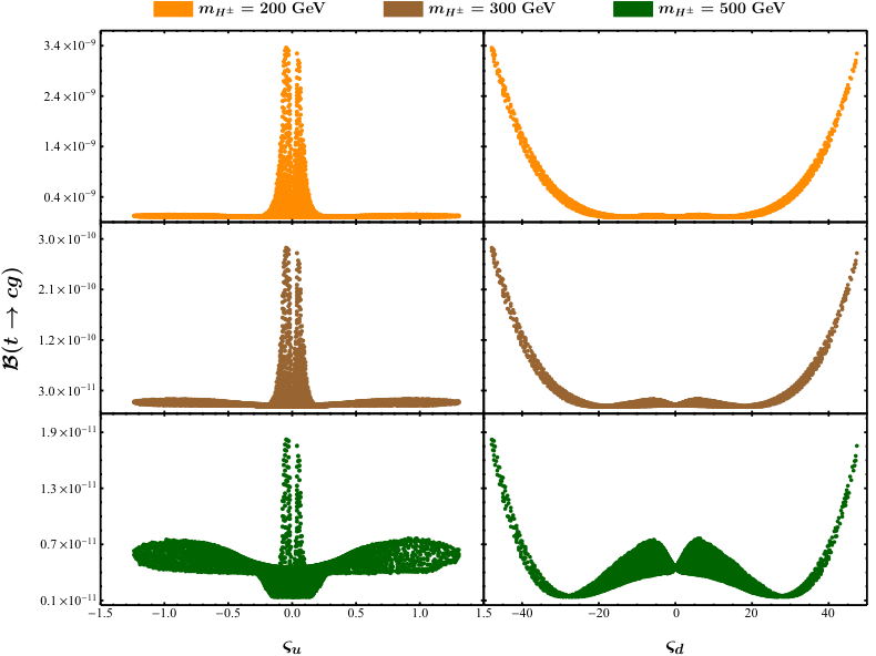
Figure 3: The branching ratio ℬ⁡(t→c​g)\mathcal{B}(t\to cg) as a function of the alignment parameters ςu\varsigma_{u} (left) and ςd\varsigma_{d} (right), for three benchmark values of the charged-Higgs mass, mH±=200m_{H^{\pm}}=200, 300300, and 500​GeV500\,{\rm GeV}, represented by the orange (top), brown (middle), and dark green (bottom) scatter plots, respectively. Here we have used the relevant constraints on the alignment parameters ςu,d\varsigma_{u,d} from a global fit obtained at the 95.5%95.5\% CL in Ref. Eberhardt:2020dat. The thickness of the shaded regions reflects the corresponding allowed range for ςd⁡(u)\varsigma_{d(u)} for a given value of ςu⁡(d)\varsigma_{u(d)}, as can be read from the brown region of the left plot of Figure 9 in Ref. Eberhardt:2020dat.
Refer to caption
Figure 4: The branching ratio ℬ⁡(t→c​g​g)\mathcal{B}(t\to cgg) as a function of the alignment parameters ςu\varsigma_{u} (left) and ςd\varsigma_{d} (right), for three benchmark values of the charged-Higgs mass, mH±=200m_{H^{\pm}}=200, 300300, and 400​GeV400\,{\rm GeV}, represented by the orange (top), brown (middle), and purple (bottom) scatter plots, respectively. The other captions are the same as in Fig. 3.

Picking up randomly the values of the alignment parameters ςu,d\varsigma_{u,d} within the brown region (corresponding to the global fit obtained at the 95.5%95.5\% CL) shown by the left plot of Figure 9 in Ref. Eberhardt:2020dat, we show in Figs. 3 and 4 the branching ratios ℬ⁡(t→c​g)\mathcal{B}(t\to cg) and ℬ⁡(t→c​g​g)\mathcal{B}(t\to cgg) as a function of ςu\varsigma_{u} (left) and ςd\varsigma_{d} (right), for three benchmark values of the charged-Higgs mass, mH±=200m_{H^{\pm}}=200, 300300, and 500​(400)​GeV500\,(400)\,{\rm GeV}, represented by the orange (top), brown (middle), and dark green (purple) (bottom) scatter plots, respectively. It can be seen that the maximum branching ratios of both t→c​gt\to cg and t→c​g​gt\to cgg decays are reached in the limits |ςu|→0|\varsigma_{u}|\to 0 and |ςd|→48|\varsigma_{d}|\to 48, which correspond to the minimum |ςu||\varsigma_{u}| and maximum |ςd||\varsigma_{d}| allowed by the combined constraints from the most constraining observables and the theoretical requirements Eberhardt:2020dat. Furthermore, almost irrespective of the values of the charged-Higgs mass, the maxima of the branching ratios are always reached with the same set of alignment parameters, (ςu,ςd)≃(−0.047,−48)(\varsigma_{u},\varsigma_{d})\simeq(-0.047,-48), when mH±m_{H^{\pm}} varies within the ranges [200,600]​GeV[200,600]\,{\rm GeV} for the t→c​gt\to cg and [200,400]​GeV[200,400]\,{\rm GeV} for the t→c​g​gt\to cgg decay. Numerically, we obtain

ℬmaxA2HDM​(t→c​g)\displaystyle\mathcal{B}^{\text{A2HDM}}_{\text{max}}(t\to cg) ={3.36×10⁻⁹,for mH±=200​GeV,2.84×10−10,for mH±=300​GeV,1.82×10−11,for mH±=500​GeV,\displaystyle=\begin{cases}3.36\times 10^{-9},&\text{for $m_{H^{\pm}}=200\,{\rm GeV}$},\\[2.84544pt] 2.84\times 10^{-10},&\text{for $m_{H^{\pm}}=300\,{\rm GeV}$},\\[2.84544pt] 1.82\times 10^{-11},&\text{for $m_{H^{\pm}}=500\,{\rm GeV}$},\end{cases} (47)

and

ℬmaxA2HDM​(t→c​g​g)\displaystyle\mathcal{B}^{\text{A2HDM}}_{\text{max}}(t\to cgg) ={2.95×10⁻⁹,for mH±=200​GeV,9.94×10−10,for mH±=300​GeV,8.60×10−10,for mH±=400​GeV.\displaystyle=\begin{cases}2.95\times 10^{-9},&\text{for $m_{H^{\pm}}=200\,{\rm GeV}$},\\[2.84544pt] 9.94\times 10^{-10},&\text{for $m_{H^{\pm}}=300\,{\rm GeV}$},\\[2.84544pt] 8.60\times 10^{-10},&\text{for $m_{H^{\pm}}=400\,{\rm GeV}$}.\end{cases} (48)

It can be seen that, with the 95.5%95.5\%-CL constraints on the alignment parameters from the global fit taken into account Eberhardt:2020dat, the maximum branching ratios of t→c​gt\to cg and t→c​g​gt\to cgg decays are both reached at mH±=200​GeVm_{H^{\pm}}=200\,{\rm GeV} and given by 3.36×10−93.36\times 10^{-9} and 2.95×10−92.95\times 10^{-9} respectively, being therefore of the same order, in the A2HDM. This is obviously different from the SM case, where the predicted branching ratio of t→c​g​gt\to cgg is about two orders of magnitude larger than that of t→c​gt\to cg (cf. Eqs. (45) and (46)) Eilam:2006uh. For convenience, we show in Fig. 5 the dependence of the maximum branching ratios of t→c​gt\to cg (left) and t→c​g​gt\to cgg (right) on the charged-Higgs mass mH±m_{H^{\pm}}, with the alignment parameters fixed at (ςu,ςd)≃(−0.047,−48)(\varsigma_{u},\varsigma_{d})\simeq(-0.047,-48).99 9 Here the plots are obtained by firstly calculating the maximum branching ratios of t→c​gt\to cg and t→c​g​gt\to cgg decays with different values of mH±m_{H^{\pm}} and the same set of alignment parameters (ςu,ςd)≃(−0.047,−48)(\varsigma_{u},\varsigma_{d})\simeq(-0.047,-48), and then constructing an interpolation of the maximum branching ratios as a function of mH±m_{H^{\pm}}. One can see that the maximum branching ratios of t→c​gt\to cg and t→c​g​gt\to cgg decays decrease sharply as the charged-Higgs mass mH±m_{H^{\pm}} increases, and approach the corresponding SM predictions for mH±≳600​GeVm_{H^{\pm}}\gtrsim 600\,{\rm GeV} and mH±≳400​GeVm_{H^{\pm}}\gtrsim 400\,{\rm GeV}, respectively.1010 10 Numerically, we find that the maximum branching ratios of t→c​gt\to cg and t→c​g​gt\to cgg decays in the A2HDM are given by 6.63×10−126.63\times 10^{-12} for mH±=600​GeVm_{H^{\pm}}=600\,{\rm GeV} and 8.60×10−108.60\times 10^{-10} for mH±=400​GeVm_{H^{\pm}}=400\,{\rm GeV} respectively, which indeed approach the corresponding SM predictions given by Eqs. (45) and (46). In addition, the maximum branching ratio ℬmaxA2HDM​(t→c​g​(g))\mathcal{B}^{\text{A2HDM}}_{\text{max}}(t\to cg(g)) will change only slightly when mH±≳600​(400)​GeVm_{H^{\pm}}\gtrsim 600~(400)\,{\rm GeV}. These observations motivate our choice of the upper limits for the charged-Higgs mass mentioned before. On the other hand, although being enhanced by about three orders of magnitude relative to the SM prediction, the maximum branching ratio of t→c​gt\to cg decay that can be reached in the A2HDM, ℬmaxA2HDM​(t→c​g)=3.36×10⁻⁹\mathcal{B}^{\text{A2HDM}}_{\text{max}}(t\to cg)=3.36\times 10^{-9}, is still at least one order of magnitude lower than the projected 95%95\%-CL limits at the future colliders, which are estimated to be 3.21×10−53.21\times 10^{-5} at the HL-LHC with 33-ab−1\text{ab}^{-1} luminosity data Cerri:2018ypt; Atlas:2019qfx, and of 𝒪⁡(10−7−10−8)\mathcal{O}(10^{-7}-10^{-8}) at the 100100-TeV\mathrm{TeV} FCC-hh with an integrated luminosity of 10​ab−110~\text{ab}^{-1} Oyulmaz:2019jqr; Khanpour:2019qnw, respectively. As a consequence, the predicted branching ratios of t→c​gt\to cg and t→c​g​gt\to cgg decays in the A2HDM are still out of the expected sensitivities of the future HL-LHC and FCC-hh.

Figure 5: The dependence of the maximum branching ratios of t→c​gt\to cg (left) and t→c​g​gt\to cgg (right) on the charged-Higgs mass mH±m_{H^{\pm}}, with the alignment parameters fixed at (ςu,ςd)≃(−0.047,−48)(\varsigma_{u},\varsigma_{d})\simeq(-0.047,-48). The horizontal dash-dotted lines represent the SM predictions given by Eqs. (45) and (46), respectively.

4.3 ℬ⁡(t→c​g​(g))\mathcal{B}(t\to cg(g)) in the conventional 2HDMs with 𝒵2\mathcal{Z}_{2} symmetries

Let us now discuss the branching ratios of t→c​gt\to cg and t→c​g​gt\to cgg decays in the four conventional 2HDMs with 𝒵2\mathcal{Z}_{2} symmetries, the Yukawa types of which have been given explicitly in Table 1. As only the charged-Higgs interactions with the quark sector are involved, we are actually left with only two different cases, type-I (type-X) 2HDM with ςd=ςu=1/tan⁡β\varsigma_{d}=\varsigma_{u}=1/\tan{\beta}, and type-II (type-Y) 2HDM with ςd=−1/ςu=−tanβ\varsigma_{d}=-1/\varsigma_{u}=-\tan{\beta}. Here, to predict the branching ratios of t→c​gt\to cg and t→c​g​gt\to cgg decays, we need only the knowledge of the charged-Higgs mass mH±m_{H^{\pm}} and the parameter tan⁡β\tan{\beta}, both of which receive severe constraints from many flavour processes and theoretical considerations Akeroyd:2016ymd; Arbey:2017gmh; Chowdhury:2017aav; Haller:2018nnx. For convenience, we show in Fig. 6 the dependence of the two branching ratios ℬ⁡(t→c​g)\mathcal{B}(t\to cg) (left) and ℬ⁡(t→c​g​g)\mathcal{B}(t\to cgg) (right) on tan⁡β\tan{\beta}, for three different choices of mH±m_{H^{\pm}}, in the four conventional 2HDMs with 𝒵2\mathcal{Z}_{2} symmetries. It should be noted that the branching ratios of t→c​gt\to cg and t→c​g​gt\to cgg decays are calculated in these four models by varying tan⁡β=[0.1,60]\tan{\beta}=[0.1,60], while the ranges where the resulting branching ratios are not significantly enhanced compared with the corresponding SM predictions are not shown in Fig. 6. It can be seen that the sensitivity of the two branching ratios to mH±m_{H^{\pm}} occurs at low and high tan⁡β\tan\beta for the type-I (type-X) and the type-II (type-Y) 2HDM respectively, and such a sensitivity becomes, however, less significant for larger mH±m_{H^{\pm}}.

Refer to caption
Refer to caption
Refer to caption
Refer to caption
Figure 6: The branching ratios of t→c​gt\to cg (left) and t→c​g​gt\to cgg (right) as a function of the parameter tan⁡β=[0.1,60]\tan{\beta}=[0.1,60], for three different choices of the charged-Higgs mass mH±m_{H^{\pm}}, in the four conventional 2HDMs with 𝒵2\mathcal{Z}_{2} symmetries. The horizontal dash-dotted lines represent the SM predictions. We show only the ranges of tan⁡β\tan{\beta} where the resulting branching ratios display significant enhancements compared with the corresponding SM predictions. Note that the charged-Higgs mass mH±m_{H^{\pm}} in type-II (type-Y) 2HDM is already bounded to be larger than 600​GeV600\,{\rm GeV} Misiak:2020vlo; Atkinson:2021eox; Hermann:2012fc, while the parameter tan⁡β\tan\beta in type-I (type-X) 2HDM is constrained to be larger than one Arbey:2017gmh, both of which imply that no significant enhancements of the branching ratios are possible in these conventional 2HDMs.

For the type-II 2HDM, the branching ratio of the weak radiative decay B¯→Xs​γ\bar{B}\to X_{s}\gamma plays a significant role in setting a lower bound on the charged-Higgs mass mH±m_{H^{\pm}}, with the latest updated results given by mH±≳800​GeVm_{H^{\pm}}\gtrsim 800\,{\rm GeV} at 95%95\% CL Misiak:2020vlo and mH±≳790​(1510)​GeVm_{H^{\pm}}\gtrsim 790\,(1510)\,{\rm GeV} at 2​σ​(1​σ)2\sigma\,(1\sigma) Atkinson:2021eox. These bounds are nearly tan⁡β\tan\beta-independent for tan⁡β>2\tan\beta>2 and show a strong dependence on tan⁡β\tan\beta only for tan⁡β<2\tan\beta<2 Hermann:2012fc. Quite recently, a comprehensive study of the allowed parameter space of the type-II 2HDM has been performed by combining the most recent flavour, collider, and electroweak precision observables with theoretical constraints, with the best fit point lying around mH±≃2​TeVm_{H^{\pm}}\simeq 2\,\mathrm{TeV} and tan⁡β≃4\tan\beta\simeq 4 Atkinson:2021eox. The experimental lower bound on mH±m_{H^{\pm}} from direct collider searches is, however, only mH±≳160​GeVm_{H^{\pm}}\gtrsim 160\,{\rm GeV} ATLAS:2018gfm, and hence well below the indirect constraints from flavour physics. With these bounds taken into account, it is then found that the branching ratios of both t→c​gt\to cg and t→c​g​gt\to cgg decays remain almost identical with the corresponding SM predictions, as given by Eqs. (45) and (46) respectively. The same conclusion can also be applied to the type-Y 2HDM, because its Yukawa type shares the same coupling pattern for the quarks as of the type-II 2HDM Arbey:2017gmh. In fact, for these two types of 2HDMs, we have ςd=−1/ςu=−tanβ\varsigma_{d}=-1/\varsigma_{u}=-\tan{\beta} and hence ςd​ςu=−1\varsigma_{d}\varsigma_{u}=-1, while the region ςd​ςu<0\varsigma_{d}\varsigma_{u}<0 is almost excluded by the current data on the branching ratio of the weak radiative decay B¯→Xs​γ\bar{B}\to X_{s}\gamma Jung:2010ik. This also implies that significant enhancements of the branching ratios of t→c​gt\to cg and t→c​g​gt\to cgg decays relative to the SM predictions are impossible in these two types of 2HDMs.

For the type-I (type-X) 2HDM, on the other hand, a 95%95\%-CL lower limit on mH±m_{H^{\pm}} from the branching ratio of B¯→Xs​γ\bar{B}\to X_{s}\gamma can be derived for low tan⁡β\tan\beta only Hermann:2012fc. As an illustration, a bound tan⁡β≲2.5\tan\beta\lesssim 2.5 can be set when the robust lower charged-Higgs mass limit mH±≳80​GeVm_{H^{\pm}}\gtrsim 80\,{\rm GeV} from the combined charged-Higgs searches at LEP ALEPH:2013htx is considered. A detailed analysis of the phenomenological status of the charged-Higgs sector in the conventional 2HDMs with 𝒵2\mathcal{Z}_{2} symmetries has been performed by combing all the constraints from direct collider searches for charged and neutral Higgs bosons, as well as the most relevant constraints from flavour physics Arbey:2017gmh. Using the combined flavour constraints at 95%95\% CL obtained there, we extract the values tan⁡β≃1.8\tan\beta\simeq 1.8 for mH±=200​GeVm_{H^{\pm}}=200\,{\rm GeV}, tan⁡β≃1.5\tan\beta\simeq 1.5 for mH±=300​GeVm_{H^{\pm}}=300\,{\rm GeV}, and tan⁡β≃1.2\tan\beta\simeq 1.2 for mH±=500​GeVm_{H^{\pm}}=500\,{\rm GeV} Arbey:2017gmh. With these typical values taken as inputs, the corresponding branching ratios of t→c​gt\to cg and t→c​g​gt\to cgg decays are given in Table 4. It can be seen that, in these two types of 2HDMs, the branching ratio of t→c​gt\to cg decay is predicted to be of the same order as in the SM (cf. Eq. (45)), while the branching ratio of t→c​g​gt\to cgg decay remains almost identical with the SM expectation (cf. Eq. (46)).

   (mH±​[GeV],tan⁡β)(m_{H^{\pm}}\,[{\rm GeV}],\,\tan\beta)       (200, 1.8)(200,\,1.8)       (300, 1.5)(300,\,1.5)       (500, 1.2)(500,\,1.2)   
   ℬType I (X)​(t→c​g)\mathcal{B}^{\text{Type I\,(X)}}(t\to cg)       5.75×10−125.75\times 10^{-12}       5.13×10−125.13\times 10^{-12}       4.85×10−124.85\times 10^{-12}   
   ℬType I (X)​(t→c​g​g)\mathcal{B}^{\text{Type I\,(X)}}(t\to cgg)       8.32×10−108.32\times 10^{-10}       8.31×10−108.31\times 10^{-10}       8.31×10−108.31\times 10^{-10}   
Table 4: The branching ratios of t→c​gt\to cg and t→c​g​gt\to cgg decays in the type-I (type-X) 2HDM, with three sets of input parameters of (mH±,tan⁡β)(m_{H^{\pm}},\tan\beta) extracted from Ref. Arbey:2017gmh.

In fact, at low tan⁡β\tan\beta, the flavour constraints are similar among all the four conventional 2HDMs with 𝒵2\mathcal{Z}_{2} symmetries, because the contributions in this case are now dominated by the universal charged-Higgs couplings to the up-type quarks (cf. Table 1). Then, it is found that values of tan⁡β<1\tan\beta<1 are ruled out for all values of mH±<650​GeVm_{H^{\pm}}<650\,{\rm GeV}, irrespective of the Yukawa types considered Arbey:2017gmh. As a summary, we can therefore conclude that, compared with the SM predictions, no significant enhancements are observed in the four conventional 2HDMs with 𝒵2\mathcal{Z}_{2} symmetries for the branching ratios of both t→c​gt\to cg and t→c​g​gt\to cgg decays, once the flavour constraints on the model parameters are taken into account.

4.4 Further discussions and comments

Let us now explain why the “higher-order dominance” phenomenon is more obvious within the SM than in the A2HDM as well as the four conventional 2HDMs with 𝒵2\mathcal{Z}_{2} symmetries. Naively, one would expect that the rate of the two-body decay t→c​gt\to cg is larger than that of the three-body decay t→c​g​gt\to cgg, due to the coupling-constant and phase-space suppression of the latter. This is, however, not true within the SM; instead, we find that the predicted branching ratio of t→c​g​gt\to cgg is about two orders of magnitude larger than that of t→c​gt\to cg (cf. Eqs. (45) and (46)) Eilam:2006uh. To understand such a “higher-order dominance” phenomenon, one should firstly note that both the t→c​gt\to cg and t→c​g​gt\to cgg decays are dominated by the one-loop effective vertex Vt​c​g∗μV_{tcg^{\ast}}^{\mu}, which can be generically written as Deshpande:1991pn

Vt​c​g∗μ=(k2γμ−kμk/)(F1LPL+F1RPR)+iσμ​νkν(F2LmcPL+F2RmtPR),\displaystyle V_{tcg^{\ast}}^{\mu}=\left(k^{2}\gamma^{\mu}-k^{\mu}k\!\!\!/\right)\left(F_{1}^{L}P_{L}+F_{1}^{R}P_{R}\right)+i\sigma^{\mu\nu}k_{\nu}\left(F_{2}^{L}m_{c}P_{L}+F_{2}^{R}m_{t}P_{R}\right)\,, (49)

as required by Lorentz and gauge invariance. Here we have suppressed both the colour labels and a sum over the internal quark flavours together with the CKM matrix elements. The form factors F1L,RF_{1}^{L,R} and F2L,RF_{2}^{L,R} are a function of the gluon virtuality k2k^{2}, and are called the monopolar (or charge radius) and the dipolar (or dipole moment) form factors, respectively. Note that when k2→0k^{2}\to 0, i.e., when the gluon goes on-shell, the F1L,RF_{1}^{L,R} contributions vanish. Therefore, the two-body decay t→c​gt\to cg is entirely determined by the dipole structure, while both the dipole and the monopole structure contribute to the three-body decay t→c​g​gt\to cgg. It also turns out that the contribution from the monopolar form factors can be considerably larger than from the dipolar ones within the SM Hou:1988wt; Simma:1990nr; Liu:1989pc; Eilam:2006uh. This explains the “higher-order dominance” phenomenon observed within the SM. For the A2HDM, however, the charged-Higgs enhancements are mostly through the dipolar form factors, and hence show up only through a greatly enhanced branching ratio of the two-body decay t→c​gt\to cg. This helps us to understand why the branching ratios of t→c​gt\to cg and t→c​g​gt\to cgg decays are predicted to be of the same order in the A2HDM. For the four conventional 2HDMs with 𝒵2\mathcal{Z}_{2} symmetries, on the other hand, after taking into account the relevant flavour constraints on the model parameters, significant enhancements are no longer allowed for the branching ratios of both t→c​gt\to cg and t→c​g​gt\to cgg decays.

Finally, we would like to make a brief comment on the observability of t→c​g​gt\to cgg decay. Note that this process can generally be treated in twofold way: One can either treat it inclusively with t→c​gt\to cg or consider it as a separate channel Eilam:2006rb. The former means that the process t→c​g​gt\to cgg can be considered as a QCD correction to the t→c​gt\to cg decay by assuring that two of the three final-state jets are collinear so that only two can be resolved by the detector. The latter is especially promising if the branching ratio of t→c​g​gt\to cgg is considerably larger than that of t→c​gt\to cg, as observed within the SM Eilam:2006uh. However, to detect t→c​g​gt\to cgg before t→c​gt\to cg, one must avoid collinearity by applying certain cuts. To this end, the cutoff parameter CC introduced in the phase space plays an essential role in distinguishing the t→c​g​gt\to cgg from the t→c​gt\to cg decay. Here, CC must be taken in the range of jet-energy resolution of the detector, and a better jet resolution will be definitely welcome.

5 Conclusion

In this paper, we have firstly updated the SM predictions for the branching ratios of both t→c​gt\to cg and t→c​g​gt\to cgg decays, with the results given respectively by ℬSM​(t→c​g)=4.50×10⁻¹²\mathcal{B}^{\text{SM}}(t\to cg)=4.50\times 10^{-12} and ℬSM​(t→c​g​g)=8.31×10⁻¹⁰\mathcal{B}^{\text{SM}}(t\to cgg)=8.31\times 10^{-10}, finding that the latter is about two orders of magnitude larger than the former, which is a clear demonstration of the “higher-order dominance” phenomenon observed in Ref. Eilam:2006uh. This is due to the fact that the contribution from the monopolar form factors can be considerably larger than from the dipolar ones within the SM Hou:1988wt; Simma:1990nr; Liu:1989pc; Eilam:2006uh. Note that the branching ratio of the three-body decay t→c​g​gt\to cgg is obtained with the cutoff parameter C=0.01C=0.01.

To check if such a “higher-order dominance” phenomenon is also applied in the A2HDM as well as in the four conventional 2HDMs with 𝒵2\mathcal{Z}_{2} symmetries, we have also evaluated the maximum branching ratios of t→c​gt\to cg and t→c​g​gt\to cgg decays that can be reached in these different models. After taking into account the relevant constraints on the model parameters resulting from a global fit obtained at the 95.5%95.5\% CL Eberhardt:2020dat, we find that the branching ratios of t→c​gt\to cg and t→c​g​gt\to cgg decays can reach up to 3.36×10−93.36\times 10^{-9} and 2.95×10−92.95\times 10^{-9} respectively, being therefore of the same order, in the A2HDM. This is obviously different from the SM case, and can be understood by the fact that the charged-Higgs enhancements are mostly through the dipolar form factors, and hence show up only through a greatly enhanced branching ratio of the two-body decay t→c​gt\to cg. On the other hand, compared with the SM predictions, significant enhancements are no longer possible in the four conventional 2HDMs with 𝒵2\mathcal{Z}_{2} symmetries for the branching ratios of these two decays, once the flavour constraints on the model parameters Atkinson:2021eox; Arbey:2017gmh are properly taken into account.

Nevertheless, the predicted branching ratios of t→c​gt\to cg and t→c​g​gt\to cgg decays in the A2HDM are still out of the expected sensitivities of the future HL-LHC and FCC-hh. To have an opportunity to detect t→c​g​gt\to cgg before t→c​gt\to cg, we have to improve the jet resolution of the future detector. Note that, due to the imaginary components of the loop functions, the CKM matrix elements, as well as the complex alignment parameters ςu,d\varsigma_{u,d} in the A2HDM, it would also be interesting to investigate the CP asymmetries in these rare top-quark decays Balaji:2020qjg; AguilarSaavedra:2002ns.

Acknowledgements

We are very grateful to Thomas Hahn for useful communications on the function PolarizationSum defined in the package FormCalc. This work is supported by the National Natural Science Foundation of China under Grant Nos. 12135006, 12075097, 11947213, 11675061 and 11775092, as well as by the Fundamental Research Funds for the Central Universities under Grant Nos. CCNU20TS007, CCNU19TD012 and CCNU22LJ004. S.F. is also supported by the International Postdoctoral Exchange Fellowship Program.

Appendix A The 𝑹R functions relevant for 𝒕→𝒄​𝒈​𝒈t\to cgg decay

In this appendix, we give the explicit expressions of the remaining RR functions present in Eqs. (32)–(34). For convenience, the scalar products involved are defined in the same way as in Ref. Eilam:2006uh, with

SP1 =ϵ∗​(k3)⋅ϵ∗​(k4),\displaystyle=\epsilon^{*}(k_{3})\cdot\epsilon^{*}(k_{4}), SP2=ϵ∗​(k3)⋅k1,\displaystyle\text{SP2}=\epsilon^{*}(k_{3})\cdot k_{1}, SP3=ϵ∗​(k3)⋅k2,\displaystyle\text{SP3}=\epsilon^{*}(k_{3})\cdot k_{2},
SP4 =ϵ∗​(k4)⋅k1,\displaystyle=\epsilon^{*}(k_{4})\cdot k_{1}, SP5=ϵ∗​(k4)⋅k2.\displaystyle\text{SP5}=\epsilon^{*}(k_{4})\cdot k_{2}. (50)

For the vertex part (cf. Eqs. (32)), we have

R1vertex\displaystyle R_{1}^{\text{vertex}} =\displaystyle= −(SP1​F5−F16)​(mW2​(1−2​(B0(3)​(mW2)−2​C00(3)​(mW2)−s23​C2(3)​(mW2)))CLOSE\displaystyle-(\text{SP1}\,F_{5}-F_{16})(m_{W}^{2}(1-2(B_{0}^{(3)}(m_{W}^{2})-2C_{00}^{(3)}(m_{W}^{2})-s_{23}C_{2}^{(3)}(m_{W}^{2}))) (51)
−\displaystyle- mb2​(mt2​(C0(3)​(mW2)+C2(3)​(mW2)+Xd​d​C2(3)​(mH±2)+Xd​u​C0(3)​(mH±2))+B0(3)​(mW2)CLOSE\displaystyle m_{b}^{2}(m_{t}^{2}(C_{0}^{(3)}(m_{W}^{2})+C_{2}^{(3)}(m_{W}^{2})+\text{X}_{dd}C_{2}^{(3)}(m_{H^{\pm}}^{2})+\text{X}_{du}C_{0}^{(3)}(m_{H^{\pm}}^{2}))+B_{0}^{(3)}(m_{W}^{2})
+\displaystyle+ OPENOPENXd​d​B0(3)​(mH±2)−2​(C00(3)​(mW2)+Xd​d​C00(3)​(mH±2))))+mt​(s23​(SP1​F1−F12)CLOSE\displaystyle\text{X}_{dd}B_{0}^{(3)}(m_{H^{\pm}}^{2})-2(C_{00}^{(3)}(m_{W}^{2})+\text{X}_{dd}C_{00}^{(3)}(m_{H^{\pm}}^{2}))))+m_{t}(s_{23}(\text{SP1}\,F_{1}-F_{12})
(2​mW2​C2(3)​(mW2)−mb2​(C0(3)​(mW2)+C2(3)​(mW2)+Xd​d​C2(3)​(mH±2)CLOSECLOSE\displaystyle(2m_{W}^{2}C_{2}^{(3)}(m_{W}^{2})-m_{b}^{2}(C_{0}^{(3)}(m_{W}^{2})+C_{2}^{(3)}(m_{W}^{2})+\text{X}_{dd}C_{2}^{(3)}(m_{H^{\pm}}^{2})
+\displaystyle+ OPENOPENXd​u​C0(3)​(mH±2)))+2​SP4​(2​SP3​F1−F13)​(mb2​(C0(3)​(mW2)+2​C2(3)​(mW2)CLOSECLOSE\displaystyle\text{X}_{du}C_{0}^{(3)}(m_{H^{\pm}}^{2})))+2\text{SP4}(2\text{SP3}\,F_{1}-F_{13})(m_{b}^{2}(C_{0}^{(3)}(m_{W}^{2})+2C_{2}^{(3)}(m_{W}^{2})
+\displaystyle+ C22(3)​(mW2)+Xd​d​(C12(3)​(mH±2)+C2(3)​(mH±2)+C22(3)​(mH±2))+Xd​u​(C0(3)​(mH±2)CLOSE\displaystyle C_{22}^{(3)}(m_{W}^{2})+\text{X}_{dd}(C_{12}^{(3)}(m_{H^{\pm}}^{2})+C_{2}^{(3)}(m_{H^{\pm}}^{2})+C_{22}^{(3)}(m_{H^{\pm}}^{2}))+\text{X}_{du}(C_{0}^{(3)}(m_{H^{\pm}}^{2})
+\displaystyle+ C2(3)(mH±2)))+2mW2C22(3)(mW2)+(mb2+2mW2)C12(3)(mW2)))\displaystyle C_{2}^{(3)}(m_{H^{\pm}}^{2})))+2m_{W}^{2}C_{22}^{(3)}(m_{W}^{2})+(m_{b}^{2}+2m_{W}^{2})C_{12}^{(3)}(m_{W}^{2})))
+\displaystyle+ F3​(−(mt2​(SP4​C2(3)​(mW2)−SP5​Xd​d​C2(3)​(mH±2))+SP4​(B0(3)​(mW2)−2​C00(3)​(mW2))CLOSECLOSE\displaystyle F_{3}(-(m_{t}^{2}(\text{SP4}C_{2}^{(3)}(m_{W}^{2})-\text{SP5}\,\text{X}_{dd}C_{2}^{(3)}(m_{H^{\pm}}^{2}))+\text{SP4}(B_{0}^{(3)}(m_{W}^{2})-2C_{00}^{(3)}(m_{W}^{2}))
+\displaystyle+ (SP4−SP5)​(mt2​(C0(3)​(mW2)+Xd​u​C0(3)​(mH±2))+(B0(3)​(mH±2)CLOSECLOSE\displaystyle(\text{SP4}-\text{SP5})(m_{t}^{2}(C_{0}^{(3)}(m_{W}^{2})+\text{X}_{du}C_{0}^{(3)}(m_{H^{\pm}}^{2}))+(B_{0}^{(3)}(m_{H^{\pm}}^{2})
−\displaystyle- 2C00(3)(mH±2))Xd​d))mb2+(SP4−SP5)mW2+(B0(3)(mW2)−2C00(3)(mW2))(SP5mb2\displaystyle 2C_{00}^{(3)}(m_{H^{\pm}}^{2}))\text{X}_{dd}))m_{b}^{2}+(\text{SP4}-\text{SP5})m_{W}^{2}+(B_{0}^{(3)}(m_{W}^{2})-2C_{00}^{(3)}(m_{W}^{2}))(\text{SP5}m_{b}^{2}
−\displaystyle- OPEN2​(SP4−SP5)​mW2)+C2(3)​(mW2)​(SP5​mb2​mt2−2​s23​(SP4+SP5)​mW2)\displaystyle 2(\text{SP4}-\text{SP5})m_{W}^{2})+C_{2}^{(3)}(m_{W}^{2})(\text{SP5}m_{b}^{2}m_{t}^{2}-2s_{23}(\text{SP4}+\text{SP5})m_{W}^{2})
−\displaystyle- OPENSP4​((2​s23​C12(3)​(mH±2)+mt2​C2(3)​(mH±2))​Xd​d​mb2+2​s23​C12(3)​(mW2)​(mb2+2​mW2)))\displaystyle\text{SP4}((2s_{23}C_{12}^{(3)}(m_{H^{\pm}}^{2})+m_{t}^{2}C_{2}^{(3)}(m_{H^{\pm}}^{2}))\text{X}_{dd}m_{b}^{2}+2s_{23}C_{12}^{(3)}(m_{W}^{2})(m_{b}^{2}+2m_{W}^{2})))
+\displaystyle+ SP3F4((4(C00(3)(mW2)+C00(3)(mH±2)Xd​d)−2((C0(3)(mW2)+C2(3)(mW2)\displaystyle\text{SP3}\,F_{4}((4(C_{00}^{(3)}(m_{W}^{2})+C_{00}^{(3)}(m_{H^{\pm}}^{2})\text{X}_{dd})-2((C_{0}^{(3)}(m_{W}^{2})+C_{2}^{(3)}(m_{W}^{2})
+\displaystyle+ C2(3)(mH±2)Xd​d+C0(3)(mH±2)Xd​u)mt2+B0(3)(mW2)+B0(3)(mH±2)Xd​d))mb2\displaystyle C_{2}^{(3)}(m_{H^{\pm}}^{2})\text{X}_{dd}+C_{0}^{(3)}(m_{H^{\pm}}^{2})\text{X}_{du})m_{t}^{2}+B_{0}^{(3)}(m_{W}^{2})+B_{0}^{(3)}(m_{H^{\pm}}^{2})\text{X}_{dd}))m_{b}^{2}
+\displaystyle+ OPEN(−4​B0(3)​(mW2)+8​C00(3)​(mW2)+4​s23​C2(3)​(mW2)+2)​mW2),\displaystyle(-4B_{0}^{(3)}(m_{W}^{2})+8C_{00}^{(3)}(m_{W}^{2})+4s_{23}C_{2}^{(3)}(m_{W}^{2})+2)m_{W}^{2}),
R2vertex\displaystyle R_{2}^{\text{vertex}} =\displaystyle= (2(s23(SP4−SP5)C2(2)(mW2)F3+SP3F4)mW2−(SP1F5−F16)((−2B0(3)(mW2)\displaystyle(2(s_{23}(\text{SP4}-\text{SP5})C_{2}^{(2)}(m_{W}^{2})F_{3}+\text{SP3}\,F_{4})m_{W}^{2}-(\text{SP1}\,F_{5}-F_{16})((-2B_{0}^{(3)}(m_{W}^{2}) (52)
+\displaystyle+ OPEN4​C00(2)​(mW2)+2​s23​C2(2)​(mW2)+1)​mW2−mb2​((C0(2)​(mW2)+C0(2)​(mH±2)​Xd​u)​mt2CLOSE\displaystyle 4C_{00}^{(2)}(m_{W}^{2})+2s_{23}C_{2}^{(2)}(m_{W}^{2})+1)m_{W}^{2}-m_{b}^{2}((C_{0}^{(2)}(m_{W}^{2})+C_{0}^{(2)}(m_{H^{\pm}}^{2})\text{X}_{du})m_{t}^{2}
+\displaystyle+ OPENOPENB0(3)​(mW2)+B0(3)​(mH±2)​Xd​d−2​(C00(2)​(mW2)+C00(2)​(mH±2)​Xd​d)))+(SP4−SP5)​F3\displaystyle B_{0}^{(3)}(m_{W}^{2})+B_{0}^{(3)}(m_{H^{\pm}}^{2})\text{X}_{dd}-2(C_{00}^{(2)}(m_{W}^{2})+C_{00}^{(2)}(m_{H^{\pm}}^{2})\text{X}_{dd})))+(\text{SP4}-\text{SP5})F_{3}
(−B0(3)(mH±2)Xd​dmb2+(2(C00(2)(mW2)+C00(2)(mH±2)Xd​d)−mt2(C0(2)(mW2)\displaystyle(-B_{0}^{(3)}(m_{H^{\pm}}^{2})\text{X}_{dd}m_{b}^{2}+(2(C_{00}^{(2)}(m_{W}^{2})+C_{00}^{(2)}(m_{H^{\pm}}^{2})\text{X}_{dd})-m_{t}^{2}(C_{0}^{(2)}(m_{W}^{2})
+\displaystyle+ C0(2)(mH±2)Xd​u))mb2+(4C00(2)(mW2)+1)mW2−B0(3)(mW2)(mb2+2mW2))\displaystyle C_{0}^{(2)}(m_{H^{\pm}}^{2})\text{X}_{du}))m_{b}^{2}+(4C_{00}^{(2)}(m_{W}^{2})+1)m_{W}^{2}-B_{0}^{(3)}(m_{W}^{2})(m_{b}^{2}+2m_{W}^{2}))
−\displaystyle- SP3F4(4(B0(3)(mW2)−2C00(2)(mW2))mW2+2((−(C2(2)(mW2)+C2(2)(mH±2)Xd​u)mt2\displaystyle\text{SP3}\,F_{4}(4(B_{0}^{(3)}(m_{W}^{2})-2C_{00}^{(2)}(m_{W}^{2}))m_{W}^{2}+2((-(C_{2}^{(2)}(m_{W}^{2})+C_{2}^{(2)}(m_{H^{\pm}}^{2})\text{X}_{du})m_{t}^{2}
+\displaystyle+ OPENB0(3)​(mW2)+B0(3)​(mH±2)​Xd​d−2​(C00(2)​(mW2)+C00(2)​(mH±2)​Xd​d))​mb2\displaystyle B_{0}^{(3)}(m_{W}^{2})+B_{0}^{(3)}(m_{H^{\pm}}^{2})\text{X}_{dd}-2(C_{00}^{(2)}(m_{W}^{2})+C_{00}^{(2)}(m_{H^{\pm}}^{2})\text{X}_{dd}))m_{b}^{2}
+\displaystyle+ s23(C12(2)(mH±2)Xd​dmb2+C12(2)(mW2)(mb2+2mW2))))+mt(−F12((1−2(B0(3)(mW2)\displaystyle s_{23}(C_{12}^{(2)}(m_{H^{\pm}}^{2})\text{X}_{dd}m_{b}^{2}+C_{12}^{(2)}(m_{W}^{2})(m_{b}^{2}+2m_{W}^{2}))))+m_{t}(-F_{12}((1-2(B_{0}^{(3)}(m_{W}^{2})
−\displaystyle- OPENOPEN2​C00(2)​(mW2)−s23​C2(2)​(mW2)))​mW2−mb2​(B0(3)​(mW2)+B0(3)​(mH±2)​Xd​dCLOSE\displaystyle 2C_{00}^{(2)}(m_{W}^{2})-s_{23}C_{2}^{(2)}(m_{W}^{2})))m_{W}^{2}-m_{b}^{2}(B_{0}^{(3)}(m_{W}^{2})+B_{0}^{(3)}(m_{H^{\pm}}^{2})\text{X}_{dd}
−\displaystyle- OPENOPEN2​(C00(2)​(mW2)+C00(2)​(mH±2)​Xd​d)+s23​(C0(2)​(mW2)+C0(2)​(mH±2)​Xd​u)))\displaystyle 2(C_{00}^{(2)}(m_{W}^{2})+C_{00}^{(2)}(m_{H^{\pm}}^{2})\text{X}_{dd})+s_{23}(C_{0}^{(2)}(m_{W}^{2})+C_{0}^{(2)}(m_{H^{\pm}}^{2})\text{X}_{du})))
−\displaystyle- SP3F14((2(C12(2)(mW2)+C12(2)(mH±2)Xd​d)−2(C0(2)(mW2)+C2(2)(mW2)\displaystyle\text{SP3}\,F_{14}((2(C_{12}^{(2)}(m_{W}^{2})+C_{12}^{(2)}(m_{H^{\pm}}^{2})\text{X}_{dd})-2(C_{0}^{(2)}(m_{W}^{2})+C_{2}^{(2)}(m_{W}^{2})
+\displaystyle+ (C0(2)(mH±2)+C2(2)(mH±2))Xd​u))mb2+4(C12(2)(mW2)+C2(2)(mW2))mW2)\displaystyle(C_{0}^{(2)}(m_{H^{\pm}}^{2})+C_{2}^{(2)}(m_{H^{\pm}}^{2}))\text{X}_{du}))m_{b}^{2}+4(C_{12}^{(2)}(m_{W}^{2})+C_{2}^{(2)}(m_{W}^{2}))m_{W}^{2})
+\displaystyle+ F1(−((s23SP1−2SP3(SP4−SP5))C0(2)(mW2)−2(SP1(C00(2)(mW2)\displaystyle F_{1}(-((s_{23}\text{SP1}-2\text{SP3}(\text{SP4}-\text{SP5}))C_{0}^{(2)}(m_{W}^{2})-2(\text{SP1}(C_{00}^{(2)}(m_{W}^{2})
+\displaystyle+ C00(2)(mH±2)Xd​d)+SP3(SP4−SP5)C0(2)(mH±2)Xd​u))mb2+2C2(2)(mW2)(s23SP1mW2\displaystyle C_{00}^{(2)}(m_{H^{\pm}}^{2})\text{X}_{dd})+\text{SP3}(\text{SP4}-\text{SP5})C_{0}^{(2)}(m_{H^{\pm}}^{2})\text{X}_{du}))m_{b}^{2}+2C_{2}^{(2)}(m_{W}^{2})(s_{23}\text{SP1}m_{W}^{2}
+\displaystyle+ OPENSP3​(SP4−SP5)​(mb2−2​mW2))+SP1​(−(B0(3)​(mH±2)​Xd​d+s23​C0(2)​(mH±2)​Xd​u)​mb2CLOSE\displaystyle\text{SP3}(\text{SP4}-\text{SP5})(m_{b}^{2}-2m_{W}^{2}))+\text{SP1}(-(B_{0}^{(3)}(m_{H^{\pm}}^{2})\text{X}_{dd}+s_{23}C_{0}^{(2)}(m_{H^{\pm}}^{2})\text{X}_{du})m_{b}^{2}
+\displaystyle+ OPEN(4​C00(2)​(mW2)+1)​mW2−B0(3)​(mW2)​(mb2+2​mW2))−2​SP3​(SP4−SP5)\displaystyle(4C_{00}^{(2)}(m_{W}^{2})+1)m_{W}^{2}-B_{0}^{(3)}(m_{W}^{2})(m_{b}^{2}+2m_{W}^{2}))-2\text{SP3}(\text{SP4}-\text{SP5})
OPENOPEN((C12(2)​(mH±2)​Xd​d−C2(2)​(mH±2)​Xd​u)​mb2+C12(2)​(mW2)​(mb2+2​mW2)))),\displaystyle((C_{12}^{(2)}(m_{H^{\pm}}^{2})\text{X}_{dd}-C_{2}^{(2)}(m_{H^{\pm}}^{2})\text{X}_{du})m_{b}^{2}+C_{12}^{(2)}(m_{W}^{2})(m_{b}^{2}+2m_{W}^{2})))),
R3vertex\displaystyle R_{3}^{\text{vertex}} =\displaystyle= −((2(SP4−SP5)tC2(5)(mW2)F3−2SP2F4)mW2−SP1F5((−2B0(4)(mW2)\displaystyle-((2(\text{SP4}-\text{SP5})tC_{2}^{(5)}(m_{W}^{2})F_{3}-2\text{SP2}\,F_{4})m_{W}^{2}-\text{SP1}\,F_{5}((-2B_{0}^{(4)}(m_{W}^{2}) (53)
+\displaystyle+ OPEN4​C00(5)​(mW2)+2​t​C2(5)​(mW2)+1)​mW2−mb2​(mt2​(C0(5)​(mW2)+C2(5)​(mW2)CLOSECLOSE\displaystyle 4C_{00}^{(5)}(m_{W}^{2})+2tC_{2}^{(5)}(m_{W}^{2})+1)m_{W}^{2}-m_{b}^{2}(m_{t}^{2}(C_{0}^{(5)}(m_{W}^{2})+C_{2}^{(5)}(m_{W}^{2})
+\displaystyle+ OPENC2(5)​(mH±2)​Xd​d+C0(5)​(mH±2)​Xd​u)+B0(4)​(mW2)+B0(4)​(mH±2)​Xd​d−2​(C00(5)​(mW2)CLOSE\displaystyle C_{2}^{(5)}(m_{H^{\pm}}^{2})\text{X}_{dd}+C_{0}^{(5)}(m_{H^{\pm}}^{2})\text{X}_{du})+B_{0}^{(4)}(m_{W}^{2})+B_{0}^{(4)}(m_{H^{\pm}}^{2})\text{X}_{dd}-2(C_{00}^{(5)}(m_{W}^{2})
+\displaystyle+ C00(5)(mH±2)Xd​d)))−F16((1−2(B0(4)(mW2)−2C00(5)(mW2)−tC2(5)(mW2)))mW2\displaystyle C_{00}^{(5)}(m_{H^{\pm}}^{2})\text{X}_{dd})))-F_{16}((1-2(B_{0}^{(4)}(m_{W}^{2})-2C_{00}^{(5)}(m_{W}^{2})-tC_{2}^{(5)}(m_{W}^{2})))m_{W}^{2}
−\displaystyle- mb2​(mt2​(C0(5)​(mW2)+C2(5)​(mW2)+C2(5)​(mH±2)​Xd​d+C0(5)​(mH±2)​Xd​u)+B0(4)​(mW2)CLOSE\displaystyle m_{b}^{2}(m_{t}^{2}(C_{0}^{(5)}(m_{W}^{2})+C_{2}^{(5)}(m_{W}^{2})+C_{2}^{(5)}(m_{H^{\pm}}^{2})\text{X}_{dd}+C_{0}^{(5)}(m_{H^{\pm}}^{2})\text{X}_{du})+B_{0}^{(4)}(m_{W}^{2})
+\displaystyle+ OPENOPENB0(4)​(mH±2)​Xd​d−2​(C00(5)​(mW2)+C00(5)​(mH±2)​Xd​d)))\displaystyle B_{0}^{(4)}(m_{H^{\pm}}^{2})\text{X}_{dd}-2(C_{00}^{(5)}(m_{W}^{2})+C_{00}^{(5)}(m_{H^{\pm}}^{2})\text{X}_{dd})))
+\displaystyle+ (SP4−SP5)​F3​(−B0(4)​(mH±2)​Xd​d​mb2+mb2​(2​(C00(5)​(mW2)+C00(5)​(mH±2)​Xd​d)CLOSECLOSE\displaystyle(\text{SP4}-\text{SP5})F_{3}(-B_{0}^{(4)}(m_{H^{\pm}}^{2})\text{X}_{dd}m_{b}^{2}+m_{b}^{2}(2(C_{00}^{(5)}(m_{W}^{2})+C_{00}^{(5)}(m_{H^{\pm}}^{2})\text{X}_{dd})
−\displaystyle- OPENmt2​(C0(5)​(mW2)+C2(5)​(mW2)+C2(5)​(mH±2)​Xd​d+C0(5)​(mH±2)​Xd​u))\displaystyle m_{t}^{2}(C_{0}^{(5)}(m_{W}^{2})+C_{2}^{(5)}(m_{W}^{2})+C_{2}^{(5)}(m_{H^{\pm}}^{2})\text{X}_{dd}+C_{0}^{(5)}(m_{H^{\pm}}^{2})\text{X}_{du}))
+\displaystyle+ (4C00(5)(mW2)+1)mW2−B0(4)(mW2)(mb2+2mW2))+SP2F4(−(2mb2(C2(5)(mW2)\displaystyle(4C_{00}^{(5)}(m_{W}^{2})+1)m_{W}^{2}-B_{0}^{(4)}(m_{W}^{2})(m_{b}^{2}+2m_{W}^{2}))+\text{SP2}\,F_{4}(-(2m_{b}^{2}(C_{2}^{(5)}(m_{W}^{2})
+\displaystyle+ OPENOPENC22(5)​(mW2)+C22(5)​(mH±2)​Xd​d+C2(5)​(mH±2)​Xd​u)+4​C22(5)​(mW2)​mW2)​mt2\displaystyle C_{22}^{(5)}(m_{W}^{2})+C_{22}^{(5)}(m_{H^{\pm}}^{2})\text{X}_{dd}+C_{2}^{(5)}(m_{H^{\pm}}^{2})\text{X}_{du})+4C_{22}^{(5)}(m_{W}^{2})m_{W}^{2})m_{t}^{2}
+\displaystyle+ 4mW2(B0(4)(mW2)−2C00(5)(mW2))+2((−C12(5)(mW2)mt2+B0(4)(mW2)+(B0(4)(mH±2)\displaystyle 4m_{W}^{2}(B_{0}^{(4)}(m_{W}^{2})-2C_{00}^{(5)}(m_{W}^{2}))+2((-C_{12}^{(5)}(m_{W}^{2})m_{t}^{2}+B_{0}^{(4)}(m_{W}^{2})+(B_{0}^{(4)}(m_{H^{\pm}}^{2})
−\displaystyle- OPENOPEN(s23+t12)​C12(5)​(mH±2))​Xd​d−2​(C00(5)​(mW2)+C00(5)​(mH±2)​Xd​d))​mb2+C12(5)​(mW2)​(t​mb2CLOSE\displaystyle(s_{23}+t_{12})C_{12}^{(5)}(m_{H^{\pm}}^{2}))\text{X}_{dd}-2(C_{00}^{(5)}(m_{W}^{2})+C_{00}^{(5)}(m_{H^{\pm}}^{2})\text{X}_{dd}))m_{b}^{2}+C_{12}^{(5)}(m_{W}^{2})(tm_{b}^{2}
−\displaystyle- 2(s23+t12)mW2)))+mt(−SP2F14(2mb2(C0(5)(mW2)+C12(5)(mW2)+C22(5)(mW2)\displaystyle 2(s_{23}+t_{12})m_{W}^{2})))+m_{t}(-\text{SP2}\,F_{14}(2m_{b}^{2}(C_{0}^{(5)}(m_{W}^{2})+C_{12}^{(5)}(m_{W}^{2})+C_{22}^{(5)}(m_{W}^{2})
+\displaystyle+ OPEN(C12(5)​(mH±2)+C22(5)​(mH±2))​Xd​d+C0(5)​(mH±2)​Xd​u+C2(5)​(mH±2)​(Xd​d+Xd​u))\displaystyle(C_{12}^{(5)}(m_{H^{\pm}}^{2})+C_{22}^{(5)}(m_{H^{\pm}}^{2}))\text{X}_{dd}+C_{0}^{(5)}(m_{H^{\pm}}^{2})\text{X}_{du}+C_{2}^{(5)}(m_{H^{\pm}}^{2})(\text{X}_{dd}+\text{X}_{du}))
+\displaystyle+ OPEN4​(C2(5)​(mW2)​mb2+(C12(5)​(mW2)+C22(5)​(mW2))​mW2))+F12​(mW2​(−2​B0(4)​(mW2)CLOSECLOSE\displaystyle 4(C_{2}^{(5)}(m_{W}^{2})m_{b}^{2}+(C_{12}^{(5)}(m_{W}^{2})+C_{22}^{(5)}(m_{W}^{2}))m_{W}^{2}))+F_{12}(m_{W}^{2}(-2B_{0}^{(4)}(m_{W}^{2})
+\displaystyle+ OPEN4​C00(5)​(mW2)+1)−mb2​(B0(4)​(mW2)+B0(4)​(mH±2)​Xd​d−2​(C00(5)​(mW2)CLOSECLOSE\displaystyle 4C_{00}^{(5)}(m_{W}^{2})+1)-m_{b}^{2}(B_{0}^{(4)}(m_{W}^{2})+B_{0}^{(4)}(m_{H^{\pm}}^{2})\text{X}_{dd}-2(C_{00}^{(5)}(m_{W}^{2})
+\displaystyle+ OPENC00(5)​(mH±2)​Xd​d)+(s23+t12)​(C0(5)​(mW2)+C2(5)​(mW2)+C2(5)​(mH±2)​Xd​dCLOSE\displaystyle C_{00}^{(5)}(m_{H^{\pm}}^{2})\text{X}_{dd})+(s_{23}+t_{12})(C_{0}^{(5)}(m_{W}^{2})+C_{2}^{(5)}(m_{W}^{2})+C_{2}^{(5)}(m_{H^{\pm}}^{2})\text{X}_{dd}
+\displaystyle+ C0(5)(mH±2)Xd​u)))−F1(mb2((s23SP1+t12SP1+SP2(2SP5−2SP4))C0(5)(mW2)\displaystyle C_{0}^{(5)}(m_{H^{\pm}}^{2})\text{X}_{du})))-F_{1}(m_{b}^{2}((s_{23}\text{SP1}+t_{12}\text{SP1}+\text{SP2}(2\text{SP5}-2\text{SP4}))C_{0}^{(5)}(m_{W}^{2})
−\displaystyle- (4​SP2​(SP4−SP5)+SP1​t)​C2(5)​(mW2)−SP1​(−C2(5)​(mW2)​mt2+2​C00(5)​(mW2)CLOSE\displaystyle(4\text{SP2}(\text{SP4}-\text{SP5})+\text{SP1}t)C_{2}^{(5)}(m_{W}^{2})-\text{SP1}(-C_{2}^{(5)}(m_{W}^{2})m_{t}^{2}+2C_{00}^{(5)}(m_{W}^{2})
+\displaystyle+ OPEN(2​C00(5)​(mH±2)+t​C2(5)​(mH±2))​Xd​d)−2​SP2​(SP4​C22(5)​(mW2)CLOSE\displaystyle(2C_{00}^{(5)}(m_{H^{\pm}}^{2})+tC_{2}^{(5)}(m_{H^{\pm}}^{2}))\text{X}_{dd})-2\text{SP2}(\text{SP4}C_{22}^{(5)}(m_{W}^{2})
+\displaystyle+ OPEN(SP4−SP5)​C22(5)​(mH±2)​Xd​d)−(2​SP2​(SP4−SP5)+SP1​t)​C0(5)​(mH±2)​Xd​u\displaystyle(\text{SP4}-\text{SP5})C_{22}^{(5)}(m_{H^{\pm}}^{2})\text{X}_{dd})-(2\text{SP2}(\text{SP4}-\text{SP5})+\text{SP1}t)C_{0}^{(5)}(m_{H^{\pm}}^{2})\text{X}_{du}
+\displaystyle+ OPENC2(5)​(mH±2)​(SP1​mt2​Xd​d−2​SP2​(SP4−SP5)​(Xd​d+Xd​u)))+2​SP2​((C12(5)​(mW2)CLOSECLOSE\displaystyle C_{2}^{(5)}(m_{H^{\pm}}^{2})(\text{SP1}m_{t}^{2}\text{X}_{dd}-2\text{SP2}(\text{SP4}-\text{SP5})(\text{X}_{dd}+\text{X}_{du})))+2\text{SP2}((C_{12}^{(5)}(m_{W}^{2})
+\displaystyle+ OPENC22(5)​(mW2))​(SP5​mb2−2​(SP4−SP5)​mW2)−mb2​(SP4​C12(5)​(mW2)CLOSE\displaystyle C_{22}^{(5)}(m_{W}^{2}))(\text{SP5}m_{b}^{2}-2(\text{SP4}-\text{SP5})m_{W}^{2})-m_{b}^{2}(\text{SP4}C_{12}^{(5)}(m_{W}^{2})
+\displaystyle+ OPENOPEN(SP4−SP5)​C12(5)​(mH±2)​Xd​d))−SP1​(−mb2​(C0(5)​(mH±2)​Xd​u​mt2+B0(4)​(mH±2)​Xd​d)CLOSE\displaystyle(\text{SP4}-\text{SP5})C_{12}^{(5)}(m_{H^{\pm}}^{2})\text{X}_{dd}))-\text{SP1}(-m_{b}^{2}(C_{0}^{(5)}(m_{H^{\pm}}^{2})\text{X}_{du}m_{t}^{2}+B_{0}^{(4)}(m_{H^{\pm}}^{2})\text{X}_{dd})
+\displaystyle+ (4C00(5)(mW2)+1)mW2−B0(4)(mW2)(mb2+2mW2))))),\displaystyle(4C_{00}^{(5)}(m_{W}^{2})+1)m_{W}^{2}-B_{0}^{(4)}(m_{W}^{2})(m_{b}^{2}+2m_{W}^{2}))))),
R4vertex\displaystyle R_{4}^{\text{vertex}} =\displaystyle= F16((−2B0(4)(mW2)+4C00(4)(mW2)+2tC2(4)(mW2)+1)mW2−mb2((C0(4)(mW2)\displaystyle F_{16}((-2B_{0}^{(4)}(m_{W}^{2})+4C_{00}^{(4)}(m_{W}^{2})+2tC_{2}^{(4)}(m_{W}^{2})+1)m_{W}^{2}-m_{b}^{2}((C_{0}^{(4)}(m_{W}^{2}) (54)
+\displaystyle+ OPENC0(4)​(mH±2)​Xd​u)​mt2+B0(4)​(mW2)+B0(4)​(mH±2)​Xd​d−2​(C00(4)​(mW2)CLOSE\displaystyle C_{0}^{(4)}(m_{H^{\pm}}^{2})\text{X}_{du})m_{t}^{2}+B_{0}^{(4)}(m_{W}^{2})+B_{0}^{(4)}(m_{H^{\pm}}^{2})\text{X}_{dd}-2(C_{00}^{(4)}(m_{W}^{2})
+\displaystyle+ C00(4)(mH±2)Xd​d)))+SP1F5(mW2(1−2(B0(4)(mW2)−2C00(4)(mW2)−tC2(4)(mW2)))\displaystyle C_{00}^{(4)}(m_{H^{\pm}}^{2})\text{X}_{dd})))+\text{SP1}\,F_{5}(m_{W}^{2}(1-2(B_{0}^{(4)}(m_{W}^{2})-2C_{00}^{(4)}(m_{W}^{2})-tC_{2}^{(4)}(m_{W}^{2})))
−\displaystyle- mb2​((C0(4)​(mW2)+C0(4)​(mH±2)​Xd​u)​mt2+B0(4)​(mW2)+B0(4)​(mH±2)​Xd​dCLOSE\displaystyle m_{b}^{2}((C_{0}^{(4)}(m_{W}^{2})+C_{0}^{(4)}(m_{H^{\pm}}^{2})\text{X}_{du})m_{t}^{2}+B_{0}^{(4)}(m_{W}^{2})+B_{0}^{(4)}(m_{H^{\pm}}^{2})\text{X}_{dd}
−\displaystyle- OPENOPEN2​(C00(4)​(mW2)+C00(4)​(mH±2)​Xd​d)))+mt​(((s23​SP1+t12​SP1+4​SP2​SP5)​F1CLOSECLOSE\displaystyle 2(C_{00}^{(4)}(m_{W}^{2})+C_{00}^{(4)}(m_{H^{\pm}}^{2})\text{X}_{dd})))+m_{t}(((s_{23}\text{SP1}+t_{12}\text{SP1}+4\text{SP2}\,\text{SP5})F_{1}
+\displaystyle+ OPEN(s23+t12)​F12−2​SP5​F13)​(C0(4)​(mW2)+C0(4)​(mH±2)​Xd​u)​mb2+2​SP5​(2​SP2​F1CLOSE\displaystyle(s_{23}+t_{12})F_{12}-2\text{SP5}\,F_{13})(C_{0}^{(4)}(m_{W}^{2})+C_{0}^{(4)}(m_{H^{\pm}}^{2})\text{X}_{du})m_{b}^{2}+2\text{SP5}(2\text{SP2}\,F_{1}
−\displaystyle- OPENF13)​(−mb2​(C12(4)​(mH±2)​Xd​d−C2(4)​(mH±2)​Xd​u)−C12(4)​(mW2)​(mb2+2​mW2)CLOSE\displaystyle F_{13})(-m_{b}^{2}(C_{12}^{(4)}(m_{H^{\pm}}^{2})\text{X}_{dd}-C_{2}^{(4)}(m_{H^{\pm}}^{2})\text{X}_{du})-C_{12}^{(4)}(m_{W}^{2})(m_{b}^{2}+2m_{W}^{2})
+\displaystyle+ OPENOPENC2(4)​(mW2)​(mb2−2​mW2)))+SP2​F4​(mb2​(4​(C00(4)​(mW2)+C00(4)​(mH±2)​Xd​d)CLOSECLOSE\displaystyle C_{2}^{(4)}(m_{W}^{2})(m_{b}^{2}-2m_{W}^{2})))+\text{SP2}\,F_{4}(m_{b}^{2}(4(C_{00}^{(4)}(m_{W}^{2})+C_{00}^{(4)}(m_{H^{\pm}}^{2})\text{X}_{dd})
−\displaystyle- OPEN2​((C0(4)​(mW2)+C0(4)​(mH±2)​Xd​u)​mt2+B0(4)​(mW2)+B0(4)​(mH±2)​Xd​d))\displaystyle 2((C_{0}^{(4)}(m_{W}^{2})+C_{0}^{(4)}(m_{H^{\pm}}^{2})\text{X}_{du})m_{t}^{2}+B_{0}^{(4)}(m_{W}^{2})+B_{0}^{(4)}(m_{H^{\pm}}^{2})\text{X}_{dd}))
+\displaystyle+ (−4B0(4)(mW2)+8C00(4)(mW2)+4tC2(4)(mW2)+2)mW2)−F3(−(SP4(B0(4)(mW2)\displaystyle(-4B_{0}^{(4)}(m_{W}^{2})+8C_{00}^{(4)}(m_{W}^{2})+4tC_{2}^{(4)}(m_{W}^{2})+2)m_{W}^{2})-F_{3}(-(\text{SP4}(B_{0}^{(4)}(m_{W}^{2})
−\displaystyle- OPEN2​C00(4)​(mW2))+(SP4−SP5)​((C0(4)​(mW2)+C0(4)​(mH±2)​Xd​u)​mt2+(B0(4)​(mH±2)CLOSECLOSE\displaystyle 2C_{00}^{(4)}(m_{W}^{2}))+(\text{SP4}-\text{SP5})((C_{0}^{(4)}(m_{W}^{2})+C_{0}^{(4)}(m_{H^{\pm}}^{2})\text{X}_{du})m_{t}^{2}+(B_{0}^{(4)}(m_{H^{\pm}}^{2})
−\displaystyle- 2C00(4)(mH±2))Xd​d))mb2+(SP4−SP5+2(SP4+SP5)tC2(4)(mW2))mW2\displaystyle 2C_{00}^{(4)}(m_{H^{\pm}}^{2}))\text{X}_{dd}))m_{b}^{2}+(\text{SP4}-\text{SP5}+2(\text{SP4}+\text{SP5})tC_{2}^{(4)}(m_{W}^{2}))m_{W}^{2}
+\displaystyle+ (B0(4)​(mW2)−2​C00(4)​(mW2))​(SP5​mb2−2​(SP4−SP5)​mW2)−SP5​(4​C2(4)​(mW2)​mt2​mW2CLOSE\displaystyle(B_{0}^{(4)}(m_{W}^{2})-2C_{00}^{(4)}(m_{W}^{2}))(\text{SP5}m_{b}^{2}-2(\text{SP4}-\text{SP5})m_{W}^{2})-\text{SP5}(4C_{2}^{(4)}(m_{W}^{2})m_{t}^{2}m_{W}^{2}
+\displaystyle+ OPENOPEN2​(s23+t12)​(C12(4)​(mH±2)​Xd​d​mb2+C12(4)​(mW2)​(mb2+2​mW2)))),\displaystyle 2(s_{23}+t_{12})(C_{12}^{(4)}(m_{H^{\pm}}^{2})\text{X}_{dd}m_{b}^{2}+C_{12}^{(4)}(m_{W}^{2})(m_{b}^{2}+2m_{W}^{2})))),
R5vertex\displaystyle R_{5}^{\text{vertex}} =\displaystyle= Xdd​mb2​(2​C00(6)​(mH±2)​(2​(SP4−SP5)​F3+2​(SP3−SP2)​F4−2​SP1​F5+SP1​F1​mt)CLOSE\displaystyle X_{\text{dd}}m_{b}^{2}(2C_{00}^{(6)}(m_{H^{\pm}}^{2})(2(\text{SP4}-\text{SP5})F_{3}+2(\text{SP3}-\text{SP2})F_{4}-2\text{SP1}\,F_{5}+\text{SP1}\,F_{1}m_{t}) (55)
+\displaystyle+ C0(6)​(mH±2)​(mb2−mH±2)​(2​(SP4−SP5)​F3+2​(SP3−SP2)​F4−2​SP1​F5CLOSE\displaystyle C_{0}^{(6)}(m_{H^{\pm}}^{2})(m_{b}^{2}-m_{H^{\pm}}^{2})(2(\text{SP4}-\text{SP5})F_{3}+2(\text{SP3}-\text{SP2})F_{4}-2\text{SP1}\,F_{5}
+\displaystyle+ OPENSP1​F1​mt)+mt​(C12(6)​(mH±2)​F1​(SP1​mt2−4​SP3​SP4+4​SP2​SP5−SP1​(2​t+t12))CLOSE\displaystyle\text{SP1}\,F_{1}m_{t})+m_{t}(C_{12}^{(6)}(m_{H^{\pm}}^{2})F_{1}(\text{SP1}m_{t}^{2}-4\text{SP3}\,\text{SP4}+4\text{SP2}\,\text{SP5}-\text{SP1}(2t+t_{12}))
+\displaystyle+ OPENOPENC1(6)​(mH±2)​mt​(2​(SP5−SP4)​F3+2​(SP2−SP3)​F4+SP1​(2​F5−F1​mt))))\displaystyle C_{1}^{(6)}(m_{H^{\pm}}^{2})m_{t}(2(\text{SP5}-\text{SP4})F_{3}+2(\text{SP2}-\text{SP3})F_{4}+\text{SP1}(2F_{5}-F_{1}m_{t}))))
+\displaystyle+ mt​(F1​(SP1​mt2−4​SP3​SP4+4​SP2​SP5−SP1​(2​t+t12))​(C12(6)​(mW2)−C2(6)​(mW2))CLOSE\displaystyle m_{t}(F_{1}(\text{SP1}m_{t}^{2}-4\text{SP3}\,\text{SP4}+4\text{SP2}\,\text{SP5}-\text{SP1}(2t+t_{12}))(C_{12}^{(6)}(m_{W}^{2})-C_{2}^{(6)}(m_{W}^{2}))
+\displaystyle+ mt​(2​C0(6)​(mW2)​((SP2−SP3)​F4+SP1​(F5−F1​mt))+C1(6)​(mW2)​(2​(SP5−SP4)​F3CLOSECLOSE\displaystyle m_{t}(2C_{0}^{(6)}(m_{W}^{2})((\text{SP2}-\text{SP3})F_{4}+\text{SP1}(F_{5}-F_{1}m_{t}))+C_{1}^{(6)}(m_{W}^{2})(2(\text{SP5}-\text{SP4})F_{3}
+\displaystyle+ OPENOPEN2​(SP2−SP3)​F4+SP1​(2​F5−F1​mt)))+(−SP1​(2​C0(6)​(mH±2)+C2(6)​(mH±2))​F1​mt2CLOSE\displaystyle 2(\text{SP2}-\text{SP3})F_{4}+\text{SP1}(2F_{5}-F_{1}m_{t})))+(-\text{SP1}(2C_{0}^{(6)}(m_{H^{\pm}}^{2})+C_{2}^{(6)}(m_{H^{\pm}}^{2}))F_{1}m_{t}^{2}
+\displaystyle+ 2​C0(6)​(mH±2)​((SP5−SP4)​F3+(SP2−SP3)​F4+SP1​F5)​mt+(4​SP3​SP4CLOSE\displaystyle 2C_{0}^{(6)}(m_{H^{\pm}}^{2})((\text{SP5}-\text{SP4})F_{3}+(\text{SP2}-\text{SP3})F_{4}+\text{SP1}\,F_{5})m_{t}+(4\text{SP3}\,\text{SP4}
−\displaystyle- 4SP2SP5+2SP1t+SP1t12)(C0(6)(mH±2)+C2(6)(mH±2))F1)Xdu)mb2\displaystyle 4\text{SP2}\,\text{SP5}+2\text{SP1}t+\text{SP1}t_{12})(C_{0}^{(6)}(m_{H^{\pm}}^{2})+C_{2}^{(6)}(m_{H^{\pm}}^{2}))F_{1})X_{\text{du}})m_{b}^{2}
+\displaystyle+ (2​SP1​mt3​(−C1(6)​(mW2)+C12(6)​(mW2)+2​C2(6)​(mW2))​F1−4​(C2(6)​(mW2)−C1(6)​(mW2))CLOSE\displaystyle(2\text{SP1}m_{t}^{3}(-C_{1}^{(6)}(m_{W}^{2})+C_{12}^{(6)}(m_{W}^{2})+2C_{2}^{(6)}(m_{W}^{2}))F_{1}-4(C_{2}^{(6)}(m_{W}^{2})-C_{1}^{(6)}(m_{W}^{2}))
((SP5−SP4)​F3+(SP2−SP3)​F4+SP1​F5)​mt2+F1​mt​(SP1​C0(6)​(mW2)​mb2+SP1CLOSE\displaystyle((\text{SP5}-\text{SP4})F_{3}+(\text{SP2}-\text{SP3})F_{4}+\text{SP1}\,F_{5})m_{t}^{2}+F_{1}m_{t}(\text{SP1}C_{0}^{(6)}(m_{W}^{2})m_{b}^{2}+\text{SP1}
−\displaystyle- 2​(4​SP3​SP4−4​SP2​SP5+2​SP1​t+SP1​t12)​C12(6)​(mW2)+(−4​mt2​SP1+4​s23​SP1CLOSE\displaystyle 2(4\text{SP3}\,\text{SP4}-4\text{SP2}\,\text{SP5}+2\text{SP1}t+\text{SP1}t_{12})C_{12}^{(6)}(m_{W}^{2})+(-4m_{t}^{2}\text{SP1}+4s_{23}\text{SP1}
−\displaystyle- OPENOPEN8​SP3​SP4+8​SP2​SP5)​C2(6)​(mW2))−2​((SP4−SP5)​F3+(SP3−SP2)​F4CLOSE\displaystyle 8\text{SP3}\,\text{SP4}+8\text{SP2}\,\text{SP5})C_{2}^{(6)}(m_{W}^{2}))-2((\text{SP4}-\text{SP5})F_{3}+(\text{SP3}-\text{SP2})F_{4}
−\displaystyle- SP1F5)(−C0(6)(mW2)mb2+2t12C2(6)(mW2)−1))mW2+C0(6)(mW2)(−2mb4((SP2\displaystyle\text{SP1}\,F_{5})(-C_{0}^{(6)}(m_{W}^{2})m_{b}^{2}+2t_{12}C_{2}^{(6)}(m_{W}^{2})-1))m_{W}^{2}+C_{0}^{(6)}(m_{W}^{2})(-2m_{b}^{4}((\text{SP2}
−\displaystyle- OPENOPENSP3)​F4+SP1​F5)+F1​(SP1​mb2+4​SP3​SP4−4​SP2​SP5+2​SP1​t+SP1​t12)​mt​mb2\displaystyle\text{SP3})F_{4}+\text{SP1}\,F_{5})+F_{1}(\text{SP1}m_{b}^{2}+4\text{SP3}\,\text{SP4}-4\text{SP2}\,\text{SP5}+2\text{SP1}t+\text{SP1}t_{12})m_{t}m_{b}^{2}
+\displaystyle+ 2​(2​(SP2−SP3)​F4+SP1​(2​F5−F1​mt))​mW4+2​(SP4−SP5)​F3​(mb4−mt2​mb2CLOSE\displaystyle 2(2(\text{SP2}-\text{SP3})F_{4}+\text{SP1}(2F_{5}-F_{1}m_{t}))m_{W}^{4}+2(\text{SP4}-\text{SP5})F_{3}(m_{b}^{4}-m_{t}^{2}m_{b}^{2}
−\displaystyle- OPENOPEN2​mW4))+(2​(SP4−SP5)​F3+2​(SP3−SP2)​F4−2​SP1​F5+SP1​F1​mt)\displaystyle 2m_{W}^{4}))+(2(\text{SP4}-\text{SP5})F_{3}+2(\text{SP3}-\text{SP2})F_{4}-2\text{SP1}\,F_{5}+\text{SP1}\,F_{1}m_{t})
(2​C00(6)​(mW2)​(mb2+2​mW2)−B0(5)​(mb2)​((Xdd+1)​mb2+2​mW2)).\displaystyle(2C_{00}^{(6)}(m_{W}^{2})(m_{b}^{2}+2m_{W}^{2})-B_{0}^{(5)}(m_{b}^{2})((X_{\text{dd}}+1)m_{b}^{2}+2m_{W}^{2})).

For the box part (cf. Eqs. (33)), we obtain

R1box\displaystyle R_{1}^{\text{box}} =\displaystyle= mb2​(2​(SP3​(SP4−SP5)​Td​D0(1)​(mW2)+(2​SP2​SP5−SP3​(SP4+SP5))​Te​D0(2)​(mW2)CLOSECLOSE\displaystyle m_{b}^{2}(2(\text{SP3}(\text{SP4}-\text{SP5})T_{d}D_{0}^{(1)}(m_{W}^{2})+(2\text{SP2}\,\text{SP5}-\text{SP3}(\text{SP4}+\text{SP5}))T_{e}D_{0}^{(2)}(m_{W}^{2}) (56)
−\displaystyle- SP1TdD00(1)(mW2))+((SP4−SP5)(Td(2(SP2−SP3)(D12(1)(mH±2)+2D122(1)(mH±2))\displaystyle\text{SP1}T_{d}D_{00}^{(1)}(m_{W}^{2}))+((\text{SP4}-\text{SP5})(T_{d}(2(\text{SP2}-\text{SP3})(D_{12}^{(1)}(m_{H^{\pm}}^{2})+2D_{122}^{(1)}(m_{H^{\pm}}^{2}))
−\displaystyle- OPENOPEN2​SP3​D13(1)​(mH±2))+4​(SP2−SP3)​(Td​D222(1)​(mH±2)+Te​D222(2)​(mH±2)))\displaystyle 2\text{SP3}D_{13}^{(1)}(m_{H^{\pm}}^{2}))+4(\text{SP2}-\text{SP3})(T_{d}D_{222}^{(1)}(m_{H^{\pm}}^{2})+T_{e}D_{222}^{(2)}(m_{H^{\pm}}^{2})))
−\displaystyle- 4​(SP3​SP4+SP2​SP5)​Td​D223(1)​(mH±2)−(4​SP2−6​SP3)​SP5​Te​D23(2)​(mH±2)\displaystyle 4(\text{SP3}\,\text{SP4}+\text{SP2}\,\text{SP5})T_{d}D_{223}^{(1)}(m_{H^{\pm}}^{2})-(4\text{SP2}-6\text{SP3})\text{SP5}T_{e}D_{23}^{(2)}(m_{H^{\pm}}^{2})
−\displaystyle- SP3​(Td​(4​(SP4−SP5)​D123(1)​(mH±2)−8​SP5​D223(1)​(mH±2)+6​(SP4−SP5)​D23(1)​(mH±2))CLOSE\displaystyle\text{SP3}(T_{d}(4(\text{SP4}-\text{SP5})D_{123}^{(1)}(m_{H^{\pm}}^{2})-8\text{SP5}D_{223}^{(1)}(m_{H^{\pm}}^{2})+6(\text{SP4}-\text{SP5})D_{23}^{(1)}(m_{H^{\pm}}^{2}))
+\displaystyle+ OPEN2​SP4​Te​(2​(D123(2)​(mH±2)+D223(2)​(mH±2))+D23(2)​(mH±2)))+4​SP3​SP5​(Td​D233(1)​(mH±2)CLOSE\displaystyle 2\text{SP4}T_{e}(2(D_{123}^{(2)}(m_{H^{\pm}}^{2})+D_{223}^{(2)}(m_{H^{\pm}}^{2}))+D_{23}^{(2)}(m_{H^{\pm}}^{2})))+4\text{SP3}\,\text{SP5}(T_{d}D_{233}^{(1)}(m_{H^{\pm}}^{2})
+\displaystyle+ OPENTe​D233(2)​(mH±2))+(Td​D22(1)​(mH±2)+Te​D22(2)​(mH±2))​(6​(SP2−SP3)​(SP4−SP5)CLOSE\displaystyle T_{e}D_{233}^{(2)}(m_{H^{\pm}}^{2}))+(T_{d}D_{22}^{(1)}(m_{H^{\pm}}^{2})+T_{e}D_{22}^{(2)}(m_{H^{\pm}}^{2}))(6(\text{SP2}-\text{SP3})(\text{SP4}-\text{SP5})
−\displaystyle- SP1mt2)+Te((SP2−SP3)(4SP4D112(2)(mH±2)+2(SP4−SP5)(4D122(2)(mH±2)\displaystyle\text{SP1}m_{t}^{2})+T_{e}((\text{SP2}-\text{SP3})(4\text{SP4}D_{112}^{(2)}(m_{H^{\pm}}^{2})+2(\text{SP4}-\text{SP5})(4D_{122}^{(2)}(m_{H^{\pm}}^{2})
+\displaystyle+ OPENOPEND2(2)​(mH±2)))−4​SP5​((2​SP2−3​SP3)​D123(2)​(mH±2)+(SP2−SP3)​(D112(2)​(mH±2)CLOSECLOSE\displaystyle D_{2}^{(2)}(m_{H^{\pm}}^{2})))-4\text{SP5}((2\text{SP2}-3\text{SP3})D_{123}^{(2)}(m_{H^{\pm}}^{2})+(\text{SP2}-\text{SP3})(D_{112}^{(2)}(m_{H^{\pm}}^{2})
+\displaystyle+ OPENOPEND113(2)​(mH±2)+D13(2)​(mH±2))−SP3​D133(2)​(mH±2)+(SP2−2​SP3)​D223(2)​(mH±2))\displaystyle D_{113}^{(2)}(m_{H^{\pm}}^{2})+D_{13}^{(2)}(m_{H^{\pm}}^{2}))-\text{SP3}D_{133}^{(2)}(m_{H^{\pm}}^{2})+(\text{SP2}-2\text{SP3})D_{223}^{(2)}(m_{H^{\pm}}^{2}))
−\displaystyle- SP1​t​(D11(2)​(mH±2)+D12(2)​(mH±2)−D13(2)​(mH±2)−D23(2)​(mH±2))\displaystyle\text{SP1}t(D_{11}^{(2)}(m_{H^{\pm}}^{2})+D_{12}^{(2)}(m_{H^{\pm}}^{2})-D_{13}^{(2)}(m_{H^{\pm}}^{2})-D_{23}^{(2)}(m_{H^{\pm}}^{2}))
+\displaystyle+ D12(2)(mH±2)(6(SP2−SP3)(SP4−SP5)−SP1mt2)))Xd​d−(4(SP1(TdD00(1)(mH±2)\displaystyle D_{12}^{(2)}(m_{H^{\pm}}^{2})(6(\text{SP2}-\text{SP3})(\text{SP4}-\text{SP5})-\text{SP1}m_{t}^{2})))\text{X}_{dd}-(4(\text{SP1}(T_{d}D_{00}^{(1)}(m_{H^{\pm}}^{2})
+\displaystyle+ OPENTe​D00(2)​(mH±2))+(SP2−SP3)​(SP4−SP5)​(Td​(D12(1)​(mH±2)+D22(1)​(mH±2))CLOSE\displaystyle T_{e}D_{00}^{(2)}(m_{H^{\pm}}^{2}))+(\text{SP2}-\text{SP3})(\text{SP4}-\text{SP5})(T_{d}(D_{12}^{(1)}(m_{H^{\pm}}^{2})+D_{22}^{(1)}(m_{H^{\pm}}^{2}))
+\displaystyle+ OPENOPENTe​(D12(2)​(mH±2)+D22(2)​(mH±2))))−4​(SP3​SP4+SP2​SP5)​Td​D23(1)​(mH±2)\displaystyle T_{e}(D_{12}^{(2)}(m_{H^{\pm}}^{2})+D_{22}^{(2)}(m_{H^{\pm}}^{2}))))-4(\text{SP3}\,\text{SP4}+\text{SP2}\,\text{SP5})T_{d}D_{23}^{(1)}(m_{H^{\pm}}^{2})
−\displaystyle- 2​Te​((2​SP2​SP5−SP3​(SP4+SP5))​D0(2)​(mH±2)+(SP2−SP3)​(SP4+SP5)CLOSE\displaystyle 2T_{e}((2\text{SP2}\,\text{SP5}-\text{SP3}(\text{SP4}+\text{SP5}))D_{0}^{(2)}(m_{H^{\pm}}^{2})+(\text{SP2}-\text{SP3})(\text{SP4}+\text{SP5})
OPEND1(2)​(mH±2)+2​SP5​((SP2−SP3)​D13(2)​(mH±2)+(SP2−2​SP3)​D23(2)​(mH±2)))\displaystyle D_{1}^{(2)}(m_{H^{\pm}}^{2})+2\text{SP5}((\text{SP2}-\text{SP3})D_{13}^{(2)}(m_{H^{\pm}}^{2})+(\text{SP2}-2\text{SP3})D_{23}^{(2)}(m_{H^{\pm}}^{2})))
−\displaystyle- (4​SP2−6​SP3)​SP5​Te​D3(2)​(mH±2)+SP1​(s23​Td​(D0(1)​(mH±2)−D1(1)​(mH±2)CLOSECLOSE\displaystyle(4\text{SP2}-6\text{SP3})\text{SP5}T_{e}D_{3}^{(2)}(m_{H^{\pm}}^{2})+\text{SP1}(s_{23}T_{d}(D_{0}^{(1)}(m_{H^{\pm}}^{2})-D_{1}^{(1)}(m_{H^{\pm}}^{2})
+\displaystyle+ OPENOPEND3(1)​(mH±2))+t​Te​(D0(2)​(mH±2)−D1(2)​(mH±2)+D3(2)​(mH±2)))\displaystyle D_{3}^{(1)}(m_{H^{\pm}}^{2}))+tT_{e}(D_{0}^{(2)}(m_{H^{\pm}}^{2})-D_{1}^{(2)}(m_{H^{\pm}}^{2})+D_{3}^{(2)}(m_{H^{\pm}}^{2})))
−\displaystyle- SP3​(Td​(2​(SP4−SP5)​(D0(1)​(mH±2)+2​D13(1)​(mH±2))−8​SP5​D23(1)​(mH±2)CLOSECLOSE\displaystyle\text{SP3}(T_{d}(2(\text{SP4}-\text{SP5})(D_{0}^{(1)}(m_{H^{\pm}}^{2})+2D_{13}^{(1)}(m_{H^{\pm}}^{2}))-8\text{SP5}D_{23}^{(1)}(m_{H^{\pm}}^{2})
+\displaystyle+ OPENOPEN2​(SP4−3​SP5)​D3(1)​(mH±2))+SP4​Te​(4​D23(2)​(mH±2)−2​D3(2)​(mH±2)))\displaystyle 2(\text{SP4}-3\text{SP5})D_{3}^{(1)}(m_{H^{\pm}}^{2}))+\text{SP4}T_{e}(4D_{23}^{(2)}(m_{H^{\pm}}^{2})-2D_{3}^{(2)}(m_{H^{\pm}}^{2})))
+\displaystyle+ 4​SP3​SP5​(Td​D33(1)​(mH±2)+Te​D33(2)​(mH±2))+(Td​D2(1)​(mH±2)CLOSE\displaystyle 4\text{SP3}\,\text{SP5}(T_{d}D_{33}^{(1)}(m_{H^{\pm}}^{2})+T_{e}D_{33}^{(2)}(m_{H^{\pm}}^{2}))+(T_{d}D_{2}^{(1)}(m_{H^{\pm}}^{2})
+\displaystyle+ TeD2(2)(mH±2))(2(SP2−SP3)(SP4−3SP5)−SP1mt2))Xd​u)−(TdD22(1)(mW2)\displaystyle T_{e}D_{2}^{(2)}(m_{H^{\pm}}^{2}))(2(\text{SP2}-\text{SP3})(\text{SP4}-3\text{SP5})-\text{SP1}m_{t}^{2}))\text{X}_{du})-(T_{d}D_{22}^{(1)}(m_{W}^{2})
+\displaystyle+ OPENTe​D22(2)​(mW2))​(SP1​mt2​(mb2+2​mW2)−2​(SP2−SP3)​(SP4−SP5)​(mb2+6​mW2))\displaystyle T_{e}D_{22}^{(2)}(m_{W}^{2}))(\text{SP1}m_{t}^{2}(m_{b}^{2}+2m_{W}^{2})-2(\text{SP2}-\text{SP3})(\text{SP4}-\text{SP5})(m_{b}^{2}+6m_{W}^{2}))
−\displaystyle- SP5(2TeD23(2)(mW2)(SP3mb2+2(4SP2−5SP3)mW2)−4(SP3(TdD233(1)(mW2)\displaystyle\text{SP5}(2T_{e}D_{23}^{(2)}(m_{W}^{2})(\text{SP3}m_{b}^{2}+2(4\text{SP2}-5\text{SP3})m_{W}^{2})-4(\text{SP3}(T_{d}D_{233}^{(1)}(m_{W}^{2})
+\displaystyle+ OPENOPENTe​D233(2)​(mW2))​(mb2+2​mW2)+SP2​Te​D3(2)​(mW2)​(mb2−2​mW2))\displaystyle T_{e}D_{233}^{(2)}(m_{W}^{2}))(m_{b}^{2}+2m_{W}^{2})+\text{SP2}T_{e}D_{3}^{(2)}(m_{W}^{2})(m_{b}^{2}-2m_{W}^{2}))
+\displaystyle+ OPENSP3​(4​(Td​D33(1)​(mW2)+Te​D33(2)​(mW2))​(mb2−2​mW2)+Te​D3(2)​(mW2)​(6​mb2−4​mW2)))\displaystyle\text{SP3}(4(T_{d}D_{33}^{(1)}(m_{W}^{2})+T_{e}D_{33}^{(2)}(m_{W}^{2}))(m_{b}^{2}-2m_{W}^{2})+T_{e}D_{3}^{(2)}(m_{W}^{2})(6m_{b}^{2}-4m_{W}^{2})))
+\displaystyle+ Te​((2​(SP2−SP3)​(SP4+SP5)​D1(2)​(mW2)+4​SP2​SP4​D112(2)​(mW2))​mb2−8​(SP3​SP4CLOSECLOSE\displaystyle T_{e}((2(\text{SP2}-\text{SP3})(\text{SP4}+\text{SP5})D_{1}^{(2)}(m_{W}^{2})+4\text{SP2}\,\text{SP4}D_{112}^{(2)}(m_{W}^{2}))m_{b}^{2}-8(\text{SP3}\,\text{SP4}
−\displaystyle- OPENSP2​(SP4−SP5))​D122(2)​(mW2)​(mb2+2​mW2)+4​(SP2−SP3)​D2(2)​(mW2)​(SP5​mb2CLOSE\displaystyle\text{SP2}(\text{SP4}-\text{SP5}))D_{122}^{(2)}(m_{W}^{2})(m_{b}^{2}+2m_{W}^{2})+4(\text{SP2}-\text{SP3})D_{2}^{(2)}(m_{W}^{2})(\text{SP5}m_{b}^{2}
+\displaystyle+ OPEN(SP4−SP5)​mW2)−4​SP4​D112(2)​(mW2)​(SP3​mb2−2​(SP2−SP3)​mW2)\displaystyle(\text{SP4}-\text{SP5})m_{W}^{2})-4\text{SP4}D_{112}^{(2)}(m_{W}^{2})(\text{SP3}m_{b}^{2}-2(\text{SP2}-\text{SP3})m_{W}^{2})
−\displaystyle- D12(2)​(mW2)​(SP1​mt2​(mb2+2​mW2)−2​(SP2−SP3)​(SP4−SP5)​(mb2+6​mW2))\displaystyle D_{12}^{(2)}(m_{W}^{2})(\text{SP1}m_{t}^{2}(m_{b}^{2}+2m_{W}^{2})-2(\text{SP2}-\text{SP3})(\text{SP4}-\text{SP5})(m_{b}^{2}+6m_{W}^{2}))
−\displaystyle- 4​((SP3​SP4−SP2​(SP4−SP5))​D222(2)​(mW2)​(mb2+2​mW2)CLOSE\displaystyle 4((\text{SP3}\,\text{SP4}-\text{SP2}(\text{SP4}-\text{SP5}))D_{222}^{(2)}(m_{W}^{2})(m_{b}^{2}+2m_{W}^{2})
+\displaystyle+ SP5​(4​(SP2−SP3)​D13(2)​(mW2)​mW2+((SP2−SP3)​(D112(2)​(mW2)+D113(2)​(mW2))CLOSECLOSE\displaystyle\text{SP5}(4(\text{SP2}-\text{SP3})D_{13}^{(2)}(m_{W}^{2})m_{W}^{2}+((\text{SP2}-\text{SP3})(D_{112}^{(2)}(m_{W}^{2})+D_{113}^{(2)}(m_{W}^{2}))
+\displaystyle+ 2SP2D123(2)(mW2)−SP3D133(2)(mW2)+SP2D223(2)(mW2))(mb2+2mW2))))\displaystyle 2\text{SP2}D_{123}^{(2)}(m_{W}^{2})-\text{SP3}D_{133}^{(2)}(m_{W}^{2})+\text{SP2}D_{223}^{(2)}(m_{W}^{2}))(m_{b}^{2}+2m_{W}^{2}))))
+\displaystyle+ SP3(Te(2SP4(D23(2)(mW2)−D3(2)(mW2))(mb2−2mW2)−(4SP4(D123(2)(mW2)\displaystyle\text{SP3}(T_{e}(2\text{SP4}(D_{23}^{(2)}(m_{W}^{2})-D_{3}^{(2)}(m_{W}^{2}))(m_{b}^{2}-2m_{W}^{2})-(4\text{SP4}(D_{123}^{(2)}(m_{W}^{2})
+\displaystyle+ OPEND223(2)​(mW2))−4​SP5​(2​D122(2)​(mW2)+3​D123(2)​(mW2)+D222(2)​(mW2)CLOSE\displaystyle D_{223}^{(2)}(m_{W}^{2}))-4\text{SP5}(2D_{122}^{(2)}(m_{W}^{2})+3D_{123}^{(2)}(m_{W}^{2})+D_{222}^{(2)}(m_{W}^{2})
+\displaystyle+ 2D223(2)(mW2)))(mb2+2mW2))−Td(4(SP4−2SP5)D223(1)(mW2)(mb2+2mW2)\displaystyle 2D_{223}^{(2)}(m_{W}^{2})))(m_{b}^{2}+2m_{W}^{2}))-T_{d}(4(\text{SP4}-2\text{SP5})D_{223}^{(1)}(m_{W}^{2})(m_{b}^{2}+2m_{W}^{2})
+\displaystyle+ 2​D23(1)​(mW2)​((SP4+SP5)​mb2+2​(3​SP4−5​SP5)​mW2)−2​D3(1)​(mW2)​((SP4CLOSECLOSE\displaystyle 2D_{23}^{(1)}(m_{W}^{2})((\text{SP4}+\text{SP5})m_{b}^{2}+2(3\text{SP4}-5\text{SP5})m_{W}^{2})-2D_{3}^{(1)}(m_{W}^{2})((\text{SP4}
−\displaystyle- OPENOPEN3​SP5)​mb2−2​(SP4−SP5)​mW2)−(SP4−SP5)​(2​D13(1)​(mW2)​(mb2−2​mW2)CLOSE\displaystyle 3\text{SP5})m_{b}^{2}-2(\text{SP4}-\text{SP5})m_{W}^{2})-(\text{SP4}-\text{SP5})(2D_{13}^{(1)}(m_{W}^{2})(m_{b}^{2}-2m_{W}^{2})
−\displaystyle- 4D123(1)(mW2)(mb2+2mW2))))−(SP1mb2(TdC0(1)(mb2)+TeC1(1)(mb2)\displaystyle 4D_{123}^{(1)}(m_{W}^{2})(m_{b}^{2}+2m_{W}^{2}))))-(\text{SP1}m_{b}^{2}(T_{d}C_{0}^{(1)}(m_{b}^{2})+T_{e}C_{1}^{(1)}(m_{b}^{2})
+\displaystyle+ (Td+Te)​C2(1)​(mb2)−Td​(2​D00(1)​(mH±2)+4​D002(1)​(mH±2)+D0(1)​(mH±2)​(mb2−mH±2))\displaystyle(T_{d}+T_{e})C_{2}^{(1)}(m_{b}^{2})-T_{d}(2D_{00}^{(1)}(m_{H^{\pm}}^{2})+4D_{002}^{(1)}(m_{H^{\pm}}^{2})+D_{0}^{(1)}(m_{H^{\pm}}^{2})(m_{b}^{2}-m_{H^{\pm}}^{2}))
−\displaystyle- OPENTe​(4​(D001(2)​(mH±2)+D002(2)​(mH±2))+(D1(2)​(mH±2)+D2(2)​(mH±2))​(mb2−mH±2)))\displaystyle T_{e}(4(D_{001}^{(2)}(m_{H^{\pm}}^{2})+D_{002}^{(2)}(m_{H^{\pm}}^{2}))+(D_{1}^{(2)}(m_{H^{\pm}}^{2})+D_{2}^{(2)}(m_{H^{\pm}}^{2}))(m_{b}^{2}-m_{H^{\pm}}^{2})))
−\displaystyle- OPENTd​D2(1)​(mH±2)​(2​(SP2−SP3)​(SP4−SP5)​mb2+SP1​(mb4−mb2​(mH±2+mt2))))​Xd​d\displaystyle T_{d}D_{2}^{(1)}(m_{H^{\pm}}^{2})(2(\text{SP2}-\text{SP3})(\text{SP4}-\text{SP5})m_{b}^{2}+\text{SP1}(m_{b}^{4}-m_{b}^{2}(m_{H^{\pm}}^{2}+m_{t}^{2}))))\text{X}_{dd}
−\displaystyle- Td​(s23​SP1​(D1(1)​(mH±2)+D12(1)​(mH±2)−D23(1)​(mH±2))​Xd​d​mb2CLOSE\displaystyle T_{d}(s_{23}\text{SP1}(D_{1}^{(1)}(m_{H^{\pm}}^{2})+D_{12}^{(1)}(m_{H^{\pm}}^{2})-D_{23}^{(1)}(m_{H^{\pm}}^{2}))\text{X}_{dd}m_{b}^{2}
+\displaystyle+ (SP2−SP3)​(SP4−SP5)​(2​D12(1)​(mW2)​(mb2−2​mW2)CLOSE\displaystyle(\text{SP2}-\text{SP3})(\text{SP4}-\text{SP5})(2D_{12}^{(1)}(m_{W}^{2})(m_{b}^{2}-2m_{W}^{2})
−\displaystyle- OPEN4​(D122(1)​(mW2)+D222(1)​(mW2))​(mb2+2​mW2))−4​SP2​SP5​(D23(1)​(mW2)​(mb2−2​mW2)CLOSE\displaystyle 4(D_{122}^{(1)}(m_{W}^{2})+D_{222}^{(1)}(m_{W}^{2}))(m_{b}^{2}+2m_{W}^{2}))-4\text{SP2}\,\text{SP5}(D_{23}^{(1)}(m_{W}^{2})(m_{b}^{2}-2m_{W}^{2})
−\displaystyle- OPEND223(1)​(mW2)​(mb2+2​mW2))−D2(1)​(mW2)​(4​(SP2−SP3)​(SP5​mb2+(SP4−SP5)​mW2)CLOSE\displaystyle D_{223}^{(1)}(m_{W}^{2})(m_{b}^{2}+2m_{W}^{2}))-D_{2}^{(1)}(m_{W}^{2})(4(\text{SP2}-\text{SP3})(\text{SP5}m_{b}^{2}+(\text{SP4}-\text{SP5})m_{W}^{2})
+\displaystyle+ OPENOPENSP1​(mb4−2​mW4+(mb2+4​mt2)​mW2)))−SP1​(−((Td+Te)​C0(1)​(mb2)CLOSECLOSE\displaystyle\text{SP1}(m_{b}^{4}-2m_{W}^{4}+(m_{b}^{2}+4m_{t}^{2})m_{W}^{2})))-\text{SP1}(-((T_{d}+T_{e})C_{0}^{(1)}(m_{b}^{2})
−\displaystyle- OPENTd​D0(1)​(mH±2)​(mb2−mH±2)+Te​D0(2)​(mH±2)​(−mb2+mH±2+mt2))​Xd​u​mb2\displaystyle T_{d}D_{0}^{(1)}(m_{H^{\pm}}^{2})(m_{b}^{2}-m_{H^{\pm}}^{2})+T_{e}D_{0}^{(2)}(m_{H^{\pm}}^{2})(-m_{b}^{2}+m_{H^{\pm}}^{2}+m_{t}^{2}))\text{X}_{du}m_{b}^{2}
+\displaystyle+ (Te​C1(1)​(mb2)+(Td+Te)​C2(1)​(mb2))​(mb2+2​mW2)−C0(1)​(mb2)​(Te​mb2−2​Td​mW2)\displaystyle(T_{e}C_{1}^{(1)}(m_{b}^{2})+(T_{d}+T_{e})C_{2}^{(1)}(m_{b}^{2}))(m_{b}^{2}+2m_{W}^{2})-C_{0}^{(1)}(m_{b}^{2})(T_{e}m_{b}^{2}-2T_{d}m_{W}^{2})
−\displaystyle- Td​((4​D00(1)​(mW2)−6​t12​D2(1)​(mW2)+2​D0(1)​(mW2)​(mb2−mW2))​mW2CLOSE\displaystyle T_{d}((4D_{00}^{(1)}(m_{W}^{2})-6t_{12}D_{2}^{(1)}(m_{W}^{2})+2D_{0}^{(1)}(m_{W}^{2})(m_{b}^{2}-m_{W}^{2}))m_{W}^{2}
+\displaystyle+ OPEN4​D002(1)​(mW2)​(mb2+2​mW2))−Te​(−(4​(D00(2)​(mW2)−D001(2)​(mW2))CLOSECLOSE\displaystyle 4D_{002}^{(1)}(m_{W}^{2})(m_{b}^{2}+2m_{W}^{2}))-T_{e}(-(4(D_{00}^{(2)}(m_{W}^{2})-D_{001}^{(2)}(m_{W}^{2}))
−\displaystyle- OPEND0(2)​(mW2)​(−mb2+mW2+mt2))​mb2+8​D001(2)​(mW2)​mW2+4​D002(2)​(mW2)​(mb2+2​mW2)\displaystyle D_{0}^{(2)}(m_{W}^{2})(-m_{b}^{2}+m_{W}^{2}+m_{t}^{2}))m_{b}^{2}+8D_{001}^{(2)}(m_{W}^{2})m_{W}^{2}+4D_{002}^{(2)}(m_{W}^{2})(m_{b}^{2}+2m_{W}^{2})
+\displaystyle+ OPEND1(2)​(mW2)​(mb4+mW2​mb2−2​mW4)+D2(2)​(mW2)​(mb4+(mt2+mW2)​mb2−2​mW4))\displaystyle D_{1}^{(2)}(m_{W}^{2})(m_{b}^{4}+m_{W}^{2}m_{b}^{2}-2m_{W}^{4})+D_{2}^{(2)}(m_{W}^{2})(m_{b}^{4}+(m_{t}^{2}+m_{W}^{2})m_{b}^{2}-2m_{W}^{4}))
+\displaystyle+ s23​(2​Te​D3(2)​(mW2)​mW2+Td​(D0(1)​(mW2)​mb2+2​(D1(1)​(mW2)+3​D2(1)​(mW2))​mW2CLOSECLOSE\displaystyle s_{23}(2T_{e}D_{3}^{(2)}(m_{W}^{2})m_{W}^{2}+T_{d}(D_{0}^{(1)}(m_{W}^{2})m_{b}^{2}+2(D_{1}^{(1)}(m_{W}^{2})+3D_{2}^{(1)}(m_{W}^{2}))m_{W}^{2}
+\displaystyle+ OPENOPEN(D12(1)​(mW2)−D23(1)​(mW2))​(mb2+2​mW2)+D3(1)​(mW2)​(mb2−2​mW2)))\displaystyle(D_{12}^{(1)}(m_{W}^{2})-D_{23}^{(1)}(m_{W}^{2}))(m_{b}^{2}+2m_{W}^{2})+D_{3}^{(1)}(m_{W}^{2})(m_{b}^{2}-2m_{W}^{2})))
+\displaystyle+ t⁡(6​Td​D2(1)​(mW2)​mW2+Te​((D0(2)​(mW2)−D1(2)​(mW2)+D11(2)​(mW2)+D3(2)​(mW2))​mb2CLOSECLOSE\displaystyle t(6T_{d}D_{2}^{(1)}(m_{W}^{2})m_{W}^{2}+T_{e}((D_{0}^{(2)}(m_{W}^{2})-D_{1}^{(2)}(m_{W}^{2})+D_{11}^{(2)}(m_{W}^{2})+D_{3}^{(2)}(m_{W}^{2}))m_{b}^{2}
+\displaystyle+ 2D11(2)(mW2)mW2+(D12(2)(mW2)−D13(2)(mW2)−D23(2)(mW2))(mb2+2mW2)))),\displaystyle 2D_{11}^{(2)}(m_{W}^{2})m_{W}^{2}+(D_{12}^{(2)}(m_{W}^{2})-D_{13}^{(2)}(m_{W}^{2})-D_{23}^{(2)}(m_{W}^{2}))(m_{b}^{2}+2m_{W}^{2})))),
R2box\displaystyle R_{2}^{\text{box}} =\displaystyle= mb2​((SP4−SP5)​(Td​D0(1)​(mH±2)−Te​D0(2)​(mH±2))​Xd​u​mt2CLOSE\displaystyle m_{b}^{2}((\text{SP4}-\text{SP5})(T_{d}D_{0}^{(1)}(m_{H^{\pm}}^{2})-T_{e}D_{0}^{(2)}(m_{H^{\pm}}^{2}))\text{X}_{du}m_{t}^{2} (57)
+\displaystyle+ (((SP4−SP5)​Td​D12(1)​(mH±2)+Te​((3​SP4−SP5)​D12(2)​(mH±2)−2​SP5​D13(2)​(mH±2))CLOSECLOSE\displaystyle(((\text{SP4}-\text{SP5})T_{d}D_{12}^{(1)}(m_{H^{\pm}}^{2})+T_{e}((3\text{SP4}-\text{SP5})D_{12}^{(2)}(m_{H^{\pm}}^{2})-2\text{SP5}D_{13}^{(2)}(m_{H^{\pm}}^{2}))
+\displaystyle+ SP4​Td​D2(1)​(mH±2)+Te​((4​SP4−2​SP5)​D22(2)​(mH±2)−SP5​D2(2)​(mH±2))\displaystyle\text{SP4}T_{d}D_{2}^{(1)}(m_{H^{\pm}}^{2})+T_{e}((4\text{SP4}-2\text{SP5})D_{22}^{(2)}(m_{H^{\pm}}^{2})-\text{SP5}D_{2}^{(2)}(m_{H^{\pm}}^{2}))
−\displaystyle- OPEN2​SP5​(Td​(D22(1)​(mH±2)+D23(1)​(mH±2))+Te​D23(2)​(mH±2)))​mt2+(SP4​(Td−Te)CLOSE\displaystyle 2\text{SP5}(T_{d}(D_{22}^{(1)}(m_{H^{\pm}}^{2})+D_{23}^{(1)}(m_{H^{\pm}}^{2}))+T_{e}D_{23}^{(2)}(m_{H^{\pm}}^{2})))m_{t}^{2}+(\text{SP4}(T_{d}-T_{e})
−\displaystyle- OPENSP5​(3​Td−Te))​C0(1)​(mb2)−(SP5​(Td−Te)−SP4​(Td+Te))​C1(1)​(mb2)\displaystyle\text{SP5}(3T_{d}-T_{e}))C_{0}^{(1)}(m_{b}^{2})-(\text{SP5}(T_{d}-T_{e})-\text{SP4}(T_{d}+T_{e}))C_{1}^{(1)}(m_{b}^{2})
−\displaystyle- 2​(SP5​Td−SP4​Te)​C2(1)​(mb2)+Te​(2​(3​SP4+SP5)​D00(2)​(mH±2)CLOSE\displaystyle 2(\text{SP5}T_{d}-\text{SP4}T_{e})C_{2}^{(1)}(m_{b}^{2})+T_{e}(2(3\text{SP4}+\text{SP5})D_{00}^{(2)}(m_{H^{\pm}}^{2})
−\displaystyle- OPEN4​(SP4−2​SP5)​D002(2)​(mH±2))−Td​(2​(SP4−5​SP5)​D00(1)​(mH±2)CLOSE\displaystyle 4(\text{SP4}-2\text{SP5})D_{002}^{(2)}(m_{H^{\pm}}^{2}))-T_{d}(2(\text{SP4}-5\text{SP5})D_{00}^{(1)}(m_{H^{\pm}}^{2})
+\displaystyle+ 4​(SP4−SP5)​(D001(1)​(mH±2)+D002(1)​(mH±2))−4​SP5​D003(1)​(mH±2)\displaystyle 4(\text{SP4}-\text{SP5})(D_{001}^{(1)}(m_{H^{\pm}}^{2})+D_{002}^{(1)}(m_{H^{\pm}}^{2}))-4\text{SP5}D_{003}^{(1)}(m_{H^{\pm}}^{2})
+\displaystyle+ OPEN((SP4−3​SP5)​D0(1)​(mH±2)+(SP4−SP5)​D1(1)​(mH±2))​(mb2−mH±2))\displaystyle((\text{SP4}-3\text{SP5})D_{0}^{(1)}(m_{H^{\pm}}^{2})+(\text{SP4}-\text{SP5})D_{1}^{(1)}(m_{H^{\pm}}^{2}))(m_{b}^{2}-m_{H^{\pm}}^{2}))
+\displaystyle+ Te​(((SP4−SP5)​D0(2)​(mH±2)−(SP4+SP5)​D1(2)​(mH±2))​(mb2−mH±2)CLOSE\displaystyle T_{e}(((\text{SP4}-\text{SP5})D_{0}^{(2)}(m_{H^{\pm}}^{2})-(\text{SP4}+\text{SP5})D_{1}^{(2)}(m_{H^{\pm}}^{2}))(m_{b}^{2}-m_{H^{\pm}}^{2})
+\displaystyle+ OPENSP4​D2(2)​(mH±2)​(−2​mb2+2​mH±2+mt2))+SP5​Td​(2​D3(1)​(mH±2)​(mb2−mH±2)CLOSE\displaystyle\text{SP4}D_{2}^{(2)}(m_{H^{\pm}}^{2})(-2m_{b}^{2}+2m_{H^{\pm}}^{2}+m_{t}^{2}))+\text{SP5}T_{d}(2D_{3}^{(1)}(m_{H^{\pm}}^{2})(m_{b}^{2}-m_{H^{\pm}}^{2})
+\displaystyle+ D2(1)(mH±2)(2mb2−2mH±2−3mt2)))Xd​d)+2mW2((SP4−SP5)t12TdD3(1)(mW2)\displaystyle D_{2}^{(1)}(m_{H^{\pm}}^{2})(2m_{b}^{2}-2m_{H^{\pm}}^{2}-3m_{t}^{2})))\text{X}_{dd})+2m_{W}^{2}((\text{SP4}-\text{SP5})t_{12}T_{d}D_{3}^{(1)}(m_{W}^{2})
+\displaystyle+ OPENTe​D3(2)​(mW2)​(2​SP5​mb2+(SP4−SP5)​mt2))+C0(1)​(mb2)​(mb2​((SP4−3​SP5)​TdCLOSECLOSE\displaystyle T_{e}D_{3}^{(2)}(m_{W}^{2})(2\text{SP5}m_{b}^{2}+(\text{SP4}-\text{SP5})m_{t}^{2}))+C_{0}^{(1)}(m_{b}^{2})(m_{b}^{2}((\text{SP4}-3\text{SP5})T_{d}
+\displaystyle+ OPENOPEN(SP5−SP4)​Te)−2​(SP5​(Td−Te)−SP4​(3​Td−Te))​mW2)\displaystyle(\text{SP5}-\text{SP4})T_{e})-2(\text{SP5}(T_{d}-T_{e})-\text{SP4}(3T_{d}-T_{e}))m_{W}^{2})
−\displaystyle- C2(1)​(mb2)​(mb2​(2​SP5​Td−2​SP4​Te)−4​(SP4​Td−SP5​Te)​mW2)\displaystyle C_{2}^{(1)}(m_{b}^{2})(m_{b}^{2}(2\text{SP5}T_{d}-2\text{SP4}T_{e})-4(\text{SP4}T_{d}-\text{SP5}T_{e})m_{W}^{2})
+\displaystyle+ C1(1)​(mb2)​((SP4−SP5)​Td​(mb2+2​mW2)+(SP4+SP5)​Te​(mb2−2​mW2))\displaystyle C_{1}^{(1)}(m_{b}^{2})((\text{SP4}-\text{SP5})T_{d}(m_{b}^{2}+2m_{W}^{2})+(\text{SP4}+\text{SP5})T_{e}(m_{b}^{2}-2m_{W}^{2}))
+\displaystyle+ SP5​(4​(2​Te​D002(2)​(mW2)+Td​D003(1)​(mW2))​(mb2+2​mW2)+2​Td​D3(1)​(mW2)​(mb4CLOSECLOSE\displaystyle\text{SP5}(4(2T_{e}D_{002}^{(2)}(m_{W}^{2})+T_{d}D_{003}^{(1)}(m_{W}^{2}))(m_{b}^{2}+2m_{W}^{2})+2T_{d}D_{3}^{(1)}(m_{W}^{2})(m_{b}^{4}
−\displaystyle- OPENOPEN(mb2−mt2)​mW2))−Td​(2​D00(1)​(mW2)​((SP4−5​SP5)​mb2+2​(3​SP4−SP5)​mW2)CLOSE\displaystyle(m_{b}^{2}-m_{t}^{2})m_{W}^{2}))-T_{d}(2D_{00}^{(1)}(m_{W}^{2})((\text{SP4}-5\text{SP5})m_{b}^{2}+2(3\text{SP4}-\text{SP5})m_{W}^{2})
+\displaystyle+ (SP4−SP5)​(mb2+2​mW2)​(4​(D001(1)​(mW2)+D002(1)​(mW2))CLOSE\displaystyle(\text{SP4}-\text{SP5})(m_{b}^{2}+2m_{W}^{2})(4(D_{001}^{(1)}(m_{W}^{2})+D_{002}^{(1)}(m_{W}^{2}))
+\displaystyle+ OPEND1(1)​(mW2)​(mb2−mW2))−D2(1)​(mW2)​(4​SP4​mW4+2​(SP4+SP5)​(3​(s23+t)CLOSECLOSE\displaystyle D_{1}^{(1)}(m_{W}^{2})(m_{b}^{2}-m_{W}^{2}))-D_{2}^{(1)}(m_{W}^{2})(4\text{SP4}m_{W}^{4}+2(\text{SP4}+\text{SP5})(3(s_{23}+t)
+\displaystyle+ OPENOPENt12)​mW2+mb2​(SP5​(2​mb2−3​mt2)−2​(2​SP4+SP5)​mW2))+D0(1)​(mW2)​((SP4CLOSECLOSE\displaystyle t_{12})m_{W}^{2}+m_{b}^{2}(\text{SP5}(2m_{b}^{2}-3m_{t}^{2})-2(2\text{SP4}+\text{SP5})m_{W}^{2}))+D_{0}^{(1)}(m_{W}^{2})((\text{SP4}
−\displaystyle- 3SP5)mb4−((SP4−SP5)mt2−(5SP4+SP5)mW2)mb2−2(3SP4−SP5)mW4))\displaystyle 3\text{SP5})m_{b}^{4}-((\text{SP4}-\text{SP5})m_{t}^{2}-(5\text{SP4}+\text{SP5})m_{W}^{2})m_{b}^{2}-2(3\text{SP4}-\text{SP5})m_{W}^{4}))
−\displaystyle- Te​(2​D3(2)​(mW2)​(2​SP5​mW2+(SP4+SP5)​t12)​mW2+4​SP4​D002(2)​(mW2)​(mb2+2​mW2)CLOSE\displaystyle T_{e}(2D_{3}^{(2)}(m_{W}^{2})(2\text{SP5}m_{W}^{2}+(\text{SP4}+\text{SP5})t_{12})m_{W}^{2}+4\text{SP4}D_{002}^{(2)}(m_{W}^{2})(m_{b}^{2}+2m_{W}^{2})
−\displaystyle- 2​D00(2)​(mW2)​((3​SP4+SP5)​mb2−2​(SP4+SP5)​mW2)−(SP4−SP5)​D0(2)​(mW2)​(mb4CLOSE\displaystyle 2D_{00}^{(2)}(m_{W}^{2})((3\text{SP4}+\text{SP5})m_{b}^{2}-2(\text{SP4}+\text{SP5})m_{W}^{2})-(\text{SP4}-\text{SP5})D_{0}^{(2)}(m_{W}^{2})(m_{b}^{4}
−\displaystyle- OPEN(mt2−mW2)​mb2−2​mW4)+D2(2)​(mW2)​(2​SP4​mb4−((SP4−SP5)​mt2CLOSECLOSE\displaystyle(m_{t}^{2}-m_{W}^{2})m_{b}^{2}-2m_{W}^{4})+D_{2}^{(2)}(m_{W}^{2})(2\text{SP4}m_{b}^{4}-((\text{SP4}-\text{SP5})m_{t}^{2}
+\displaystyle+ OPEN2​(SP4+2​SP5)​mW2)​mb2−2​mW2​(−3​(SP4−SP5)​mt2−2​SP5​mW2+(2​SP4CLOSECLOSE\displaystyle 2(\text{SP4}+2\text{SP5})m_{W}^{2})m_{b}^{2}-2m_{W}^{2}(-3(\text{SP4}-\text{SP5})m_{t}^{2}-2\text{SP5}m_{W}^{2}+(2\text{SP4}
−\displaystyle- 2SP5)t12))+D1(2)(mW2)(4(SP4−SP5)(s23+t)mW2+(SP4+SP5)(2mW4\displaystyle 2\text{SP5})t_{12}))+D_{1}^{(2)}(m_{W}^{2})(4(\text{SP4}-\text{SP5})(s_{23}+t)m_{W}^{2}+(\text{SP4}+\text{SP5})(2m_{W}^{4}
+\displaystyle+ mb2(mb2−3mW2))))+mt2(−2SP5(TeD23(2)(mW2)(mb2+2mW2)\displaystyle m_{b}^{2}(m_{b}^{2}-3m_{W}^{2}))))+m_{t}^{2}(-2\text{SP5}(T_{e}D_{23}^{(2)}(m_{W}^{2})(m_{b}^{2}+2m_{W}^{2})
+\displaystyle+ OPENTd​D23(1)​(mW2)​(mb2−2​mW2))+Td​(((SP4−SP5)​D12(1)​(mW2)CLOSECLOSE\displaystyle T_{d}D_{23}^{(1)}(m_{W}^{2})(m_{b}^{2}-2m_{W}^{2}))+T_{d}(((\text{SP4}-\text{SP5})D_{12}^{(1)}(m_{W}^{2})
−\displaystyle- OPENOPEN2​SP5​D22(1)​(mW2))​(mb2−2​mW2)+SP4​(D2(1)​(mW2)​mb2−2​D3(1)​(mW2)​mW2))\displaystyle 2\text{SP5}D_{22}^{(1)}(m_{W}^{2}))(m_{b}^{2}-2m_{W}^{2})+\text{SP4}(D_{2}^{(1)}(m_{W}^{2})m_{b}^{2}-2D_{3}^{(1)}(m_{W}^{2})m_{W}^{2}))
+\displaystyle+ Te​(D12(2)​(mW2)​((3​SP4−SP5)​mb2−2​(SP4+SP5)​mW2)−2​(SP5​D13(2)​(mW2)​mb2CLOSECLOSE\displaystyle T_{e}(D_{12}^{(2)}(m_{W}^{2})((3\text{SP4}-\text{SP5})m_{b}^{2}-2(\text{SP4}+\text{SP5})m_{W}^{2})-2(\text{SP5}D_{13}^{(2)}(m_{W}^{2})m_{b}^{2}
−\displaystyle- D22(2)(mW2)((2SP4−SP5)mb2−2SP5mW2))))+s23(Te(4(SP4−SP5)(D1(2)(mW2)\displaystyle D_{22}^{(2)}(m_{W}^{2})((2\text{SP4}-\text{SP5})m_{b}^{2}-2\text{SP5}m_{W}^{2}))))+s_{23}(T_{e}(4(\text{SP4}-\text{SP5})(D_{1}^{(2)}(m_{W}^{2})
−\displaystyle- OPENOPEND22(2)​(mW2))−4​(SP4−2​SP5)​D23(2)​(mW2)+4​SP5​(D12(2)​(mW2)+D33(2)​(mW2)))​mW2\displaystyle D_{22}^{(2)}(m_{W}^{2}))-4(\text{SP4}-2\text{SP5})D_{23}^{(2)}(m_{W}^{2})+4\text{SP5}(D_{12}^{(2)}(m_{W}^{2})+D_{33}^{(2)}(m_{W}^{2})))m_{W}^{2}
−\displaystyle- 4​(SP5​Td​D12(1)​(mW2)​mb2+SP4​Te​D12(2)​(mW2)​mW2)+SP5​(4​Te​D13(2)​(mW2)​mW2CLOSE\displaystyle 4(\text{SP5}T_{d}D_{12}^{(1)}(m_{W}^{2})m_{b}^{2}+\text{SP4}T_{e}D_{12}^{(2)}(m_{W}^{2})m_{W}^{2})+\text{SP5}(4T_{e}D_{13}^{(2)}(m_{W}^{2})m_{W}^{2}
−\displaystyle- OPENTd​D13(1)​(mW2)​(3​mb2−2​mW2))+Td​(((SP4−SP5)​D11(1)​(mH±2)CLOSECLOSE\displaystyle T_{d}D_{13}^{(1)}(m_{W}^{2})(3m_{b}^{2}-2m_{W}^{2}))+T_{d}(((\text{SP4}-\text{SP5})D_{11}^{(1)}(m_{H^{\pm}}^{2})
+\displaystyle+ 2​(SP4−2​SP5)​D12(1)​(mH±2)+(SP4−3​SP5)​(D1(1)​(mH±2)+D13(1)​(mH±2))\displaystyle 2(\text{SP4}-2\text{SP5})D_{12}^{(1)}(m_{H^{\pm}}^{2})+(\text{SP4}-3\text{SP5})(D_{1}^{(1)}(m_{H^{\pm}}^{2})+D_{13}^{(1)}(m_{H^{\pm}}^{2}))
+\displaystyle+ OPEN2​(SP4−SP5)​(D2(1)​(mH±2)+D22(1)​(mH±2)+D23(1)​(mH±2)))​Xd​d​mb2\displaystyle 2(\text{SP4}-\text{SP5})(D_{2}^{(1)}(m_{H^{\pm}}^{2})+D_{22}^{(1)}(m_{H^{\pm}}^{2})+D_{23}^{(1)}(m_{H^{\pm}}^{2})))\text{X}_{dd}m_{b}^{2}
+\displaystyle+ (SP4−SP5)​D11(1)​(mW2)​(mb2+2​mW2)+D1(1)​(mW2)​((SP4−3​SP5)​mb2CLOSE\displaystyle(\text{SP4}-\text{SP5})D_{11}^{(1)}(m_{W}^{2})(m_{b}^{2}+2m_{W}^{2})+D_{1}^{(1)}(m_{W}^{2})((\text{SP4}-3\text{SP5})m_{b}^{2}
+\displaystyle+ OPEN2​(3​SP4−SP5)​mW2)+2​D23(1)​(mW2)​((SP4−SP5)​mb2−2​SP4​mW2)\displaystyle 2(3\text{SP4}-\text{SP5})m_{W}^{2})+2D_{23}^{(1)}(m_{W}^{2})((\text{SP4}-\text{SP5})m_{b}^{2}-2\text{SP4}m_{W}^{2})
+\displaystyle+ SP4​(2​D12(1)​(mW2)​(mb2+2​mW2)+D13(1)​(mW2)​(mb2−2​mW2))+2​((SP4−SP5)CLOSE\displaystyle\text{SP4}(2D_{12}^{(1)}(m_{W}^{2})(m_{b}^{2}+2m_{W}^{2})+D_{13}^{(1)}(m_{W}^{2})(m_{b}^{2}-2m_{W}^{2}))+2((\text{SP4}-\text{SP5})
D22(1)(mW2)mb2+D2(1)(mW2)((SP4−SP5)mb2−2(SP4+SP5)mW2))))\displaystyle D_{22}^{(1)}(m_{W}^{2})m_{b}^{2}+D_{2}^{(1)}(m_{W}^{2})((\text{SP4}-\text{SP5})m_{b}^{2}-2(\text{SP4}+\text{SP5})m_{W}^{2}))))
+\displaystyle+ t(Td(4(SP4−SP5)(D12(1)(mW2)+D22(1)(mW2))−4SP5(2D2(1)(mW2)\displaystyle t(T_{d}(4(\text{SP4}-\text{SP5})(D_{12}^{(1)}(m_{W}^{2})+D_{22}^{(1)}(m_{W}^{2}))-4\text{SP5}(2D_{2}^{(1)}(m_{W}^{2})
+\displaystyle+ OPENOPEND23(1)​(mW2)))​mW2+Te​(−(2​(SP4−SP5)​(D22(2)​(mW2)+D23(2)​(mW2))CLOSECLOSE\displaystyle D_{23}^{(1)}(m_{W}^{2})))m_{W}^{2}+T_{e}(-(2(\text{SP4}-\text{SP5})(D_{22}^{(2)}(m_{W}^{2})+D_{23}^{(2)}(m_{W}^{2}))
−\displaystyle- ((SP4+SP5)​D11(2)​(mH±2)+2​SP5​D12(2)​(mH±2)−(SP4−SP5)​(D1(2)​(mH±2)CLOSECLOSE\displaystyle((\text{SP4}+\text{SP5})D_{11}^{(2)}(m_{H^{\pm}}^{2})+2\text{SP5}D_{12}^{(2)}(m_{H^{\pm}}^{2})-(\text{SP4}-\text{SP5})(D_{1}^{(2)}(m_{H^{\pm}}^{2})
+\displaystyle+ D13(2)(mH±2)+2(D2(2)(mH±2)+D22(2)(mH±2)+D23(2)(mH±2))))Xd​d)mb2\displaystyle D_{13}^{(2)}(m_{H^{\pm}}^{2})+2(D_{2}^{(2)}(m_{H^{\pm}}^{2})+D_{22}^{(2)}(m_{H^{\pm}}^{2})+D_{23}^{(2)}(m_{H^{\pm}}^{2}))))\text{X}_{dd})m_{b}^{2}
+\displaystyle+ (−(SP4−SP5)​D1(2)​(mW2)+(SP4+SP5)​D11(2)​(mW2)−SP4​D13(2)​(mW2)CLOSE\displaystyle(-(\text{SP4}-\text{SP5})D_{1}^{(2)}(m_{W}^{2})+(\text{SP4}+\text{SP5})D_{11}^{(2)}(m_{W}^{2})-\text{SP4}D_{13}^{(2)}(m_{W}^{2})
+\displaystyle+ OPENSP5​D13(2)​(mW2)−2​(SP4−SP5)​D2(2)​(mW2))​(mb2−2​mW2)+SP5​(4​(D23(2)​(mW2)CLOSECLOSE\displaystyle\text{SP5}D_{13}^{(2)}(m_{W}^{2})-2(\text{SP4}-\text{SP5})D_{2}^{(2)}(m_{W}^{2}))(m_{b}^{2}-2m_{W}^{2})+\text{SP5}(4(D_{23}^{(2)}(m_{W}^{2})
+\displaystyle+ D33(2)(mW2))mW2+2D12(2)(mW2)(mb2−2mW2)))),\displaystyle D_{33}^{(2)}(m_{W}^{2}))m_{W}^{2}+2D_{12}^{(2)}(m_{W}^{2})(m_{b}^{2}-2m_{W}^{2})))),
R3box\displaystyle R_{3}^{\text{box}} =\displaystyle= −mb2((4Td((SP2−SP3)D002(1)(mH±2)−SP3D003(1)(mH±2))+SP3(4TdD00(1)(mH±2)\displaystyle-m_{b}^{2}((4T_{d}((\text{SP2}-\text{SP3})D_{002}^{(1)}(m_{H^{\pm}}^{2})-\text{SP3}D_{003}^{(1)}(m_{H^{\pm}}^{2}))+\text{SP3}(4T_{d}D_{00}^{(1)}(m_{H^{\pm}}^{2}) (58)
−\displaystyle- OPEN2​Te​(D0(2)​(mH±2)+D1(2)​(mH±2)+D3(2)​(mH±2))​(mb2−mH±2))\displaystyle 2T_{e}(D_{0}^{(2)}(m_{H^{\pm}}^{2})+D_{1}^{(2)}(m_{H^{\pm}}^{2})+D_{3}^{(2)}(m_{H^{\pm}}^{2}))(m_{b}^{2}-m_{H^{\pm}}^{2}))
+\displaystyle+ Te​((8​SP2−4​SP3)​D00(2)​(mH±2)+4​((SP2−SP3)​D001(2)​(mH±2)CLOSECLOSE\displaystyle T_{e}((8\text{SP2}-4\text{SP3})D_{00}^{(2)}(m_{H^{\pm}}^{2})+4((\text{SP2}-\text{SP3})D_{001}^{(2)}(m_{H^{\pm}}^{2})
+\displaystyle+ OPEN(SP2−2​SP3)​D002(2)​(mH±2))+2​SP3​(D2(2)​(mH±2)​mH±2+C0(1)​(mb2)CLOSE\displaystyle(\text{SP2}-2\text{SP3})D_{002}^{(2)}(m_{H^{\pm}}^{2}))+2\text{SP3}(D_{2}^{(2)}(m_{H^{\pm}}^{2})m_{H^{\pm}}^{2}+C_{0}^{(1)}(m_{b}^{2})
+\displaystyle+ OPENOPENC1(1)​(mb2)))−2​(SP3​Te​D2(2)​(mH±2)​mb2+SP2​(Td​D22(1)​(mH±2)−Te​D22(2)​(mH±2))​mt2CLOSE\displaystyle C_{1}^{(1)}(m_{b}^{2})))-2(\text{SP3}T_{e}D_{2}^{(2)}(m_{H^{\pm}}^{2})m_{b}^{2}+\text{SP2}(T_{d}D_{22}^{(1)}(m_{H^{\pm}}^{2})-T_{e}D_{22}^{(2)}(m_{H^{\pm}}^{2}))m_{t}^{2}
+\displaystyle+ (SP3​Td+SP2​Te)​C0(1)​(mb2)+(SP2​Td−SP3​Te)​C2(1)​(mb2)+Td​D2(1)​(mH±2)\displaystyle(\text{SP3}T_{d}+\text{SP2}T_{e})C_{0}^{(1)}(m_{b}^{2})+(\text{SP2}T_{d}-\text{SP3}T_{e})C_{2}^{(1)}(m_{b}^{2})+T_{d}D_{2}^{(1)}(m_{H^{\pm}}^{2})
OPEN(SP2​mH±2+SP3​mt2))+2​((SP3​Td​D0(1)​(mH±2)+SP2​Te​D0(2)​(mH±2))​(mb2−mH±2)CLOSE\displaystyle(\text{SP2}m_{H^{\pm}}^{2}+\text{SP3}m_{t}^{2}))+2((\text{SP3}T_{d}D_{0}^{(1)}(m_{H^{\pm}}^{2})+\text{SP2}T_{e}D_{0}^{(2)}(m_{H^{\pm}}^{2}))(m_{b}^{2}-m_{H^{\pm}}^{2})
+\displaystyle+ OPENOPENSP2​(Td​D2(1)​(mH±2)​mb2+Te​D12(2)​(mH±2)​mt2)))​Xd​d−2​mt2​((SP2CLOSECLOSE\displaystyle\text{SP2}(T_{d}D_{2}^{(1)}(m_{H^{\pm}}^{2})m_{b}^{2}+T_{e}D_{12}^{(2)}(m_{H^{\pm}}^{2})m_{t}^{2})))\text{X}_{dd}-2m_{t}^{2}((\text{SP2}
−\displaystyle- OPENSP3)​(Td​D2(1)​(mH±2)+Te​(D0(2)​(mH±2)+D1(2)​(mH±2)+D2(2)​(mH±2)))\displaystyle\text{SP3})(T_{d}D_{2}^{(1)}(m_{H^{\pm}}^{2})+T_{e}(D_{0}^{(2)}(m_{H^{\pm}}^{2})+D_{1}^{(2)}(m_{H^{\pm}}^{2})+D_{2}^{(2)}(m_{H^{\pm}}^{2})))
−\displaystyle- OPENOPENSP3​(Td​D3(1)​(mH±2)+Te​D3(2)​(mH±2)))​Xd​u)−4​mW2​(SP3​Td​D3(1)​(mW2)​mW2CLOSE\displaystyle\text{SP3}(T_{d}D_{3}^{(1)}(m_{H^{\pm}}^{2})+T_{e}D_{3}^{(2)}(m_{H^{\pm}}^{2})))\text{X}_{du})-4m_{W}^{2}(\text{SP3}T_{d}D_{3}^{(1)}(m_{W}^{2})m_{W}^{2}
+\displaystyle+ OPEN(s23+t)​(SP2​Te​D3(2)​(mW2)−SP3​Td​D33(1)​(mW2)))+2​C2(1)​(mb2)​((SP2​Td−SP3​Te)​mb2CLOSE\displaystyle(s_{23}+t)(\text{SP2}T_{e}D_{3}^{(2)}(m_{W}^{2})-\text{SP3}T_{d}D_{33}^{(1)}(m_{W}^{2})))+2C_{2}^{(1)}(m_{b}^{2})((\text{SP2}T_{d}-\text{SP3}T_{e})m_{b}^{2}
−\displaystyle- OPEN2​(SP3​Td−SP2​Te)​mW2)+SP3​(4​(2​Te​D002(2)​(mW2)+Td​D003(1)​(mW2))​(mb2+2​mW2)CLOSE\displaystyle 2(\text{SP3}T_{d}-\text{SP2}T_{e})m_{W}^{2})+\text{SP3}(4(2T_{e}D_{002}^{(2)}(m_{W}^{2})+T_{d}D_{003}^{(1)}(m_{W}^{2}))(m_{b}^{2}+2m_{W}^{2})
+\displaystyle+ OPEN2​Te​D3(2)​(mW2)​(mb4−(mt2+mW2)​mb2+2​mt2​mW2))+mt2​(2​Td​D22(1)​(mW2)​(SP2​mb2CLOSECLOSE\displaystyle 2T_{e}D_{3}^{(2)}(m_{W}^{2})(m_{b}^{4}-(m_{t}^{2}+m_{W}^{2})m_{b}^{2}+2m_{t}^{2}m_{W}^{2}))+m_{t}^{2}(2T_{d}D_{22}^{(1)}(m_{W}^{2})(\text{SP2}m_{b}^{2}
+\displaystyle+ OPENs​2​(SP2−2​SP3)​mW2)−2​(2​(SP2+SP3)​Td​D23(1)​(mW2)​mW2+SP2​Te​D22(2)​(mW2)​(mb2CLOSECLOSE\displaystyle s2(\text{SP2}-2\text{SP3})m_{W}^{2})-2(2(\text{SP2}+\text{SP3})T_{d}D_{23}^{(1)}(m_{W}^{2})m_{W}^{2}+\text{SP2}T_{e}D_{22}^{(2)}(m_{W}^{2})(m_{b}^{2}
−\displaystyle- 2mW2)))−Te(2C1(1)(mb2)(SP3mb2−2SP2mW2)+SP2(2D12(2)(mW2)(mb2−2mW2)mt2\displaystyle 2m_{W}^{2})))-T_{e}(2C_{1}^{(1)}(m_{b}^{2})(\text{SP3}m_{b}^{2}-2\text{SP2}m_{W}^{2})+\text{SP2}(2D_{12}^{(2)}(m_{W}^{2})(m_{b}^{2}-2m_{W}^{2})m_{t}^{2}
+\displaystyle+ OPEN4​D002(2)​(mW2)​(mb2+2​mW2))+4​((SP2−SP3)​D001(2)​(mW2)​(mb2+2​mW2)CLOSE\displaystyle 4D_{002}^{(2)}(m_{W}^{2})(m_{b}^{2}+2m_{W}^{2}))+4((\text{SP2}-\text{SP3})D_{001}^{(2)}(m_{W}^{2})(m_{b}^{2}+2m_{W}^{2})
+\displaystyle+ D00(2)(mW2)((2SP2−SP3)mb2−4SP3mW2))−D1(2)(mW2)(2SP3mb4+2(mt2(SP2\displaystyle D_{00}^{(2)}(m_{W}^{2})((2\text{SP2}-\text{SP3})m_{b}^{2}-4\text{SP3}m_{W}^{2}))-D_{1}^{(2)}(m_{W}^{2})(2\text{SP3}m_{b}^{4}+2(m_{t}^{2}(\text{SP2}
−\displaystyle- SP3)−(2SP2+SP3)mW2)mb2+4SP2mW4)−D2(2)(mW2)(2SP3mb4+(2(SP2\displaystyle\text{SP3})-(2\text{SP2}+\text{SP3})m_{W}^{2})m_{b}^{2}+4\text{SP2}m_{W}^{4})-D_{2}^{(2)}(m_{W}^{2})(2\text{SP3}m_{b}^{4}+(2(\text{SP2}
−\displaystyle- SP3)mt2−2(2SP2+SP3)mW2)mb2−4mW2((SP2+SP3)t12+SP2(−2mt2−mW2)))\displaystyle\text{SP3})m_{t}^{2}-2(2\text{SP2}+\text{SP3})m_{W}^{2})m_{b}^{2}-4m_{W}^{2}((\text{SP2}+\text{SP3})t_{12}+\text{SP2}(-2m_{t}^{2}-m_{W}^{2})))
−\displaystyle- (SP2−SP3)​(2​C0(1)​(mb2)​(mb2+2​mW2)−2​D0(2)​(mW2)​(mb4−(mt2−mW2)​mb2CLOSECLOSE\displaystyle(\text{SP2}-\text{SP3})(2C_{0}^{(1)}(m_{b}^{2})(m_{b}^{2}+2m_{W}^{2})-2D_{0}^{(2)}(m_{W}^{2})(m_{b}^{4}-(m_{t}^{2}-m_{W}^{2})m_{b}^{2}
−\displaystyle- 2mW4)))+Td(4(SP2−SP3)t12(D12(1)(mW2)+D23(1)(mW2))mW2+2C0(1)(mb2)(SP3mb2\displaystyle 2m_{W}^{4})))+T_{d}(4(\text{SP2}-\text{SP3})t_{12}(D_{12}^{(1)}(m_{W}^{2})+D_{23}^{(1)}(m_{W}^{2}))m_{W}^{2}+2C_{0}^{(1)}(m_{b}^{2})(\text{SP3}m_{b}^{2}
−\displaystyle- OPEN2​SP2​mW2)−D00(1)​(mW2)​(4​SP3​mb2−8​(SP2+SP3)​mW2)−4​(SP3​t12​D13(1)​(mW2)​mW2CLOSE\displaystyle 2\text{SP2}m_{W}^{2})-D_{00}^{(1)}(m_{W}^{2})(4\text{SP3}m_{b}^{2}-8(\text{SP2}+\text{SP3})m_{W}^{2})-4(\text{SP3}t_{12}D_{13}^{(1)}(m_{W}^{2})m_{W}^{2}
+\displaystyle+ OPEN(SP2−SP3)​D002(1)​(mW2)​(mb2+2​mW2))−2​(SP3​D3(1)​(mW2)​(mt2−2​mW2)​mb2CLOSE\displaystyle(\text{SP2}-\text{SP3})D_{002}^{(1)}(m_{W}^{2})(m_{b}^{2}+2m_{W}^{2}))-2(\text{SP3}D_{3}^{(1)}(m_{W}^{2})(m_{t}^{2}-2m_{W}^{2})m_{b}^{2}
+\displaystyle+ OPEND0(1)​(mW2)​(mb2−mW2)​(SP3​mb2−2​SP2​mW2))−D2(1)​(mW2)​(4​SP3​mW2​(−mb2CLOSECLOSE\displaystyle D_{0}^{(1)}(m_{W}^{2})(m_{b}^{2}-m_{W}^{2})(\text{SP3}m_{b}^{2}-2\text{SP2}m_{W}^{2}))-D_{2}^{(1)}(m_{W}^{2})(4\text{SP3}m_{W}^{2}(-m_{b}^{2}
+\displaystyle+ mW2+mt2)+SP2(2mb4−2(mt2+mW2)mb2+4(s23+t)mW2)))\displaystyle m_{W}^{2}+m_{t}^{2})+\text{SP2}(2m_{b}^{4}-2(m_{t}^{2}+m_{W}^{2})m_{b}^{2}+4(s_{23}+t)m_{W}^{2})))
−\displaystyle- t⁡(4​Td​((SP2−SP3)​D22(1)​(mW2)−SP3​(D2(1)​(mW2)+D23(1)​(mW2)))​mW2CLOSE\displaystyle t(4T_{d}((\text{SP2}-\text{SP3})D_{22}^{(1)}(m_{W}^{2})-\text{SP3}(D_{2}^{(1)}(m_{W}^{2})+D_{23}^{(1)}(m_{W}^{2})))m_{W}^{2}
+\displaystyle+ 2​Te​((2​SP3​D12(2)​(mW2)−SP2​D13(2)​(mW2)−(SP2−SP3)​D22(2)​(mW2))​mb2CLOSE\displaystyle 2T_{e}((2\text{SP3}D_{12}^{(2)}(m_{W}^{2})-\text{SP2}D_{13}^{(2)}(m_{W}^{2})-(\text{SP2}-\text{SP3})D_{22}^{(2)}(m_{W}^{2}))m_{b}^{2}
+\displaystyle+ (SP3​D11(2)​(mH±2)−(SP2−2​SP3)​D12(2)​(mH±2)−(SP2−SP3)​(D1(2)​(mH±2)CLOSECLOSE\displaystyle(\text{SP3}D_{11}^{(2)}(m_{H^{\pm}}^{2})-(\text{SP2}-2\text{SP3})D_{12}^{(2)}(m_{H^{\pm}}^{2})-(\text{SP2}-\text{SP3})(D_{1}^{(2)}(m_{H^{\pm}}^{2})
+\displaystyle+ OPENOPEND13(2)​(mH±2)+D2(2)​(mH±2)+D22(2)​(mH±2)+D23(2)​(mH±2)))​Xd​d​mb2−((SP2CLOSECLOSE\displaystyle D_{13}^{(2)}(m_{H^{\pm}}^{2})+D_{2}^{(2)}(m_{H^{\pm}}^{2})+D_{22}^{(2)}(m_{H^{\pm}}^{2})+D_{23}^{(2)}(m_{H^{\pm}}^{2})))\text{X}_{dd}m_{b}^{2}-((\text{SP2}
−\displaystyle- OPENOPENSP3)​D1(2)​(mW2)+SP2​D12(2)​(mW2))​(mb2+2​mW2)+D13(2)​(mW2)​(SP3​mb2+2​SP2​mW2)\displaystyle\text{SP3})D_{1}^{(2)}(m_{W}^{2})+\text{SP2}D_{12}^{(2)}(m_{W}^{2}))(m_{b}^{2}+2m_{W}^{2})+D_{13}^{(2)}(m_{W}^{2})(\text{SP3}m_{b}^{2}+2\text{SP2}m_{W}^{2})
−\displaystyle- D23(2)​(mW2)​((SP2−SP3)​mb2−2​SP2​mW2)+D11(2)​(mW2)​(SP3​mb2−2​SP2​mW2)\displaystyle D_{23}^{(2)}(m_{W}^{2})((\text{SP2}-\text{SP3})m_{b}^{2}-2\text{SP2}m_{W}^{2})+D_{11}^{(2)}(m_{W}^{2})(\text{SP3}m_{b}^{2}-2\text{SP2}m_{W}^{2})
−\displaystyle- OPENOPEND2(2)​(mW2)​((SP2−SP3)​mb2−2​(SP2+SP3)​mW2)))+s23​(4​(SP2−SP3)​Te​mW2CLOSE\displaystyle D_{2}^{(2)}(m_{W}^{2})((\text{SP2}-\text{SP3})m_{b}^{2}-2(\text{SP2}+\text{SP3})m_{W}^{2})))+s_{23}(4(\text{SP2}-\text{SP3})T_{e}m_{W}^{2}
(D12(2)​(mW2)+D22(2)​(mW2))+SP3​(2​Td​(D2(1)​(mW2)+D23(1)​(mW2))​mb2CLOSE\displaystyle(D_{12}^{(2)}(m_{W}^{2})+D_{22}^{(2)}(m_{W}^{2}))+\text{SP3}(2T_{d}(D_{2}^{(1)}(m_{W}^{2})+D_{23}^{(1)}(m_{W}^{2}))m_{b}^{2}
−\displaystyle- OPEN4​Te​mW2​(2​D2(2)​(mW2)+D23(2)​(mW2)))−2​Td​((SP2−SP3)​(D22(1)​(mW2)CLOSECLOSE\displaystyle 4T_{e}m_{W}^{2}(2D_{2}^{(2)}(m_{W}^{2})+D_{23}^{(2)}(m_{W}^{2})))-2T_{d}((\text{SP2}-\text{SP3})(D_{22}^{(1)}(m_{W}^{2})
+\displaystyle+ OPEN(D2(1)​(mH±2)+D22(1)​(mH±2)+D23(1)​(mH±2))​Xd​d)​mb2−D12(1)​(mW2)​(SP3​mb2CLOSE\displaystyle(D_{2}^{(1)}(m_{H^{\pm}}^{2})+D_{22}^{(1)}(m_{H^{\pm}}^{2})+D_{23}^{(1)}(m_{H^{\pm}}^{2}))\text{X}_{dd})m_{b}^{2}-D_{12}^{(1)}(m_{W}^{2})(\text{SP3}m_{b}^{2}
+\displaystyle+ OPEN2​(SP2−2​SP3)​mW2)+SP2​(D2(1)​(mW2)+D23(1)​(mW2))​(mb2−2​mW2)\displaystyle 2(\text{SP2}-2\text{SP3})m_{W}^{2})+\text{SP2}(D_{2}^{(1)}(m_{W}^{2})+D_{23}^{(1)}(m_{W}^{2}))(m_{b}^{2}-2m_{W}^{2})
−\displaystyle- D1(1)​(mW2)​(SP3​mb2−2​SP2​mW2)−SP3​((D1(1)​(mH±2)+D12(1)​(mH±2)CLOSECLOSE\displaystyle D_{1}^{(1)}(m_{W}^{2})(\text{SP3}m_{b}^{2}-2\text{SP2}m_{W}^{2})-\text{SP3}((D_{1}^{(1)}(m_{H^{\pm}}^{2})+D_{12}^{(1)}(m_{H^{\pm}}^{2})
+\displaystyle+ D13(1)(mH±2))Xd​dmb2+D13(1)(mW2)(mb2−4mW2)))),\displaystyle D_{13}^{(1)}(m_{H^{\pm}}^{2}))\text{X}_{dd}m_{b}^{2}+D_{13}^{(1)}(m_{W}^{2})(m_{b}^{2}-4m_{W}^{2})))),
R4box\displaystyle R_{4}^{\text{box}} =\displaystyle= −(4​(2​SP3​SP5​Td​D123(1)​(mH±2)+(SP3​SP4+(SP2−2​SP3)​SP5)​Te​D123(2)​(mH±2)CLOSECLOSE\displaystyle-(4(2\text{SP3}\,\text{SP5}T_{d}D_{123}^{(1)}(m_{H^{\pm}}^{2})+(\text{SP3}\,\text{SP4}+(\text{SP2}-2\text{SP3})\text{SP5})T_{e}D_{123}^{(2)}(m_{H^{\pm}}^{2}) (59)
+\displaystyle+ OPENSP3​SP5​(Td​D13(1)​(mH±2)−Te​D13(2)​(mH±2)+Td​D133(1)​(mH±2)−Te​D133(2)​(mH±2)))\displaystyle\text{SP3}\,\text{SP5}(T_{d}D_{13}^{(1)}(m_{H^{\pm}}^{2})-T_{e}D_{13}^{(2)}(m_{H^{\pm}}^{2})+T_{d}D_{133}^{(1)}(m_{H^{\pm}}^{2})-T_{e}D_{133}^{(2)}(m_{H^{\pm}}^{2})))
+\displaystyle+ (4​SP3​SP4−4​SP2​SP5)​(Td​(D22(1)​(mH±2)+D23(1)​(mH±2))+Te​(D22(2)​(mH±2)CLOSECLOSE\displaystyle(4\text{SP3}\,\text{SP4}-4\text{SP2}\,\text{SP5})(T_{d}(D_{22}^{(1)}(m_{H^{\pm}}^{2})+D_{23}^{(1)}(m_{H^{\pm}}^{2}))+T_{e}(D_{22}^{(2)}(m_{H^{\pm}}^{2})
+\displaystyle+ OPENOPEND23(2)​(mH±2)))+SP1​((Td−Te)​(C0(1)​(mb2)−C1(1)​(mb2))−2​Td​(D00(1)​(mH±2)CLOSECLOSE\displaystyle D_{23}^{(2)}(m_{H^{\pm}}^{2})))+\text{SP1}((T_{d}-T_{e})(C_{0}^{(1)}(m_{b}^{2})-C_{1}^{(1)}(m_{b}^{2}))-2T_{d}(D_{00}^{(1)}(m_{H^{\pm}}^{2})
−\displaystyle- OPEN2​D001(1)​(mH±2))+2​Te​(D00(2)​(mH±2)−2​D001(2)​(mH±2))−(Td​D0(1)​(mH±2)CLOSE\displaystyle 2D_{001}^{(1)}(m_{H^{\pm}}^{2}))+2T_{e}(D_{00}^{(2)}(m_{H^{\pm}}^{2})-2D_{001}^{(2)}(m_{H^{\pm}}^{2}))-(T_{d}D_{0}^{(1)}(m_{H^{\pm}}^{2})
−\displaystyle- OPENOPENTe​D0(2)​(mH±2)−Td​D1(1)​(mH±2)+Te​D1(2)​(mH±2))​(mb2−mH±2))\displaystyle T_{e}D_{0}^{(2)}(m_{H^{\pm}}^{2})-T_{d}D_{1}^{(1)}(m_{H^{\pm}}^{2})+T_{e}D_{1}^{(2)}(m_{H^{\pm}}^{2}))(m_{b}^{2}-m_{H^{\pm}}^{2}))
−\displaystyle- Td((SP4−SP5)(4SP3D113(1)(mH±2)−4(SP2−SP3)(D112(1)(mH±2)\displaystyle T_{d}((\text{SP4}-\text{SP5})(4\text{SP3}D_{113}^{(1)}(m_{H^{\pm}}^{2})-4(\text{SP2}-\text{SP3})(D_{112}^{(1)}(m_{H^{\pm}}^{2})
+\displaystyle+ OPENOPEND122(1)​(mH±2)))+4​(SP3​SP4+SP2​SP5)​D123(1)​(mH±2)−D2(1)​(mH±2)​(SP1​mt2CLOSE\displaystyle D_{122}^{(1)}(m_{H^{\pm}}^{2})))+4(\text{SP3}\,\text{SP4}+\text{SP2}\,\text{SP5})D_{123}^{(1)}(m_{H^{\pm}}^{2})-D_{2}^{(1)}(m_{H^{\pm}}^{2})(\text{SP1}m_{t}^{2}
+\displaystyle+ OPEN4​SP3​SP4−4​SP2​SP5)−D12(1)​(mH±2)​(−SP1​mt2+4​SP3​SP5+SP2​(4​SP4CLOSECLOSE\displaystyle 4\text{SP3}\,\text{SP4}-4\text{SP2}\,\text{SP5})-D_{12}^{(1)}(m_{H^{\pm}}^{2})(-\text{SP1}m_{t}^{2}+4\text{SP3}\,\text{SP5}+\text{SP2}(4\text{SP4}
−\displaystyle- 8SP5)))+Te((SP2−SP3)(4SP5D113(2)(mH±2)−4(SP4−SP5)(D112(2)(mH±2)\displaystyle 8\text{SP5})))+T_{e}((\text{SP2}-\text{SP3})(4\text{SP5}D_{113}^{(2)}(m_{H^{\pm}}^{2})-4(\text{SP4}-\text{SP5})(D_{112}^{(2)}(m_{H^{\pm}}^{2})
+\displaystyle+ OPENOPEND122(2)​(mH±2)))−D12(2)​(mH±2)​(−SP1​mt2+(4​SP2−8​SP3)​SP4+4​SP3​SP5)\displaystyle D_{122}^{(2)}(m_{H^{\pm}}^{2})))-D_{12}^{(2)}(m_{H^{\pm}}^{2})(-\text{SP1}m_{t}^{2}+(4\text{SP2}-8\text{SP3})\text{SP4}+4\text{SP3}\,\text{SP5})
+\displaystyle+ OPENOPEND2(2)​(mH±2)​(−SP1​mt2+4​SP3​SP4−4​SP2​SP5)))​Xd​d​mb2\displaystyle D_{2}^{(2)}(m_{H^{\pm}}^{2})(-\text{SP1}m_{t}^{2}+4\text{SP3}\,\text{SP4}-4\text{SP2}\,\text{SP5})))\text{X}_{dd}m_{b}^{2}
−\displaystyle- Td​(4​(SP2−SP3)​(SP4−SP5)​(D112(1)​(mW2)+D122(1)​(mW2))​(mb2+2​mW2)CLOSE\displaystyle T_{d}(4(\text{SP2}-\text{SP3})(\text{SP4}-\text{SP5})(D_{112}^{(1)}(m_{W}^{2})+D_{122}^{(1)}(m_{W}^{2}))(m_{b}^{2}+2m_{W}^{2})
−\displaystyle- 4​D22(1)​(mW2)​(SP2​SP5​mb2+2​(SP3​SP4−SP2​SP5)​mW2)+D12(1)​(mW2)​((−SP1​mt2CLOSECLOSE\displaystyle 4D_{22}^{(1)}(m_{W}^{2})(\text{SP2}\,\text{SP5}m_{b}^{2}+2(\text{SP3}\,\text{SP4}-\text{SP2}\,\text{SP5})m_{W}^{2})+D_{12}^{(1)}(m_{W}^{2})((-\text{SP1}m_{t}^{2}
+\displaystyle+ OPEN4​SP3​SP5+SP2​(4​SP4−8​SP5))​mb2+2​mW2​(−SP1​mt2+(4​SP2−8​SP3)​SP4CLOSE\displaystyle 4\text{SP3}\,\text{SP5}+\text{SP2}(4\text{SP4}-8\text{SP5}))m_{b}^{2}+2m_{W}^{2}(-\text{SP1}m_{t}^{2}+(4\text{SP2}-8\text{SP3})\text{SP4}
+\displaystyle+ OPENOPEN4​SP3​SP5))+s​D2(1)​(mW2)​(SP1​(mb2+2​mW2)​mt2+4​(SP3​SP4−SP2​SP5)​(mb2CLOSECLOSE\displaystyle 4\text{SP3}\,\text{SP5}))+sD_{2}^{(1)}(m_{W}^{2})(\text{SP1}(m_{b}^{2}+2m_{W}^{2})m_{t}^{2}+4(\text{SP3}\,\text{SP4}-\text{SP2}\,\text{SP5})(m_{b}^{2}
−\displaystyle- 2mW2)))−4(SP3SP4TdD22(1)(mW2)mb2+SP1t12TeD2(2)(mW2)mW2\displaystyle 2m_{W}^{2})))-4(\text{SP3}\,\text{SP4}T_{d}D_{22}^{(1)}(m_{W}^{2})m_{b}^{2}+\text{SP1}t_{12}T_{e}D_{2}^{(2)}(m_{W}^{2})m_{W}^{2}
+\displaystyle+ (SP3​SP4−SP2​SP5)​(Te​D22(2)​(mW2)+Td​D23(1)​(mW2)+Te​D23(2)​(mW2))​(mb2−2​mW2)\displaystyle(\text{SP3}\,\text{SP4}-\text{SP2}\,\text{SP5})(T_{e}D_{22}^{(2)}(m_{W}^{2})+T_{d}D_{23}^{(1)}(m_{W}^{2})+T_{e}D_{23}^{(2)}(m_{W}^{2}))(m_{b}^{2}-2m_{W}^{2})
+\displaystyle+ SP5​(SP3​(Td​D133(1)​(mW2)−Te​D133(2)​(mW2))​(mb2+2​mW2)−Te​D13(2)​(mW2)​(SP3​mb2CLOSECLOSE\displaystyle\text{SP5}(\text{SP3}(T_{d}D_{133}^{(1)}(m_{W}^{2})-T_{e}D_{133}^{(2)}(m_{W}^{2}))(m_{b}^{2}+2m_{W}^{2})-T_{e}D_{13}^{(2)}(m_{W}^{2})(\text{SP3}m_{b}^{2}
−\displaystyle- 2(2SP2−SP3)mW2)))+4((mb2+2mW2)(SP3SP5TeD122(2)(mW2)+(SP3SP4\displaystyle 2(2\text{SP2}-\text{SP3})m_{W}^{2})))+4((m_{b}^{2}+2m_{W}^{2})(\text{SP3}\,\text{SP5}T_{e}D_{122}^{(2)}(m_{W}^{2})+(\text{SP3}\,\text{SP4}
+\displaystyle+ SP2SP5)TdD123(1)(mW2))+SP3((SP5TeD112(2)(mW2)+Td((SP4−SP5)D113(1)(mW2)\displaystyle\text{SP2}\,\text{SP5})T_{d}D_{123}^{(1)}(m_{W}^{2}))+\text{SP3}((\text{SP5}T_{e}D_{112}^{(2)}(m_{W}^{2})+T_{d}((\text{SP4}-\text{SP5})D_{113}^{(1)}(m_{W}^{2})
−\displaystyle- OPENOPEN2​SP5​D123(1)​(mW2))−(SP4−2​SP5)​Te​D123(2)​(mW2))​(mb2+2​mW2)\displaystyle 2\text{SP5}D_{123}^{(1)}(m_{W}^{2}))-(\text{SP4}-2\text{SP5})T_{e}D_{123}^{(2)}(m_{W}^{2}))(m_{b}^{2}+2m_{W}^{2})
−\displaystyle- TdD13(1)(mW2)(SP5mb2−2(2SP4−SP5)mW2)))−Te(4((SP3SP4−SP2(SP4\displaystyle T_{d}D_{13}^{(1)}(m_{W}^{2})(\text{SP5}m_{b}^{2}-2(2\text{SP4}-\text{SP5})m_{W}^{2})))-T_{e}(4((\text{SP3}\,\text{SP4}-\text{SP2}(\text{SP4}
−\displaystyle- OPENOPENSP5))​(D112(2)​(mW2)+D122(2)​(mW2))+SP5​((SP2−SP3)​D113(2)​(mW2)CLOSE\displaystyle\text{SP5}))(D_{112}^{(2)}(m_{W}^{2})+D_{122}^{(2)}(m_{W}^{2}))+\text{SP5}((\text{SP2}-\text{SP3})D_{113}^{(2)}(m_{W}^{2})
+\displaystyle+ OPENOPENSP2​D123(2)​(mW2)))​(mb2+2​mW2)−D12(2)​(mW2)​((−SP1​mt2+(4​SP2−8​SP3)​SP4CLOSECLOSE\displaystyle\text{SP2}D_{123}^{(2)}(m_{W}^{2})))(m_{b}^{2}+2m_{W}^{2})-D_{12}^{(2)}(m_{W}^{2})((-\text{SP1}m_{t}^{2}+(4\text{SP2}-8\text{SP3})\text{SP4}
+\displaystyle+ OPENOPEN4​SP3​SP5)​mb2+2​(−SP1​mt2+4​SP3​SP5+SP2​(4​SP4−8​SP5))​mW2)\displaystyle 4\text{SP3}\,\text{SP5})m_{b}^{2}+2(-\text{SP1}m_{t}^{2}+4\text{SP3}\,\text{SP5}+\text{SP2}(4\text{SP4}-8\text{SP5}))m_{W}^{2})
+\displaystyle+ D2(2)​(mW2)​(4​(SP3​SP4−SP2​SP5)​(mb2−2​mW2)−SP1​mt2​(mb2+6​mW2))\displaystyle D_{2}^{(2)}(m_{W}^{2})(4(\text{SP3}\,\text{SP4}-\text{SP2}\,\text{SP5})(m_{b}^{2}-2m_{W}^{2})-\text{SP1}m_{t}^{2}(m_{b}^{2}+6m_{W}^{2}))
+\displaystyle+ SP1​t​(−(D1(2)​(mH±2)−D11(2)​(mH±2)+D13(2)​(mH±2))​Xd​d​mb2+4​D2(2)​(mW2)​mW2CLOSE\displaystyle\text{SP1}t(-(D_{1}^{(2)}(m_{H^{\pm}}^{2})-D_{11}^{(2)}(m_{H^{\pm}}^{2})+D_{13}^{(2)}(m_{H^{\pm}}^{2}))\text{X}_{dd}m_{b}^{2}+4D_{2}^{(2)}(m_{W}^{2})m_{W}^{2}
+\displaystyle+ OPENOPEN(D11(2)​(mW2)−D13(2)​(mW2))​(mb2+2​mW2)−D1(2)​(mW2)​(mb2−2​mW2)))\displaystyle(D_{11}^{(2)}(m_{W}^{2})-D_{13}^{(2)}(m_{W}^{2}))(m_{b}^{2}+2m_{W}^{2})-D_{1}^{(2)}(m_{W}^{2})(m_{b}^{2}-2m_{W}^{2})))
+\displaystyle+ SP1(2(s23+t)(TdD3(1)(mW2)−TeD3(2)(mW2))mW2−s23(4Te(D1(2)(mW2)\displaystyle\text{SP1}(2(s_{23}+t)(T_{d}D_{3}^{(1)}(m_{W}^{2})-T_{e}D_{3}^{(2)}(m_{W}^{2}))m_{W}^{2}-s_{23}(4T_{e}(D_{1}^{(2)}(m_{W}^{2})
+\displaystyle+ OPEND2(2)​(mW2))​mW2+Td​((D1(1)​(mH±2)−D11(1)​(mH±2)+D13(1)​(mH±2))​Xd​d​mb2CLOSE\displaystyle D_{2}^{(2)}(m_{W}^{2}))m_{W}^{2}+T_{d}((D_{1}^{(1)}(m_{H^{\pm}}^{2})-D_{11}^{(1)}(m_{H^{\pm}}^{2})+D_{13}^{(1)}(m_{H^{\pm}}^{2}))\text{X}_{dd}m_{b}^{2}
+\displaystyle+ (D1(1)(mW2)−D11(1)(mW2)+D13(1)(mW2))(mb2+2mW2))))−SP1((TdD0(1)(mH±2)\displaystyle(D_{1}^{(1)}(m_{W}^{2})-D_{11}^{(1)}(m_{W}^{2})+D_{13}^{(1)}(m_{W}^{2}))(m_{b}^{2}+2m_{W}^{2}))))-\text{SP1}((T_{d}D_{0}^{(1)}(m_{H^{\pm}}^{2})
−\displaystyle- OPENTe​D0(2)​(mH±2))​mb2​Xd​u​mt2+((Td−Te)​C0(1)​(mb2)−Td​C1(1)​(mb2))​(mb2+2​mW2)\displaystyle T_{e}D_{0}^{(2)}(m_{H^{\pm}}^{2}))m_{b}^{2}\text{X}_{du}m_{t}^{2}+((T_{d}-T_{e})C_{0}^{(1)}(m_{b}^{2})-T_{d}C_{1}^{(1)}(m_{b}^{2}))(m_{b}^{2}+2m_{W}^{2})
−\displaystyle- Td​((mb2+2​mW2)​(2​D00(1)​(mW2)−4​D001(1)​(mW2)−D1(1)​(mW2)​(mb2−mW2))CLOSE\displaystyle T_{d}((m_{b}^{2}+2m_{W}^{2})(2D_{00}^{(1)}(m_{W}^{2})-4D_{001}^{(1)}(m_{W}^{2})-D_{1}^{(1)}(m_{W}^{2})(m_{b}^{2}-m_{W}^{2}))
+\displaystyle+ OPEND0(1)​(mW2)​(mb4−(mt2−mW2)​mb2−2​mW4))+Te​((C1(1)​(mb2)+2​D00(2)​(mW2)CLOSECLOSE\displaystyle D_{0}^{(1)}(m_{W}^{2})(m_{b}^{4}-(m_{t}^{2}-m_{W}^{2})m_{b}^{2}-2m_{W}^{4}))+T_{e}((C_{1}^{(1)}(m_{b}^{2})+2D_{00}^{(2)}(m_{W}^{2})
−\displaystyle- OPEN4​D001(2)​(mW2))​(mb2+2​mW2)+D0(2)​(mW2)​(mb4−(mt2−mW2)​mb2−2​mW4)\displaystyle 4D_{001}^{(2)}(m_{W}^{2}))(m_{b}^{2}+2m_{W}^{2})+D_{0}^{(2)}(m_{W}^{2})(m_{b}^{4}-(m_{t}^{2}-m_{W}^{2})m_{b}^{2}-2m_{W}^{4})
−\displaystyle- OPENOPEND1(2)​(mW2)​(mb4+mW2​(mb2−2​mW2+4​(s23+t))))),\displaystyle D_{1}^{(2)}(m_{W}^{2})(m_{b}^{4}+m_{W}^{2}(m_{b}^{2}-2m_{W}^{2}+4(s_{23}+t))))),
R5box\displaystyle R_{5}^{\text{box}} =\displaystyle= mt​((−(Td​D2(1)​(mH±2)−Te​D2(2)​(mH±2))​mt2+Td​D0(1)​(mH±2)​(mb2−mH±2)CLOSECLOSE\displaystyle m_{t}((-(T_{d}D_{2}^{(1)}(m_{H^{\pm}}^{2})-T_{e}D_{2}^{(2)}(m_{H^{\pm}}^{2}))m_{t}^{2}+T_{d}D_{0}^{(1)}(m_{H^{\pm}}^{2})(m_{b}^{2}-m_{H^{\pm}}^{2}) (60)
+\displaystyle+ OPENTe​D0(2)​(mH±2)​(−mb2+mH±2+mt2))​Xd​u​mb2+((Td​D22(1)​(mW2)−Te​D22(2)​(mW2))​mt2CLOSE\displaystyle T_{e}D_{0}^{(2)}(m_{H^{\pm}}^{2})(-m_{b}^{2}+m_{H^{\pm}}^{2}+m_{t}^{2}))\text{X}_{du}m_{b}^{2}+((T_{d}D_{22}^{(1)}(m_{W}^{2})-T_{e}D_{22}^{(2)}(m_{W}^{2}))m_{t}^{2}
+\displaystyle+ OPEN(Td−Te)​C2(1)​(mb2))​(mb2−2​mW2)+Te​((C0(1)​(mb2)−C1(1)​(mb2))​mb2CLOSE\displaystyle(T_{d}-T_{e})C_{2}^{(1)}(m_{b}^{2}))(m_{b}^{2}-2m_{W}^{2})+T_{e}((C_{0}^{(1)}(m_{b}^{2})-C_{1}^{(1)}(m_{b}^{2}))m_{b}^{2}
+\displaystyle+ D0(2)​(mW2)​(−mb2+mW2+mt2)​mb2+2​C1(1)​(mb2)​mW2−(D12(2)​(mW2)​mt2CLOSE\displaystyle D_{0}^{(2)}(m_{W}^{2})(-m_{b}^{2}+m_{W}^{2}+m_{t}^{2})m_{b}^{2}+2C_{1}^{(1)}(m_{b}^{2})m_{W}^{2}-(D_{12}^{(2)}(m_{W}^{2})m_{t}^{2}
+\displaystyle+ OPEN4​D00(2)​(mW2))​(mb2−2​mW2)+D1(2)​(mW2)​(mb4−3​mW2​mb2+2​mW4)\displaystyle 4D_{00}^{(2)}(m_{W}^{2}))(m_{b}^{2}-2m_{W}^{2})+D_{1}^{(2)}(m_{W}^{2})(m_{b}^{4}-3m_{W}^{2}m_{b}^{2}+2m_{W}^{4})
+\displaystyle+ OPEND2(2)​(mW2)​(mb4+(mt2−3​mW2)​mb2+2​mW4))−Td​(−2​D0(1)​(mW2)​(mb2−mW2)​mW2CLOSE\displaystyle D_{2}^{(2)}(m_{W}^{2})(m_{b}^{4}+(m_{t}^{2}-3m_{W}^{2})m_{b}^{2}+2m_{W}^{4}))-T_{d}(-2D_{0}^{(1)}(m_{W}^{2})(m_{b}^{2}-m_{W}^{2})m_{W}^{2}
+\displaystyle+ 2D00(1)(mW2)(mb2−2mW2)+D2(1)(mW2)(mb4−mW2(3mb2−2(mW2\displaystyle 2D_{00}^{(1)}(m_{W}^{2})(m_{b}^{2}-2m_{W}^{2})+D_{2}^{(1)}(m_{W}^{2})(m_{b}^{4}-m_{W}^{2}(3m_{b}^{2}-2(m_{W}^{2}
+\displaystyle+ 4(s23+t)+t12))))+(((TdD22(1)(mH±2)−TeD22(2)(mH±2))mt2+TdC0(1)(mb2)\displaystyle 4(s_{23}+t)+t_{12}))))+(((T_{d}D_{22}^{(1)}(m_{H^{\pm}}^{2})-T_{e}D_{22}^{(2)}(m_{H^{\pm}}^{2}))m_{t}^{2}+T_{d}C_{0}^{(1)}(m_{b}^{2})
−\displaystyle- Te​C1(1)​(mb2)+(Td−Te)​C2(1)​(mb2)+s23​Td​(D1(1)​(mH±2)+D12(1)​(mH±2)−D23(1)​(mH±2))\displaystyle T_{e}C_{1}^{(1)}(m_{b}^{2})+(T_{d}-T_{e})C_{2}^{(1)}(m_{b}^{2})+s_{23}T_{d}(D_{1}^{(1)}(m_{H^{\pm}}^{2})+D_{12}^{(1)}(m_{H^{\pm}}^{2})-D_{23}^{(1)}(m_{H^{\pm}}^{2}))
+\displaystyle+ Te​((D1(2)​(mH±2)+D2(2)​(mH±2))​(mb2−mH±2)−t⁡(D11(2)​(mH±2)+D12(2)​(mH±2)CLOSECLOSE\displaystyle T_{e}((D_{1}^{(2)}(m_{H^{\pm}}^{2})+D_{2}^{(2)}(m_{H^{\pm}}^{2}))(m_{b}^{2}-m_{H^{\pm}}^{2})-t(D_{11}^{(2)}(m_{H^{\pm}}^{2})+D_{12}^{(2)}(m_{H^{\pm}}^{2})
−\displaystyle- D13(2)(mH±2)−D23(2)(mH±2))))mb2−(Td(2D00(1)(mH±2)+D0(1)(mH±2)(mb2−mH±2))\displaystyle D_{13}^{(2)}(m_{H^{\pm}}^{2})-D_{23}^{(2)}(m_{H^{\pm}}^{2}))))m_{b}^{2}-(T_{d}(2D_{00}^{(1)}(m_{H^{\pm}}^{2})+D_{0}^{(1)}(m_{H^{\pm}}^{2})(m_{b}^{2}-m_{H^{\pm}}^{2}))
+\displaystyle+ OPENTe​(D12(2)​(mH±2)​mt2+4​D00(2)​(mH±2)))​mb2−Td​D2(1)​(mH±2)​(mb4−mb2​(mH±2CLOSECLOSE\displaystyle T_{e}(D_{12}^{(2)}(m_{H^{\pm}}^{2})m_{t}^{2}+4D_{00}^{(2)}(m_{H^{\pm}}^{2})))m_{b}^{2}-T_{d}D_{2}^{(1)}(m_{H^{\pm}}^{2})(m_{b}^{4}-m_{b}^{2}(m_{H^{\pm}}^{2}
+\displaystyle+ mt2)))Xd​d−C0(1)(mb2)((Td−Te)Xd​umb2+2TdmW2)−s23(2TeD3(2)(mW2)mW2\displaystyle m_{t}^{2})))\text{X}_{dd}-C_{0}^{(1)}(m_{b}^{2})((T_{d}-T_{e})\text{X}_{du}m_{b}^{2}+2T_{d}m_{W}^{2})-s_{23}(2T_{e}D_{3}^{(2)}(m_{W}^{2})m_{W}^{2}
+\displaystyle+ Td​(−(D0(1)​(mW2)+(D0(1)​(mH±2)−D1(1)​(mH±2)+D3(1)​(mH±2))​Xd​u)​mb2CLOSE\displaystyle T_{d}(-(D_{0}^{(1)}(m_{W}^{2})+(D_{0}^{(1)}(m_{H^{\pm}}^{2})-D_{1}^{(1)}(m_{H^{\pm}}^{2})+D_{3}^{(1)}(m_{H^{\pm}}^{2}))\text{X}_{du})m_{b}^{2}
+\displaystyle+ 2​(D1(1)​(mW2)−3​D2(1)​(mW2))​mW2−(D12(1)​(mW2)−D23(1)​(mW2)CLOSE\displaystyle 2(D_{1}^{(1)}(m_{W}^{2})-3D_{2}^{(1)}(m_{W}^{2}))m_{W}^{2}-(D_{12}^{(1)}(m_{W}^{2})-D_{23}^{(1)}(m_{W}^{2})
+\displaystyle+ D3(1)(mW2))(mb2−2mW2)))+t(6TdD2(1)(mW2)mW2+Te(−(D0(2)(mW2)−D1(2)(mW2)\displaystyle D_{3}^{(1)}(m_{W}^{2}))(m_{b}^{2}-2m_{W}^{2})))+t(6T_{d}D_{2}^{(1)}(m_{W}^{2})m_{W}^{2}+T_{e}(-(D_{0}^{(2)}(m_{W}^{2})-D_{1}^{(2)}(m_{W}^{2})
+\displaystyle+ OPEND11(2)​(mW2)+D3(2)​(mW2)+(D0(2)​(mH±2)−D1(2)​(mH±2)+D3(2)​(mH±2))​Xd​u)​mb2\displaystyle D_{11}^{(2)}(m_{W}^{2})+D_{3}^{(2)}(m_{W}^{2})+(D_{0}^{(2)}(m_{H^{\pm}}^{2})-D_{1}^{(2)}(m_{H^{\pm}}^{2})+D_{3}^{(2)}(m_{H^{\pm}}^{2}))\text{X}_{du})m_{b}^{2}
+\displaystyle+ 2D11(2)(mW2)mW2−(D12(2)(mW2)−D13(2)(mW2)−D23(2)(mW2))(mb2−2mW2)))),\displaystyle 2D_{11}^{(2)}(m_{W}^{2})m_{W}^{2}-(D_{12}^{(2)}(m_{W}^{2})-D_{13}^{(2)}(m_{W}^{2})-D_{23}^{(2)}(m_{W}^{2}))(m_{b}^{2}-2m_{W}^{2})))),
R6box\displaystyle R_{6}^{\text{box}} =\displaystyle= mb2​(−SP5​(Xd​u​(Td​(D0(1)​(mH±2)+D3(1)​(mH±2))+Te​(D0(2)​(mH±2)+D3(2)​(mH±2)))CLOSECLOSE\displaystyle m_{b}^{2}(-\text{SP5}(\text{X}_{du}(T_{d}(D_{0}^{(1)}(m_{H^{\pm}}^{2})+D_{3}^{(1)}(m_{H^{\pm}}^{2}))+T_{e}(D_{0}^{(2)}(m_{H^{\pm}}^{2})+D_{3}^{(2)}(m_{H^{\pm}}^{2}))) (61)
+\displaystyle+ OPENTd​D0(1)​(mW2)+Te​D0(2)​(mW2))+Xd​u​(SP4−SP5)​(Td​(D1(1)​(mH±2)+D2(1)​(mH±2))CLOSE\displaystyle T_{d}D_{0}^{(1)}(m_{W}^{2})+T_{e}D_{0}^{(2)}(m_{W}^{2}))+\text{X}_{du}(\text{SP4}-\text{SP5})(T_{d}(D_{1}^{(1)}(m_{H^{\pm}}^{2})+D_{2}^{(1)}(m_{H^{\pm}}^{2}))
+\displaystyle+ OPENTe​D2(2)​(mH±2))−Xd​d​((SP4−SP5)​(Td​(D12(1)​(mH±2)+D2(1)​(mH±2)+D22(1)​(mH±2))CLOSECLOSE\displaystyle T_{e}D_{2}^{(2)}(m_{H^{\pm}}^{2}))-\text{X}_{dd}((\text{SP4}-\text{SP5})(T_{d}(D_{12}^{(1)}(m_{H^{\pm}}^{2})+D_{2}^{(1)}(m_{H^{\pm}}^{2})+D_{22}^{(1)}(m_{H^{\pm}}^{2}))
+\displaystyle+ OPENTe​(D2(2)​(mH±2)+D22(2)​(mH±2)))−SP5​(Td​D23(1)​(mH±2)+Te​D23(2)​(mH±2))\displaystyle T_{e}(D_{2}^{(2)}(m_{H^{\pm}}^{2})+D_{22}^{(2)}(m_{H^{\pm}}^{2})))-\text{SP5}(T_{d}D_{23}^{(1)}(m_{H^{\pm}}^{2})+T_{e}D_{23}^{(2)}(m_{H^{\pm}}^{2}))
+\displaystyle+ OPENTe​((SP4−SP5)​D12(2)​(mH±2)−SP5​D13(2)​(mH±2)))+Td​((SP4−SP5)​D1(1)​(mW2)CLOSE\displaystyle T_{e}((\text{SP4}-\text{SP5})D_{12}^{(2)}(m_{H^{\pm}}^{2})-\text{SP5}D_{13}^{(2)}(m_{H^{\pm}}^{2})))+T_{d}((\text{SP4}-\text{SP5})D_{1}^{(1)}(m_{W}^{2})
−\displaystyle- OPENOPENSP4​D12(1)​(mW2)))+(mb2−2​mW2)​(SP5​(Td​(D23(1)​(mW2)−D3(1)​(mW2))CLOSECLOSE\displaystyle\text{SP4}D_{12}^{(1)}(m_{W}^{2})))+(m_{b}^{2}-2m_{W}^{2})(\text{SP5}(T_{d}(D_{23}^{(1)}(m_{W}^{2})-D_{3}^{(1)}(m_{W}^{2}))
+\displaystyle+ OPENTe​(D22(2)​(mW2)+D23(2)​(mW2)−D3(2)​(mW2)))+Te​(SP5​(D12(2)​(mW2)+D13(2)​(mW2))CLOSE\displaystyle T_{e}(D_{22}^{(2)}(m_{W}^{2})+D_{23}^{(2)}(m_{W}^{2})-D_{3}^{(2)}(m_{W}^{2})))+T_{e}(\text{SP5}(D_{12}^{(2)}(m_{W}^{2})+D_{13}^{(2)}(m_{W}^{2}))
−\displaystyle- OPENOPENSP4​(D12(2)​(mW2)+D22(2)​(mW2))))+Td​D12(1)​(mW2)​(SP5​mb2+2​mW2​(SP4−SP5))\displaystyle\text{SP4}(D_{12}^{(2)}(m_{W}^{2})+D_{22}^{(2)}(m_{W}^{2}))))+T_{d}D_{12}^{(1)}(m_{W}^{2})(\text{SP5}m_{b}^{2}+2m_{W}^{2}(\text{SP4}-\text{SP5}))
+\displaystyle+ (SP4−SP5)​(2​mW2​(Td​D2(1)​(mW2)+Te​D2(2)​(mW2))−Td​(mb2−2​mW2)​D22(1)​(mW2)),\displaystyle(\text{SP4}-\text{SP5})(2m_{W}^{2}(T_{d}D_{2}^{(1)}(m_{W}^{2})+T_{e}D_{2}^{(2)}(m_{W}^{2}))-T_{d}(m_{b}^{2}-2m_{W}^{2})D_{22}^{(1)}(m_{W}^{2})),
R7box\displaystyle R_{7}^{\text{box}} =\displaystyle= mb2​(SP3​(Xd​u​(Td​(D0(1)​(mH±2)+D3(1)​(mH±2))+Te​(D0(2)​(mH±2)+D3(2)​(mH±2)))CLOSECLOSE\displaystyle m_{b}^{2}(\text{SP3}(\text{X}_{du}(T_{d}(D_{0}^{(1)}(m_{H^{\pm}}^{2})+D_{3}^{(1)}(m_{H^{\pm}}^{2}))+T_{e}(D_{0}^{(2)}(m_{H^{\pm}}^{2})+D_{3}^{(2)}(m_{H^{\pm}}^{2}))) (62)
−\displaystyle- OPENXd​d​(Td​D23(1)​(mH±2)+Te​D23(2)​(mH±2)))+SP3​(Td​D0(1)​(mW2)+Te​D0(2)​(mW2))\displaystyle\text{X}_{dd}(T_{d}D_{23}^{(1)}(m_{H^{\pm}}^{2})+T_{e}D_{23}^{(2)}(m_{H^{\pm}}^{2})))+\text{SP3}(T_{d}D_{0}^{(1)}(m_{W}^{2})+T_{e}D_{0}^{(2)}(m_{W}^{2}))
+\displaystyle+ (SP2−SP3)​(Xd​d​(Td​D22(1)​(mH±2)+Te​(D12(2)​(mH±2)+D2(2)​(mH±2)+D22(2)​(mH±2)))CLOSE\displaystyle(\text{SP2}-\text{SP3})(\text{X}_{dd}(T_{d}D_{22}^{(1)}(m_{H^{\pm}}^{2})+T_{e}(D_{12}^{(2)}(m_{H^{\pm}}^{2})+D_{2}^{(2)}(m_{H^{\pm}}^{2})+D_{22}^{(2)}(m_{H^{\pm}}^{2})))
−\displaystyle- OPENXd​u​(Td​D2(1)​(mH±2)+Te​D1(2)​(mH±2)+Te​D2(2)​(mH±2)))\displaystyle\text{X}_{du}(T_{d}D_{2}^{(1)}(m_{H^{\pm}}^{2})+T_{e}D_{1}^{(2)}(m_{H^{\pm}}^{2})+T_{e}D_{2}^{(2)}(m_{H^{\pm}}^{2})))
+\displaystyle+ Td​(Xd​d​((SP2−SP3)​D12(1)​(mH±2)−SP3​D13(1)​(mH±2)+(SP2−SP3)​D2(1)​(mH±2))CLOSE\displaystyle T_{d}(\text{X}_{dd}((\text{SP2}-\text{SP3})D_{12}^{(1)}(m_{H^{\pm}}^{2})-\text{SP3}D_{13}^{(1)}(m_{H^{\pm}}^{2})+(\text{SP2}-\text{SP3})D_{2}^{(1)}(m_{H^{\pm}}^{2}))
+\displaystyle+ SP2D12(1)(mW2))−Te(SP2−SP3)D1(2)(mW2))+(mb2−2mW2)(SP3(−Td(D13(1)(mW2)\displaystyle\text{SP2}D_{12}^{(1)}(m_{W}^{2}))-T_{e}(\text{SP2}-\text{SP3})D_{1}^{(2)}(m_{W}^{2}))+(m_{b}^{2}-2m_{W}^{2})(\text{SP3}(-T_{d}(D_{13}^{(1)}(m_{W}^{2})
+\displaystyle+ OPEND23(1)​(mW2))+Td​D3(1)​(mW2)−Te​(D12(2)​(mW2)+D22(2)​(mW2)+D23(2)​(mW2))\displaystyle D_{23}^{(1)}(m_{W}^{2}))+T_{d}D_{3}^{(1)}(m_{W}^{2})-T_{e}(D_{12}^{(2)}(m_{W}^{2})+D_{22}^{(2)}(m_{W}^{2})+D_{23}^{(2)}(m_{W}^{2}))
+\displaystyle+ OPENOPENTe​D3(2)​(mW2))+SP2​Te​(D12(2)​(mW2)+D22(2)​(mW2)))−Td​D12(1)​(mW2)​(SP3​mb2CLOSE\displaystyle T_{e}D_{3}^{(2)}(m_{W}^{2}))+\text{SP2}T_{e}(D_{12}^{(2)}(m_{W}^{2})+D_{22}^{(2)}(m_{W}^{2})))-T_{d}D_{12}^{(1)}(m_{W}^{2})(\text{SP3}m_{b}^{2}
+\displaystyle+ OPEN2​mW2​(SP2−SP3))−(SP2−SP3)​(2​mW2​(Td​D2(1)​(mW2)+Te​D2(2)​(mW2))CLOSE\displaystyle 2m_{W}^{2}(\text{SP2}-\text{SP3}))-(\text{SP2}-\text{SP3})(2m_{W}^{2}(T_{d}D_{2}^{(1)}(m_{W}^{2})+T_{e}D_{2}^{(2)}(m_{W}^{2}))
−\displaystyle- OPENTd​(mb2−2​mW2)​D22(1)​(mW2)),\displaystyle T_{d}(m_{b}^{2}-2m_{W}^{2})D_{22}^{(1)}(m_{W}^{2})),
R8box\displaystyle R_{8}^{\text{box}} =\displaystyle= mb2Xd​d(−((Td+Te)(C0(1)(mb2)−C1(1)(mb2))−(mb2−mH±2)(TdD0(1)(mH±2)\displaystyle m_{b}^{2}\text{X}_{dd}(-((T_{d}+T_{e})(C_{0}^{(1)}(m_{b}^{2})-C_{1}^{(1)}(m_{b}^{2}))-(m_{b}^{2}-m_{H^{\pm}}^{2})(T_{d}D_{0}^{(1)}(m_{H^{\pm}}^{2}) (63)
−\displaystyle- OPENTd​D1(1)​(mH±2)+Te​D0(2)​(mH±2)−Te​D1(2)​(mH±2))−6​(Td​D00(1)​(mH±2)CLOSE\displaystyle T_{d}D_{1}^{(1)}(m_{H^{\pm}}^{2})+T_{e}D_{0}^{(2)}(m_{H^{\pm}}^{2})-T_{e}D_{1}^{(2)}(m_{H^{\pm}}^{2}))-6(T_{d}D_{00}^{(1)}(m_{H^{\pm}}^{2})
+\displaystyle+ OPENTe​D00(2)​(mH±2))+mt2​(−(Td​D12(1)​(mH±2)−Td​D2(1)​(mH±2)+Te​D12(2)​(mH±2)CLOSECLOSE\displaystyle T_{e}D_{00}^{(2)}(m_{H^{\pm}}^{2}))+m_{t}^{2}(-(T_{d}D_{12}^{(1)}(m_{H^{\pm}}^{2})-T_{d}D_{2}^{(1)}(m_{H^{\pm}}^{2})+T_{e}D_{12}^{(2)}(m_{H^{\pm}}^{2})
−\displaystyle- TeD2(2)(mH±2)))))−(mb2−2mW2)((Td+Te)(C0(1)(mb2)−C1(1)(mb2))\displaystyle T_{e}D_{2}^{(2)}(m_{H^{\pm}}^{2})))))-(m_{b}^{2}-2m_{W}^{2})((T_{d}+T_{e})(C_{0}^{(1)}(m_{b}^{2})-C_{1}^{(1)}(m_{b}^{2}))
−\displaystyle- OPEN6​(Td​D00(1)​(mW2)+Te​D00(2)​(mW2)))−mb2​Xd​u​mt2​(Td​D0(1)​(mH±2)+Te​D0(2)​(mH±2))\displaystyle 6(T_{d}D_{00}^{(1)}(m_{W}^{2})+T_{e}D_{00}^{(2)}(m_{W}^{2})))-m_{b}^{2}\text{X}_{du}m_{t}^{2}(T_{d}D_{0}^{(1)}(m_{H^{\pm}}^{2})+T_{e}D_{0}^{(2)}(m_{H^{\pm}}^{2}))
+\displaystyle+ (−mb2​(mt2+3​mW2)+mb4+2​mW4)​(Td​D0(1)​(mW2)+Te​D0(2)​(mW2))\displaystyle(-m_{b}^{2}(m_{t}^{2}+3m_{W}^{2})+m_{b}^{4}+2m_{W}^{4})(T_{d}D_{0}^{(1)}(m_{W}^{2})+T_{e}D_{0}^{(2)}(m_{W}^{2}))
−\displaystyle- Td​(−3​mb2​mW2+mb4+2​mW4)​D1(1)​(mW2)+s23​(4​Te​mW2​D1(2)​(mW2)CLOSE\displaystyle T_{d}(-3m_{b}^{2}m_{W}^{2}+m_{b}^{4}+2m_{W}^{4})D_{1}^{(1)}(m_{W}^{2})+s_{23}(4T_{e}m_{W}^{2}D_{1}^{(2)}(m_{W}^{2})
−\displaystyle- Td​(mb2​Xd​d​(D1(1)​(mH±2)−D11(1)​(mH±2)+D13(1)​(mH±2))+(mb2−2​mW2)​(D1(1)​(mW2)CLOSECLOSE\displaystyle T_{d}(m_{b}^{2}\text{X}_{dd}(D_{1}^{(1)}(m_{H^{\pm}}^{2})-D_{11}^{(1)}(m_{H^{\pm}}^{2})+D_{13}^{(1)}(m_{H^{\pm}}^{2}))+(m_{b}^{2}-2m_{W}^{2})(D_{1}^{(1)}(m_{W}^{2})
−\displaystyle- D11(1)(mW2)+D13(1)(mW2))))+mt2((mb2−2mW2)(TdD12(1)(mW2)−TdD2(1)(mW2)\displaystyle D_{11}^{(1)}(m_{W}^{2})+D_{13}^{(1)}(m_{W}^{2}))))+m_{t}^{2}((m_{b}^{2}-2m_{W}^{2})(T_{d}D_{12}^{(1)}(m_{W}^{2})-T_{d}D_{2}^{(1)}(m_{W}^{2})
+\displaystyle+ OPENOPENTe​D12(2)​(mW2)−Te​D2(2)​(mW2))+2​Td​mW2​D3(1)​(mW2))−mW2​(2​t12​Td​D3(1)​(mW2)CLOSE\displaystyle T_{e}D_{12}^{(2)}(m_{W}^{2})-T_{e}D_{2}^{(2)}(m_{W}^{2}))+2T_{d}m_{W}^{2}D_{3}^{(1)}(m_{W}^{2}))-m_{W}^{2}(2t_{12}T_{d}D_{3}^{(1)}(m_{W}^{2})
−\displaystyle- OPEN2​Te​(s23+t)​D3(2)​(mW2))−t​Te​(mb2​Xd​d​(D1(2)​(mH±2)−D11(2)​(mH±2)+D13(2)​(mH±2))CLOSE\displaystyle 2T_{e}(s_{23}+t)D_{3}^{(2)}(m_{W}^{2}))-tT_{e}(m_{b}^{2}\text{X}_{dd}(D_{1}^{(2)}(m_{H^{\pm}}^{2})-D_{11}^{(2)}(m_{H^{\pm}}^{2})+D_{13}^{(2)}(m_{H^{\pm}}^{2}))
+\displaystyle+ OPEN(mb2−6​mW2)​D1(2)​(mW2)−(mb2−2​mW2)​(D11(2)​(mW2)−D13(2)​(mW2)))\displaystyle(m_{b}^{2}-6m_{W}^{2})D_{1}^{(2)}(m_{W}^{2})-(m_{b}^{2}-2m_{W}^{2})(D_{11}^{(2)}(m_{W}^{2})-D_{13}^{(2)}(m_{W}^{2})))
−\displaystyle- Te​D1(2)​(mW2)​(mW2​(−3​mb2+2​mW2+4​(s23+t))+mb4).\displaystyle T_{e}D_{1}^{(2)}(m_{W}^{2})(m_{W}^{2}(-3m_{b}^{2}+2m_{W}^{2}+4(s_{23}+t))+m_{b}^{4}).

Finally, for the self-energy part (cf. Eqs. (34)), we get

R1self\displaystyle R_{1}^{\text{self}} =\displaystyle= −((SP4−SP5)​F3+2​SP3​F4−SP1​F5+F16)​((B0(2)​(mW2)+B1(2)​(mW2)CLOSECLOSE\displaystyle-((\text{SP4}-\text{SP5})F_{3}+2\text{SP3}\,F_{4}-\text{SP1}\,F_{5}+F_{16})((B_{0}^{(2)}(m_{W}^{2})+B_{1}^{(2)}(m_{W}^{2}) (64)
+\displaystyle+ OPENOPENB1(2)​(mH±2)​Xd​d+B0(2)​(mH±2)​Xd​u)​mb2+(2​B1(2)​(mW2)+1)​mW2),\displaystyle B_{1}^{(2)}(m_{H^{\pm}}^{2})\text{X}_{dd}+B_{0}^{(2)}(m_{H^{\pm}}^{2})\text{X}_{du})m_{b}^{2}+(2B_{1}^{(2)}(m_{W}^{2})+1)m_{W}^{2}),
R2self\displaystyle R_{2}^{\text{self}} =\displaystyle= ((SP4−SP5)​F3+2​SP3​F4−SP1​F5+F16+(SP1​F1−F12)​mt)​(B0(1)​(mW2)CLOSE\displaystyle((\text{SP4}-\text{SP5})F_{3}+2\text{SP3}\,F_{4}-\text{SP1}\,F_{5}+F_{16}+(\text{SP1}\,F_{1}-F_{12})m_{t})(B_{0}^{(1)}(m_{W}^{2}) (65)
+\displaystyle+ OPENB0(1)​(mH±2)​Xd​u),\displaystyle B_{0}^{(1)}(m_{H^{\pm}}^{2})\text{X}_{du}),
R3self\displaystyle R_{3}^{\text{self}} =\displaystyle= ((SP4−SP5)​F3−2​SP2​F4−SP1​F5−F16+(SP1​F1+F12)​mt)​((B0(2)​(mW2)CLOSECLOSE\displaystyle((\text{SP4}-\text{SP5})F_{3}-2\text{SP2}\,F_{4}-\text{SP1}\,F_{5}-F_{16}+(\text{SP1}\,F_{1}+F_{12})m_{t})((B_{0}^{(2)}(m_{W}^{2}) (66)
+\displaystyle+ OPENOPENB1(2)​(mW2)+B1(2)​(mH±2)​Xd​d+B0(2)​(mH±2)​Xd​u)​mb2+(2​B1(2)​(mW2)+1)​mW2),\displaystyle B_{1}^{(2)}(m_{W}^{2})+B_{1}^{(2)}(m_{H^{\pm}}^{2})\text{X}_{dd}+B_{0}^{(2)}(m_{H^{\pm}}^{2})\text{X}_{du})m_{b}^{2}+(2B_{1}^{(2)}(m_{W}^{2})+1)m_{W}^{2}),
R4self\displaystyle R_{4}^{\text{self}} =\displaystyle= −((SP4−SP5)​F3−2​SP2​F4−SP1​F5−F16)​(B0(1)​(mW2)+B0(1)​(mH±2)​Xd​u),\displaystyle-((\text{SP4}-\text{SP5})F_{3}-2\text{SP2}\,F_{4}-\text{SP1}\,F_{5}-F_{16})(B_{0}^{(1)}(m_{W}^{2})+B_{0}^{(1)}(m_{H^{\pm}}^{2})\text{X}_{du}), (67)
R5self\displaystyle R_{5}^{\text{self}} =\displaystyle= −(2​(SP4−SP5)​F3−2​((SP2−SP3)​F4+SP1​F5)+SP1​F1​mt)​((2​B1(2)CLOSECLOSE\displaystyle-(2(\text{SP4}-\text{SP5})F_{3}-2((\text{SP2}-\text{SP3})F_{4}+\text{SP1}\,F_{5})+\text{SP1}\,F_{1}m_{t})((2B_{1}^{(2)} (68)
OPEN(mW2)+1)​mW2−mb2​(B0(1)​(mW2)−B0(2)​(mW2)−B1(2)​(mW2)−B1(2)​(mH±2)​Xd​dCLOSE\displaystyle(m_{W}^{2})+1)m_{W}^{2}-m_{b}^{2}(B_{0}^{(1)}(m_{W}^{2})-B_{0}^{(2)}(m_{W}^{2})-B_{1}^{(2)}(m_{W}^{2})-B_{1}^{(2)}(m_{H^{\pm}}^{2})\text{X}_{dd}
+\displaystyle+ OPENOPEN(B0(1)​(mH±2)−B0(2)​(mH±2))​Xd​u)),\displaystyle(B_{0}^{(1)}(m_{H^{\pm}}^{2})-B_{0}^{(2)}(m_{H^{\pm}}^{2}))\text{X}_{du})),
R6self\displaystyle R_{6}^{\text{self}} =\displaystyle= −(t+t12)​((SP4−SP5)​F3+2​SP3​F4−SP1​F5+F16)​(B0(3)​(mW2)CLOSE\displaystyle-(t+t_{12})((\text{SP4}-\text{SP5})F_{3}+2\text{SP3}\,F_{4}-\text{SP1}\,F_{5}+F_{16})(B_{0}^{(3)}(m_{W}^{2}) (69)
+\displaystyle+ OPENB0(3)​(mH±2)​Xd​u)​mb2−s23​((SP4−SP5)​F3+2​SP3​F4−SP1​F5+F16CLOSE\displaystyle B_{0}^{(3)}(m_{H^{\pm}}^{2})\text{X}_{du})m_{b}^{2}-s_{23}((\text{SP4}-\text{SP5})F_{3}+2\text{SP3}\,F_{4}-\text{SP1}\,F_{5}+F_{16}
+\displaystyle+ OPEN(SP1​F1−F12)​mt)​((B0(3)​(mW2)+B1(3)​(mW2)+B1(3)​(mH±2)​Xd​dCLOSECLOSE\displaystyle(\text{SP1}\,F_{1}-F_{12})m_{t})((B_{0}^{(3)}(m_{W}^{2})+B_{1}^{(3)}(m_{W}^{2})+B_{1}^{(3)}(m_{H^{\pm}}^{2})\text{X}_{dd}
+\displaystyle+ OPENOPENB0(3)​(mH±2)​Xd​u)​mb2+(2​B1(3)​(mW2)+1)​mW2),\displaystyle B_{0}^{(3)}(m_{H^{\pm}}^{2})\text{X}_{du})m_{b}^{2}+(2B_{1}^{(3)}(m_{W}^{2})+1)m_{W}^{2}),
R7self\displaystyle R_{7}^{\text{self}} =\displaystyle= mb2​mt2​((SP4−SP5)​F3−2​SP2​F4−SP1​F5−F16+(SP1​F1+F12)​mt)\displaystyle m_{b}^{2}m_{t}^{2}((\text{SP4}-\text{SP5})F_{3}-2\text{SP2}\,F_{4}-\text{SP1}\,F_{5}-F_{16}+(\text{SP1}\,F_{1}+F_{12})m_{t}) (70)
(B0(4)​(mW2)+B0(4)​(mH±2)​Xd​u)+t⁡(((SP4−SP5)​F3−2​SP2​F4−SP1​F5−F16)CLOSE\displaystyle(B_{0}^{(4)}(m_{W}^{2})+B_{0}^{(4)}(m_{H^{\pm}}^{2})\text{X}_{du})+t(((\text{SP4}-\text{SP5})F_{3}-2\text{SP2}\,F_{4}-\text{SP1}\,F_{5}-F_{16})
(B1(4)​(mH±2)​Xd​d​mb2+mW2+B1(4)​(mW2)​(mb2+2​mW2))\displaystyle(B_{1}^{(4)}(m_{H^{\pm}}^{2})\text{X}_{dd}m_{b}^{2}+m_{W}^{2}+B_{1}^{(4)}(m_{W}^{2})(m_{b}^{2}+2m_{W}^{2}))
−\displaystyle- OPEN(SP1​F1+F12)​mb2​mt​(B0(4)​(mW2)+B0(4)​(mH±2)​Xd​u)).\displaystyle(\text{SP1}\,F_{1}+F_{12})m_{b}^{2}m_{t}(B_{0}^{(4)}(m_{W}^{2})+B_{0}^{(4)}(m_{H^{\pm}}^{2})\text{X}_{du})).

Here the scalar functions Bα(k)B_{\alpha}^{(k)}, Cβ(k)C_{\beta}^{(k)}, and Dλ(k)D_{\lambda}^{(k)} are defined, respectively, as

Bα(1)​(m2)\displaystyle B_{\alpha}^{(1)}(m^{2}) =\displaystyle= Bα​(0,mb2,m2),Bα(2)​(m2)=Bα​(mt2,mb2,m2),Bα(3)​(m2)=Bα​(s23,mb2,m2),\displaystyle B_{\alpha}(0,m_{b}^{2},m^{2}),\;\;\;B_{\alpha}^{(2)}(m^{2})=B_{\alpha}(m_{t}^{2},m_{b}^{2},m^{2}),\;\;\;B_{\alpha}^{(3)}(m^{2})=B_{\alpha}(s_{23},m_{b}^{2},m^{2}),
Bα(4)​(m2)\displaystyle B_{\alpha}^{(4)}(m^{2}) =\displaystyle= Bα​(t,mb2,m2),Bα(5)​(m2)=Bα​(t12,mb2,m2),\displaystyle B_{\alpha}(t,m_{b}^{2},m^{2}),\;\;\;\;B_{\alpha}^{(5)}(m^{2})=B_{\alpha}(t_{12},m_{b}^{2},m^{2}), (71)
Cβ(1)​(m2)\displaystyle C_{\beta}^{(1)}(m^{2}) =\displaystyle= Cβ​(0,0,t12,mb2,mb2,m2),Cβ(2)​(m2)=Cβ​(0,s23,0,mb2,mb2,m2),\displaystyle C_{\beta}(0,0,t_{12},m_{b}^{2},m_{b}^{2},m^{2}),\;\;\;\;\;C_{\beta}^{(2)}(m^{2})=C_{\beta}(0,s_{23},0,m_{b}^{2},m_{b}^{2},m^{2}),
Cβ(3)​(m2)\displaystyle C_{\beta}^{(3)}(m^{2}) =\displaystyle= Cβ​(0,s23,mt2,mb2,mb2,m2),Cβ(4)​(m2)=Cβ​(0,t,0,mb2,mb2,m2),\displaystyle C_{\beta}(0,s_{23},m_{t}^{2},m_{b}^{2},m_{b}^{2},m^{2}),\;\;C_{\beta}^{(4)}(m^{2})=C_{\beta}(0,t,0,m_{b}^{2},m_{b}^{2},m^{2}),
Cβ(5)​(m2)\displaystyle C_{\beta}^{(5)}(m^{2}) =\displaystyle= Cβ​(0,t,mt2,mb2,mb2,m2),Cβ(6)​(m2)=Cβ​(t12,mt2,0,mb2,mb2,m2),\displaystyle C_{\beta}(0,t,m_{t}^{2},m_{b}^{2},m_{b}^{2},m^{2}),\;\;\;\;\;C_{\beta}^{(6)}(m^{2})=C_{\beta}(t_{12},m_{t}^{2},0,m_{b}^{2},m_{b}^{2},m^{2}), (72)
Dλ(1)​(m2)\displaystyle D_{\lambda}^{(1)}(m^{2}) =\displaystyle= Dλ​(0,0,mt2,0,t12,s23,mb2,mb2,mb2,m2),\displaystyle D_{\lambda}(0,0,m_{t}^{2},0,t_{12},s_{23},m_{b}^{2},m_{b}^{2},m_{b}^{2},m^{2}),
Dλ(2)​(m2)\displaystyle D_{\lambda}^{(2)}(m^{2}) =\displaystyle= Dλ​(0,0,mt2,0,t12,t,mb2,mb2,mb2,m2),\displaystyle D_{\lambda}(0,0,m_{t}^{2},0,t_{12},t,m_{b}^{2},m_{b}^{2},m_{b}^{2},m^{2}), (73)

where

α\displaystyle\alpha =\displaystyle= 0,1,\displaystyle 0,1,
β\displaystyle\beta =\displaystyle= 0,00,1,12,2,22,\displaystyle 0,00,1,12,2,22,
λ\displaystyle\lambda =\displaystyle= 0,00,001,002,003,1,11,112,113,12,122,123,13,133,2,22,222,223,23,233,3,33.\displaystyle 0,00,001,002,003,1,11,112,113,12,122,123,13,133,2,22,222,223,23,233,3,33.

These functions can be further decomposed into the basic scalar one-loop integrals A0A_{0}, B0B_{0}, C0C_{0}, and D0D_{0}; see Refs. Denner:2019vbn; Denner:1991kt; Passarino:1978jh; tHooft:1978jhc for details.

References

  • (1) S. L. Glashow, J. Iliopoulos, and L. Maiani, Weak Interactions with Lepton-Hadron Symmetry, Phys. Rev. D 2 (1970) 1285–1292.
  • (2) G. Eilam, J. L. Hewett, and A. Soni, Rare decays of the top quark in the standard and two Higgs doublet models, Phys. Rev. D 44 (1991) 1473–1484. [Erratum: Phys.Rev.D 59, 039901 (1999)].
  • (3) N. G. Deshpande, B. Margolis, and H. D. Trottier, Gluon mediated rare decays of the top quark: Anomalous threshold and its phenomenological consequences, Phys. Rev. D 45 (1992) 178–186.
  • (4) W.-S. Hou, Tree level t→c​ht\to ch or h→t​c¯h\to t\bar{c} decays, Phys. Lett. B 296 (1992) 179–184.
  • (5) M. E. Luke and M. J. Savage, Flavor changing neutral currents in the Higgs sector and rare top decays, Phys. Lett. B 307 (1993) 387–393, [hep-ph/9303249].
  • (6) D. Atwood, L. Reina, and A. Soni, Phenomenology of two Higgs doublet models with flavor changing neutral currents, Phys. Rev. D 55 (1997) 3156–3176, [hep-ph/9609279].
  • (7) S. Bejar, J. Guasch, and J. Sola, Loop induced flavor changing neutral decays of the top quark in a general two Higgs doublet model, Nucl. Phys. B 600 (2001) 21–38, [hep-ph/0011091].
  • (8) R. A. Diaz, R. Martinez, and J. Alexis Rodriguez, The Rare decay t→c​γt\to c\gamma in the general 2 HDM type III, hep-ph/0103307.
  • (9) E. O. Iltan, t→c​H0t\to cH^{0} decay in the general two Higgs doublet model, Phys. Rev. D 65 (2002) 075017, [hep-ph/0111318].
  • (10) A. Arhrib, Top and Higgs flavor changing neutral couplings in two Higgs doublets model, Phys. Rev. D 72 (2005) 075016, [hep-ph/0510107].
  • (11) S. Bar-Shalom, G. Eilam, M. Frank, and I. Turan, Width effects on near threshold decays of the top quark t →\to cWW, cZZ and of neutral Higgs bosons, Phys. Rev. D 72 (2005) 055018, [hep-ph/0506167].
  • (12) G. Abbas, A. Celis, X.-Q. Li, J. Lu, and A. Pich, Flavour-changing top decays in the aligned two-Higgs-doublet model, JHEP 06 (2015) 005, [arXiv:1503.06423].
  • (13) W.-S. Hou, T.-H. Hsu, and T. Modak, Constraining the t→ut\to u flavor changing neutral Higgs coupling at the LHC, Phys. Rev. D 102 (2020), no. 5 055006, [arXiv:2008.02573].
  • (14) S. Balaji, C​PCP asymmetries in the rare top decays t→c​γt\to c\gamma and t→c​gt\to cg, Phys. Rev. D 102 (2020), no. 11 113010, [arXiv:2009.03315].
  • (15) C. S. Li, R. J. Oakes, and J. M. Yang, Rare decay of the top quark in the minimal supersymmetric model, Phys. Rev. D 49 (1994) 293–298. [Erratum: Phys.Rev.D 56, 3156 (1997)].
  • (16) G. M. de Divitiis, R. Petronzio, and L. Silvestrini, Flavor changing top decays in supersymmetric extensions of the standard model, Nucl. Phys. B 504 (1997) 45–60, [hep-ph/9704244].
  • (17) J. Guasch and J. Sola, FCNC top quark decays: A Door to SUSY physics in high luminosity colliders?, Nucl. Phys. B 562 (1999) 3–28, [hep-ph/9906268].
  • (18) G. Eilam, A. Gemintern, T. Han, J. M. Yang, and X. Zhang, Top quark rare decay t→c​ht\to ch in R-parity violating SUSY, Phys. Lett. B 510 (2001) 227–235, [hep-ph/0102037].
  • (19) J. J. Liu, C. S. Li, L. L. Yang, and L. G. Jin, t →\to cV via SUSY FCNC couplings in the unconstrained MSSM, Phys. Lett. B 599 (2004) 92–101, [hep-ph/0406155].
  • (20) M. Frank and I. Turan, t→c​gt\to cg, c​γc\gamma, c​ZcZ in the left-right supersymmetric model, Phys. Rev. D 72 (2005) 035008, [hep-ph/0506197].
  • (21) G. Eilam, M. Frank, and I. Turan, Single top production via gluon fusion at LHC, Phys. Rev. D 74 (2006) 035012, [hep-ph/0601253].
  • (22) J. J. Cao, G. Eilam, M. Frank, K. Hikasa, G. L. Liu, I. Turan, and J. M. Yang, SUSY-induced FCNC top-quark processes at the large hadron collider, Phys. Rev. D 75 (2007) 075021, [hep-ph/0702264].
  • (23) Z.-x. Heng, G.-r. Lu, L. Wu, and J. M. Yang, Top quark three-body decays in R-violating MSSM, Phys. Rev. D 79 (2009) 094029, [arXiv:0904.0597].
  • (24) J. Cao, C. Han, L. Wu, J. M. Yang, and M. Zhang, SUSY induced top quark FCNC decay t→c​ht\rightarrow{ch} after Run I of LHC, Eur. Phys. J. C 74 (2014), no. 9 3058, [arXiv:1404.1241].
  • (25) A. Dedes, M. Paraskevas, J. Rosiek, K. Suxho, and K. Tamvakis, Rare Top-quark Decays to Higgs boson in MSSM, JHEP 11 (2014) 137, [arXiv:1409.6546].
  • (26) G. Eilam, B. Haeri, and A. Soni, Flavor Chainging Higgs Transitions, Phys. Rev. D 41 (1990) 875.
  • (27) J. A. Aguilar-Saavedra and B. M. Nobre, Rare top decays t→c​γt\to c\gamma, t→c​gt\to cg and CKM unitarity, Phys. Lett. B 553 (2003) 251–260, [hep-ph/0210360].
  • (28) J. Han, B. Li, and X. Wang, Top quark rare three-body decays in the littlest Higgs model with T-parity, Phys. Rev. D 83 (2011) 034032, [arXiv:1102.4402].
  • (29) T.-J. Gao, T.-F. Feng, and J.-B. Chen, t→c​γt\to c\gamma and t→c​gt\to cg in warped extra dimensions, JHEP 02 (2013) 029, [arXiv:1303.0082].
  • (30) U. K. Dey and T. Jha, Rare top decays in minimal and nonminimal universal extra dimension models, Phys. Rev. D 94 (2016), no. 5 056011, [arXiv:1602.03286].
  • (31) A. Diaz-Furlong, M. Frank, N. Pourtolami, M. Toharia, and R. Xoxocotzi, Flavor-changing decays of the top quark in 5D warped models, Phys. Rev. D 94 (2016), no. 3 036001, [arXiv:1603.08929].
  • (32) C.-W. Chiang, U. K. Dey, and T. Jha, t→c​gt\rightarrow cg and t→c​Zt\rightarrow cZ in universal extra-dimensional models, Eur. Phys. J. Plus 134 (2019), no. 5 210, [arXiv:1807.01481].
  • (33) W. Altmannshofer, B. Maddock, and D. Tuckler, Rare Top Decays as Probes of Flavorful Higgs Bosons, Phys. Rev. D 100 (2019), no. 1 015003, [arXiv:1904.10956].
  • (34) Y. Liu, B. Yan, and R. Zhang, Loop induced top quark FCNC through top quark and dark matter interactions, arXiv:2103.07859.
  • (35) J. A. Aguilar-Saavedra, Top flavor-changing neutral interactions: Theoretical expectations and experimental detection, Acta Phys. Polon. B 35 (2004) 2695–2710, [hep-ph/0409342].
  • (36) Top Quark Working Group Collaboration, K. Agashe et al., Working Group Report: Top Quark, in Community Summer Study 2013: Snowmass on the Mississippi, 11, 2013. arXiv:1311.2028.
  • (37) J. L. Diaz-Cruz, M. A. Perez, G. Tavares-Velasco, and J. J. Toscano, Testing flavor changing neutral currents in the rare top quark decays t →\to c V(i) V(j), Phys. Rev. D 60 (1999) 115014, [hep-ph/9903299].
  • (38) A. Cordero-Cid, J. M. Hernandez, G. Tavares-Velasco, and J. J. Toscano, Rare top quark decay t→u1​u¯2​u2t\to u_{1}\bar{u}_{2}u_{2} in the standard model, Phys. Rev. D 73 (2006) 094005, [hep-ph/0411188].
  • (39) G. Eilam, M. Frank, and I. Turan, Rare decay of the top t→c​g​gt\to cgg in the standard model, Phys. Rev. D 73 (2006) 053011, [hep-ph/0601151].
  • (40) W.-S. Hou, QCD INDUCED CHARMLESS B DECAYS, Nucl. Phys. B 308 (1988) 561–588.
  • (41) J. Liu and Y.-P. Yao, An Extension of the Low-energy Theorem and Its Implications on the Decay b→s​g​gb\to sgg in the Standard Model, Phys. Rev. D 41 (1990) 2147–2159.
  • (42) H. Simma and D. Wyler, Hadronic Rare BB Decays: The Case b→s​g​gb\to sgg, Nucl. Phys. B 344 (1990) 283–316.
  • (43) W.-S. Hou, A. Soni, and H. Steger, Charmless Decays of Bottom Mesons and a Fourth Generation, Phys. Rev. Lett. 59 (1987) 1521.
  • (44) W.-S. Hou and R. G. Stuart, HIGHER ORDER DOMINANCE IN THE STANDARD MODEL, Phys. Lett. B 242 (1990) 467–473.
  • (45) C. Greub and P. Liniger, Calculation of next-to-leading QCD corrections to b→s​gb\to sg, Phys. Rev. D 63 (2001) 054025, [hep-ph/0009144].
  • (46) C. Greub, T. Hurth, M. Misiak, and D. Wyler, The c→u​γc\to u\gamma contribution to weak radiative charm decay, Phys. Lett. B 382 (1996) 415–420, [hep-ph/9603417].
  • (47) T. D. Lee, A Theory of Spontaneous T Violation, Phys. Rev. D 8 (1973) 1226–1239.
  • (48) J. F. Gunion, H. E. Haber, G. L. Kane, and S. Dawson, The Higgs Hunter’s Guide, Front.Phys. 80 (2000).
  • (49) G. C. Branco, P. M. Ferreira, L. Lavoura, M. N. Rebelo, M. Sher, and J. P. Silva, Theory and phenomenology of two-Higgs-doublet models, Phys. Rept. 516 (2012) 1–102, [arXiv:1106.0034].
  • (50) S. L. Glashow and S. Weinberg, Natural Conservation Laws for Neutral Currents, Phys. Rev. D 15 (1977) 1958.
  • (51) A. Pich and P. Tuzon, Yukawa Alignment in the Two-Higgs-Doublet Model, Phys. Rev. D 80 (2009) 091702, [arXiv:0908.1554].
  • (52) N. Cabibbo, Unitary Symmetry and Leptonic Decays, Phys. Rev. Lett. 10 (1963) 531–533.
  • (53) M. Kobayashi and T. Maskawa, CP Violation in the Renormalizable Theory of Weak Interaction, Prog. Theor. Phys. 49 (1973) 652–657.
  • (54) P. M. Ferreira, L. Lavoura, and J. P. Silva, Renormalization-group constraints on Yukawa alignment in multi-Higgs-doublet models, Phys. Lett. B 688 (2010) 341–344, [arXiv:1001.2561].
  • (55) J. Bijnens, J. Lu, and J. Rathsman, Constraining General Two Higgs Doublet Models by the Evolution of Yukawa Couplings, JHEP 05 (2012) 118, [arXiv:1111.5760].
  • (56) P. Ferreira, H. E. Haber, and E. Santos, Preserving the validity of the Two-Higgs Doublet Model up to the Planck scale, Phys. Rev. D 92 (2015) 033003, [arXiv:1505.04001]. [Erratum: Phys.Rev.D 94, 059903 (2016)].
  • (57) F. J. Botella, G. C. Branco, A. M. Coutinho, M. N. Rebelo, and J. I. Silva-Marcos, Natural Quasi-Alignment with two Higgs Doublets and RGE Stability, Eur. Phys. J. C 75 (2015) 286, [arXiv:1501.07435].
  • (58) A. Peñuelas and A. Pich, Flavour alignment in multi-Higgs-doublet models, JHEP 12 (2017) 084, [arXiv:1710.02040].
  • (59) S. Gori, H. E. Haber, and E. Santos, High scale flavor alignment in two-Higgs doublet models and its phenomenology, JHEP 06 (2017) 110, [arXiv:1703.05873].
  • (60) M. Jung, A. Pich, and P. Tuzon, Charged-Higgs phenomenology in the Aligned two-Higgs-doublet model, JHEP 11 (2010) 003, [arXiv:1006.0470].
  • (61) M. Jung, A. Pich, and P. Tuzon, The B→Xs​γB\to X_{s}\gamma Rate and CP Asymmetry within the Aligned Two-Higgs-Doublet Model, Phys. Rev. D 83 (2011) 074011, [arXiv:1011.5154].
  • (62) M. Jung, X.-Q. Li, and A. Pich, Exclusive radiative B-meson decays within the aligned two-Higgs-doublet model, JHEP 10 (2012) 063, [arXiv:1208.1251].
  • (63) Q. Chang, P.-F. Li, and X.-Q. Li, Bs0{B_{s}^{0}} – B¯s0{\bar{B}}_{s}^{0} mixing within minimal flavor-violating two-Higgs-doublet models, Eur. Phys. J. C 75 (2015), no. 12 594, [arXiv:1505.03650].
  • (64) N. Cho, X.-q. Li, F. Su, and X. Zhang, K0−K¯0K^{0}-\overline{K}^{0} mixing in the minimal flavor-violating two-Higgs-doublet models, Adv. High Energy Phys. 2017 (2017) 2863647, [arXiv:1705.07638].
  • (65) G. Cree and H. E. Logan, Yukawa alignment from natural flavor conservation, Phys. Rev. D 84 (2011) 055021, [arXiv:1106.4039].
  • (66) A. Celis, M. Jung, X.-Q. Li, and A. Pich, Sensitivity to charged scalars in B→D(∗)​τ​ντB\to D^{(*)}\tau\nu_{\tau} and B→τ​ντB\to\tau\nu_{\tau} decays, JHEP 01 (2013) 054, [arXiv:1210.8443].
  • (67) X.-Q. Li, J. Lu, and A. Pich, Bs,d0→ℓ+​ℓ−B_{s,d}^{0}\to\ell^{+}\ell^{-} Decays in the Aligned Two-Higgs-Doublet Model, JHEP 06 (2014) 022, [arXiv:1404.5865].
  • (68) T. Enomoto and R. Watanabe, Flavor constraints on the Two Higgs Doublet Models of Z2 symmetric and aligned types, JHEP 05 (2016) 002, [arXiv:1511.05066].
  • (69) L. Wang, J. M. Yang, and Y. Zhang, Probing a pseudoscalar at the LHC in light of R⁡(D(∗))R(D^{(*)}) and muon g-2 excesses, Nucl. Phys. B 924 (2017) 47–62, [arXiv:1610.05681].
  • (70) Q.-Y. Hu, X.-Q. Li, and Y.-D. Yang, B0→K∗0​μ+​μ−B^{0}\to K^{\ast 0}\mu^{+}\mu^{-} decay in the Aligned Two-Higgs-Doublet Model, Eur. Phys. J. C 77 (2017), no. 3 190, [arXiv:1612.08867].
  • (71) Q.-Y. Hu, X.-Q. Li, and Y.-D. Yang, The Λb→Λ(→pπ−)μ+μ−\Lambda_{b}\rightarrow\Lambda(\rightarrow p\pi^{-})\mu^{+}\mu^{-} decay in the aligned two-Higgs-doublet model, Eur. Phys. J. C 77 (2017), no. 4 228, [arXiv:1701.04029].
  • (72) P. Arnan, D. Bečirević, F. Mescia, and O. Sumensari, Two Higgs doublet models and b→sb\rightarrow s exclusive decays, Eur. Phys. J. C 77 (2017), no. 11 796, [arXiv:1703.03426].
  • (73) L. Delle Rose, S. Khalil, S. J. D. King, and S. Moretti, RKR_{K} and RK∗R_{K^{*}} in an Aligned 2HDM with Right-Handed Neutrinos, Phys. Rev. D 101 (2020), no. 11 115009, [arXiv:1903.11146].
  • (74) S.-W. Wang, Probing the effects of some new physics models in Bs→Ds​τ​ν¯B_{s}\to D_{s}\tau\bar{\nu} decay, Nucl. Phys. B 954 (2020) 114997.
  • (75) O. Eberhardt, A. P. Martnez, and A. Pich, Global fits in the Aligned Two-Higgs-Doublet model, JHEP 05 (2021) 005, [arXiv:2012.09200].
  • (76) W. Dekens, J. de Vries, J. Bsaisou, W. Bernreuther, C. Hanhart, U.-G. Meißner, A. Nogga, and A. Wirzba, Unraveling models of CP violation through electric dipole moments of light nuclei, JHEP 07 (2014) 069, [arXiv:1404.6082].
  • (77) M. Jung and A. Pich, Electric Dipole Moments in Two-Higgs-Doublet Models, JHEP 04 (2014) 076, [arXiv:1308.6283].
  • (78) H. Gisbert and J. Ruiz Vidal, Improved bounds on heavy quark electric dipole moments, Phys. Rev. D 101 (2020), no. 11 115010, [arXiv:1905.02513].
  • (79) K. Enomoto, S. Kanemura, and Y. Mura, Electroweak baryogenesis in aligned two Higgs doublet models, JHEP 01 (2022) 104, [arXiv:2111.13079].
  • (80) T. Han, S. K. Kang, and J. Sayre, Muon g−2g-2 in the aligned two Higgs doublet model, JHEP 02 (2016) 097, [arXiv:1511.05162].
  • (81) V. Ilisie, New Barr-Zee contributions to (g−2)μ(g-2)_{\mu} in two-Higgs-doublet models, JHEP 04 (2015) 077, [arXiv:1502.04199].
  • (82) X.-F. Han, L. Wang, and J. M. Yang, An extension of two-Higgs-doublet model and the excesses of 750 GeV diphoton, muon g-2 and h→μ​τh\to\mu\tau, Phys. Lett. B 757 (2016) 537–547, [arXiv:1601.04954].
  • (83) A. Cherchiglia, P. Kneschke, D. Stöckinger, and H. Stöckinger-Kim, The muon magnetic moment in the 2HDM: complete two-loop result, JHEP 01 (2017) 007, [arXiv:1607.06292]. [Erratum: JHEP 10, 242 (2021)].
  • (84) A. Cherchiglia, D. Stöckinger, and H. Stöckinger-Kim, Muon g-2 in the 2HDM: maximum results and detailed phenomenology, Phys. Rev. D 98 (2018) 035001, [arXiv:1711.11567].
  • (85) L. Delle Rose, S. Khalil, and S. Moretti, Explaining electron and muon g−2g-2 anomalies in an Aligned 2-Higgs Doublet Model with right-handed neutrinos, Phys. Lett. B 816 (2021) 136216, [arXiv:2012.06911].
  • (86) M. Carena, S. Gori, A. Juste, A. Menon, C. E. M. Wagner, and L.-T. Wang, LHC Discovery Potential for Non-Standard Higgs Bosons in the 3b Channel, JHEP 07 (2012) 091, [arXiv:1203.1041].
  • (87) W. Altmannshofer, S. Gori, and G. D. Kribs, A Minimal Flavor Violating 2HDM at the LHC, Phys. Rev. D 86 (2012) 115009, [arXiv:1210.2465].
  • (88) Y. Bai, V. Barger, L. L. Everett, and G. Shaughnessy, General two Higgs doublet model (2HDM-G) and Large Hadron Collider data, Phys. Rev. D 87 (2013) 115013, [arXiv:1210.4922].
  • (89) V. Barger, L. L. Everett, H. E. Logan, and G. Shaughnessy, Scrutinizing the 125 GeV Higgs boson in two Higgs doublet models at the LHC, ILC, and Muon Collider, Phys. Rev. D 88 (2013), no. 11 115003, [arXiv:1308.0052].
  • (90) D. López-Val, T. Plehn, and M. Rauch, Measuring extended Higgs sectors as a consistent free couplings model, JHEP 10 (2013) 134, [arXiv:1308.1979].
  • (91) L. Wang and X.-F. Han, Status of the aligned two-Higgs-doublet model confronted with the Higgs data, JHEP 04 (2014) 128, [arXiv:1312.4759].
  • (92) A. Celis, V. Ilisie, and A. Pich, LHC constraints on two-Higgs doublet models, JHEP 07 (2013) 053, [arXiv:1302.4022].
  • (93) A. Celis, V. Ilisie, and A. Pich, Towards a general analysis of LHC data within two-Higgs-doublet models, JHEP 12 (2013) 095, [arXiv:1310.7941].
  • (94) L. Duarte, G. A. González-Sprinberg, and J. Vidal, Top quark anomalous tensor couplings in the two-Higgs-doublet models, JHEP 11 (2013) 114, [arXiv:1308.3652].
  • (95) V. Ilisie and A. Pich, Low-mass fermiophobic charged Higgs phenomenology in two-Higgs-doublet models, JHEP 09 (2014) 089, [arXiv:1405.6639].
  • (96) S. Berge, W. Bernreuther, and S. Kirchner, Prospects of constraining the Higgs boson’s CP nature in the tau decay channel at the LHC, Phys. Rev. D 92 (2015) 096012, [arXiv:1510.03850].
  • (97) L. Wang, S. Yang, and X.-F. Han, h→μ​τh\to\mu\tau and muon g-2 in the alignment limit of two-Higgs-doublet model, Nucl. Phys. B 919 (2017) 123–141, [arXiv:1606.04408].
  • (98) C. Ayala, G. A. González-Sprinberg, R. Martinez, and J. Vidal, The top right coupling in the aligned two-Higgs-doublet model, JHEP 03 (2017) 128, [arXiv:1611.07756].
  • (99) G. Abbas, D. Das, and M. Patra, Loop induced H±→W±​ZH^{\pm}\to W^{\pm}Z decays in the aligned two-Higgs-doublet model, Phys. Rev. D 98 (2018), no. 11 115013, [arXiv:1806.11035].
  • (100) S. Kanemura, M. Kubota, and K. Yagyu, Testing aligned CP-violating Higgs sector at future lepton colliders, JHEP 04 (2021) 144, [arXiv:2101.03702].
  • (101) V. Ilisie, Fingerprinting the presence of extra scalars in the h→V​f​f′h\to Vff^{\prime} forward-backward asymmetry, arXiv:2103.04444.
  • (102) ATLAS Collaboration, G. Aad et al., Search for single top-quark production via flavour-changing neutral currents at 8 TeV with the ATLAS detector, Eur. Phys. J. C 76 (2016), no. 2 55, [arXiv:1509.00294].
  • (103) CMS Collaboration, V. Khachatryan et al., Search for anomalous Wtb couplings and flavour-changing neutral currents in t-channel single top quark production in pp collisions at s=\sqrt{s}= 7 and 8 TeV, JHEP 02 (2017) 028, [arXiv:1610.03545].
  • (104) P. Azzi et al., Report from Working Group 1: Standard Model Physics at the HL-LHC and HE-LHC, CERN Yellow Rep. Monogr. 7 (2019) 1–220, [arXiv:1902.04070].
  • (105) M. Cepeda et al., Report from Working Group 2: Higgs Physics at the HL-LHC and HE-LHC, CERN Yellow Rep. Monogr. 7 (2019) 221–584, [arXiv:1902.00134].
  • (106) X. Cid Vidal et al., Report from Working Group 3: Beyond the Standard Model physics at the HL-LHC and HE-LHC, CERN Yellow Rep. Monogr. 7 (2019) 585–865, [arXiv:1812.07831].
  • (107) A. Cerri et al., Report from Working Group 4: Opportunities in Flavour Physics at the HL-LHC and HE-LHC, CERN Yellow Rep. Monogr. 7 (2019) 867–1158, [arXiv:1812.07638].
  • (108) ATLAS, CMS Collaboration, Report on the physics at the HL-LHC, and perspectives for the HE-LHC: Collection of notes from ATLAS and CMS, CERN Yellow Rep. Monogr. 7 (2019) [arXiv:1902.10229].
  • (109) FCC Collaboration, A. Abada et al., FCC Physics Opportunities: Future Circular Collider Conceptual Design Report Volume 1, Eur. Phys. J. C 79 (2019), no. 6 474.
  • (110) FCC Collaboration, A. Abada et al., FCC-ee: The Lepton Collider: Future Circular Collider Conceptual Design Report Volume 2, Eur. Phys. J. ST 228 (2019), no. 2 261–623.
  • (111) FCC Collaboration, A. Abada et al., FCC-hh: The Hadron Collider: Future Circular Collider Conceptual Design Report Volume 3, Eur. Phys. J. ST 228 (2019), no. 4 755–1107.
  • (112) FCC Collaboration, A. Abada et al., HE-LHC: The High-Energy Large Hadron Collider: Future Circular Collider Conceptual Design Report Volume 4, Eur. Phys. J. ST 228 (2019), no. 5 1109–1382.
  • (113) K. Y. Oyulmaz, A. Senol, H. Denizli, and O. Cakir, Top quark anomalous FCNC production via t​q​gtqg couplings at FCC-hh, Phys. Rev. D 99 (2019), no. 11 115023, [arXiv:1902.03037].
  • (114) H. Khanpour, Probing top quark FCNC couplings in the triple-top signal at the high energy LHC and future circular collider, Nucl. Phys. B 958 (2020) 115141, [arXiv:1909.03998].
  • (115) I. F. Ginzburg and M. Krawczyk, Symmetries of two Higgs doublet model and CP violation, Phys. Rev. D 72 (2005) 115013, [hep-ph/0408011].
  • (116) S. Davidson and H. E. Haber, Basis-independent methods for the two-Higgs-doublet model, Phys. Rev. D72 (2005) 035004, [hep-ph/0504050]. [Erratum: Phys. Rev.D72,099902(2005)].
  • (117) H. E. Haber and D. O’Neil, Basis-independent methods for the two-Higgs-doublet model. II. The Significance of tanβ\beta, Phys. Rev. D74 (2006) 015018, [hep-ph/0602242]. [Erratum: Phys. Rev.D74,no.5,059905(2006)].
  • (118) H. E. Haber and D. O’Neil, Basis-independent methods for the two-Higgs-doublet model III: The CP-conserving limit, custodial symmetry, and the oblique parameters S, T, U, Phys. Rev. D83 (2011) 055017, [arXiv:1011.6188].
  • (119) F. J. Botella and J. P. Silva, Jarlskog - like invariants for theories with scalars and fermions, Phys. Rev. D 51 (1995) 3870–3875, [hep-ph/9411288].
  • (120) D. O’Neil, Phenomenology of the Basis-Independent CP-Violating Two-Higgs Doublet Model [Dissertation]. PhD thesis, UC, Santa Cruz, Phys. Dept., 6, 2009. arXiv:0908.1363.
  • (121) M. Jezabek and J. H. Kuhn, QCD Corrections to Semileptonic Decays of Heavy Quarks, Nucl. Phys. B 314 (1989) 1–6.
  • (122) A. Czarnecki, QCD corrections to the decay t→W​bt\to Wb in dimensional regularization, Phys. Lett. B 252 (1990) 467–470.
  • (123) C. S. Li, R. J. Oakes, and T. C. Yuan, QCD corrections to t→W+​bt\to W^{+}b, Phys. Rev. D 43 (1991) 3759–3762.
  • (124) A. Denner and T. Sack, The Top width, Nucl. Phys. B 358 (1991) 46–58.
  • (125) G. Eilam, R. R. Mendel, R. Migneron, and A. Soni, Radiative corrections to top quark decay, Phys. Rev. Lett. 66 (1991) 3105–3108.
  • (126) M. Brucherseifer, F. Caola, and K. Melnikov, 𝒪⁡(αs2)\mathcal{O}(\alpha_{s}^{2}) corrections to fully-differential top quark decays, JHEP 04 (2013) 059, [arXiv:1301.7133].
  • (127) J. Gao, C. S. Li, and H. X. Zhu, Top Quark Decay at Next-to-Next-to Leading Order in QCD, Phys. Rev. Lett. 110 (2013), no. 4 042001, [arXiv:1210.2808].
  • (128) I. R. Blokland, A. Czarnecki, M. Slusarczyk, and F. Tkachov, Heavy to light decays with a two loop accuracy, Phys. Rev. Lett. 93 (2004) 062001, [hep-ph/0403221].
  • (129) K. G. Chetyrkin, R. Harlander, T. Seidensticker, and M. Steinhauser, Second order QCD corrections to Γ⁡(t→W​b)\Gamma(t\to Wb), Phys. Rev. D 60 (1999) 114015, [hep-ph/9906273].
  • (130) A. Czarnecki and K. Melnikov, Two loop QCD corrections to top quark width, Nucl. Phys. B 544 (1999) 520–531, [hep-ph/9806244].
  • (131) N. D. Christensen and C. Duhr, FeynRules - Feynman rules made easy, Comput. Phys. Commun. 180 (2009) 1614–1641, [arXiv:0806.4194].
  • (132) A. Alloul, N. D. Christensen, C. Degrande, C. Duhr, and B. Fuks, FeynRules 2.0 - A complete toolbox for tree-level phenomenology, Comput. Phys. Commun. 185 (2014) 2250–2300, [arXiv:1310.1921].
  • (133) J. Kublbeck, M. Bohm, and A. Denner, Feyn Arts: Computer Algebraic Generation of Feynman Graphs and Amplitudes, Comput. Phys. Commun. 60 (1990) 165–180.
  • (134) T. Hahn, Generating Feynman diagrams and amplitudes with FeynArts 3, Comput. Phys. Commun. 140 (2001) 418–431, [hep-ph/0012260].
  • (135) T. Hahn and M. Perez-Victoria, Automatized one loop calculations in four-dimensions and D-dimensions, Comput. Phys. Commun. 118 (1999) 153–165, [hep-ph/9807565].
  • (136) T. Hahn, Loop calculations with FeynArts, FormCalc, and LoopTools, Acta Phys. Polon. B 30 (1999) 3469–3475, [hep-ph/9910227].
  • (137) R. Mertig, M. Bohm, and A. Denner, FEYN CALC: Computer algebraic calculation of Feynman amplitudes, Comput. Phys. Commun. 64 (1991) 345–359.
  • (138) V. Shtabovenko, R. Mertig, and F. Orellana, New Developments in FeynCalc 9.0, Comput. Phys. Commun. 207 (2016) 432–444, [arXiv:1601.01167].
  • (139) V. Shtabovenko, R. Mertig, and F. Orellana, FeynCalc 9.3: New features and improvements, Comput. Phys. Commun. 256 (2020) 107478, [arXiv:2001.04407].
  • (140) G. ’t Hooft and M. J. G. Veltman, Regularization and Renormalization of Gauge Fields, Nucl. Phys. B 44 (1972) 189–213.
  • (141) C. G. Bollini and J. J. Giambiagi, Dimensional Renormalization: The Number of Dimensions as a Regularizing Parameter, Nuovo Cim. B 12 (1972) 20–26.
  • (142) G. M. Cicuta and E. Montaldi, Analytic renormalization via continuous space dimension, Lett. Nuovo Cim. 4 (1972) 329–332.
  • (143) J. F. Ashmore, A Method of Gauge Invariant Regularization, Lett. Nuovo Cim. 4 (1972) 289–290.
  • (144) T. Kinoshita, Mass singularities of Feynman amplitudes, J. Math. Phys. 3 (1962) 650–677.
  • (145) T. D. Lee and M. Nauenberg, Degenerate Systems and Mass Singularities, Phys. Rev. 133 (1964) B1549–B1562.
  • (146) H. E. Logan and U. Nierste, Bs,d→ℓ+​ℓ−B_{s,d}\to\ell^{+}\ell^{-} in a two Higgs doublet model, Nucl. Phys. B 586 (2000) 39–55, [hep-ph/0004139].
  • (147) A. Denner and S. Dittmaier, Electroweak Radiative Corrections for Collider Physics, Phys. Rept. 864 (2020) 1–163, [arXiv:1912.06823].
  • (148) A. Denner, Techniques for calculation of electroweak radiative corrections at the one loop level and results for W physics at LEP-200, Fortsch. Phys. 41 (1993) 307–420, [arXiv:0709.1075].
  • (149) G. ’t Hooft and M. J. G. Veltman, Scalar One Loop Integrals, Nucl. Phys. B 153 (1979) 365–401.
  • (150) G. Passarino and M. J. G. Veltman, One Loop Corrections for e+ e- Annihilation Into mu+ mu- in the Weinberg Model, Nucl. Phys. B 160 (1979) 151–207.
  • (151) Particle Data Group Collaboration, P. Zyla et al., Review of Particle Physics, PTEP 2020 (2020), no. 8 083C01 and 2021 update.
  • (152) L. Wolfenstein, Parametrization of the Kobayashi-Maskawa Matrix, Phys. Rev. Lett. 51 (1983) 1945.
  • (153) A. J. Buras, M. E. Lautenbacher, and G. Ostermaier, Waiting for the top quark mass, K+→π+​ν​ν¯K^{+}\to\pi^{+}\nu\bar{\nu}, Bs0−B¯s0B_{s}^{0}-\bar{B}_{s}^{0} mixing and CP asymmetries in B decays, Phys. Rev. D 50 (1994) 3433–3446, [hep-ph/9403384].
  • (154) K. G. Chetyrkin, J. H. Kuhn, and M. Steinhauser, RunDec: A Mathematica package for running and decoupling of the strong coupling and quark masses, Comput. Phys. Commun. 133 (2000) 43–65, [hep-ph/0004189].
  • (155) F. Herren and M. Steinhauser, Version 3 of RunDec and CRunDec, Comput. Phys. Commun. 224 (2018) 333–345, [arXiv:1703.03751].
  • (156) ALEPH, DELPHI, L3, OPAL, LEP Collaboration, G. Abbiendi et al., Search for Charged Higgs bosons: Combined Results Using LEP Data, Eur. Phys. J. C 73 (2013) 2463, [arXiv:1301.6065].
  • (157) ATLAS Collaboration, M. Aaboud et al., Search for charged Higgs bosons decaying via H±→τ±​ντH^{\pm}\to\tau^{\pm}\nu_{\tau} in the τ\tau+jets and τ\tau+lepton final states with 36 fb-1 of p​ppp collision data recorded at s=13\sqrt{s}=13 TeV with the ATLAS experiment, JHEP 09 (2018) 139, [arXiv:1807.07915].
  • (158) ATLAS Collaboration, G. Aad et al., Search for charged Higgs bosons decaying into a top quark and a bottom quark at s\sqrt{\mathrm{s}} = 13 TeV with the ATLAS detector, JHEP 06 (2021) 145, [arXiv:2102.10076].
  • (159) CMS Collaboration, A. M. Sirunyan et al., Search for charged Higgs bosons in the H± →\to τ±​ντ\tau^{\pm}\nu_{\tau} decay channel in proton-proton collisions at s=\sqrt{s}= 13 TeV, JHEP 07 (2019) 142, [arXiv:1903.04560].
  • (160) CMS Collaboration, A. M. Sirunyan et al., Search for a charged Higgs boson decaying into top and bottom quarks in events with electrons or muons in proton-proton collisions at s\sqrt{\mathrm{s}} = 13 TeV, JHEP 01 (2020) 096, [arXiv:1908.09206].
  • (161) A. G. Akeroyd et al., Prospects for charged Higgs searches at the LHC, Eur. Phys. J. C 77 (2017), no. 5 276, [arXiv:1607.01320].
  • (162) A. Arbey, F. Mahmoudi, O. Stal, and T. Stefaniak, Status of the Charged Higgs Boson in Two Higgs Doublet Models, Eur. Phys. J. C 78 (2018), no. 3 182, [arXiv:1706.07414].
  • (163) D. Chowdhury and O. Eberhardt, Update of Global Two-Higgs-Doublet Model Fits, JHEP 05 (2018) 161, [arXiv:1711.02095].
  • (164) J. Haller, A. Hoecker, R. Kogler, K. Mönig, T. Peiffer, and J. Stelzer, Update of the global electroweak fit and constraints on two-Higgs-doublet models, Eur. Phys. J. C 78 (2018), no. 8 675, [arXiv:1803.01853].
  • (165) M. Misiak, A. Rehman, and M. Steinhauser, Towards B¯→Xs​γ\bar{B}\to{X}_{s}\gamma at the NNLO in QCD without interpolation in mc, JHEP 06 (2020) 175, [arXiv:2002.01548].
  • (166) O. Atkinson, M. Black, A. Lenz, A. Rusov, and J. Wynne, Cornering the Two Higgs Doublet Model Type II, arXiv:2107.05650.
  • (167) T. Hermann, M. Misiak, and M. Steinhauser, B¯→Xs​γ\bar{B}\to X_{s}\gamma in the Two Higgs Doublet Model up to Next-to-Next-to-Leading Order in QCD, JHEP 11 (2012) 036, [arXiv:1208.2788].