跳到论文正文
W Papers独立论文阅读器 arXiv:2202.08070 论文正文 计算阅读时间 · 0%
引用这篇论文根据当前论文元数据生成,正式投稿前建议核对。


License: arXiv.org perpetual non-exclusive license
arXiv:2202.08070v3 [cs.LG] 19 Jan 2023

On Measuring Excess Capacity in Neural Networks

Florian Graf Affiliation: University of Salzburg Email: florian.graf@plus.ac.at    Sebastian Zeng Affiliation: University of Salzburg Email: sebastian.zeng@plus.ac.at    Bastian Rieck Affiliation: Institute for AI and Health Affiliation: Helmholtz Munich Email: bastian@rieck.me    Marc Niethammer Affiliation: UNC Chapel Hill Email: mn@cs.unc.edu    Roland Kwitt Affiliation: University of Salzburg Email: roland.kwitt@plus.ac.at
Abstract

We study the excess capacity of deep networks in the context of supervised classification. That is, given a capacity measure of the underlying hypothesis class – in our case, empirical Rademacher complexity – to what extent can we (a priori) constrain this class while retaining an empirical error on a par with the unconstrained regime? To assess excess capacity in modern architectures (such as residual networks), we extend and unify prior Rademacher complexity bounds to accommodate function composition and addition, as well as the structure of convolutions. The capacity-driving terms in our bounds are the Lipschitz constants of the layers and an (2,12,1) group norm distance to the initializations of the convolution weights. Experiments on benchmark datasets of varying task difficulty indicate that (1) there is a substantial amount of excess capacity per task, and (2) capacity can be kept at a surprisingly similar level across tasks. Overall, this suggests a notion of compressibility with respect to weight norms, complementary to classic compression via weight pruning. Source code is available at https://github.com/rkwitt/excess_capacity.

1 Introduction

Understanding the generalization behavior of deep networks in supervised classification is still a largely open problem, despite a long history of theoretical advances. The observation that (overparametrized) models can easily fit—i.e., reach zero training error—to randomly permuted training labels [45, 46] but, when trained on unpermuted labels, yield good generalization performance, has fueled much of the progress in this area. Recent works range from relating generalization to weight norms [38, 37, 3, 14, 26], measures of the distance to initializations [34], implicit regularization induced by the optimization algorithm [41, 8], or model compression [2, 6, 42]. Other works study connections to optimal transport [9], or generalization in the neural tangent kernel setting [23, 1].

When seeking to establish generalization guarantees within the classic uniform convergence regime, bounding a capacity measure, such as the Rademacher complexity [4], of the hypothesis class is the crucial step. While the resultant generalization bounds are typically vacuous and can exhibit concerning behavior [36], the capacity bounds themselves offer invaluable insights through the behavior of the bound-driving quantities, such as various types of weight norms or Lipschitz constants.

Particularly relevant to our work is the observation that the bound-driving quantities tend to increase with task difficulty. Fig. 1 illustrates this behavior in terms of Lipschitz constants per layer and the distance of each layer’s weight to its initialization (measured via a group norm we develop in Section 3.1).

Figure 1: Layerwise Lipschitz constants and distance to initialization of a ResNet18 model (see Section 4), trained on different datasets.

This raises two immediate questions: First (Q1), can a network maintain empirical testing performance at a substantially lower capacity? Second (Q2), is the level of this lowered capacity inevitably tied to task difficulty, i.e., would a reduced-capacity model for an easy task fail on a difficult task? Both of these questions aim at the amount of “unneeded” capacity, which we refer to as excess capacity in the remainder of this work.

We will address questions (Q1) and (Q2) by means of controlling the empirical Rademacher complexity of a neural network. To this end, we consolidate and extend prior results from the literature on Rademacher complexity bounds to accommodate a broad range of network components in a unified way, including convolutions and skip connections, two ubiquitous elements in state-of-the-art models.

Our contributions can be summarized as follows:

  1. 1.

    We establish two bounds (in Theorem 3.5) for the empirical Rademacher complexity of neural networks that use convolutions and implement functions built from composition and addition. Specifically, we introduce two novel, convolution-specific, single-layer covering number bounds in Section 3.2 and contrast them to prior art, then modularize the single-layer to multi-layer covering approach of Bartlett et al. [3] in Section 3.3, and eventually present one incarnation of our framework for convolutional residual networks in Sections 3.4 and 3.5.

  2. 2.

    We present an extensive set of experiments (in Section 4) with a ResNet18 model across benchmark datasets of varying task difficulty, demonstrating that model capacity, when measured via our weight norm based bound, (1) can be kept surprisingly small per task, and (2) can be kept at roughly the same level regardless of task difficulty. Both observations suggest compressibility of neural networks with respect to weight norms, complementary to the well-known compressibility property of neural networks with respect to the number of parameters [2, 42].

2 Related Work

Many prior works establish uniform-convergence type generalization bounds for neural networks through Rademacher complexity analysis. We review such approaches, highlighting challenges that arise with modern network architectures and the peculiarities of convolutional layers.

One direct approach to bound the empirical Rademacher complexity is via a layer-peeling strategy [38, 14, 44] where the Rademacher complexity of LL-layer networks is expressed by a factor times the Rademacher complexity of (L−1)(L-1)-layer networks; in other words, the last layer is peeled off. This factor is typically a matrix (p,qp,q) group norm, and thus the bounds usually scale with the product of the latter. Notably, the nonlinearities need to be element-wise operations, and some approaches only work for specific nonlinearities, such as ReLUs or asymmetric activations. A second strategy is to bound the empirical Rademacher complexity via a covering numbers approach [47, 3, 29, 26], typically achieved via Dudley’s entropy integral [11]. This strategy is particularly flexible as it allows for arbitrary (but fixed) nonlinearities and various paths to bounding covering numbers of network parts, e.g., via Maurey’s sparsification lemma or via parameter counting. The corresponding whole-network bounds typically scale with the product of each layer’s Lipschitz constant or local empirical estimates thereof [43]. Irrespective of the particular proof strategy, most formal arguments only hold for neural networks constructed from function composition, i.e., maps of the form

x↦σL​(AL​σL−1​(AL−1​…​σ1​(A1​x)​…)),x\mapsto\sigma_{L}(A_{L}\sigma_{L-1}(A_{L-1}\dots\sigma_{1}(A_{1}x)\dots))\kern 5.0pt, (1)

where σi:ℝdi−1→ℝdi\sigma_{i}:\mathbb{R}^{d_{i-1}}\to\mathbb{R}^{d_{i}} are nonlinearities and AiA_{i} are weight matrices specifying the ii-th linear map. However, modern architectures often rely on operations specifically tailored to the data, such as convolutions, and typically incorporate skip connections as in residual networks [20], rendering many results inapplicable or suboptimal for such models. In this work, we handle convolutions and skip connections, thus increasing the applicability and utility of such bounds.

For example, while residual networks have been studied extensively, theory mostly focuses on expressivity or optimization aspects [18, 28, 3, 44]. Yun et al. [44] provide a Rademacher complexity bound via layer-peeling for fully-connected layers and element-wise activations. He et al. [19] establish a generalization bound for residual networks via covering number arguments, resting upon earlier work by Bartlett et al. [3] for linear maps. However, when directly applied to convolutions, both bounds scale unfavorably w.r.t. the spatial input size (see Section 3.2). Other works provide generalization guarantees specifically tailored to convolutional networks, cf. [29, 31, 26, 16], and, although such bounds scale benignly with input size, they only apply for models as in Eq. 1.

An initial numerical comparison.

Bounds on the empirical Rademacher complexity differ in their dependence on various quantities, such as matrix (p,qp,q) group norms, Lipschitz constants, or the number of parameters. Thus, a precise formal comparison is challenging and, depending on the setting, different bounds may be preferable. To provide some intuition about magnitude differences, we evaluated several existing bounds (including ours from Section 3.5) on two convolutional (ReLU) networks with 6 and 11 layers, see Fig. 2 and Section A.2 for details.

‖⋅‖1,∞\left\lVert\cdot\right\rVert_{1,\infty} Neyshabur et al. [38] ‖⋅‖1,∞\left\lVert\cdot\right\rVert_{1,\infty} Golowich et al. [14] ‖⋅‖1,∞\left\lVert\cdot\right\rVert_{1,\infty} Gouk et al. [16] ‖⋅‖2\left\lVert\cdot\right\rVert_{2} Neyshabur et al. [38] ‖⋅‖2\left\lVert\cdot\right\rVert_{2} Golowich et al. [14] ‖⋅‖2\left\lVert\cdot\right\rVert_{2} Gouk et al. [16] Ours, Theorem 3.5 ( ♣ ‣ 3.5) Bartlett et al. [3] Ledent et al.​ (main result) [26] Ledent et al.​ (fixed constraints) Ours, Theorem 3.5 ( ♠ ‣ 3.5) Lin et al. [29] Number of parameters Product of Lipschitz constants Product of ‖⋅‖2\left\lVert\cdot\right\rVert_{2} norms Product of ‖⋅‖1,∞\left\lVert\cdot\right\rVert_{1,\infty} norms via covering numbersvia layer-peeling10010^{0}101010^{10}102010^{20}103010^{30}104010^{40}
Figure 2: Empirical Rademacher complexity bounds (grouped by proof strategy; lower is better), for a 6- (■\blacksquare■\blacksquare) and an 11-layer (■\blacksquare■\blacksquare) convolutional network, trained on CIFAR10. Bounds are listed in Section A.2 and quantities that typically appear in these bounds are highlighted in green (top part of figure) for reference.

3 Rademacher Complexity Analysis

To derive bounds on the empirical Rademacher complexity, we follow the margin-based multiclass learning formalism and the flexible proof strategy of Bartlett et al. [3]. Section 3.2 introduces novel single-layer covering number bounds for convolutions. Section 3.3 modularizes and extends the single- to multi-layer covering step to account for architectures such as residual networks (Section 3.4). Last, Section 3.5 presents and discusses our Rademacher complexity bounds.

3.1 Preliminaries

In a κ\kappa-class classification task, we are given nn instance/label pairs S=((x1,y1),…,(xn,yn))S=((x_{1},y_{1}),\ldots,(x_{n},y_{n})), drawn iid from a probability measure 𝒟\mathcal{D} on ℝd×{1,…,κ}\mathbb{R}^{d}{\times}\{1,\ldots,\kappa\}. For a neural network ff in a hypothesis class ℱ⊂{f:ℝd→ℝκ}\mathcal{F}\ {\subset}\ \{f\colon\mathbb{R}^{d}\ {\to}\ \mathbb{R}^{\kappa}\}, a class label for input xx is obtained by taking the argmax over the components of f⁡(x)∈ℝκf(x)\ {\in}\ \mathbb{R}^{\kappa}. The margin operator ℳ:ℝκ×{1,…,κ}→ℝ,(v,y)↦vy−maxi≠y⁡vi\mathcal{M}\colon\mathbb{R}^{\kappa}{\times}\{1,\ldots,\kappa\}\ {\to}\ \mathbb{R},(v,y)\mapsto v_{y}-\max_{i\neq y}v_{i} leads, with margin γ>0\gamma>0, to the ramp loss ℓγ\ell_{\gamma} and the empirical ramp risk R^γ\hat{R}_{\gamma}, defined as

ℓγ:ℝ→ℝ+,r↦(1+r/γ)𝟙r∈[−γ,0]+𝟙r>0andR^γ(f)=1n∑i=1nℓγ(−ℳ(f(xi),yi)).\displaystyle\ell_{\gamma}:\mathbb{R}\to\mathbb{R}^{+},r\mapsto(1+\nicefrac{{r}}{{\gamma}})\mathbbm{1}_{r\in[-\gamma,0]}+\mathbbm{1}_{r>0}\quad\text{and}\quad\hat{R}_{\gamma}(f)=\frac{1}{n}\sum_{i=1}^{n}\ell_{\gamma}(-\mathcal{M}(f(x_{i}),y_{i}))\kern 5.0pt. (2)

To derive generalization bounds via classical Rademacher complexity analysis [33], without having to resort to vector-contraction inequalities [32], we consider the hypothesis class

ℱγ={(x,y)↦ℓγ​(−ℳ⁡(f⁡(x),y)):f∈ℱ}.\mathcal{F}_{\gamma}=\left\{(x,y)\mapsto\ell_{\gamma}(-\mathcal{M}(f(x),y)):f\in\mathcal{F}\right\}\kern 5.0pt. (3)

Then, defining the empirical Rademacher complexity of any class ℋ\mathcal{H} of real-valued functions as

ℜ^S​(ℋ)=𝔼𝜎​[suph∈ℋ1n​∑i=1nσi​h​(xi,yi)],\hat{\mathfrak{R}}_{S}({\mathcal{H}})=\underset{\sigma}{\mathbb{E}}\left[\sup\limits_{h\in\mathcal{H}}\frac{1}{n}\sum_{i=1}^{n}\sigma_{i}h(x_{i},y_{i})\right]\kern 5.0pt, (4)

with iid Rademacher variables σ=(σ1,…,σn)\sigma=(\sigma_{1},\ldots,\sigma_{n}) from a uniform distribution on {±1}\{\pm 1\}, facilitates to study ℱγ\mathcal{F}_{\gamma} via Eq. 4. The following lemma [3, Lemma 3.1] establishes the link to a margin-based multiclass generalization bound for any f∈ℱf\in\mathcal{F}.

Lemma 3.1.

Given a hypothesis class ℱ\mathcal{F} of functions f:ℝd→ℝκf\colon\mathbb{R}^{d}\to\mathbb{R}^{\kappa} and a margin parameter γ>0\gamma>0, then, with probability of at least 1−δ1-\delta over the choice of S∼𝒟nS\sim\mathcal{D}^{n}, for any f∈ℱf\in\mathcal{F}, it holds that

ℙ[arg​maxi∈{1,…,κ}f(x)i≠y]≤R^γ(f)+ 2ℜ^S(ℱγ)+ 3log⁡(2δ)2​n.\mathbb{P}[\argmax_{i\in\left\{1,\dots,\kappa\right\}}f(x)_{i}\neq y]\,{\leq}\,\hat{R}_{\gamma}(f)\,{+}\,2\hat{\mathfrak{R}}_{S}({\mathcal{F}_{\gamma}})\,{+}\,3\sqrt{\frac{\log\left(\tfrac{2}{\delta}\right)}{2n}}\kern 5.0pt. (5)

To obtain a computable expression for the right-hand side of Eq. 5, we seek a bound on ℜ^S​(ℱγ)\hat{\mathfrak{R}}_{S}({\mathcal{F}_{\gamma}}) tied to some measurable quantities of the network realizing ℱ\mathcal{F}. For our purposes, the relationship of ℜ^S​(ℱγ)\hat{\mathfrak{R}}_{S}({\mathcal{F}_{\gamma}}) and the covering number of ℱγ\mathcal{F}_{\gamma} turns out to be a flexible approach. In general, given a normed space (𝒢,‖⋅‖𝒢)(\mathcal{G},\left\lVert\cdot\right\rVert_{\mathcal{G}}), the covering number 𝒩⁡(𝒢,ϵ,‖⋅‖𝒢)\mathcal{N}(\mathcal{G},\epsilon,\left\lVert\cdot\right\rVert_{\mathcal{G}}) is the cardinality of the smallest ϵ\epsilon-cover of 𝒢\mathcal{G}, i.e., of the smallest subset 𝒰⊂𝒢\mathcal{U}\subset\mathcal{G} such that, for any g∈𝒢g\in\mathcal{G}, there exists u∈𝒰u\in\mathcal{U} with ‖g−u‖𝒢≤ϵ\left\lVert g-u\right\rVert_{\mathcal{G}}\leq\epsilon. In our setting, 𝒢\mathcal{G} is a class of functions g:(𝒳,‖⋅‖𝒳)→(𝒴,‖⋅‖𝒴)g:(\mathcal{X},\left\lVert\cdot\right\rVert_{\mathcal{X}})\to(\mathcal{Y},\left\lVert\cdot\right\rVert_{\mathcal{Y}}) between normed spaces 𝒳\mathcal{X} and 𝒴\mathcal{Y}. Given data X=(x1,…,xn)∈𝒳nX=(x_{1},\ldots,x_{n})\in\mathcal{X}^{n}, we define a data-dependent norm on 𝒢|X\mathcal{G}|_{X} as

‖g‖X=∑i‖g⁡(xi)‖𝒴2.\left\lVert g\right\rVert_{X}=\sqrt{\sum_{i}\left\lVert g(x_{i})\right\rVert_{\mathcal{Y}}^{2}}\kern 5.0pt. (6)

In other words, Eq. 6 is the l2l_{2} norm on the restriction of 𝒢\mathcal{G} to XX. Specifically, we seek to bound log⁡𝒩⁡(ℱγ,ϵ,‖⋅‖S)\log\mathcal{N}(\mathcal{F}_{\gamma},\epsilon,\left\lVert\cdot\right\rVert_{S}), as this facilitates to control the empirical Rademacher complexity of ℱγ\mathcal{F}_{\gamma} by means of Dudley’s entropy integral. Typically, such covering number bounds depend on the norm of the data itself, i.e., ‖X‖=∥x1∥𝒳2+⋯∥xn∥𝒳2\left\lVert X\right\rVert=\sqrt{\|x_{1}\|_{\mathcal{X}}^{2}+\cdots\|x_{n}\|_{\mathcal{X}}^{2}}.

3.2 Covering number bounds for convolutions

We consider 2D convolutions, acting on images with cinc_{\textit{in}} channels of width ww and height hh, i.e., x∈ℝcin×h×wx\in\mathbb{R}^{c_{\textit{in}}\times h\times w}. For readability only, we discuss convolutions of stride 1 and input-size preserving padding; this is not an assumption required for Theorem 3.2. Formally, a convolutional layer is a linear map ϕK:ℝcin×h×w→ℝcout×h×w\phi_{K}\colon\mathbb{R}^{c_{\textit{in}}\times h\times w}\to\mathbb{R}^{c_{\textit{out}}\times h\times w} (as we omit bias parameters), where cinc_{\textit{in}} and coutc_{\textit{out}} denote the number of input and output channels. The map is parametrized by a tensor K∈ℝcout×cin×kh×kwK\in\mathbb{R}^{c_{\textit{out}}\times c_{\textit{in}}\times k_{h}\times k_{w}} of spatial extension/kernel size (kh,kw)(k_{h},k_{w}). Since convolutions are linear maps, they can be specified by matrices which act on the (reshaped) inputs and one could invoke existing covering number bounds. However, this is suboptimal, as any structure specific to convolutions is ignored. In particular, norm-based generalization bounds agnostic to this structure incur unfavorable scaling behavior w.r.t. the dimensionality of the input. To be more specific, the weight tensor KK of a convolutional layer does not directly specify the corresponding matrix; instead, it parametrizes coutc_{\textit{out}} filters, i.e., local linear maps, which are applied to the (cin×kh×kw)(c_{\textit{in}}\!\times\!k_{h}\!\times\!k_{w})-sized pixel neighborhoods of the input. Hence, the matrix MKM_{K} corresponding to the global linear map consists of many copies of the elements of this tensor, one for each of the h​whw patches the filters are applied to. Thus, the lpl_{p} norm of the matrix MKM_{K} is ‖MK‖p=(h​w)1/p​‖K‖p\left\lVert M_{K}\right\rVert_{p}=(hw)^{1/p}\left\lVert K\right\rVert_{p} (see Section A.1). We mitigate this scaling issue by tying the covering number of a convolutional layer to a variant of the (2,1) group norm on the tensor KK itself. We define this norm as the sum over the l2l_{2} norms taken along the input channels of KK, i.e.,

‖K‖2,1=∑i​k​l‖Ki⋅k​l‖2=∑i​k​l∑jKi​j​k​l2.\left\lVert K\right\rVert_{2,1}=\sum_{ikl}\left\lVert K_{i\cdot kl}\right\rVert_{2}=\sum_{ikl}\sqrt{\sum_{j}K_{ijkl}^{2}}\kern 5.0pt. (7)

For the special case of inputs of size (h,w)=(1,1)(h,w)=(1,1) and kernel size (kh,kw)=(1,1)(k_{h},k_{w})=(1,1), convolution is just matrix multiplication along the channels. In this case, MK=K⋅⋅11M_{K}=K_{\cdot\cdot 11} and our norm from Eq. 7 agrees with the standard (2,12,1) group norm on MK⊤M_{K}^{\top}, i.e., ‖K‖2,1=‖MK⊤‖2,1\left\lVert K\right\rVert_{2,1}=\left\lVert M_{K}^{\top}\right\rVert_{2,1}. Theorem 3.2 establishes two covering number bounds for convolutions.

Theorem 3.2.

Let b>0b>0 and ℱ={ϕK|K∈ℝcout×cin×kh×kw,‖K‖2,1≤b}\mathcal{F}=\{\phi_{K}|~K\in\mathbb{R}^{c_{\textit{out}}\times c_{\textit{in}}\times k_{h}\times k_{w}},\left\lVert K\right\rVert_{2,1}\leq b\} denote the class of 2D convolutions with cinc_{\textit{in}} input channels, coutc_{\textit{out}} output channels and kernel size kh×kwk_{h}{\times}k_{w}, parametrized by tensors KK with W=cout​cin​kh​kwW=c_{\textit{out}}c_{\textit{in}}k_{h}k_{w} parameters. Then, for any X∈ℝn×cin×h×wX\in\mathbb{R}^{n\times c_{\textit{in}}\times h\times w} and covering radius ϵ>0\epsilon>0,

log⁡𝒩⁡(ℱ,ϵ,‖⋅‖X)≤\displaystyle\log\mathcal{N}(\mathcal{F},\epsilon,\left\lVert\cdot\right\rVert_{X})\leq ⌈‖X‖2​b2ϵ2⌉​log⁡(2​W)\displaystyle\left\lceil\frac{\left\lVert X\right\rVert^{2}b^{2}}{\epsilon^{2}}\right\rceil\log(2W) (8a)
log⁡𝒩⁡(ℱ,ϵ,‖⋅‖X)≤\displaystyle\log\mathcal{N}(\mathcal{F},\epsilon,\left\lVert\cdot\right\rVert_{X})\leq 2​W​log⁡(1+⌈‖X‖2​b2ϵ2⌉).\displaystyle 2W\log\left(1+\left\lceil\frac{\left\lVert X\right\rVert^{2}b^{2}}{\epsilon^{2}}\right\rceil\right)\kern 5.0pt. (8b)

Eq. 8a is analogous to the single-layer bound of Bartlett et al. [3, Lemma 3.2] for fully-connected layers, but replaces the (2,12,1) group norm constraint on matrices M⊤M^{\top} with a constraint on tensors KK. This is tighter than invoking [3, Lemma 3.2] directly on MK⊤∈ℝcin​h​w×cout​h​wM_{K}^{\top}\in\mathbb{R}^{c_{\textit{in}}hw\,\times\,c_{\textit{out}}hw}, as KK has only cout​cin​kh​kwc_{\textit{out}}c_{\textit{in}}k_{h}k_{w} parameters and ‖MK⊤‖2,1≥h​w/kh​kw​‖K‖2,1\left\lVert M_{K}^{\top}\right\rVert_{2,1}\geq\nicefrac{{hw}}{{\sqrt{k_{h}k_{w}}}}\left\lVert K\right\rVert_{2,1}, see Section A.1. A thorough comparison between the two bounds in Theorem 3.2 is nuanced, though, as preferring one over the other depends on the ratio between the number of parameters WW and ‖X‖2​b2/ϵ2\left\lVert X\right\rVert^{2}b^{2}/\epsilon^{2}. The latter, in turn, requires to consider all covering radii ϵ\epsilon. Hence, we defer this discussion to Section 3.5, where differences manifest more clearly in the overall empirical Rademacher complexity bounds.

Proof sketch.

The statement of Theorem 3.2 follows from an application of Maurey’s sparsification lemma, which guarantees the existence of an ϵ\epsilon-cover of ℱ\mathcal{F} (of known cardinality) if there is a finite subset {V1,…,Vd}⊂ℱ\left\{V_{1},\dots,V_{d}\right\}\subset\mathcal{F} s.t. every f∈ℱf\in\mathcal{F} is a convex combination of the ViV_{i}. We show that one can find such a finite subset of cardinality d=2​cin​cout​kh​kw=2​Wd=2c_{\textit{in}}c_{\textit{out}}k_{h}k_{w}=2W. The cardinality of the cover is then determined by a combinatorial quantity which additionally depends on ‖X‖\left\lVert X\right\rVert and the norm constraint bb. Bounding this quantity, i.e., a binomial coefficient, in two different ways, establishes the bounds.

Relation to prior work.

Closely related is recent work by Ledent et al. [26] who derive l∞l_{\infty} covering number bounds for convolutional layers based on a classic result by Zhang [47]. Similar to Eq. (8a), their bound depends on the square of a weight norm directly on the tensor KK, the square of a data norm, as well as a logarithmic term. The data norm is the maximal l2l_{2} norm of a single patch. Compared to our result, this implicitly removes a factor of the spatial dimension h​whw. However, when transitioning to multi-layer bounds, this factor reenters in the form of the spatial dimension of the output (after subsequent pooling) via the Lipschitz constant. Overall, the quadratic terms across both results scale similarly (with our data norm being less sensitive to outliers), but we improve on Ledent et al. [26] in the logarithmic term. By contrast, the use of l∞l_{\infty} covers in [26] yields whole-network bounds with improved dependency on the number of classes; see Section A.6 for an in-depth comparison. In other related work, Lin et al. [29] derive an l2l_{2} covering number bound for convolutional layers similar to Eq. (8b), which depends linearly on the number of parameters and logarithmically on norms. In their proof, Lin et al. [29] show that every cover of a convolutional layer’s weight space (a subset of a Euclidean space) induces a cover of the corresponding function space w.r.t. the data dependent norm defined in Eq. 6. However, their approach incurs an additional factor inside the logarithm that corresponds to the number of how often each filter is applied, i.e., the spatial dimension of the output. Importantly, non-convolution specific approaches can equally mitigate undesirable scaling issues, e.g., by utilizing (1,∞1,\infty) group norms on the matrices representing the linear map [38, 14, 16]; as differences primarily manifest in the resulting bounds on the Rademacher complexity, we refer to our discussion in Section 3.5.

3.3 Covering number bounds for composition & addition

As many neural networks are built from composition and summation of layers, we study covering numbers under these operations. The key building blocks are the following, easy to verify, inequalities.

Lemma 3.3.

Let ℱ1,ℱ2\mathcal{F}_{1},\mathcal{F}_{2} be classes of functions on normed spaces (𝒳,‖⋅‖𝒳)→(𝒴,‖⋅‖𝒴)(\mathcal{X},\left\lVert\cdot\right\rVert_{\mathcal{X}})\ {\to}\ (\mathcal{Y},\left\lVert\cdot\right\rVert_{\mathcal{Y}}) and let 𝒢\mathcal{G} be a class of cc-Lipschitz functions (𝒴,‖⋅‖𝒴)→(𝒵,‖⋅‖𝒵)(\mathcal{Y},\left\lVert\cdot\right\rVert_{\mathcal{Y}}){\to}(\mathcal{Z},\left\lVert\cdot\right\rVert_{\mathcal{Z}}). Then, for any X∈𝒳nX\in\mathcal{X}^{n} and ϵℱ1\epsilon_{\mathcal{F}_{1}}, ϵℱ2,ϵ𝒢>0\epsilon_{\mathcal{F}_{2}},\epsilon_{\mathcal{G}}>0, it holds that

𝒩({f1+f2|f1∈ℱ1,f2∈ℱ2},ϵℱ1+ϵℱ2,‖⋅‖X)≤𝒩(ℱ1,ϵℱ1,‖⋅‖X)𝒩(ℱ2,ϵℱ2,‖⋅‖X)\mathcal{N}(\left\{{\color[rgb]{0,0,0}f_{1}+f_{2}}~|~f_{1}\in\mathcal{F}_{1},f_{2}\in\mathcal{F}_{2}\right\},\epsilon_{\mathcal{F}_{1}}+\epsilon_{\mathcal{F}_{2}},\left\lVert\cdot\right\rVert_{X})\leq\mathcal{N}(\mathcal{F}_{1},\epsilon_{\mathcal{F}_{1}},\left\lVert\cdot\right\rVert_{X})\mathcal{N}(\mathcal{F}_{2},\epsilon_{\mathcal{F}_{2}},\left\lVert\cdot\right\rVert_{X}) (9)

and

𝒩({g∘f|g∈𝒢,f∈ℱ2},ϵ𝒢+cϵℱ2,‖⋅‖X)≤𝒩(ℱ2,ϵℱ2,‖⋅‖X)supf∈ℱ2𝒩(𝒢,ϵ𝒢,‖⋅‖f⁡(X)).\mathcal{N}(\left\{{\color[rgb]{0,0,0}g\circ f}|~g\in\mathcal{G},f\in\mathcal{F}_{2}\right\},\epsilon_{\mathcal{G}}+c\epsilon_{\mathcal{F}_{2}},\left\lVert\cdot\right\rVert_{X})\leq\mathcal{N}(\mathcal{F}_{2},\epsilon_{\mathcal{F}_{2}},\left\lVert\cdot\right\rVert_{X})\sup_{f\in\mathcal{F}_{2}}\mathcal{N}(\mathcal{G},\epsilon_{\mathcal{G}},\left\lVert\cdot\right\rVert_{f(X)})\!\kern 5.0pt. (10)

To establish these inequalities, one chooses minimal covers of the original function spaces and links their elements via the considered operation, i.e., addition or composition. The resulting functions correspond to tuples of elements of the original covers. Hence, the right-hand side of the inequalities is a product of covering numbers. The crucial step is to determine a preferably small radius ϵ\epsilon such that these functions form an ϵ\epsilon-cover. In Lemma 3.3, this is achieved via standard properties of norms. Notably, iterative application of Lemma 3.3 allows bounding the covering numbers of any function class built from compositions and additions of simpler classes.

In Section C.3, we apply Lemma 3.3 on two examples, i.e., (1) f∈ℱ={fL∘⋯∘f1}f\in\mathcal{F}=\left\{f_{L}\circ\dots\circ f_{1}\right\} and (2) h∈ℋ={g+hL∘⋯∘h1}h\in\mathcal{H}=\left\{g+h_{L}\circ\dots\circ h_{1}\right\}. Instantiating the first example for fi=σi∘ϕif_{i}=\sigma_{i}\circ\phi_{i}, with σi\sigma_{i} fixed and ϕi\phi_{i} from a family of linear maps, yields covering number bounds for networks as in Eq. 1. As the second example corresponds to residual blocks (with gg possibly the identity map), the combination of (1) and (2) yields covering number bounds for residual networks; see Example C.3.

Overall, this strategy not only allows to derive covering number bounds for a broad range of architectures, but also facilitates integrating linkings between function spaces in a modular way. For instance, Lemma C.14 provides a variant of Lemma 3.3 for concatenation, used in DenseNets [22].

Relation to prior work.

He et al. [19] investigate covering number bounds for function spaces as considered above. They present covering number bounds for residual networks and show that the covering number 𝒩⁡(ℱ,ϵ,‖⋅‖X)\mathcal{N}(\mathcal{F},\epsilon,\left\lVert\cdot\right\rVert_{X}) of such models with layers ℱα\mathcal{F}_{\alpha} is bounded by the product ∏αsupϕ∈𝒢α𝒩⁡(ℱα,ϵℱα,‖⋅‖ϕ⁡(X))\prod_{\alpha}\sup_{\phi\in\mathcal{G}_{\alpha}}\mathcal{N}(\mathcal{F}_{\alpha},\epsilon_{\mathcal{F}_{\alpha}},\left\lVert\cdot\right\rVert_{\phi(X)}) for appropriately defined function spaces 𝒢α\mathcal{G}_{\alpha}. Yet, the dependency of the whole-network covering radius ϵ\epsilon on the single-layer covering radii ϵℱα\epsilon_{\mathcal{F}_{\alpha}} is only derived for a very specific residual network. Our addition to the theory is a more modular and structured way of approaching the problem, which we believe to be valuable on its own.

3.4 Covering number bounds for residual networks

We next state our whole-network covering number bounds for residual networks and then present the corresponding bounds on the empirical Rademacher complexity in Section 3.5. Accompanying generalization guarantees (obtained via Eq. 5) are given in Section C.5. The results of this section hold for a hypothesis class ℱ\mathcal{F} of networks implementing functions of the form

f=σL∘fL∘⋯∘σ1∘f1withfi​(x)=gi​(x)+(σi​Li∘hi​Li∘⋯∘σi​1∘hi​1)​(x),f=\sigma_{L}\circ f_{L}\circ\dots\circ\,\sigma_{1}\circ f_{1}\quad\text{with}\quad f_{i}(x)=g_{i}(x)+(\sigma_{iL_{i}}\circ h_{iL_{i}}\circ\dots\circ\sigma_{i1}\circ h_{i1})(x)\kern 5.0pt, (11)

i.e., a composition of LL residual blocks. Here, the nonlinearities σi\sigma_{i} and σi​j\sigma_{ij} are fixed and ρi\rho_{i}-, resp., ρi​j\rho_{ij}-Lipschitz continuous with σi​(0)=0\sigma_{i}(0)=0 and σi​j​(0)=0\sigma_{ij}(0)=0. We further fix the shortcuts to maps with gi​(0)=0g_{i}(0)=0. The map hi​jh_{ij} identifies the jj-th layer in the ii-th residual block with Lipschitz constraints si​js_{ij} and distance constraints bi​jb_{ij} (w.r.t. reference weights Mi​jM_{ij}). Specifically, if hi​jh_{ij} is fully-connected, then

hi​j∈{ϕ:x↦Ai​jx|Lip(ϕ)≤si​j,‖Ai​j⊤−Mi​j⊤‖2,1≤bi​j},h_{ij}\in\left\{\phi:x\mapsto A_{ij}x~{\Bigl|}~\Lip({\phi})\,{\leq}\,s_{ij},\,\left\lVert A_{ij}^{\top}-M_{ij}^{\top}\right\rVert_{2,1}\,{\leq}\,b_{ij}\right\}\kern 5.0pt, (12)

and, in case hi​jh_{ij} is convolutional, then

hi​j∈{ϕKi​j|Lip(ϕKi​j)≤si​j,‖Ki​j−Mi​j‖2,1≤bi​j}.h_{ij}\in\left\{\phi_{K_{ij}}~\Bigl|~\Lip(\phi_{K_{ij}})\,{\leq}\,s_{ij},~\left\lVert K_{ij}-M_{ij}\right\rVert_{2,1}\leq b_{ij}\right\}\,. (13)

In terms of notation, si=Lip⁡(gi)+∏j=1Liρi​j​si​js_{i}=\Lip(g_{i})+\prod_{j=1}^{L_{i}}\rho_{ij}s_{ij} further denotes the upper bound on the Lipschitz constant of the ii-th residual block fif_{i}. The Lipschitz constants are w.r.t. Euclidean norms; for a fully-connected layer this coincides with the spectral norm of the weight matrix.

The covering number bounds in Theorem 3.4 below depend on three types of quantities: (1) the total number of layers L¯=∑iLi\bar{L}=\sum_{i}L_{i}, (2) the numbers Wi​jW_{ij} of parameters of the jj-th layer in the ii-th residual block, their maximum W=maxi​j⁡Wi​jW=\max_{ij}W_{ij}, and (3) terms Ci​jC_{ij} that quantify the part of a layer’s capacity attributed to weight and data norms. With respect to the latter, we define

Ci​j​(X)=2​‖X‖n​(∏l=1Lsl​ρl)​∏k=1Lisi​k​ρi​ksi​bi​jsi​jC_{ij}(X)=2\,\frac{\left\lVert X\right\rVert}{\sqrt{n}}\left(\prod_{\begin{subarray}{c}l=1\end{subarray}}^{L}s_{l}\rho_{l}\right){\frac{\prod_{\begin{subarray}{c}k=1\end{subarray}}^{L_{i}}s_{ik}\rho_{ik}}{s_{i}}\frac{b_{ij}}{s_{ij}}} (14)

and write Ci​j=Ci​j​(X)C_{ij}=C_{ij}(X) for brevity. Importantly, ‖X‖≤n​maxi​‖xi‖\left\lVert X\right\rVert\leq\sqrt{n}\max_{i}\left\lVert x_{i}\right\rVert and so the Ci​jC_{ij} can be bounded independently of the sample size. Overall, this yields the following covering number bounds for residual networks.

Theorem 3.4.

The covering number of the class of residual networks ℱ\mathcal{F} as specified above, satisfies

log⁡𝒩⁡(ℱ,ϵ,‖⋅‖X)≤\displaystyle\log\mathcal{N}(\mathcal{F},\epsilon,\left\lVert\cdot\right\rVert_{X})\leq log⁡(2​W)​(∑i=1L∑j=1Li⌈Ci​j2/3⌉)3​⌈nϵ2⌉\displaystyle\log(2W)\Biggl(\sum_{i=1}^{{L}}\sum_{j=1}^{{L_{i}}}\left\lceil C_{ij}^{{2}/{3}}\right\rceil\Biggr)^{\!3}\left\lceil\frac{n}{\epsilon^{2}}\right\rceil (15a)
log⁡𝒩⁡(ℱ,ϵ,‖⋅‖X)≤\displaystyle\log\mathcal{N}(\mathcal{F},\epsilon,\left\lVert\cdot\right\rVert_{X})\leq ∑i=1L∑j=1Li2​Wi​j​log⁡(1+⌈L¯2​Ci​j2⌉​⌈nϵ2⌉).\displaystyle\sum_{i=1}^{{L}}\sum_{j=1}^{{L_{i}}}2W_{ij}\log\left(1+\left\lceil\bar{L}^{2}C_{ij}^{2}\right\rceil\left\lceil\frac{n}{\epsilon^{2}}\right\rceil\right)\kern 5.0pt. (15b)

3.5 Rademacher complexity bounds

In combination with Dudley’s entropy integral, Theorem 3.4 implies the empirical Rademacher complexity bounds in Theorem 3.5. These bounds equally hold for non-residual networks as in Eq. 1, i.e., the special case of setting the shortcuts gig_{i} to the zero map (with L=1L=1 block).

Theorem 3.5.

Let γ>0\gamma>0 and define C~i​j=2​Ci​j/γ{\tilde{C}}_{ij}=2C_{ij}/\gamma. Further, let Hn−1=∑m=1n−11/m=𝒪⁡(log⁡(n))H_{n-1}=\sum_{m=1}^{n-1}\nicefrac{{1}}{{m}}=\mathcal{O}(\log(n)) denote the (n−1)(n-1)-th harmonic number. Then, the empirical Rademacher complexity of ℱγ\mathcal{F}_{\gamma} satisfies

ℜ^S​(ℱγ)≤4n+12​Hn−1n​log⁡(2​W)​(∑i=1L∑i=jLi⌈C~i​j2/3⌉)3/2{\color[rgb]{0,0.1758,0.4453}\hat{\mathfrak{R}}_{S}({\mathcal{F}_{\gamma}})\leq\frac{4}{n}+\frac{12H_{n-1}}{\sqrt{n}}\sqrt{\log(2W)}\left(\sum_{i=1}^{L}\sum_{i=j}^{L_{i}}\left\lceil\tilde{C}_{ij}^{\nicefrac{{2}}{{3}}}\right\rceil\right)^{\!\nicefrac{{3}}{{2}}}} (♣\clubsuit)

and

ℜ^S​(ℱγ)≤12n​∑i=1L∑i=jLi2​Wi​j​(log⁡(1+⌈L¯2​C~i​j2⌉)+ψ⁡(⌈L¯2​C~i​j2⌉)),{\color[rgb]{0.6523,0.0977,0.1797}\hat{\mathfrak{R}}_{S}({\mathcal{F}_{\gamma}})\leq\frac{12}{\sqrt{n}}\sqrt{\sum_{i=1}^{L}\sum_{i=j}^{L_{i}}2W_{ij}\bigg(\log\left(1+\left\lceil\bar{L}^{2}\tilde{C}_{ij}^{2}\right\rceil\right)+\psi\left(\left\lceil\bar{L}^{2}\tilde{C}_{ij}^{2}\right\rceil\right)\bigg)}}\kern 5.0pt, (♠\spadesuit)

where ψ\psi is a monotonically increasing function, satisfying ψ⁡(0)=0\psi(0)=0 and ∀x:ψ⁡(x)<2.7\forall x:\psi(x)<2.7.

The theorem considers the function class ℱγ\mathcal{F}_{\gamma} as defined in Eq. 3. As a consequence, the bounds depend on the quotients C~i​j=2​Ci​j/γ\tilde{C}_{ij}=2C_{ij}/\gamma, which measure a layer’s capacity (with respect to weight and data norms) relative to a classification margin parameter γ\gamma. As we will see in the experiments, constraining the layers’ Lipschitz constants and weight norms, allows to substantially reduce the quantities Ci​jC_{ij} while the margin parameter γ\gamma decreases only moderately.

Theorem 3.5 also immediately implies generalization bounds for ℱγ\mathcal{F}_{\gamma} via Eq. 5. In a subsequent step one can gradually decrease the constraint strengths and invoke a union bound argument over the corresponding generalization bounds, as for example done in [3, Lemma A.9]. This yields a generalization bound which does not depend on a priori defined constraint strengths, but on the actual Lipschitz constants and group norms computed from a neural network’s weights.

Interpretation.

To facilitate a clean comparison between the bounds in Theorem 3.5, we disregard the ceiling function and apply Jensen’s inequality to the first bound ( ♣ ‣ 3.5), yielding

ℜ^S​(ℱγ)≤4n+12​Hn−1n​log⁡(2​W)​∑i​jL¯2​C~i​j2.\hat{\mathfrak{R}}_{S}({\mathcal{F}_{\gamma}})\leq\frac{4}{n}+\frac{12H_{n-1}}{\sqrt{n}}\sqrt{\log(2W)\sum\nolimits_{ij}\bar{L}^{2}\tilde{C}_{ij}^{2}}\kern 5.0pt. (16)

Denoting C~=maxi​j⁡C~i​j\tilde{C}=\max_{ij}\tilde{C}_{ij}, Eq. 16 reveals that the bounds essentially differ only in that ( ♣ ‣ 3.5) depends on (log⁡(2​W)​L¯2​C~2)1/2(\log(2W)\bar{L}^{2}\tilde{C}^{2})^{\nicefrac{{1}}{{2}}} and ( ♠ ‣ 3.5) depends on (2​W​log⁡(1+L¯2​C~2))1/2(2W\log(1+\bar{L}^{2}\tilde{C}^{2}))^{\nicefrac{{1}}{{2}}}. Thus, the question of which one is tighter, hinges on the ratio of 2​W2W and L¯2​C~2\bar{L}^{2}\tilde{C}^{2}, i.e., a tradeoff between the number of parameters and the weight norms. As we see in Fig. 2, for simple, unconstrained networks, our second bound ( ♠ ‣ 3.5) is much tighter. However, due to the logarithmic dependency on C~\tilde{C}, it is less affected by constraining the distances bb to initialization and the Lipschitz constants ss. In Section 4, we show that this effect causes ( ♣ ‣ 3.5) to be a more faithful measure of excess capacity. As C~\tilde{C} depends exponentially on the network depth via the product of Lipschitz constants, another perspective on the bounds is that Eq.  ♣ favors shallow architectures whereas Eq.  ♠ favors narrow architectures. Notably, replacing the function class ℱγ\mathcal{F}_{\gamma} with a class of networks composed with a Lipschitz augmented loss function [43] facilitates deriving Rademacher complexity- and generalization bounds, which do not suffer from the exponential depth dependency via the product of Lipschitz constants. Instead, such bounds depend on data dependent empirical estimates thereof, which are typically much smaller.

Relation to prior work.

Prior works [38, 14, 16] that tie generalization to (1,∞1,\infty) group norms of matrices of fully-connected layers are equally applicable to convolutional networks without unfavorable scaling w.r.t. input size. In particular, for (1,∞1,\infty) group norms of MK⊤M_{K}^{\top}, we have ‖MK⊤‖1,∞=maxo‖Ko⋯‖1\left\lVert M_{K}^{\top}\right\rVert_{1,\infty}=\max_{o}\left\lVert K_{o\cdot\cdot\cdot}\right\rVert_{1}, i.e., the maximum l1l_{1} norm over each (input channel, width, height) slice of KK. Yet, due to the layer-peeling strategy common to these works, the bounds scale with the product of matrix group norms vs. the product of Lipschitz constants (as in the C~i​j\tilde{C}_{ij} in Theorem 3.5) for covering number based strategies. While one can construct settings where the product of (1,∞1,\infty) group norms is smaller than the product of Lipschitz constants, this is typically not observed empirically, cf. Fig. 2. Alternatively, Long & Sedghi [31] derive a generalization bound which does not depend on lpl_{p} norms or group norms, but only on the distance to initialization with respect to the spectral norm. Notably, an intermediate result in this reference yields a generalization bound of similar form as ( ♠ ‣ 3.5), scaling with the logarithm of the product of Lipschitz constants and with the square root of the number of parameters, see Section A.5. The distance to initialization then enters the main result [31, Theorem 3.1] at the cost of a Lipschitz constraint on the initialization. We argue that ( ♠ ‣ 3.5) incorporates the distance to initialization more naturally, as it comes without constraints on the initialization itself. Further, it holds for any sample size nn and the numerical constants are explicit. Last, in the special case of fully-connected layers and no skip connections, ( ♣ ‣ 3.5) reduces to the Rademacher complexity bound from [3]. Yet, there are three differences to this result: (i) a different numerical constant, (ii) the logarithm is replaced with a harmonic number, and (iii) there are no ceiling functions. From our understanding, these modifications are equally necessary when proving the special case directly. Nevertheless, these differences are only of minor importance, as they do not affect the asymptotic behavior of the bound. For more details, see Section A.4.

4 Empirical Evaluation

To assess the excess capacity of a neural network trained via a standard protocol on some dataset, we seek a hypothesis class that contains a network of the same architecture with comparable testing error but smaller capacity. Controlling capacity via the bounds in Theorem 3.5 requires simultaneously constraining the Lipschitz constants per layer and the (2,12,1) group norm distance of each layer’s weight to its initialization. We first discuss how to enforce the constraints. Then, we fix a residual network architecture and train on datasets of increasing difficulty while varying the constraint strengths.

Capacity reduction.

Controlling hypothesis class capacity necessitates ensuring that optimization yields a network parametrization that satisfies the desired constraints. To this end, we implement a variant of projected stochastic gradient descent (SGD) where, after a certain number of update steps, we project onto the intersection of the corresponding constraint sets 𝒞1\mathcal{C}_{1} and 𝒞2\mathcal{C}_{2}. For convolutional layers, parametrized by tensors KK, these are the convex sets 𝒞1={K:∥K−K0∥2,1≤b}\mathcal{C}_{1}\ {=}\ \{K:\lVert K-K^{0}\rVert_{2,1}\leq b\} and 𝒞2={K:Lip⁡(ϕK)≤s}\mathcal{C}_{2}=\{K:\Lip(\phi_{K})\leq s\}. Hence, jointly satisfying the constraints is a convex feasibility problem of finding a point in 𝒞=𝒞1∩𝒞2\mathcal{C}=\mathcal{C}_{1}\cap\mathcal{C}_{2}. To ensure 𝒞≠∅\mathcal{C}\neq\emptyset, we initially (prior to optimization) scale each layer’s weight K0K^{0} so that Lip⁡(ϕK0)=s\Lip(\phi_{K^{0}})=s. This starting point (per layer) resides in 𝒞\mathcal{C} by construction.

To project onto 𝒞\mathcal{C}, we rely on alternating orthogonal projections which map KK to a tensor in 𝒞1\mathcal{C}_{1}, resp. 𝒞2\mathcal{C}_{2} with minimal distance to KK. Repeated application of these projections converges to a point in the intersection 𝒞\mathcal{C} [5]. To implement the orthogonal projections onto 𝒞1\mathcal{C}_{1} and 𝒞2\mathcal{C}_{2}, we rely on work by Liu et al. [30] and Sedghi et al. [40], respectively. The latter requires certain architectural prerequisites, and in consequence, we need to use convolutions of stride 1 (though our bounds equally hold for strides >1>\!\!1) and to reduce spatial dimensionality only via max-pooling. Further, we use circular padding and kernel sizes not larger than the input dimensionalities. For details on the projection algorithm and a comparison to alternating radial projections, see Section B.2.

Architecture.

We use a slightly modified (pre-activation) ResNet18 [21]. Modifications include: (1) the removal of batch normalization and biases; (2) skip connections for residual blocks where the number of channels doubles and spatial dimensionality is halved are implemented via a fixed map. Each half of the resulting channels is obtained via 2×22\times 2 spatial max-pooling (shifted by one pixel). This map has Lipschitz constant 2\sqrt{2} and is similar to the shortcut variant (A) of [20]; finally, (3) we fix the weight vectors of the last (classification) layer at the vertices of a κ−1\kappa-1 unit simplex. Fixing the classifier is motivated by [18] and the simplex configuration is inspired by [17, 48] who show that this configuration corresponds to the geometric weight arrangement one would obtain at minimal cross-entropy loss. By construction, this classifier has Lipschitz constant κ/κ−1.\sqrt{\nicefrac{{\kappa}}{{\kappa-1}}}. Notably, modifications (2) and (3) do not harm performance, with empirical testing errors on a par with a standard ResNet18 without batch normalization. Modification (1), i.e., the omission of normalization layers, was done to ensure that the experiments are in the setting of Eq. 11 and therefore that ( ♣ ‣ 3.5, ♠ ‣ 3.5) are faithful capacity measures. However, it is accompanied by a noticeable increase in testing error. In principle, our theory could handle batch normalization, as, during evaluation, the latter is just an affine map parametrized by the running mean and variance learned during training. However, including normalization in our empirical evaluation is problematic, as normalizing batches of small variance requires the normalization layers to have a large Lipschitz constant. Consequently, considering normalization layers as affine maps and enforcing Lipschitz constraints on them could prevent proper normalization of the data. Another strategy would be to consider normalization layers as fixed nonlinearities which normalize each batch to zero mean and unit variance. However, this map is not Lipschitz continuous, and again, modifications could hinder normalization (which defeats the very purpose of these layers). Hence, we decided to remove normalization layers in our empirical evaluation. Presumably, however, there is a middle ground where capacity is reduced, and normalization is still possible. If so, excess capacity could be assessed for very deep architectures, which are difficult to train without normalization layers.

Datasets & Training.

We test on three benchmark datasets: CIFAR10/100 [25], and Tiny-ImageNet-200 [24], listed in order of increasing task difficulty. We minimize the cross-entropy loss using SGD with momentum (0.9) and small weight decay (1e-4) for 200 epochs with batch size 256 and follow a CIFAR-typical stepwise learning rate schedule, decaying the initial learning rate (of 3e-3) by a factor of 5×5\times at epochs 60, 120 & 160 [10]. No data augmentation is used. When projecting onto the constraint sets, we found one alternating projection step every 15th SGD update to be sufficient to remain close to 𝒞\mathcal{C}. To ensure that a trained model is within the capacity-constrained class, we perform 15 additional alternating projection steps after the final SGD update. For consistency, all experiments are run with the same hyperparameters. Consequently, hyperparameters are chosen so that training converges for the strongest constraints we assess. In particular, we train for 200 epochs even though unconstrained and weakly constrained models can be trained much faster. Importantly, this affects the assessment of excess capacity only marginally, as we observe that the testing error does not deteriorate in case of more update steps. Similarly, the Lipschitz constant and the distance to initialization stay almost constant once the close-to-zero training error regime is reached, which may happen way before 200 epochs are completed.

4.1 Results

First, we assess the capacity-driving quantities in our bounds for models trained without constraints11 1 At evaluation time, Lipschitz constants are computed via a power iteration for convolutional layers [15, 27].. Table 1 (top) lists a comparison across datasets, along with the capacity measures ( ♣ ‣ 3.5, ♠ ‣ 3.5), the training/testing error, and the empirical generalization gap (i.e., the difference between testing and training error). In accordance with our motivating figure from Section 1 (Fig. 1), we observe an overall increase in both capacity-driving quantities as a function of task difficulty.

To assess excess capacity in the context of questions (Q1) and (Q2), we first identify, per dataset, the most restrictive constraint combination where the testing error22 2 We are primarily interested in what is feasible in terms of tolerable capacity reduction. Hence, leveraging the testing split of each dataset for this purpose is legitimate from this exploratory perspective. is as close as possible to the unconstrained regime. We refer to this setting as the operating point for the constraints, characterizing the function class ℱ\mathcal{F} that serves as a reference to measure excess capacity. The operating points per dataset, as well as the corresponding results are listed in Table 1 (bottom).

Refer to caption
Figure 3: Fine-grained analysis of training/testing accuracy in relation to the Lipschitz constraint and the (2,12,1) group norm distance to initialization constraint. We see that testing accuracy can be retained (relative to ⬦) for a range of fairly restrictive constraints (top row), compared to the unconstrained regime (cf. Lip./Dist. columns in the top part of Table 1). However, this range noticeably narrows with increasing task difficulty (bottom row) .

With respect to (Q1) we find that networks can indeed maintain, or even improve, testing error at substantially lowered capacity (see performance comparison in Fig. 3 relative to ⬦​). Furthermore, the observation that the capacity of the constrained models (surprisingly) remains in the same order of magnitude across tasks of varying difficulty, suggests a negative answer to question (Q2). A reduced-capacity model from an easy task can perform well on a difficult task. In consequence, when comparing the top vs. bottom part of Table 1 with respect to column ( ♣ ‣ 3.5), we do see that task difficulty primarily manifests as excess capacity. Another manifestation of task difficulty is evident from the more detailed analysis in Fig. 3 (bottom), where we see that tightening both constraints beyond the identified operating point leads to a more rapid deterioration of the testing error as the task difficulty increases. Interestingly, at the operating point, the constrained models do not only share similar capacity across datasets, but also similar empirical generalization gaps, primarily due to leaving the ubiquitous zero-training-error regime. The latter is particularly noteworthy, as strong regularization (e.g., via weight decay) can equally enforce this behavior, but typically at the cost of a large increase in testing error (which we do not observe). Finally, the parameter-counting variant of our bound (see Table 1, column ♠ ‣ 3.5) is, by construction, much less affected by the constraints and apparently fails to capture the observations above. This highlights the relevance of tying capacity to weight norms and underscores their utility in our context.

Table 1: Assessment of the capacity-driving quantities. We list the median over the Lipschitz constants (Lip.) and the (2,12,1) group norm distances (Dist.) across all layers. Err. denotes the training/testing error, Capacity denotes the measures ( ♣ ‣ 3.5, ♠ ‣ 3.5) from Theorem 3.5 and Gap the empirical generalization gap. The top part lists results in the unconstrained regime (see ⬦ in Fig. 3), the bottom part lists results at the operating point of the most restrictive constraint combination where the testing error is not worse than in the unconstrained case. Mar. denotes the margin parameter γ\gamma used for computing the capacity measures. As the constrained models do not fit the training data anymore, they do not have a positive classification margin. Thus, we choose γ\gamma such that the unconstrained and constrained models have the same ramp loss value.
Lip. Dist. Mar. Err. (Tst) Err. (Trn) Capacity ( ♣ ‣ 3.5, ♠ ‣ 3.5) Gap
CIFAR10 1.631.63 60.360.3 11.211.2 0.240.24 0.000.00 1.0⋅\cdot1010 / 8.8⋅\cdot102 0.240.24
CIFAR100 2.172.17 129.1129.1 23.423.4 0.540.54 0.000.00 1.7⋅\cdot1011 / 9.3⋅\cdot102 0.540.54
Tiny ImageNet 3.053.05 287.3287.3 24.724.7 0.620.62 0.000.00 4.5⋅\cdot1013 / 1.1⋅\cdot103 0.620.62
CIFAR10 0.80¯\underline{0.80} 50.0¯\underline{50.0} 1.001.00 0.210.21 0.060.06 1.8⋅\cdot108 / 7.8⋅\cdot102 0.150.15
CIFAR100 0.80¯\underline{0.80} 70.0¯\underline{70.0} 1.001.00 0.520.52 0.360.36 2.6⋅\cdot108 / 7.9⋅\cdot102 0.160.16
Tiny ImageNet 0.80¯\underline{0.80} 130.0¯\underline{130.0} 1.001.00 0.620.62 0.410.41  8.9⋅\cdot108 / 8.9⋅\cdot102 0.210.21

5 Discussion

Studying the capacity of neural networks hinges crucially on the measure that is used to quantify it. In our case, capacity rests upon two bounds on the empirical Rademacher complexity, both depending on weight norms and the number of parameters, but to different extents. Hence, exerting control over the weight norms manifests in different ways: in case of the more weight norm dependent capacity measure, our results show substantial task-dependent excess capacity, while, when relying more on parameter counting, this effect is less pronounced. Although the latter measure yields tighter bounds, its utility in terms of explaining the observed empirical behavior is limited: in fact, capacity tied to weight norms not only better correlates with observed generalization gaps (both with and without constraints), but the amount of tolerable capacity reduction also reflects the smaller generalization gaps in the constrained regime. Note that our results rest upon carefully implementing constraint enforcement during optimization. Hence, numerical schemes to better account for this setting might potentially reveal an even more pronounced excess capacity effect.

In summary, our experiments, guided by the theoretical bounds, strongly suggest a notion of compressibility of networks with respect to weight norms. This compressibility only moderately reduces with task difficulty. We believe these observations to be particularly relevant and we foresee them sparking future work along this direction.

Acknowledgments

This work was supported by the Austrian Science Fund (FWF) under project FWF P31799-N38 and the Land Salzburg under projects 0102-F1901166-KZP and 20204-WISS/225/197-2019.

References

  • [1] Sanjeev Arora, Simon Du, Wei Hu, Zhiyuan Li, and Ruosong Wang. Fine-grained analysis of optimization and generalization for overparameterized two-layer neural networks. In ICML, 2019.
  • [2] Sanjeev Arora, Rong Ge, Behnam Neyshabur, and Yi Zhang. Stronger generalization bounds for deep nets via a compression approach. In ICML, 2018.
  • [3] Peter Bartlett, Dylan Foster, and Matus Telgarsky. Spectrally-normalized margin bounds for neural networks. In NeurIPS, 2017.
  • [4] Peter Bartlett and Shahar Mendelson. Rademacher and Gaussian complexities: Risk bounds and structural results. J. Mach. Learn. Res. (JMLR), 3(Nov):463–482, 2002.
  • [5] Heinz H. Bauschke and Jonathan M. Borwein. On projection algorithms for solving convex feasibility problems. SIAM Review, 36(3):367–426, 1996.
  • [6] Cenk Baykal, Lucas Liebenwein, Igor Gilitschenski, Dan Feldman, and Daniela Rus. Data-dependent coresets for compressing neural networks with application to generalization bounds. In ICLR, 2019.
  • [7] D.P. Bertsekas. Nonlinear Programming. Athena Scientific, 1999.
  • [8] Yuan Cao and Quanquan Gu. Generalization bounds of stochastic gradient descent for wide and deep neural networks. In NeurIPS, 2019.
  • [9] Ching-Yao Chuang, Youssef Mroueh, Kristjan Greenwald, Antonio Torralba, and Stefanie Jegelka. Measuring generalization with optimal transport. In NeurIPS, 2021.
  • [10] Terrance DeVries and Graham W. Taylor. Improved regularization of convolutional neural networks with cutout, 2017. arXiv preprint https://arxiv.org/abs/1708.04552.
  • [11] Richard M. Dudley. The sizes of compact subsets of Hilbert space and continuity of Gaussian processes. J. Funct. Anal., 1(3):290–330, 1967.
  • [12] Richard L. Dykstra. An algorithm for restricted least squares regression. Journal of the American Statistical Association, 78(384):837–842, 1983.
  • [13] Evarist Giné and Armelle Guillou. On consistency of kernel density estimators for randomly censored data: rates holding uniformly over adaptive intervals. Annales de l’IHP Probabilités et statistiques, 37(4):503–522, 2001.
  • [14] Noah Golowich, Alexander Rakhlin, and Ohad Shamir. Size-independent sample complexity of neural networks. In COLT, 2018.
  • [15] Henry Gouk, Eibe Frank, Bernhard Pfahringer, and Michael J. Cree. Regularisation of neural networks by enforcing Lipschitz continuity. Machine Learning, 110(2):393–416, Feb 2021.
  • [16] Henry Gouk, Timothy M. Hospedales, and Massimiliano Pontil. Distance-based regularization of deep networks for fine-tuning. In ICLR, 2021.
  • [17] Florian Graf, Christoph Hofer, Marc Niethammer, and Roland Kwitt. Dissecting supervised contrastive learning. In ICML, 2021.
  • [18] Moritz Hardt and Tengyu Ma. Identity matters in deep learning. In ICLR, 2017.
  • [19] Fengxiang He, Tongliang Liu, and Dacheng Tao. Why ResNet works? Residuals generalize. IEEE Trans Neural Netw. Learn. Syst., 31(12):5349–5362, 2020.
  • [20] Kaiming He, Xiangyu Zhang, Shaoqing Ren, and Jian Sun. Deep residual learning for image recognition. In CVPR, 2016.
  • [21] Kaiming He, Xiangyu Zhang, Shaoqing Ren, and Jian Sun. Identity mappings in deep residual networks. In ECCV, 2016.
  • [22] Gao Huang, Zhuang Liu, Laurens van der Maaten, and Kilian Q. Weinberger. Densely connected convolutional networks. In CVPR, 2017.
  • [23] Arthur Jacot, Franck Gabriel, and Clement Hongler. Neural tangent kernel: Convergence and generalization in neural networks. In NeurIPS, 2018.
  • [24] Justin Johnson. Tiny ImageNet. https://github.com/jcjohnson/tiny-imagenet. Accessed: 28.09.2022 via http://cs231n.stanford.edu/tiny-imagenet-200.zip.
  • [25] Alex Krizhevsky. Learning multiple layers of features from tiny images. Technical report, University of Toronto, 2009.
  • [26] Antoine Ledent, Waleed Mustafa, Yunwen Lei, and Marius Kloft. Norm-based generalisation bounds for multi-class convolutional neural networks. In AAAI, 2021.
  • [27] Qiyang Li, Saminul Haque, Cem Anil, James Lucas, Roger Grosse, and Jörn-Henrik Jacobsen. Preventing gradient attenuation in lipschitz constrained convolutional networks. NeurIPS, 2019.
  • [28] Hongzhou Lin and Stefanie Jegelka. ResNet with one-neuron hidden layers is a universal approximator. In NeurIPS, 2018.
  • [29] Shan Lin and Jingwei Zhang. Generalization bounds for convolutional neural networks, 2019. arXiv preprint https://arxiv.org/abs/1910.01487.
  • [30] Jun Liu, Shuiwang Ji, and Jieping Ye. Multi-task feature learning via efficient l2,1l_{2,1}-norm minimization. In UAI, 2009.
  • [31] Philip Long and Hanie Sedghi. Generalization bounds for deep convolutional neural networks. In ICLR, 2020.
  • [32] Andreas Maurer. A vector-contraction inequality for Rademacher complexities. In ALT, 2016.
  • [33] Mehryar Mohri, Afshin Rostamizadeh, and Ameet Talwalkar. Foundations of machine learning. MIT press, 2018.
  • [34] Vaishnavh Nagarajan and Zico Kolter. Generalization in deep networks: The role of distance from initialization. In NeurIPS workshop on Deep Learning: Bridging Theory and Practice, 2017.
  • [35] Vaishnavh Nagarajan and Zico Kolter. Deterministic PAC-Bayesian generalization bounds for deep networks via generalizing noise-resilience. In ICLR, 2019.
  • [36] Vaishnavh Nagarajan and Zico Kolter. Uniform convergence may be unable to explain generalization in deep learning. In NeurIPS, 2019.
  • [37] Behnam Neyshabur, Srinadh Bhojanapalli, and Nathan Srebro. A PAC-Bayesian approach to spectrally-normalized margin bounds for neural networks. In ICLR, 2018.
  • [38] Behnam Neyshabur, Ryota Tomioka, and Nathan Srebro. Norm-based capacity control in neural networks. In COLT, 2015.
  • [39] Jonas Rauber, Roland Zimmermann, Matthias Bethge, and Wieland Brendel. Foolbox Native: Fast adversarial attacks to benchmark the robustness of machine learning models in PyTorch, TensorFlow, and JAX. J. Open Source Softw., 5(53):2607, 2020.
  • [40] Hanie Sedghi, Vineet Gupta, and Philip Long. The singular values of convolutional layers. In ICLR, 2019.
  • [41] Daniel Soudry, Elad Hoffer, Mor Shpigel Nacson, and Nati Srebro. The implicit bias of gradient descent on separable data. In ICLR, 2018.
  • [42] Taiji Suzuki, Hiroshi Abe, and Tomoaki Nishimura. Compression based bound for non-compressed network: unified generalization error analysis of large compressible deep neural network. In ICLR, 2020.
  • [43] Colin Wei and Tengyu Ma. Data-dependent sample complexity of deep neural networks via lipschitz augmentation. In NeurIPS, 2019.
  • [44] Chulhee Yun, Suvrit Sra, and Ali Jadbabaie. Are deep ResNets provably better than linear predictors? In NeurIPS, 2019.
  • [45] Chiyuan Zhang, Samy Bengio, Moritz Hardt, Benjamin Recht, and Oriol Vinyals. Understanding deep learning requires rethinking generalization. In ICLR, 2017.
  • [46] Chiyuan Zhang, Samy Bengio, Moritz Hardt, Benjamin Recht, and Oriol Vinyals. Understanding deep learning (still) requires rethinking generalization. Communications of the ACM, 64(3):107–115, 2021.
  • [47] Tong Zhang. Covering number bounds of certain regularized linear function classes. J. Mach. Learn. Res. (JMLR), (2):527–550, March 2002.
  • [48] Zhihui Zhu, Tianyu Ding, Jinxin Zhou, Xiao Li, Chong You, Jeremias Sulam, and Qing Qu. A geometric analysis of neural collapse with unconstrained features. In NeurIPS, 2021.

Checklist

  1. 1.

    For all authors…

    1. (a)

      Do the main claims made in the abstract and introduction accurately reflect the paper’s contributions and scope? [Yes]

    2. (b)

      Did you describe the limitations of your work? [Yes] For all presented theoretical results, we discuss connections, as well as limitations or advantages/disadvantages with respect to prior work. Furthermore, our supplementary material (Appendix) contains substantial extensions of these discussions. Regarding our experimental results, we discuss potential limitations in Section 4 and Section 5.

    3. (c)

      Did you discuss any potential negative societal impacts of your work? [N/A] All experiments throughout this work are conducted on well-established, publicly available benchmark datasets for image classification. We primarily address theoretical aspects of existing neural network models for which we do not see a potential negative societal impact.

    4. (d)

      Have you read the ethics review guidelines and ensured that your paper conforms to them? [Yes]

  2. 2.

    If you are including theoretical results…

    1. (a)

      Did you state the full set of assumptions of all theoretical results? [Yes] All key theoretical results (theorems, lemmas, etc.), including assumptions and definitions are listed in the main part of the paper.

    2. (b)

      Did you include complete proofs of all theoretical results? [Yes] Proofs for all theoretical results listed in the main part of the paper (theorems, lemmas, etc.) can be found in the supplementary material (Appendix), including any omitted technical details.

  3. 3.

    If you ran experiments…

    1. (a)

      Did you include the code, data, and instructions needed to reproduce the main experimental results (either in the supplemental material or as a URL)? [Yes] Code to re-run experiments and reproduce results is included in the supplementary as part of this submission.

    2. (b)

      Did you specify all the training details (e.g., data splits, hyperparameters, how they were chosen)? [Yes] We include training/architectural details in Section 4 of the main part of the paper. Details for our initial bound comparison in Fig. 2 can be found in the supplementary material (Appendix). Throughout all experiments, we adhere to the common training/testing splits of the three datasets we used, i.e., CIFAR10/100 and Tiny-ImageNet-200.

    3. (c)

      Did you report error bars (e.g., with respect to the random seed after running experiments multiple times)? [N/A] We did run experiments multiple times (using the same network, dataset and training regime), but under varying constraint strengths (rather than different seeds). Fig. 3 visualizes all these runs.

    4. (d)

      Did you include the total amount of compute and the type of resources used (e.g., type of GPUs, internal cluster, or cloud provider)? [Yes] Section B.4 lists all hardware resources used in our experiments.

  4. 4.

    If you are using existing assets (e.g., code, data, models) or curating/releasing new assets…

    1. (a)

      If your work uses existing assets, did you cite the creators? [Yes]

    2. (b)

      Did you mention the license of the assets? [No] The datasets we used are publicly available and well-established benchmark datasets commonly used in computer vision research.

    3. (c)

      Did you include any new assets either in the supplemental material or as a URL? [No]

    4. (d)

      Did you discuss whether and how consent was obtained from people whose data you’re using/curating? [N/A] All datasets in our experiments are used as is.

    5. (e)

      Did you discuss whether the data you are using/curating contains personally identifiable information or offensive content? [N/A]

  5. 5.

    If you used crowdsourcing or conducted research with human subjects…

    1. (a)

      Did you include the full text of instructions given to participants and screenshots, if applicable? [N/A]

    2. (b)

      Did you describe any potential participant risks, with links to Institutional Review Board (IRB) approvals, if applicable? [N/A]

    3. (c)

      Did you include the estimated hourly wage paid to participants and the total amount spent on participant compensation? [N/A]

Appendix (Supplementary Material) – Overview


appendix.1.Asubsection.1.A.1subsection.1.A.2subsection.1.A.3subsection.1.A.4subsection.1.A.5subsection.1.A.6appendix.1.Bsubsection.1.B.1subsection.1.B.2subsection.1.B.3subsubsection.1.B.3.1subsubsection.1.B.3.2subsubsection.1.B.3.3subsection.1.B.4appendix.1.Csubsection.1.C.1subsection.1.C.2subsection.1.C.3subsubsection.1.C.3.1subsubsection.1.C.3.2subsubsection.1.C.3.3subsubsection.1.C.3.4subsection.1.C.4subsubsection.1.C.4.1subsubsection.1.C.4.2subsection.1.C.5subsection.1.C.6


In the appendix, we present (1) a more detailed comparison to prior work (Appendix A), (2) additional experiments (Appendix B) and (3) list all proofs which are left-out in the main manuscript (Appendix C). In particular, in Section C.2, we derive our single-layer covering number bounds from Theorem 3.2; Section C.3 presents the modularized strategy from Section 3.3 to obtain whole-network covering number bounds. This includes several examples (e.g., residual networks) and an extension to accommodate concatenation. Section C.4 then tailors our empirical Rademacher complexity bounds to networks with fully-connected and convolutional layers, and Section C.5 finally lists the accompanying generalization bounds.

Appendix A Comparison with prior work on Rademacher complexity bounds

A.1 Analysis of matrices corresponding to convolutions

We compare the norms of the matrices MKM_{K} corresponding to the linear map realized by a convolutional layer with the norm of the corresponding weight tensor KK. This facilitates studying the Rademacher complexity of convolutional layers via norm-based bounds for fully-connected layers.

In accordance with the definition of the (2,12,1) group norm in Eq. 7, we define the (p,qp,q) group norm of a weight tensor KK as

‖K‖p,q=(∑a,b=1k∑o=1cout‖Ko⋅a​b‖pq)1/q.\left\lVert K\right\rVert_{p,q}=\left(\sum_{a,b=1}^{k}\sum_{o=1}^{c_{\textit{out}}}\left\lVert K_{o\cdot ab}\right\rVert_{p}^{q}\right)^{1/q}\kern 5.0pt. (17)

For simplicity, we

(i) consider only circular, input-size preserving paddings, (ii) assume that the spatial input dimension h=w=dh=w=d is a multiple of the convolution stride tt, and (iii) assume that the kernel size kh=kw=k≤dk_{h}=k_{w}=k\leq d.

In this setting, convolution corresponds to the application of a local map ℝcin×k×k→ℝcout\mathbb{R}^{c_{\textit{in}}\times k\times k}\to\mathbb{R}^{c_{\textit{out}}}, specified by the weight tensor K∈ℝcout×cin×k×kK\in\mathbb{R}^{c_{\textit{out}}\times c_{\textit{in}}\times k\times k}, to all (d/t)2(d/t)^{2} patches. Each row [MK]a⋅[M_{K}]_{a\cdot} of MK∈ℝcout​(d/t)2×cin​d2M_{K}\in\mathbb{R}^{c_{\textit{out}}(d/t)^{2}\times c_{\textit{in}}d^{2}} has as non-zero elements only the entries of the tensor Koa⋯K_{o_{a}\cdot\cdot\cdot} for some oa=1,…,couto_{a}=1,\dots,c_{\textit{out}}. Thus, the (p,qp,q) group norm of MK⊤M_{K}^{\top} is

‖MK⊤‖p,q=(∑a=1cout​(d/t)2‖[MK]a⋅‖pq)1/q=(∑a=1cout​(d/t)2‖Koa⋯‖pq)1/q=(dt)2/q(∑o=1cout‖Ko⋯‖pq)1/q.\left\lVert M_{K}^{\top}\right\rVert_{p,q}\!=\left(\sum_{a=1}^{c_{\textit{out}}(d/t)^{2}}\!\!\!\left\lVert[M_{K}]_{a\cdot}\right\rVert_{p}^{q}\right)^{\!\!1/q}\!\!\!\!{=}\left(\sum_{a=1}^{c_{\textit{out}}(d/t)^{2}}\!\!\!\left\lVert K_{o_{a}\cdot\cdot\cdot}\right\rVert_{p}^{q}\right)^{\!\!1/q}\!\!\!\!{=}\left(\frac{d}{t}\right)^{\!\!2/q}\!\left(\sum_{o=1}^{c_{\textit{out}}}\left\lVert K_{o\cdot\cdot\cdot}\right\rVert_{p}^{q}\right)^{\!\!1/q}\,. (18)

In particular,

‖MK⊤‖2,1\displaystyle\left\lVert M_{K}^{\top}\right\rVert_{2,1} =(dt)2∑o=1cout‖Ko⋯‖2,\displaystyle=\left(\frac{d}{t}\right)^{2}\sum_{o=1}^{c_{\textit{out}}}\left\lVert K_{o\cdot\cdot\cdot}\right\rVert_{2}\kern 5.0pt, (19)
‖MK⊤‖2\displaystyle\left\lVert M_{K}^{\top}\right\rVert_{2} =dt​‖K‖2,\displaystyle=\frac{d}{t}\left\lVert K\right\rVert_{2}\kern 5.0pt, (20)
‖MK⊤‖1,∞\displaystyle\left\lVert M_{K}^{\top}\right\rVert_{1,\infty} =maxo‖Ko⋯‖1.\displaystyle=\max_{o}\left\lVert K_{o\cdot\cdot\cdot}\right\rVert_{1}\kern 5.0pt. (21)

Note the benefit of the (1,∞1,\infty) group norm, which does not scale with the input dimension dd.

We point out that for p>qp>q (Hölder inequality for p/qp/q)

‖Ko⋯‖pq=(∑a,b=1k‖Ko⋅a​b‖pp)q/p≥1k2​(1−q/p)∑a,b=1k‖Ko⋅a​b‖pq\left\lVert K_{o\cdot\cdot\cdot}\right\rVert_{p}^{q}=\left(\sum_{a,b=1}^{k}\left\lVert K_{o\cdot ab}\right\rVert_{p}^{p}\right)^{q/p}\geq\frac{1}{k^{2(1-q/p)}}\sum_{a,b=1}^{k}\left\lVert K_{o\cdot ab}\right\rVert_{p}^{q} (22)

and so

‖MK⊤‖p,q=((dt)2∑o=1cout‖Ko⋯‖pq)1/q≥(d2t2​k2​(1−q/p)​∑o=1cout∑a,b=1k‖Ko⋅a​b‖pq)1/q=(dt​k)2/q​k2/p​‖K‖p,q.\begin{split}\left\lVert M_{K}^{\top}\right\rVert_{p,q}&=\left(\left(\frac{d}{t}\right)^{2}\sum_{o=1}^{c_{\textit{out}}}\left\lVert K_{o\cdot\cdot\cdot}\right\rVert_{p}^{q}\right)^{1/q}\\ &\geq\left(\frac{d^{2}}{t^{2}k^{2(1-q/p)}}\sum_{o=1}^{c_{\textit{out}}}\sum_{a,b=1}^{k}\left\lVert K_{o\cdot ab}\right\rVert_{p}^{q}\right)^{1/q}\\ &=\left(\frac{d}{tk}\right)^{2/q}{k^{2/p}}\left\lVert K\right\rVert_{p,q}\kern 5.0pt.\end{split} (23)

This inequality quantifies the disadvantage of applying generalization bounds for fully-connected layers directly on the matrices that parametrize the linear maps corresponding to convolutions.

A.2 Comparison of bounds for convolutional networks

Section A.2 lists various upper bounds on the empirical Rademacher complexity of convolutional networks as specified in the paragraph below, in a common notation (see Table 2). As in Section A.1, we consider input-size preserving circular padding, convolutions with stride of tt, and assume that (i) the spatial dimensions h=w=dh=w=d are a multiple of tt and (ii) the kernel size is kh=kw=k≤dk_{h}=k_{w}=k\leq d.

Table 2: Notation
nn Number of samples κ\kappa Number of classes
LL Number of layers cic_{i} Number of input channels to layer ii
kik_{i} Kernel size at layer ii tit_{i} Stride at layer ii
KiK_{i} Weight of layer ii, Ki∈ℝci+1×ci×ki×kiK_{i}\in\mathbb{R}^{c_{i+1}\times c_{i}\times k_{i}\times k_{i}} Ki(0)K_{i}^{(0)} Initialization of layer ii
did_{i} Input spatial width at layer ii sis_{i} Lipschitz constant of layer ii
γ\gamma Margin at output WiW_{i} Number of parameters of layer ii
Table 3: Comparison of empirical Rademacher complexity bounds (in our notation). When referring to sections or theorems from references, we underline the corresponding results.
Ours (see Thm. 3.5 ( ♣ ‣ 3.5)) 4n+12​Hn−1n​log⁡(2​W)​(∑i=1L⌈(4γ​‖X‖n​(∏l=1Lsl)​‖Ki−Ki(0)‖2,1si)2/3⌉)3/2\frac{4}{n}+\frac{12H_{n-1}}{\sqrt{n}}\sqrt{\log(2W)}\left(\sum_{i=1}^{L}\left\lceil\left(\frac{4}{\gamma}\,\frac{\left\lVert X\right\rVert}{\sqrt{n}}\left(\prod_{\begin{subarray}{c}l=1\end{subarray}}^{L}s_{l}\right)\frac{\left\lVert K_{i}-K_{i}^{(0)}\right\rVert_{2,1}}{s_{i}}\right)^{\nicefrac{{2}}{{3}}}\right\rceil\right)^{\!\nicefrac{{3}}{{2}}}
Bartlett et al. 33 3 The numerical constant (48) differs from the one (36) in [3] as discussed in Section A.4. [3] (see Lem. A.8) 4n+48γ​‖X‖n​(∏i=1Lsi)​(∑i=1L(log⁡(2​Wi​di2ti2​ki2)​di4ti4​(∑o=1ci+1‖[Ki−K(0)i]o⋯‖2)2si2)1/3)3/2​log⁡(n)n\frac{4}{n}+\frac{48}{\gamma}\frac{\left\lVert X\right\rVert}{\sqrt{n}}\left(\prod_{i=1}^{L}s_{i}\right)\left(\sum_{i=1}^{L}\left(\log\left(\frac{2W_{i}d_{i}^{2}}{t_{i}^{2}k_{i}^{2}}\right)\frac{d_{i}^{4}}{t_{i}^{4}}\frac{\left(\sum_{o=1}^{c_{i+1}}\left\lVert[K_{i}-K^{(0)}_{i}]_{o\cdot\cdot\cdot}\right\rVert_{2}\right)^{2}}{s_{i}^{2}}\right)^{1/3}\right)^{3/2}{\frac{\log(n)}{\sqrt{n}}}
Ledent et al. [26] (main result, see Thm. 11) 768​R​log2⁡(32​Γ​n2+7​W¯​n)​log⁡(n)n{768}R\sqrt{\log_{2}(32\Gamma n^{2}+7\bar{W}n)}\,\frac{\log(n)}{\sqrt{n}}
R=(∑i=1Lri2/3)3/2,R=\left(\sum_{i=1}^{L}r_{i}^{2/3}\right)^{3/2}\kern 4.25006pt,    Γ=maxi⁡(ri​di+12​ci+1),\Gamma=\max_{i}\left(r_{i}d_{i+1}^{2}c_{i+1}\right)\kern 4.25006pt,    W¯=maxi⁡di2​ci\bar{W}=\max_{i}{d_{i}^{2}}c_{i}
ri=ai​Bi−1​(X)​ρi+r_{i}=a_{i}B_{i-1}(X)\rho_{i+}
ai=∑o‖[Ki−Ki(0)]o⋯‖2,a_{i}=\sum_{o}\left\lVert[K_{i}-K_{i}^{(0)}]_{o\cdot\cdot\cdot}\right\rVert_{2}\kern 4.25006pt,    aL=‖KL−KL(0)‖2a_{L}=\left\lVert K_{L}-K_{L}^{(0)}\right\rVert_{2}
ρi+=di+1​maxU≤L​∏u=l+1UsuBU​(X),\rho_{i+}=d_{i+1}\max_{U\leq L}\frac{\prod_{u=l+1}^{U}s_{u}}{B_{U}(X)}\kern 4.25006pt,    ρL+=1γ\rho_{L+}=\frac{1}{\gamma}
Bi−1​(X)=B_{i-1}(X)= maximal l2l_{2} norm of a convolutional patch of the inputs to the ii-th layer
Ledent et al. [26] (simpler result, see Sec. E) 4n+768​R​log2⁡(32​Γ​n2+7​W¯​n)​log⁡(n)n\frac{4}{n}+{768}R\sqrt{\log_{2}(32\Gamma n^{2}+7\bar{W}n)}\,\frac{\log(n)}{\sqrt{n}}
R=(∑i=1Lri2/3)3/2,R=\left(\sum_{i=1}^{L}r_{i}^{2/3}\right)^{3/2}\kern 4.25006pt,    Γ=maxi⁡(ri​di+12​ci+1),\Gamma=\max_{i}\left(r_{i}d_{i+1}^{2}c_{i+1}\right)\kern 4.25006pt,    W¯=maxi⁡di2​ci\bar{W}=\max_{i}d_{i}^{2}c_{i}
ri=|X|0γmaxo‖[KL]o⋯‖2(∏j=1L−1sj)di+1∑o‖[Ki−Ki(0)]o⋯‖2sir_{i}=\frac{|X|_{0}}{\gamma}\max_{o}\left\lVert[K_{L}]_{o\cdot\cdot\cdot}\right\rVert_{2}\left(\prod_{j=1}^{L-1}s_{j}\right)d_{i+1}\frac{\sum_{o}\left\lVert[K_{i}-K_{i}^{(0)}]_{o\cdot\cdot\cdot}\right\rVert_{2}}{s_{i}}
|X|0=B0​(X)|X|_{0}=B_{0}(X) maximal l2l_{2} norm of a convolutional patch on XX
Ours (see Thm. 3.5 ( ♠ ‣ 3.5)) 12​∑i=1L2​Wi​(log⁡(1+⌈L2​C~i2⌉)+ψ⁡(⌈L2​C~i2⌉))​1n12\sqrt{\sum_{i=1}^{L}2W_{i}\bigg(\log\left(1+\left\lceil L^{2}\tilde{C}_{i}^{2}\right\rceil\right)+\psi\left(\left\lceil L^{2}\tilde{C}_{i}^{2}\right\rceil\right)\bigg)}\frac{1}{\sqrt{n}}
C~i=4γ​‖X‖n​(∏i=lLsl)​‖Ki−Ki(0)‖2,1si\tilde{C}_{i}=\frac{4}{\gamma}\frac{\left\lVert X\right\rVert}{\sqrt{n}}\left(\prod_{\begin{subarray}{c}i=l\end{subarray}}^{L}s_{l}\right)\frac{\left\lVert K_{i}-K_{i}^{(0)}\right\rVert_{2,1}}{s_{i}} ,    ψ⁡(x)=ζ​(32,1)1/3​ζ​(32,1+1/x)2/3<2.7\psi(x)=\zeta\left(\frac{3}{2},1\right)^{1/3}\zeta\left(\frac{3}{2},1+{1}/{x}\right)^{2/3}<2.7
Lin et al. [29] (see Lem. 18) 16​(2γ​‖X‖2n​L2​(∏i=1Lsi)​(∑i=1LWi2​diti​‖Ki‖2si))1/4​1n16\left(\frac{2}{\gamma}\frac{\left\lVert X\right\rVert_{2}}{\sqrt{n}}L^{2}\left(\prod_{i=1}^{L}s_{i}\right)\left(\sum_{i=1}^{L}W_{i}^{2}\frac{d_{i}}{t_{i}}\frac{\left\lVert K_{i}\right\rVert_{2}}{s_{i}}\right)\right)^{1/4}\frac{1}{\sqrt{n}}
Neyshabur et al. [38] (see Cor. 2, with l1,∞l_{1,\infty}) 2Lκ(∏i=1Lmaxo‖[Ki]o⋯‖1)log(2c1d12)maxk‖xk‖∞1n2^{L}\kappa\left(\prod_{i=1}^{L}\max_{o}\left\lVert[K_{i}]_{o\cdot\cdot\cdot}\right\rVert_{1}\right)\log(2c_{1}d_{1}^{2})\max_{k}\left\lVert x_{k}\right\rVert_{\infty}\frac{1}{\sqrt{n}}
Golowich et al. [14] (see Thm. 2, l1,∞l_{1,\infty}) 2κL+1+log⁡(c1​d12)(∏i=1Lmaxo‖[Ki]o⋯‖1)max⁡∑k=1na​b​c⁡[xk]a​b​c2n1n2\kappa\sqrt{L+1+\log(c_{1}d_{1}^{2})}\left(\prod_{i=1}^{L}\max_{o}\left\lVert[K_{i}]_{o\cdot\cdot\cdot}\right\rVert_{1}\right)\sqrt{\frac{\max_{abc}\sum_{k=1}^{n}[x_{k}]_{abc}^{2}}{n}}\frac{1}{\sqrt{n}}
Gouk et al. [16] (see Thm. 1, with l1,∞l_{1,\infty})

TheempiricalRademachercomplexityboundsinSection A.2areformulatedindependenceofnormsoftheweightsK_i.Thisisnotentirelyaccurate,astheboundstypicallyrefertoneuralnetworkswhoseweightssatisfyaprioridefinednormconstraints.Wechoosethisabuseofnotationsothatwedonotneedtointroduceadditionalvariablesforeachnormconstraint.

ThelistedboundsareusedinthenumericalcomparisonforunconstrainednetworksinFig. 2.Morespecifically,weconsiderahypothesisclassFrepresentedbyaneuralnetworkoftheformf = σ_L ∘f_L ∘…∘σ_1 ∘f_1,whereσ_i: x↦max(x,0)denotestheReLUactivationfunctionandf_iidentifiesaconvolutionallayer.Notethatfully-connectedlayers,e.g.,alinearclassifieratthelastlayer,canbehandledbysettingthespatialinputdimensiond_i,thekernelsizek_iandthestridet_iallequalto1.

Boundsdesignedforfully-connectednetworksareappliedtothematricesM_KthatcorrespondtotheweighttensorKwhichparametrizestheconvolution.Tohandlethemulticlassregime,thecoveringnumberbasedboundswillbeappliedtoF_γ,seeEq. 3.Layer-peelingbasedbounds,originallypresentedforbinaryclassification,aremultipliedbythenumberofclassesκ(accordingto[32])asdonein[16].

A.3 Details for the numerical comparison in Fig. 2

In Fig. 2, we evaluated several existing upper bounds (see Section A.2) on the empirical Rademacher complexity of convolutional networks for two specific architectures.

The first architecture (a 6-layer network) consists of 5 convolutional layers with stride 2, kernel size 3, padding of 1 and 256 filters / output channels, so that a (3×32×32)(3\times 32\times 32)-dimensional input image is mapped to a (256×1×1)(256\times 1\times 1)-dimensional representation. The subsequent linear classifier is a convolutional layer with kernel size 1 and no padding. Its number of filters equals the number of classes of the classification problem. This classification layer is equivalent to applying a fully-connected layer to the flattened representations. The second architecture (an 11-layer network) only differs in that each convolutional layer with stride 2 is followed by an additional convolutional layer with stride 1 (kernel size 3, padding of 1 and 256 filters). All activation functions are ReLUs.

We trained both networks on the CIFAR10 dataset, minimizing the cross-entropy loss using stochastic gradient descent (SGD) with batch size 256, weight decay (1e-4), and momentum (0.9). During the 100 training epochs, the learning rate is gradually reduced following a cosine annealing schedule, starting with an initial learning rate of 1e-4. Notably, we do not use any data augmentation. Both networks fit the training data, achieving an accuracy of 72.5% (6-layer), resp. 77.9% (11-layer), on the test data.

To assess the different empirical Rademacher complexity bounds, we measured weight norms of the networks’ layers and inserted them into the bounds from Section A.2. Fig. 4 illustrates the results. Note that, following our discussion in Section A.2, Rademacher complexity bounds are typically formulated for networks with a priori specified weight norm constraints, whereas here, we train unconstrained networks and merely measure the weight norms at the end of training.

Fig. 4 highlights several aspects of the studied bounds. First of all, all bounds are vacuous, as they are larger than 11. Somewhat surprisingly, the bounds mainly driven by the number of parameters are clearly the smallest, i.e., the ones from Lin et al. [29] and Theorem 3.5 ( ♠ ‣ 3.5). As expected, our bound from Theorem 3.5 ( ♣ ‣ 3.5) is smaller than [3], as it accounts for the structure of convolutions. Furthermore, we see the benign scaling of the product of Lipschitz constants with the network depth compared to the product of l2l_{2} norms, resp., l1,∞l_{1,\infty} norms. This is mirrored in the benign scaling of the covering number based bounds compared to the layer-peeling based ones.

‖⋅‖1,∞\left\lVert\cdot\right\rVert_{1,\infty} Neyshabur et al. [38] ‖⋅‖1,∞\left\lVert\cdot\right\rVert_{1,\infty} Golowich et al. [14] ‖⋅‖1,∞\left\lVert\cdot\right\rVert_{1,\infty} Gouk et al. [16] ‖⋅‖2\left\lVert\cdot\right\rVert_{2} Neyshabur et al. [38] ‖⋅‖2\left\lVert\cdot\right\rVert_{2} Golowich et al. [14] ‖⋅‖2\left\lVert\cdot\right\rVert_{2} Gouk et al. [16] Ours, Theorem 3.5 ( ♣ ‣ 3.5) Bartlett et al. [3] Ledent et al.​ (main result) [26] Ledent et al.​ (fixed constraints) Ours, Theorem 3.5 ( ♠ ‣ 3.5) Lin et al. [29] Number of parameters Product of Lipschitz constants Product of ‖⋅‖2\left\lVert\cdot\right\rVert_{2} norms Product of ‖⋅‖1,∞\left\lVert\cdot\right\rVert_{1,\infty} norms via covering numbersvia layer-peeling10010^{0}101010^{10}102010^{20}103010^{30}104010^{40}
Figure 4: Empirical Rademacher complexity bounds (grouped by proof strategy), for a 6- (■\blacksquare■\blacksquare) and an 11-layer (■\blacksquare■\blacksquare) convolutional network, trained on CIFAR10. Quantities that typically appear in these bounds are shown in green (top part of figure) for reference.

A.4 Comparison with Bartlett et al. [3]

Our Rademacher complexity bounds are based on the proof strategy of Bartlett et al. [3]. That is, we first derive single layer covering number bounds for convolutional layers. In a second step, we derive covering numbers for entire residual networks. Last, a combination of Dudley’s entropy integral and [3, Lemma 3.1] implies the Rademacher complexity bounds ( ♣ ‣ 3.5) and ( ♠ ‣ 3.5). As already discussed in Section 3.2, our single-layer covering number bound for convolutional layers includes the single-layer covering number bound for fully-connected layers from [3, Lemma 3.2]. Consequently, in the special case of fully-connected layers and no skip connections, our main result ( ♣ ‣ 3.5) reduces to the Rademacher complexity bound from [3]. To be more specific, we show that

ℜ^S​(ℱγ)≤4n+12​Hn−1n​log⁡(2​W)​(∑i=1L⌈C~i2/3⌉)3/2\hat{\mathfrak{R}}_{S}({\mathcal{F}_{\gamma}})\leq\frac{4}{n}+\frac{12H_{n-1}}{\sqrt{n}}\sqrt{\log(2W)}\left(\sum_{i=1}^{L}\left\lceil\tilde{C}_{i}^{\nicefrac{{2}}{{3}}}\right\rceil\right)^{\!\nicefrac{{3}}{{2}}} (24)

and Bartlett et al. [3] prove

ℜ^S​(ℱγ)≤4n+9​log⁡(n)n​log⁡(2​W)​(∑i=1LC~i2/3)3/2.{\hat{\mathfrak{R}}_{S}({\mathcal{F}_{\gamma}})\leq\frac{4}{n}+\frac{9\log(n)}{\sqrt{n}}\sqrt{\log(2W)}\left(\sum_{i=1}^{L}\tilde{C}_{i}^{\nicefrac{{2}}{{3}}}\right)^{\!\nicefrac{{3}}{{2}}}}\kern 4.25006pt. (25)

Here, LL denotes the depth of the network and C~i\tilde{C}_{i} is the part of the capacity of the ii-th layer due to weight and data norms, i.e.,

C~i​(X)=4γ​‖X‖n​(∏l=1Lsl​ρl)​bisi,\tilde{C}_{i}(X)=\frac{4}{\gamma}\,\frac{\left\lVert X\right\rVert}{\sqrt{n}}\left(\prod_{\begin{subarray}{c}l=1\end{subarray}}^{L}s_{l}\rho_{l}\right)\frac{b_{i}}{s_{i}}\kern 4.25006pt, (26)

with sis_{i} the layers’ Lipschitz constraints, bib_{i} the layers’ (2,1) norm constraints and ρi\rho_{i} the Lipschitz constants of the nonlinearities.

A closer look reveals that there are three differences between the results: (i) a different numerical constant, (ii) the logarithm is replaced with a harmonic number, and (iii) Eq. 25contains no ceiling functions. Of course, the differences do not affect the asymptotic behavior of the bound and are thus only of minor importance. From our understanding, the differences are rooted in a lapse in the inequality chains of [3, Eq. (A.3)].

  • •

    The difference in the numerical constant appears, because proving the entire network covering number bound requires transitioning to external covering numbers, which manifests as an additional factor of 2 in the final result. This is because the single layer covering number bounds from Theorem 3.2, resp. [3, Lemma 3.2], hold for layers with only a (2,12,1) group norm constraint, which form a superset of the layers with a (2,12,1) group norm constraint and a Lipschitz constraint as considered in Theorem 3.5, resp [3, Theorem 3.3]. On the other hand, the parameter α\alpha in the proof of [3, Lemma A.8] can be chosen as α=1/n\alpha=1/\sqrt{n}, which improves the bound by a factor of 3/2\nicefrac{{3}}{{2}} (see proof of Theorem C.19). Overall, both effects lead to a factor of 4/3\nicefrac{{4}}{{3}}, which is precisely the quotient of the numerical constants in Eq. 24 and Eq. 25.

  • •

    Our result in Eq. 24 contains ceiling functions and a harmonic number, which is a direct consequence of the ceiling function appearing in the single layer covering number bound of Theorem 3.2, resp. [3, Lemma 3.2]. In the chain of inequalities [3, Eq. (A.3)] in the proof of [3, Theorem 3.3], the single layer bound is inserted without the ceiling function.

A.5 Comparison with Long & Sedghi [31]

Long & Sedghi [31] study generalization bounds for the class ℱ\mathcal{F} of convolutional networks that realize functions of the form f = σ_L ∘ϕ_K_L ∘…∘σ_1 ∘ϕ_K_1: X →R with Lipschitz/spectral-norm constraints, i.e., they assume that the initializations ϕKi(0)\phi_{K_{i}^{(0)}} per layer are (1+ν)(1+\nu)-Lipschitz and that the distances β_i=Lip(ϕ_K_i - ϕ_K_i^(0)) to initialization satisfy ∑iβi≤β\sum_{i}{\beta_{i}}\leq\beta for some given constant β>0\beta>0. They show [31, Theorem 3.1] that for λ\lambda-Lipschitz loss functions ℓ\ell, the generalization gap is (with probability 1−δ1-\delta) uniformly bounded over the class ℱℓ={(x,y)↦ℓ⁡(f⁡(x),y)|f∈ℱ}\mathcal{F}_{\ell}=\left\{(x,y)\mapsto\ell(f(x),y)~|~f\in\mathcal{F}\right\} by

C​M​W¯​(β+ν​L+log⁡(λ​β​χ))+log⁡(1δ)n,CM\sqrt{\frac{\bar{W}(\beta+\nu L+\log\left(\lambda\beta\chi\right))+\log\left(\frac{1}{\delta}\right)}{n}}\kern 4.25006pt, (27)

assuming that λ​β​χ​(1+ν+β/L)L≥5\lambda\beta\chi(1+\nu+\beta/L)^{L}\geq 5 and nn large enough. Here, CC denotes an unspecified constant and MM the maximum of the loss function ℓ\ell. Further, W¯=∑iWi\bar{W}=\sum_{i}W_{i} is the total number of network parameters and ‖x‖2≤χ\left\lVert x\right\rVert_{2}\leq\chi is an upper bound on the Euclidean norm of the data. As can be seen, this bound depends on the square root of parameters and the distance β\beta to initialization. In contrast to other results (e.g., [3, 26, ( ♣ ‣ 3.5), ( ♠ ‣ 3.5)]), it also depends on a Lipschitz constraint (1+ν)(1+\nu) directly on the initialization.

Eq. 27 is based on [31, Lemma 2.3], which requires the class ℱℓ\mathcal{F}_{\ell} to be (B,d)(B,d)-Lipschitz parametrized, i.e., that there exists d∈ℕd\in\mathbb{N} and a norm ‖⋅‖\left\lVert\cdot\right\rVert on ℝd\mathbb{R}^{d}, together with a BB-Lipschitz continuous and surjective map ϕ:ℬ⁡(1,‖⋅‖)→ℱℓ\phi:\mathcal{B}(1,\left\lVert\cdot\right\rVert)\to\mathcal{F}_{\ell} from the ‖⋅‖\left\lVert\cdot\right\rVert-unit ball in ℝd\mathbb{R}^{d} onto ℱℓ\mathcal{F}_{\ell}, which is BB-Lipschitz. The latter means that for every θ,θ′∈ℬ⁡(1,‖⋅‖)\theta,\theta^{\prime}\in\mathcal{B}(1,\left\lVert\cdot\right\rVert), it holds that ‖ϕ⁡(θ)−ϕ⁡(θ′)‖∞≤B⁡‖θ−θ′‖\|\phi(\theta)-\phi(\theta^{\prime})\|_{\infty}\leq B\left\lVert\theta-\theta^{\prime}\right\rVert. In this situation, the generalization gap is bounded by

C​M​d​log⁡B+log⁡(1δ)n.CM\sqrt{\frac{d\log B+\log\left(\frac{1}{\delta}\right)}{n}}\kern 4.25006pt. (28)

In a series of lemmas [31, Lemma 3.2–3.4], the authors show that ℱℓ\mathcal{F}_{\ell} is indeed (B,d)(B,d)-Lipschitz parametrized with d=W¯d=\bar{W} and B=λ​χ​β​(1+ν+β/L)LB=\lambda\chi\beta(1+\nu+\beta/L)^{L}. We will repeat the argument and show that it implies an intermediate result which scales similarly to our result ( ♠ ‣ 3.5) from Theorem 3.5, i.e., with the square root of ¯ W log(∏_j s_j) , where sis_{i} denote Lipschitz constraints on the layers ϕKi\phi_{K_{i}}.

Let 𝐊=(K1,…,KL)\mathbf{K}=(K_{1},\dots,K_{L}) and 𝐊~=(K~1,…,K~L)\mathbf{\tilde{K}}=(\tilde{K}_{1},\dots,\tilde{K}_{L}) be tuples of weight tensors and denote the corresponding networks by f𝐊f_{\mathbf{K}}, resp. f𝐊~f_{\mathbf{\tilde{K}}}. If 𝐊\mathbf{K} and 𝐊~\mathbf{\tilde{K}} differ in only one layer, say Kj≠K~jK_{j}\neq\tilde{K}_{j}, then for all x∈𝒳x\in\mathcal{X} (see proof of [31, Lemma 3.2]),

|f𝐊​(x)−f𝐊~​(x)|≤‖x‖2​(∏i≠jLip⁡(ϕKi))​Lip⁡(ϕKj−ϕK~j)≤χ⁡(∏i=1Lsi)​Lip⁡(ϕKj−ϕK~j).|f_{\mathbf{K}}(x)-f_{\mathbf{\tilde{K}}}(x)|\leq\left\lVert x\right\rVert_{2}\left(\prod_{i\neq j}\Lip(\phi_{K_{i}})\right)\Lip(\phi_{K_{j}}{-}\phi_{\tilde{K}_{j}})\leq\chi\left(\prod_{i=1}^{L}s_{i}\right)\Lip(\phi_{K_{j}}{-}\phi_{\tilde{K}_{j}})\kern 4.25006pt. (29)

Consequently, if 𝐊\mathbf{K} and 𝐊~\mathbf{\tilde{K}} differ in all layers, it holds that

|f𝐊​(x)−f𝐊~​(x)|≤χ⁡(∏i=1Lsi)​∑j=1LLip⁡(ϕKj−ϕK~j).|f_{\mathbf{K}}(x)-f_{\mathbf{\tilde{K}}}(x)|\leq\chi\left(\prod_{i=1}^{L}s_{i}\right)\sum_{j=1}^{L}\Lip(\phi_{K_{j}}-\phi_{\tilde{K}_{j}})\kern 4.25006pt. (30)

As ∑j=1LLip⁡(ϕKj)\sum_{j=1}^{L}\Lip(\phi_{K_{j}}) defines a norm ‖⋅‖\left\lVert\cdot\right\rVert on ℝW¯\mathbb{R}^{\bar{W}} (in [31] this norm is denoted ‖⋅‖σ\left\lVert\cdot\right\rVert_{\sigma}), the inequality above implies that the surjective map

ℬ⁡(1,‖⋅‖)→ℱ,𝐊∑isi↦f𝐊\displaystyle\mathcal{B}(1,\left\lVert\cdot\right\rVert)\to\mathcal{F}\kern 4.25006pt,\hskip 8.50012pt\frac{\mathbf{K}}{\sum_{i}s_{i}}\mapsto f_{\mathbf{K}}

is (χ⁡(∏i=1Lsi)​∑isi)\left(\chi\left(\prod_{i=1}^{L}s_{i}\right)\sum_{i}s_{i}\right)-Lipschitz, i.e., the class ℱℓ={(x,y)↦ℓ⁡(f⁡(x),y)|f∈ℱ}\mathcal{F}_{\ell}=\left\{(x,y)\mapsto\ell(f(x),y)|~f\in\mathcal{F}\right\} is (λ​χ​(∏i=1Lsi)​∑isi,W¯)\left(\lambda\chi\left(\prod_{i=1}^{L}s_{i}\right)\sum_{i}s_{i},\bar{W}\right)-Lipschitz parametrized. Thus, Eq. 28 implies a generalization bound of the form

C​M​W¯​log⁡(λ​χ​(∏i=1Lsi)​∑isi)+log⁡(1δ)n.CM\sqrt{\frac{\bar{W}\log\left(\lambda\chi\left(\prod_{i=1}^{L}s_{i}\right)\sum_{i}s_{i}\right)+\log\left(\frac{1}{\delta}\right)}{n}}\kern 4.25006pt. (31)

Similarly to our result ( ♠ ‣ 3.5) from Theorem 3.5, this bound scales with the square root of the number of parameters and with the logarithm of the product of Lipschitz constants. However, as Eq. 31 and Eq. 27 are proven via an asymptotic bound from Giné and Guillou [13], the constant CC and the minimal sample size nn required for Eq. 31 and Eq. 27 to hold are not readily available. This makes further comparisons difficult.

Eq. 31 differs from the main result in [31], i.e., Eq. 27, as, instead of constraints on the layers’ Lipschitz constants Lip⁡(ϕKi)≤si\Lip(\phi_{K_{i}})\leq s_{i}, Long & Sedghi consider constraints on the Lipschitz constants of the initialization Lip⁡(ϕKi(0))≤1+ν\Lip(\phi_{K_{i}^{(0)}})\leq 1+\nu and on the distance to initialization Lip⁡(ϕKi−ϕKi(0))≤βi\Lip(\phi_{K_{i}}-\phi_{K_{i}^{(0)}})\leq\beta_{i} with ∑iβi=β\sum_{i}\beta_{i}=\beta. Starting from Eq. 29, these constraints enter via the triangle inequality, i.e.,

Lip⁡(ϕKi)≤Lip⁡(ϕKi(0))+Lip⁡(ϕKi−ϕKi(0))≤1+ν+βi.\Lip(\phi_{K_{i}})\leq\Lip(\phi_{K_{i}^{(0)}})+\Lip(\phi_{K_{i}}-\phi_{K_{i}^{(0)}})\leq 1+\nu+\beta_{i}\kern 4.25006pt.

Maximizing ∏i(1+ν+βi)\prod_{i}(1+\nu+\beta_{i}) subject to ∑iβi=β\sum_{i}\beta_{i}=\beta, yields

|f𝐊​(x)−f𝐊~​(x)|\displaystyle|f_{\mathbf{K}}(x)-f_{\mathbf{\tilde{K}}}(x)| ≤χ​(1+ν+β/L)L​Lip⁡(ϕKj−ϕK~j)\displaystyle\leq\chi\left(1+\nu+\beta/L\right)^{L}\Lip(\phi_{K_{j}}-\phi_{\tilde{K}_{j}}) (32)
≤χ​exp⁡(ν​L+β)​Lip⁡(ϕKj−ϕK~j).\displaystyle\leq\chi\exp\left(\nu L+\beta\right)\Lip(\phi_{K_{j}}-\phi_{\tilde{K}_{j}})\kern 4.25006pt. (33)

[31, Lemma 3.3 & 3.4] then imply that ℱℓ\mathcal{F}_{\ell} is (B,d)(B,d)-Lipschitz parametrized with d=W¯d=\bar{W} and B=λ​χ​β​exp⁡(ν​L+β)B=\lambda\chi\beta\exp\left(\nu L+\beta\right), which in turn implies Eq. 27.

Obviously, every bound that depends on weight norms can be transferred to a bound that depends on the norm of the initialization and the distance to it, simply by application of the triangle inequality. We argue, that utilizing the translation invariance of covering numbers, as done in, e.g., ( ♣ ‣ 3.5), ( ♠ ‣ 3.5), as well as in [3, 26], is a more natural way of incorporating the distance to initialization, as it allows for bounds which do not depend on norm constraints on the initialization.

A.6 Comparison with Ledent et al. [26]

In [26], Ledent et al. derive generalization/Rademacher complexity bounds via l∞l_{\infty} coverings of convolutional networks. These bounds incorporate weight sharing and thus directly depend on the norms of the weight tensors, instead of depending on the norms of the matrix that parametrizes the linear (convolutional) map. This results in an improved scaling with respect to the spatial input width.

In general, the bounds in [26] scale similarly to our bound ( ♣ ‣ 3.5) from Theorem 3.5 in that they depend on the square root of the product of Lipschitz constants (or empirical estimates thereof). In particular, just as our result ( ♣ ‣ 3.5), [26, Theorem 16] is based on Rademacher complexity bounds for function classes ℱγ\mathcal{F}_{\gamma}, i.e., the composition of Lipschitz- and distance-constrained convolutional networks with the ramp loss at margin γ>0\gamma>0. The main result [26, Theorem 3], as well as [26, Theorem 20], adapts techniques from [43] and [35] to replace the product of Lipschitz constants with empirical equivalents, which are typically much smaller. To this end, they study the composition of convolutional networks with an augmented loss function, see for example [26, Eq. (26)].

In this part of the appendix, we compare our norm-driven bound ( ♣ ‣ 3.5) with the main results in [26]. As mentioned in Section 3.2, we find that both results exhibit similar scaling behavior, but we improve in the logarithmic term and in that our dependency on data norms is less sensitive to outliers. On the other hand, the main bounds in [26] exhibit an improved dependency on the number of classes. The latter pays off, e.g., for shallow networks or in extreme multiclass problems with a large number of classes. All three effects are due to the use of l2l_{2} vs. l∞l_{\infty} covering numbers.

Central to all Rademacher complexity bounds [26] is the single-layer l∞l_{\infty} covering number bound restated in the proposition below.

Proposition A.1 ([26, Proposition 6]).

Let positive reals (a,b,ϵ)(a,b,\epsilon) and positive integer mm be given. Let the tensor X∈ℝn×U×d′X\in\mathbb{R}^{n\times U\times d^{\prime}} be given with ∀i∈{1,…,n}\forall i\in\left\{1,\dots,n\right\}, ∀u∈{1,…,U}\forall u\in\left\{1,\dots,U\right\}, ‖Xiu⋅‖2≤b\left\lVert X_{iu\cdot}\right\rVert_{2}\leq b. For any fixed MM:

log𝒩({XA:A∈ℝd′×m,‖A−M‖2,1≤a},ϵ,‖⋅‖∗)≤64​a2​b2ϵ2log2[(8​a​bϵ+7)mnU]\log\mathcal{N}\left(\left\{\!XA\colon A\in\mathbb{R}^{d^{\prime}\times m},\left\lVert A-M\right\rVert_{2,1}\leq a\right\}\!,\epsilon,\left\lVert\cdot\right\rVert_{*}\!\right)\leq\frac{64a^{2}b^{2}}{\epsilon^{2}}\log_{2}\!\left[\left(\frac{8ab}{\epsilon}+7\right)mnU\right] (34)

with the norm ‖⋅‖∗\left\lVert\cdot\right\rVert_{*} over the space ℝn×U×m\mathbb{R}^{n\times U\times m} defined by ‖Y‖∗=maxi≤n⁡maxj≤U​(∑k=1mYi​j​k2)1/2\left\lVert Y\right\rVert_{*}=\max_{i\leq n}\max_{j\leq U}(\sum_{k=1}^{m}Y_{ijk}^{2})^{1/2}.

Some remarks regarding the notation. Here, XX does not denote the input data (x1,…,xn)(x_{1},\dots,x_{n}), but the n​UnU-tuple of all d′d^{\prime}-sized convolutional patches of the input data. Thus, d′=k2​ci​nd^{\prime}=k^{2}c_{in} is the square of the kernel size times the number of input channels and U=⌈d/t⌉2U=\left\lceil d/t\right\rceil^{2} is the number of patches per image, which is computed as the square of the spatial width divided by the stride. The matrix A∈ℝk2​c𝑖𝑛×c𝑜𝑢𝑡A\in\mathbb{R}^{k^{2}c_{\mathit{in}}\times c_{\mathit{out}}} then is the local linear map acting on the convolutional patches, i.e., AA is a reshaping of the weight tensor KK and X​AXA is the output of the convolutional layer, i.e., nn images with c𝑜𝑢𝑡c_{\mathit{out}} channels with UU pixels each. Further, ‖A‖2,1\left\lVert A\right\rVert_{2,1} is the standard matrix (2,12,1) group norm which differs from ‖K‖2,1\left\lVert K\right\rVert_{2,1} defined in Eq. 7.

As the single-layer bound in Eq. 34 and our single-layer bound in Eq. 54 are the fundamental building blocks of all inferred results (and we did not study augmented loss functions), we will focus on them for the comparison. For ease of reference, we restate the relevant part of Theorem 3.2.

Theorem A.2.

Let b>0b>0 and ℱ={ϕK|K∈ℝcout×cin×k×k,‖K‖2,1≤b}\mathcal{F}=\{\phi_{K}|~K\in\mathbb{R}^{c_{\textit{out}}\times c_{\textit{in}}\times k\times k},\left\lVert K\right\rVert_{2,1}\leq b\} denote the class of 2D convolutions with cinc_{\textit{in}} input channels, coutc_{\textit{out}} output channels and kernel size k×kk{\times}k, parametrized by tensors KK with WW parameters. Then,

log⁡𝒩⁡(ℱ,ϵ,‖⋅‖X)≤⌈‖X‖2​b2ϵ2⌉​log⁡(2​W).\log\mathcal{N}(\mathcal{F},\epsilon,\left\lVert\cdot\right\rVert_{X})\leq\left\lceil\frac{\left\lVert X\right\rVert^{2}b^{2}}{\epsilon^{2}}\right\rceil\log(2W)\kern 4.25006pt. (35)

There is a clear similarity between Eq. 34 and Eq. 35. Both depend quadratically on weight and data norms divided by the covering radius ϵ\epsilon, as well as on a logarithmic term. Consequently, differences between both bounds are nuanced and, ignoring the constant in Eq. 34, it is a priori not clear which bound is preferable. We will discuss these nuances theoretically and provide a empirical comparison in Fig. 5.

  1. (Diff-1)

    Data norms. Our work assumes a bound on the l2l_{2} norm of the whole input xx (a cin​d2c_{\textit{in}}d^{2}-tuple), whereas [26] only assumes a bound on the l2l_{2} norm of every single patch pp (cin​k2c_{\textit{in}}k^{2}-tuples). This potentially improves Eq. 34 over Eq. 35 by a factor of (k/d)2(k/d)^{2}, as

    maxp∈patches⁡‖p‖≤‖x‖≲d/k​maxp∈patches​‖p‖.\max_{p\in\mathrm{patches}}\left\lVert p\right\rVert\leq\left\lVert x\right\rVert\lesssim d/k\max_{p\in\mathrm{patches}}\left\lVert p\right\rVert\kern 4.25006pt. (36)

    The left inequality is obvious. The right inequality follows from considering the sum of all patch norms. As every pixel xi​j​kx_{ijk} appears in at least ⌊k/s⌋2\left\lfloor k/s\right\rfloor^{2} patches and there are at most ⌈d/s⌉2\left\lceil d/s\right\rceil^{2} patches in total, it holds that

    ⌊k/s⌋2​‖x‖2\displaystyle\left\lfloor k/s\right\rfloor^{2}\left\lVert x\right\rVert^{2} =∑i=1c∑j,l=1d|xi​j​l|2​⌊k/s⌋\displaystyle=\sum_{i=1}^{c}\sum_{j,l=1}^{d}|x_{ijl}|^{2}\left\lfloor k/s\right\rfloor
    ≤∑i=1c∑j,l=1d|xi​j​l|2​card⁡({p∈patches|xi​j​l∈p})\displaystyle\leq\sum_{i=1}^{c}\sum_{j,l=1}^{d}|x_{ijl}|^{2}\operatorname{card}(\left\{p\in\mathrm{patches}~|~x_{ijl}\in p\right\})
    =∑p∈patches‖p‖2≤⌈d/s⌉2​maxp∈patches​‖p‖2,\displaystyle=\sum_{p\in\mathrm{patches}}\left\lVert p\right\rVert^{2}\leq\left\lceil d/s\right\rceil^{2}\max_{p\in\mathrm{patches}}\left\lVert p\right\rVert^{2}\kern 4.25006pt,

    and ⌊k/s⌋/⌈d/s⌉≈k/d\nicefrac{{\left\lfloor{k/s}\right\rfloor}}{{\left\lceil d/s\right\rceil}}\approx k/d. Notably, the maximum in Eq. 34 is over the patches on all of the input data, which is quite sensitive to outliers. Hence, the improvement over Eq. 35 is typically smaller than d/kd/k, especially at hidden layers, see top row of Fig. 5.

  2. (Diff-2)

    Weight norms. The (2,12,1) group norms on the weights are applied differently, i.e., we compute a (2,1)(2,1) norm via Eq. 7, whereas [26] computes the (2,12,1) group norm of the matrix corresponding to the local linear map, which is applied to each patch, i.e., ∑i‖Ki⋯‖2\sum_{i}\left\lVert K_{i\cdot\cdot\cdot}\right\rVert_{2}. As

    ∑i‖Ki⋯‖2≤‖K‖2,1≤k∑i‖Ki⋯‖2,\sum_{i}\left\lVert K_{i\cdot\cdot\cdot}\right\rVert_{2}\leq\left\lVert K\right\rVert_{2,1}\leq k\sum_{i}\left\lVert K_{i\cdot\cdot\cdot}\right\rVert_{2}\kern 4.25006pt, (37)

    this potentially improves Eq. 34 over Eq. 35 by a factor of 1/k21/k^{2}. Empirically, we observe that ‖K‖2,1≈k∑i‖Ki⋯‖2\left\lVert K\right\rVert_{2,1}\approx k\sum_{i}\left\lVert K_{i\cdot\cdot\cdot}\right\rVert_{2}, see bottom row of Fig. 5.

Thus, considering norm constraints only, i.e., (Diff-1) and (Diff-2), we find that Eq. 34 is potentially better by a factor (k/d)2⋅(1/k)2=1/d2(k/d)^{2}\cdot(1/k)^{2}=1/d^{2}, i.e., the reciprocal of the squared height/width of the input images. However, the comparison is more intricate, as the coverings are with respect to different (l2l_{2} vs. l∞l_{\infty}) norms and, more importantly, the considered function classes differ. As, ultimately, we want to get Rademacher complexity bounds for whole networks, we need to consider effects that appear when transitioning to whole-network bounds.

  1. (Diff-3)

    Lipschitz constants. In whole-network bounds, contributions of all layers are summed. These contributions are the (logarithmic) single-layer bounds, scaled by a factor corresponding to the Lipschitz constant of the remainder of a network after the layer. Typically, the Lipschitz constant of the part before a layer additionally enters as an estimate of the norm of the layer’s input. Notably, in [26], the Lipschitz constant of the network’s remaining layers incurs an additional factor ⌈d/t⌉2\left\lceil d/t\right\rceil^{2}, i.e., the spatial dimensionality of the output (denoted by wlw_{l} in the reference). This counterbalances the improvements by (Diff-1) and (Diff-2).

    Specifically, in [26], the Lipschitz constants are with respect to the norms ‖⋅‖∞,r\left\lVert\cdot\right\rVert_{\infty,r} on the domain and |⋅|s|\cdot|_{s} on the codomain, see, e.g., the definition of ρl1→l2𝒜\rho^{\mathcal{A}}_{l_{1}\to l_{2}} in the statement of [26, Proposition 10]. There,

    ‖x‖∞,r=maxj≤d⁡maxk≤d​∑i=1cxi​j​k2\left\lVert x\right\rVert_{\infty,r}=\max_{j\leq d}\max_{k\leq d}\sqrt{\sum_{i=1}^{c}x_{ijk}^{2}}

    is the maximum l2l_{2} norm of a slice of the image xx along the channels, i.e., at fixed spatial position. The norm |y|s=maxp∈patches⁡‖p‖|y|_{s}=\max_{p\in\textrm{patches}}\left\lVert p\right\rVert is the maximal norm of a convolutional patch on yy. Transitioning to Lipschitz constants with respect to l2l_{2} norms, i.e., spectral norms, as done for the main result in [26, Theorem 3], incurs an additional factor dd (the spatial dimension of xx), since

    |f⁡(x)|s‖x‖∞,r=|f⁡(x)|s‖f⁡(x)‖2⏟≤1​‖f⁡(x)‖2‖x‖2​‖x‖2‖x‖∞,r⏟≤d≤d​‖f⁡(x)‖2‖x‖2.\frac{|f(x)|_{s}}{\left\lVert x\right\rVert_{\infty,r}}=\underbrace{\frac{|f(x)|_{s}}{\left\lVert f(x)\right\rVert_{2}}}_{\leq 1}\,\frac{\left\lVert f(x)\right\rVert_{2}}{\left\lVert x\right\rVert_{2}}\,\underbrace{\frac{\left\lVert x\right\rVert_{2}}{\left\lVert x\right\rVert_{\infty,r}}}_{\leq d}\leq d\frac{\left\lVert f(x)\right\rVert_{2}}{\left\lVert x\right\rVert_{2}}\kern 4.25006pt.

    In this inequality, xx denotes the output of the considered layer and so dd is its spatial width. Notably, in [26], dd can actually be reduced to the output’s spatial width after a subsequent max-pooling operation. In our whole-network bound, the Lipschitz constant is already with respect to l2l_{2} norms and thus no additional factors appear.

  2. (Diff-4)

    Dependency on number of classes. The use of l∞l_{\infty} covering numbers in [26] improves the dependency on the number of classes for whole-network bounds. This is because the weights of the classification layer do not enter via a (2,12,1) group norm constraint, but a Frobenius norm constraint. This implicitly improves the log covering number of this layer by a factor of the number of classes. Since, for whole-network bounds, the contribution of all layers are summed, we expect this effect to be significant if the contribution of the classification is a substantial fraction of the whole-network bound. This would be the case, e.g., for shallow networks or in extreme multiclass settings.

Finally, we discuss the logarithmic terms and constants.

  1. (Diff-5)

    Logarithmic terms. Our bound in Eq. 35 depends logarithmically on the number of parameters, denoted by WW. By contrast, Eq. 34 depends on log2⁡[(8​a​bϵ+7)​m​n​U]\log_{2}\left[\left(\frac{8ab}{\epsilon}+7\right)mnU\right]. When transitioning to Rademacher complexity bounds via Dudley’s entropy integral (cf. [26, Eq. (29)]), the covering radius ϵ\epsilon in the log2\log_{2} term is replaced by 1n\frac{1}{n}. So, considering the definitions of UU and mm, we need to compare 8​a​b​m​U​n2=8​a​b​cout​d2​n2/t28abmUn^{2}=8abc_{\textit{out}}d^{2}n^{2}/t^{2} (Ledent et al.) with 2​W=2​cin​cout​k22W=2c_{\textit{in}}c_{\textit{out}}k^{2} (Ours). As, typically, k≤d/tk\leq d/t and cin<n2c_{\textit{in}}<n^{2}, we improve over [26] in the logarithmic term (recall that aa and bb denote the weight and data norm constraints, respectively).

  2. (Diff-6)

    Multiplicative constants. The single-layer bound by Ledent et al. Eq. 34 has a rather large multiplicative constant 6464 (compared to 11 in Eq. 35). This constant enters mainly via a previous theorem by Zhang [47, Theorem 4]. Notably, a remark in [47] highlights that the constants in this theorem are not optimized. Thus, improving Eq. 34 in this regard might be possible, and the difference in numerical constants might be less pronounced than it appears at first sight. Yet, from our understanding, some constants are unavoidable, e.g., the factor 22 which enters the proof sketch of [26, Proposition 6].

Overall, (Diff-1) – (Diff-3) lead to several effects, which can potentially compensate each other, especially if, for each layer, the coordinates of its input and of the weights have roughly equal norm. Notably, in this situation, our single-layer bound can be improved by a factor of 1/t21/t^{2}, with tt denoting the stride of the convolution, see Remark C.9. Thus, in the absence of pooling (e.g., when downsampling is handled directly by the stride of the convolutional layer), the scaling is precisely the same. As Eq. 34 depends on the maximum norm of a patch over all of the input data (i.e., a quantity which is sensitive to outliers), we do not expect (Diff-1) – (Diff-3) to fully compensate each other, but rather expect an advantage of our bound from Theorem A.2. A detailed investigation is shown in Fig. 5, which highlights weight and data norms for layers of a trained network (an 11-layer convolutional network as used for Fig. 4). To incorporate the effects (Diff-1) – (Diff-3) and to allow for a cleaner comparison, we multiply the l2l_{2} norms of the patches by the square root of spatial dimensionality of the output and shift a factor of the kernel size from our weight norms to our data norms. We see that the (rescaled) weight norms across all layers are essentially the same, whereas, due to the maximum being sensitive to outliers, our data norms are substantially smaller at the hidden layers.

As a last comparison, we illustrate the magnitudes of all factors appearing in the bounds of Eqs. (34) and (35) and of the spatial dimensionality of the output, see (Diff-3) in the enumeration above. In both bounds, we discard the denominator ϵ2\epsilon^{2} and, in Eq. 34, we replace the factor 1/ϵ1/\epsilon in the logarithm by nn, just as it enters the Rademacher complexity bounds.

As can be seen from the figure to the right (with our single-layer bound marked by ■\blacksquare), our improvement in the quadratic terms is due to data norms. To be specific, one needs to compare the data norms in our case, to the combination of data norms and spatial dimensions in the bound of Ledent et al. [26]. We also improve in the logarithmic terms and constants.

Figure 5: Comparison of factors (w.r.t. data norms and weight norms) in the single-layer covering number bound of Ledent et al. [26, Proposition 6] and our result from Eq. 35. Shown are detailed results for four exemplary layers (from the 11-layer convolutional network described in Section A.3), as well as a summary plot across all layers (rightmost). The first row presents histograms of patch norms; the second row presents histograms of norms of k×kk\times k slices of tensors Δ​K\Delta K, i.e. the difference Δ​K\Delta K between a weight tensor and its initialization.

Comparison for two-layer networks

As discussed in (Diff-4), the l∞l_{\infty} covering approach in [26] allows for a favorable treatment of the last (classification) layer. If the contribution of this last layer to the respective Rademacher complexity bounds is substantial, then the bound in [26] is superior. We evaluate this effect on two-layer networks, where it is most pronounced.

The comparison considers networks of the following architecture. The first layer is convolutional and parametrized by a tensor K∈ℝc×3×k×kK\in\mathbb{R}^{c\times 3\times k\times k}. Here cc denotes the number of filters (channels of the output) and kk the kernel size, which is chosen equal to the stride and the spatial dimensionality of the input, e.g., 32 for images from CIFAR100. Consequently, the spatial dimensionality of the output is 1. This convolutional layer is followed by an activation function with Lipschitz constant 1 (e.g., ReLU) and a linear map W∈ℝκ×cW\in\mathbb{R}^{\kappa\times c}, with κ\kappa denoting the number of classes.

Since the quantities and norms appearing in the respective bounds differ, we make the following simplifications, which are motivated by corresponding inequalities and verified empirically.

  1. (1)

    ‖K‖2,1≈k∑i=1c‖Ki⋯‖2\left\lVert K\right\rVert_{2,1}\approx k\sum_{i=1}^{c}\left\lVert K_{i\cdot\cdot\cdot}\right\rVert_{2} ,

  2. (2)

    ‖W⊤‖2,1≈c​‖W‖2\left\lVert W^{\top}\right\rVert_{2,1}\approx\sqrt{c}\left\lVert W\right\rVert_{2} ,

  3. (3)

    maxj≤κ‖Wj⋅‖2≈Lip(W),\max_{j\leq\kappa}\left\lVert W_{j\cdot}\right\rVert_{2}\approx\Lip(W)\kern 4.25006pt,

  4. (4)

    ‖X‖2n≈maxi≤n⁡‖xi‖2=maximal norm of convolutional patches from the data\frac{\left\lVert X\right\rVert_{2}}{\sqrt{n}}\approx\max_{i\leq n}\left\lVert x_{i}\right\rVert_{2}=\text{maximal norm of convolutional patches from the data}  ,

  5. (5)

    Hn−1≈log⁡nH_{n-1}\approx\log n  .

Furthermore, just as the single-layer bound in [26] depends on the maximal norm of a patch of the data, ours actually depends only on the maximal norm of particular slices of the data, which we here denote as |X|s|X|_{s}. In the special case of the stride being equal to the spatial dimensionality, these slices are over the channels at fixed local position (see Remark C.9 and the last chain of inequalities in the proof of Theorem C.7). Thus, for the contribution of the first layer, we can use

  1. (6)

    |X|s≈‖X‖k|X|_{s}\approx\frac{\left\lVert X\right\rVert}{k}  .

Last, we empirically evaluate a maximum operator which appears in the quantity ℛ\mathcal{R} in the two layer bound (Theorem 2) in [26], i.e.,

  1. (7)

    1maxi≤n⁡‖ϕK​(xi)‖2≤maxj≤κ‖Wj⋅‖2γ\frac{1}{\max_{i\leq n}\left\lVert\phi_{K}(x_{i})\right\rVert_{2}}\leq\frac{\max_{j\leq\kappa}\left\lVert W_{j\cdot}\right\rVert_{2}}{\gamma}  .

With these simplifications, our bound ( ♣ ‣ 3.5) becomes

48γ​log⁡nn​log⁡(6​c​k2)​[(Lip⁡(W)​‖K−K(0)‖2,1k)23+(Lip⁡(ϕK)​‖(W−W(0))⊤‖2,1)23]32\frac{48}{\gamma}\frac{\log n}{\sqrt{n}}\sqrt{\log(6ck^{2})}\left[\left(\frac{\Lip(W)\left\lVert K{-}K^{(0)}\right\rVert_{2,1}}{k}\right)^{\frac{2}{3}}\hskip-3.44444pt{+}\left(\Lip(\phi_{K})\left\lVert(W{-}W^{(0)})^{\top}\right\rVert_{2,1}\right)^{\frac{2}{3}}\right]^{\frac{3}{2}} (38)

and the bound from Theorem 2 in [26] becomes

768γ​log⁡nn​n2​𝒟​[(Lip⁡(W)​‖K−K(0)‖2,1k)23+(Lip⁡(ϕK)​‖(W−W(0))⊤‖2,1κ)23]32\displaystyle\frac{768}{\gamma}\frac{\log n}{\sqrt{n}}\sqrt{n^{2}\mathcal{D}}\left[\left(\frac{\Lip(W)\left\lVert K{-}K^{(0)}\right\rVert_{2,1}}{k}\right)^{\frac{2}{3}}\hskip-6.88889pt+\left(\frac{\Lip(\phi_{K})\left\lVert(W{-}W^{(0)})^{\top}\right\rVert_{2,1}}{\sqrt{\kappa}}\right)^{\frac{2}{3}}\right]^{\frac{3}{2}} (39)
with ​𝒟=max⁡(‖K−K(0)‖2,1k​Lip⁡(W)Lip⁡(ϕK)​c,‖X‖2n​‖W−W(0)‖2​Lip⁡(K)γ​κ).\displaystyle\text{with }\mathcal{D}=\max\left(\frac{\left\lVert K-K^{(0)}\right\rVert_{2,1}}{k}\frac{\Lip(W)}{\Lip(\phi_{K})}c\kern 4.25006pt,\frac{\left\lVert X\right\rVert_{2}}{\sqrt{n}}\left\lVert W-W^{(0)}\right\rVert_{2}\frac{\Lip(K)}{\gamma}\kappa\right)\kern 4.25006pt.

As expected, ignoring constants and log terms, the bound from [26] is better by a factor of κ\sqrt{\kappa} (square root of number of classes) in the summand corresponding to the last layer.

Empirically, we evaluate the bounds for networks of varying width c∈{32,1024,8192}c\in\left\{32,1024,8192\right\} trained on CIFAR100. Here, we compute exact values and do not use the simplifications (1) - (7). As the models do not fit the training data, we use a margin parameter of γ=1\gamma=1 for simplicity. Overall, the models performed rather poorly (as expected) with testing accuracies of 21%, 29%, 31% and training accuracies 32%, 99.8%, 99.9%.

lists the computed values of the bounds and how they distribute over the respective factors (weight & data norms, logarithmic term, numerical constant, sample size dependency). Results are presented on a logarithmic scale with base 10. Overall, we observe the following effects:

  1. 1.

    Relatively, the contribution of the second layer in [26] is improved by a factor of 10. This is expected, as 10 is the square root of the number of classes in the CIFAR100 dataset.

  2. 2.

    The wider the network, the more dominant the term corresponding to the first layer becomes. At width 32, the factor from weight and data norms of [26] is clearly superior. This is due to the improved class dependency. However, for a width of 1024, this effect is already negligible.

  3. 3.

    For the wider networks (c∈{1024,8192}c\in\left\{1024,8192\right\}), we improve over [26] by a factor of approximately 101.5≈3010^{1.5}\approx 30. Ignoring numerical constants, we improve by a factor 100.3≈210^{0.3}\approx 2 , which is due to an improvement in the logarithmic term.

  4. 4.

    For fixed width, the bounds and factors do not vary over the random initializations. For the models with widths 1024 and 8192, the standard deviation of the base 10 logarithms are <0.005<0.005, which corresponds to a geometric standard deviation of less than a factor 1.011.01, i.e., 1%.

Last, we consider a network whose first layer has kernel size 3 and stride 1. Reduction of the spatial dimensionality is achieved by a subsequent max pooling layer of window size 32×3232\times 32. This setting favors [26] as this work can better account for the pooling layer. In our simplified bound of Eq. 38, the factor 1/k1/k in the first summand disappears because of the unit stride; their result improves due to the now smaller convolutional patches. In this setting the contribution of the first layer’s weight and data norms is clearly larger in our bound. Yet, our bound is still smaller, but only due to numerical constants.

Appendix B Additional Experiments

B.1 Excess capacity in non-residual networks

In addition to the experiments presented in Section 4 of the main manuscript, we performed the same excess capacity experiments on a non-residual convolutional network.

Architecture. Essentially, we rely on the same 11-layer convolutional network with ReLU activations as described in Section A.3, only that we substitute each convolutional layer with stride 2 by a convolutional layer with stride 1 followed by a max-pooling layer with kernel size 3 and stride 2. This is done so that we can enforce the constraints on the capacity-driving quantities via the approach described in Section B.2. Consistent with our ResNet18 experiments, the linear classifier is fixed with weights set to the vertices of a (#classes−1)(\text{\#classes}-1) unit simplex in the output space of the network and kernel sizes of the convolutional layers are not larger than the width of their input.

Datasets & Training. Experiments are performed on the CIFAR10 and CIFAR100 benchmark datasets [25]. We minimize the cross-entropy loss using SGD with momentum (0.9) for 200 epochs with batch size 256 and decay the initial learning rate (of 3e-2) with a cosine annealing scheduler after each epoch. No data augmentation is used. For projecting onto the constraint sets, we perform one alternating projection step every 10th SGD update. After the final SGD update, we additionally do 15 alternating projection steps to ensure that the trained model is within the capacity-constrained class.

Results. We observe similar phenomena as for the residual (ResNet18) network studied in Section 4. When comparing models trained with and without constraint, we see a substantial amount of excess capacity, and this excess capacity increases with task difficulty. In fact, compared to our results with the residual network architecture, this effect is even more pronounced as the capacity-driving quantities in the unconstrained setting are surprisingly large. For instance, the median Lipschitz constant of the model trained on CIFAR100 is 11.53 (cf. Table 4), compared to 2.17 for the ResNet18 results in Table 1. Notably, the capacity-driving quantities can be drastically reduced without a loss of testing accuracy and the constraints can be chosen equally across datasets. This is similar to Section 4 where constraints are not precisely equal, but within a small range. We also observe another manifestation of task difficulty: tightening both constraints beyond the identified operating point leads to a more rapid deterioration of the testing error as task difficulty increases (Fig. 6, middle).

Different to Section 4, the constrained models (almost) fit the training data. However, under slightly stronger constraints, we can still find models with testing accuracy comparable (but slightly worse) to the unconstrained setting, but with noticeably less generalization gap (Fig. 6, bottom). Again, this is primarily due to leaving the zero-training-error regime. We suspect that the constraints could be much stronger, but enforcing the constraints appears to more heavily influence optimization for networks without skip connections. In this context, it is also worth pointing out that the constraints are quite strong for the non-residual network (proportionally much stronger than for the ResNet18 model in Section 4). During training, we projected after every 10th SGD step, which was actually not enough to enforce the constraints throughout the whole training procedure. Only towards the end of training, when the learning rate is already small, do the constraints become satisfied. Increasing the projection frequency might thus allow for even stronger constraints.

Table 4: Assessment of the capacity-driving quantities for the non-residual 11-layer convolutional network of this section. We list the median over the Lipschitz constants (Lip.) and the (2,12,1) group norm distances (Dist.) across all layers. Err. denotes the training/testing error, Capacity denotes the measures ( ♣ ‣ 3.5, ♠ ‣ 3.5) from Theorem 3.5 (adapted to the non-residual setting) and Gap the empirical generalization gap. The top part lists results in the unconstrained regime (see ⬦ in Fig. 3), the bottom part lists results at the operating point of the most restrictive constraint combination where the testing error is on a par with the unconstrained case. Mar. denotes the margin parameter γ\gamma used for computing the capacity measures, which we choose such that the unconstrained and constrained models have the same ramp loss value.
Lip. Dist. Mar. Err. (Tst) Err. (Trn) Capacity ( ♣ ‣ 3.5, ♠ ‣ 3.5) Gap
CIFAR10 4.664.66 370.0370.0 16.416.4 0.170.17 0.000.00 1.2⋅\cdot1012 / 8.1⋅\cdot102 0.170.17
CIFAR100 11.5311.53 854.0854.0 52.152.1 0.470.47 0.000.00 1.0⋅\cdot1016 / 9.2⋅\cdot102 0.470.47
CIFAR10 1.80¯\underline{1.80} 200.0¯\underline{200.0} 10.010.0 0.170.17 0.000.00 6.6⋅\cdot108 / 6.9⋅\cdot102 0.170.17
CIFAR100 1.80¯\underline{1.80} 200.0¯\underline{200.0} 10.010.0 0.470.47 0.030.03 6.6⋅\cdot108 / 6.9⋅\cdot102 0.430.43
Refer to caption
Figure 6: Fine-grained analysis of training/testing accuracy in relation to the Lipschitz constraint and the (2,12,1) group norm distance to initialization constraint for the 11-layer non-residual convolutional network of this section. We see that testing accuracy can be retained (relative to ⬦) for a range of fairly restrictive constraints (top row), compared to the unconstrained regime (cf. Lip./Dist. columns in the top part of Table 4). However, this range noticeably narrows with increasing task difficulty (middle row). Best-viewed in color.

B.2 Projection method

A key aspect of the experiments in Section 4 is to obtain, for each pair of Lipschitz constant and (2,12,1) group norm constraints, a model with testing accuracy as high as possible. The quality of such a model depends, to a large extent, on the way the constraints are enforced. This section specifies the projection method used for the experiments and provides additional background information.

As mentioned in Section 4, we utilize orthogonal projections. Given x0∈ℝdx_{0}\in\mathbb{R}^{d} and a nonempty closed convex set A⊂ℝdA\subset\mathbb{R}^{d}, the orthogonal projection of x0x_{0} onto AA is defined as the unique

xorth=arg​minx∈A⁡‖x−x0‖2.x_{\text{orth}}=\argmin_{x\in A}\left\lVert x-x_{0}\right\rVert_{2}\kern 4.25006pt. (40)

Orthogonal projections have several beneficial properties. First, if f:ℝd→ℝf\colon\mathbb{R}^{d}\to\mathbb{R} is a strictly convex function, then, for appropriately chosen step sizes, projected gradient descent (i.e., gradient descent with a subsequent orthogonal projection onto AA after each step) converges to the minimizer arg​minx∈A⁡f​(x)\argmin_{x\in A}f(x) [7]. Second, for a tuple (𝒞1,…​𝒞N)(\mathcal{C}_{1},\dots\mathcal{C}_{N}) of closed convex sets 𝒞j⊂ℝd\mathcal{C}_{j}\subset\mathbb{R}^{d} with orthogonal projections P𝒞jP_{\mathcal{C}_{j}}, alternating orthogonal projections, i.e., the sequence xi+1=P𝒞N∘⋯∘P𝒞1​(xi)x_{i+1}=P_{\mathcal{C}_{N}}\circ\dots\circ P_{\mathcal{C}_{1}}(x_{i}) converges [5] to a point in the intersection 𝒞1∩⋯∩𝒞N\mathcal{C}_{1}\cap\dots\cap\mathcal{C}_{N} (if it is non-empty). Notably, there are variants of alternating orthogonal projections, e.g., Dykstra’s algorithm [12], which converge to the orthogonal projection P⋂iCiP_{\bigcap_{i}C_{i}} onto the intersection ⋂iCi\bigcap_{i}C_{i}. However, there is a key disadvantage of orthogonal projections. Being defined by the optimization problem xorth=arg​minx∈A⁡‖x−x0‖2x_{\text{orth}}=\argmin_{x\in A}\left\lVert x-x_{0}\right\rVert_{2} of Eq. 40, they often can only be computed numerically and might require a large compute budget.

In Section 4, the convex set is 𝒞={K∈ℝcin×cout×kh×kw:∥K−K0∥2,1≤b,Lip(ϕK)≤s}\mathcal{C}=\left\{K\in\mathbb{R}^{c_{\text{\it in}}\times c_{\text{\it out}}\times k_{h}\times k_{w}}:~\lVert K-K^{0}\rVert_{2,1}\leq b,~\Lip(\phi_{K})\leq s\right\}. The orthogonal projection onto 𝒞\mathcal{C} is unknown, but the alternating orthogonal projection onto the sets

𝒞1={K∈ℝcin×cout×h×w:∥K−K0∥2,1≤b},𝒞2={K∈ℝcin×cout×h×w:Lip⁡(ϕK)≤s},𝒞3={K∈ℝcin×cout×h×w:Ki​j​k​l=0 for k>kh,j>kw},\begin{split}\mathcal{C}_{1}&=\{K\in\mathbb{R}^{c_{\text{\it in}}\times c_{\text{\it out}}\times h\times w}:\lVert K-K^{0}\rVert_{2,1}\leq b\}\,,\\ \mathcal{C}_{2}&=\{K\in\mathbb{R}^{c_{\text{\it in}}\times c_{\text{\it out}}\times h\times w}:\Lip(\phi_{K})\leq s\}\,,\\ \mathcal{C}_{3}&=\{K\in\mathbb{R}^{c_{\text{\it in}}\times c_{\text{\it out}}\times h\times w}:K_{ijkl}=0\text{ for }k>k_{h},j>k_{w}\}\kern 4.25006pt,\end{split} (41)

still defines a projection onto 𝒞⊂ℝcin×cout×kh×kw\mathcal{C}\subset\mathbb{R}^{c_{\text{\it in}}\times c_{\text{\it out}}\times k_{h}\times k_{w}} considered as subset of ℝcin×cout×h×w\mathbb{R}^{c_{\text{\it in}}\times c_{\text{\it out}}\times h\times w}. Importantly, all three orthogonal projections are known. The projection onto 𝒞1\mathcal{C}_{1} is due to [30]. The projection onto 𝒞2\mathcal{C}_{2} requires a singular value decomposition of MKM_{K}, i.e., the h​w​cin×h​w​cout{hwc_{\text{\it in}}\times hwc_{\text{\it out}}} matrix corresponding to the linear map ϕK\phi_{K}. As this matrix can be quite large, this is infeasible in practice. However, [40] show that for strides 144 4 Extensions to strides ¿1 are not straightforward but seem possible., due to the particular structure of convolutions, it suffices to compute the singular value decomposition of h​whw matrices of size cin×coutc_{\text{\it in}}\times c_{\text{\it out}}. Still, the computation of the projection onto 𝒞2\mathcal{C}_{2} is the bottleneck of the training procedure in Section 4. The orthogonal projection onto 𝒞3\mathcal{C}_{3}, which is a plane, is realized by setting the corresponding coordinates to zero.

Another approach is to use radial projections. Given x0∈ℝdx_{0}\in\mathbb{R}^{d} and a norm ‖⋅‖\left\lVert\cdot\right\rVert, the radial projection of x0x_{0} onto the ‖⋅‖\left\lVert\cdot\right\rVert-ball B⁡(r,y,‖⋅‖)B(r,y,\left\lVert\cdot\right\rVert) of radius rr centered at yy , is defined as

xrad=x0−(1−r‖x0−y‖)​(x0−y)​ 1‖x0−y‖>r.x_{\text{rad}}=x_{0}-\left(1-\frac{r}{\left\lVert x_{0}-y\right\rVert}\right)(x_{0}-y)\,\mathbbm{1}_{\left\lVert x_{0}-y\right\rVert>r}\kern 4.25006pt. (42)

Such a projection is called radial, as it translates the point x0x_{0} in radial direction w.r.t. the ball B⁡(r,y,‖⋅‖)B(r,y,\left\lVert\cdot\right\rVert) such that it lands on the boundary (if it is not already in B⁡(r,y,‖⋅‖)B(r,y,\left\lVert\cdot\right\rVert)).

Notably, 𝒞1\mathcal{C}_{1} and 𝒞2\mathcal{C}_{2} are both balls, one with respect to the (2,12,1) group norm, the other with respect to the spectral norm of the matrix MKM_{K} associated to KK. Importantly, the spectral norm can be easily estimated by the power method for convolutional layers [15, 27], so radial projections have far less computational overhead. However, alternating radial projections are not guaranteed55 5 empirically, we still observed convergence to converge to a point in the intersection 𝒞\mathcal{C}. Furthermore, by definition, we have ‖x−xrad‖2≥‖x−xorth‖2\left\lVert x-x_{\text{rad}}\right\rVert_{2}\geq\left\lVert x-x_{\text{orth}}\right\rVert_{2}, so we expect radial projections to yield inferior results (w.r.t. the constraint strengths that can be enforced).

We evaluated three different approaches to obtain models with constrained capacity: (1) training with a variant of projected gradient descent, where we perform one alternating orthogonal projection step after every 15th SGD update; (2) performing one alternating radial projection step after every SGD update66 6 The increased projection frequency is possible because of the reduced computational overhead of radial projections compared to orthogonal projections.; (3) orthogonal projection onto 𝒞\mathcal{C} of an already trained unconstrained model, using 100 iterations of Dykstra’s algorithm. Our findings are summarized in Fig. 7. We see that, alternating orthogonal projections during training allow for the strongest constraints, without a drop in the testing accuracy. This is expected, because they divert the weights less from the training trajectory than radial projections. By the same logic it is obvious that projecting only at the end of training is not feasible, as the weights of the trained network are already too far away from the constraint set. We conclude that alternating orthogonal projections allow for the best estimate of excess capacity.
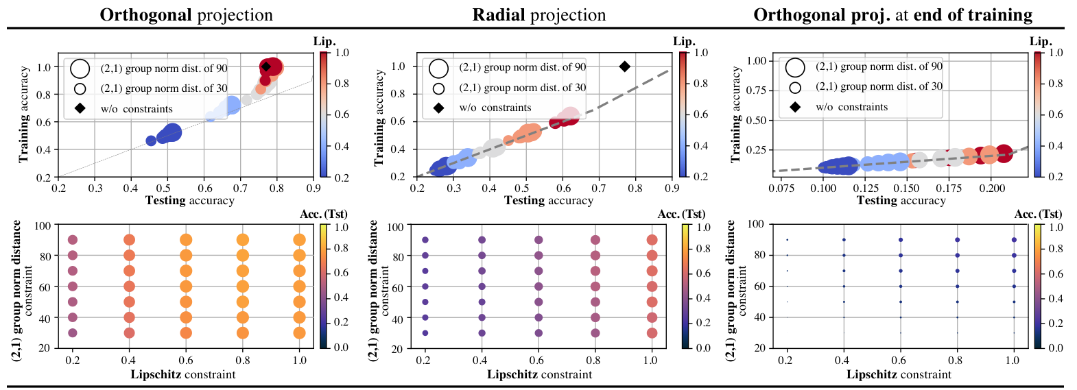
Refer to caption
Figure 7: Comparison of different projection techniques for ResNet18 models trained on CIFAR10. Best-viewed in color.

B.3 Comparison between constrained and unconstrained models beyond testing error

So far, we have analyzed to which extent the weights of neural networks can be constrained without a loss of testing accuracy. In particular, we have identified the maximal constraint strength (i.e., the operating point) such that the testing error of the constrained models is on a par with the one of unconstrained models. However, this does not imply that constrained models and unconstrained ones can be used interchangeably, as they might differ in other aspects. In this section, we will study how pronounced such differences are with respect to (i) biases to particular classes, (ii) susceptibility to adversarial attacks, and (iii) compressibility in terms of the number of weights (via weight pruning).

For the evaluation, we use 25 unconstrained and 25 constrained models trained on CIFAR100, with the same architecture and optimization hyperparameters as listed in the main text, i.e., Section 4. As constraint strength, we choose a layer-wise Lipschitz constant of 0.8 and a distance constraint of 70.

B.3.1 Biases to particular classes

For each of the 50 models, we counted how often each class is predicted on the testing data, which consists of 100 images per class. If there are no biases to particular classes, the counts should be distributed around this value with preferably small spread. Fig. 8 visualizes the results. We immediately see, that for the unconstrained models, the predictions per class are more uniformly distributed with the average class close to 100 and small standard deviations. In contrast, for the constrained models, the standard deviations are much larger. Most striking is the peak at class index 21, indicating that the constrained models are indeed biased to this particular class (chimpanzee). In fact, only one of the 25 models predicted this class less than 100 times. Notably, the unconstrained models are also biased towards this class, as the error region of (mean ±\pm standard deviation) does not contain 100. Overall, there are more favored/disfavored classes for the unconstrained models (32 vs. only 5 for the constrained models), but for the constrained models, the biases are more pronounced.

Figure 8: Prediction frequencies per class index on the testing portion of CIFAR100, averaged over the predictions of 25 constrained and 25 unconstrained (vanilla) ResNet18 models. Best-viewed in color.

B.3.2 Susceptibility to adversarial attacks

We tested several adversarial attacks (FGSM, FGM, L2PGD, LinfPGD, L2DeepFool, L2AdditiveGaussianNoise, L2AdditiveUniformNoise, L2ContrastReduction, GaussianBlur) using the foolbox [39] Python package. To compare constrained vs. unconstrained models, we extract 1024 images from the testing data, which are correctly classified by all 50 models (25 constrained models, 25 unconstrained models) on which the attacks are evaluated. The fraction of correctly classified images for increasing attack strengths is visualized in Fig. 9. As can be seen from the figure, constrained models are less susceptible to the gradient-based attacks FGSM, FGM, L2PGD, and LinfPGD. For L2DeepFool, contrast reduction (L2ContrastReductionAttack) and Gaussian blur (GaussianBlurAttack), constrained and unconstrained models are equally affected. To our surprise, the constrained models more vulnerable to additive Gaussian and uniform noise.

Figure 9: Results of running several adversarial attacks against constrained and unconstrained ResNet18 models on CIFAR100 across varying attack strengths (xx-axis). Each solid line represents one trained model, the dashed lines represent the medians. The yy-axis shows the fraction of correctly classified images that remain correct as attack strength increases. Best-viewed in color.

B.3.3 Compressibility via weight pruning

We measure compressibility for global (unstructured) l1l_{1} weight pruning. This simple pruning technique identifies a predefined fraction of a model’s parameters (i.e., elements of the weight tensors/matrices) and sets them to zero. No subsequent fine-tuning steps were performed.

Figure 10: Results of global (unstructured) l1l_{1} weight pruning on 25 constrained and 25 unconstrained ResNet18 models. Each solid line represents one trained model. Best-viewed in color.

As illustrated in Fig. 10, unconstrained models are less affected by this pruning technique than constrained models. Yet, constrained models can still be pruned, and, in the range of pruning strengths 0 to 0.15, the median testing accuracy drops only marginally for both model types. Only at larger pruning strengths do differences between the model types become visible. If we consider a median testing accuracy of 46%, resp. 45%, to be acceptable, then this threshold allows for pruning 20%, resp. 30%, of the weights of constrained models and 30%, resp 40%, of the unconstrained models. Of course, the pruned models might not satisfy the constraints anymore. In particular, the distance constraint gets violated, as with increasing constraint strength, the distance to initialization converges to the norm of the initialization. Typically, the latter is already larger than the distance constraint (of 70). Thus, when combining norm constraints with weight pruning, constraining the distance with respect to the zero weight appears to be more sensible. This can be done, as the distance constraint in Theorem 3.5 is not required to be with respect to the initialization; it can be chosen relative to any reference weight as long as the reference weight does not depend on the training data.

B.4 Hardware resources

All experiments were run on an Ubuntu Linux 20.04.4 LTS system with 128 GB of main memory, an Intel®Core™ i9-10980XE processor and two NVIDIA GeForce RTX 3090 graphics cards (24 GB memory, CUDA 11.4, driver version 470.129.06). All models are implemented in Pytorch (v1.10).

Appendix C Proofs

In the following sections, we present proofs for the theoretical results listed in the manuscript as well as additional supplementary results.

C.1 Preliminaries

In terms of notation, we consider spaces ℱ\mathcal{F} of functions f:(𝒳,‖⋅‖𝒳)→(𝒴,‖⋅‖𝒴)f\colon(\mathcal{X},\left\lVert\cdot\right\rVert_{\mathcal{X}})\to(\mathcal{Y},\left\lVert\cdot\right\rVert_{\mathcal{Y}}) between normed spaces. We write Lip(f) = sup_x_1, x_2 ∈X ‖ f(x 1 )- f(x 2 ) ‖ Y ‖ x 1 -x 2 ‖ X and Lip(F) = sup_f∈F Lip(f) for the Lipschitz constant of ff and the supremal Lipschitz constant of ℱ\mathcal{F}, respectively. For the remainder of the section, all function spaces ℱ\mathcal{F} will have bounded Lipschitz constants Lip⁡(ℱ)<∞\Lip(\mathcal{F})<\infty. Such function spaces are vector spaces, where addition and scalar multiplication are defined pointwise via the vector space structure on 𝒴\mathcal{Y}, i.e., (f+g):x↦f⁡(x)+g⁡(x)(f+g)\colon x\mapsto f(x)+g(x) and (α​f):x↦α​f​(x)(\alpha f)\colon x\mapsto\alpha f(x).

We equip ℱ\mathcal{F} with a data-dependent norm, defined below.

Definition C.1.

Let ℱ\mathcal{F} be a space of functions f:(𝒳,‖⋅‖𝒳)→(𝒴,‖⋅‖𝒴)f:(\mathcal{X},\left\lVert\cdot\right\rVert_{\mathcal{X}})\to(\mathcal{Y},\left\lVert\cdot\right\rVert_{\mathcal{Y}}) between normed spaces. The data-dependent norm, denoted as ‖⋅‖X\left\lVert\cdot\right\rVert_{X}, on ℱ\mathcal{F} restricted to X=(x1​…,xn)∈𝒳nX=\left(x_{1}\dots,x_{n}\right)\in\mathcal{X}^{n}, i.e., ℱ|X\mathcal{F}|_{X}, is defined as

‖f‖X=∑i=1n‖f⁡(xi)‖𝒴2.\left\lVert f\right\rVert_{X}=\sqrt{\sum_{i=1}^{n}\left\lVert f(x_{i})\right\rVert_{\mathcal{Y}}^{2}}\kern 4.25006pt. (43)
Remark C.2.

This norm is a seminorm on ℱ\mathcal{F} and a norm on ℱ|X={f|{x1,…,xn}:f∈ℱ}\mathcal{F}|_{X}=\{f|_{\left\{x_{1},\dots,x_{n}\right\}}:~f\in\mathcal{F}\}. If f∈ℱf\in\mathcal{F} has norm ‖f‖X=0\left\lVert f\right\rVert_{X}=0, then it holds that ∀i:f⁡(xi)=0\forall i:f(x_{i})=0. Thus, ff is the zero element in ℱ|X\mathcal{F}|_{X}, but not necessarily the zero element in ℱ\mathcal{F}, as there might exist v∈𝒳∖{x1,…,xn}v\in\mathcal{X}\setminus\left\{x_{1},\dots,x_{n}\right\} with f⁡(v)≠0f(v)\neq 0.

Two fundamental properties concerning compositions of functions are worth pointing out:

‖f∘g‖X=‖f‖g⁡(X)and‖f∘g−f∘h‖X≤Lip⁡(f)​‖g−h‖X.\displaystyle\left\lVert f\circ g\right\rVert_{X}=\left\lVert f\right\rVert_{g(X)}\hskip 17.00024pt\text{and}\hskip 17.00024pt\left\lVert f\circ g-f\circ h\right\rVert_{X}\leq\Lip(f)\left\lVert g-h\right\rVert_{X}\kern 4.25006pt. (44)

Further, we recall the definition of covering numbers.

Definition C.3.

Let (ℋ,‖⋅‖)(\mathcal{H},\left\lVert\cdot\right\rVert) be a normed space, S⊂ℋS\subset\mathcal{H} and ϵ>0\epsilon>0. We call any subset U⊂SU\subset S an internal ϵ\epsilon-cover of SS if for every s∈Ss\in S there exists u∈Uu\in U such that ‖s−u‖≤ϵ\left\lVert s-u\right\rVert\leq\epsilon. The internal covering number 𝒩int​(ℋ,ϵ,‖⋅‖)\mathcal{N}^{\text{int}}(\mathcal{H},\epsilon,\left\lVert\cdot\right\rVert) is the cardinality of the smallest internal ϵ\epsilon-cover of SS, i.e.,

𝒩int​(S,ϵ,‖⋅‖)=min⁡({|U|:U is an internal ϵ-cover of S})\mathcal{N}^{\text{int}}(S,\epsilon,\left\lVert\cdot\right\rVert)=\min\left(\left\{|U|:~\text{U is an internal $\epsilon$-cover of $S$}\right\}\right)\kern 4.25006pt (45)

Dropping the requirement U⊂SU\subset S, we analogously define external ϵ\epsilon-covers U⊂ℋU\subset\mathcal{H} and external covering numbers 𝒩ext​(S,ϵ,‖⋅‖)\mathcal{N}^{\text{ext}}(S,\epsilon,\left\lVert\cdot\right\rVert).

In the manuscript, if not stated otherwise, covers will always be internal and covering numbers will be denoted as 𝒩=𝒩int\mathcal{N}=\mathcal{N}^{\text{int}}.

Internal and external covering numbers are related via the following chain of inequalities:

𝒩ext​(S,ϵ,‖⋅‖)≤𝒩int​(S,ϵ,‖⋅‖)≤𝒩ext​(S,ϵ/2,‖⋅‖).\mathcal{N}^{\text{ext}}(S,\epsilon,\left\lVert\cdot\right\rVert)\leq\mathcal{N}^{\text{int}}(S,\epsilon,\left\lVert\cdot\right\rVert)\leq\mathcal{N}^{\text{ext}}(S,\epsilon/2,\left\lVert\cdot\right\rVert)\kern 4.25006pt. (46)

The first inequality follows directly from the definition of covering numbers; the second one follows from the triangle inequality. Furthermore, for any subset T⊂ST\subset S, it holds that

𝒩ext​(T,ϵ,‖⋅‖)≤𝒩ext​(S,ϵ,‖⋅‖).\mathcal{N}^{\text{ext}}(T,\epsilon,\left\lVert\cdot\right\rVert)\leq\mathcal{N}^{\text{ext}}(S,\epsilon,\left\lVert\cdot\right\rVert)\kern 4.25006pt. (47)

Notably, this is not true for internal coverings. For example, the unit ball in ℝd\mathbb{R}^{d} defines an internal cover of itself, whereas an annulus cannot be covered internally with only one ball of radius 11.

C.2 Single-layer covering number bounds

This section contains the covering number bounds for single convolutional layers. For simplicity, we will first present the special case of the single-layer covering number bound for 1D convolutions with one channel, stride 1, odd kernel size and input size preserving (zero) padding. The proof of the general case then follows along the same line of arguments, but is more tedious, due to the additional notation and subindices.

Let X=(x1,…,xn)∈𝒳nX=(x_{1},\dots,x_{n})\in\mathcal{X}^{n} with xi∈𝒳=ℝhx_{i}\in\mathcal{X}=\mathbb{R}^{h}. Further, let K∈ℝkK\in\mathbb{R}^{k}, with kk odd, be a convolutional kernel and ϕK:ℝh→ℝh\phi_{K}:\mathbb{R}^{h}\to\mathbb{R}^{h} the corresponding convolutional map, which is defined coordinate-wise as

[ϕK​(x)]i=∑α=−k−12k−12Kα​xi+α​𝟙i+α∈[1,h].[\phi_{K}(x)]_{i}=\sum_{\alpha=-\frac{k-1}{2}}^{\frac{k-1}{2}}K_{\alpha}\,x_{i+\alpha}\mathbbm{1}_{i+\alpha\in[1,h]}\kern 4.25006pt. (48)

For the norm of the data XX, we write

‖X‖=∑i=1n‖xi‖2.\left\lVert X\right\rVert=\sqrt{\sum_{i=1}^{n}\left\lVert x_{i}\right\rVert^{2}}\kern 4.25006pt. (49)

Our covering number bounds hinge on the seminal Maurey sparsification lemma. We state one variant, see [3, Lemma A.6].

Lemma C.4 (Maurey sparsification lemma).

Fix a Hilbert space ℋ\mathcal{H} with norm ‖⋅‖\left\lVert\cdot\right\rVert. Let U∈ℋU\in\mathcal{H} be given with representation U=∑i=1dαi​ViU=\sum_{i=1}^{d}\alpha_{i}V_{i} where Vi∈ℋV_{i}\in\mathcal{H}, α∈ℝ≥0d∖{0}\alpha\in\mathbb{R}^{d}_{\geq 0}\setminus\left\{0\right\} and ∑i|αi|≤1\sum_{i}|\alpha_{i}|\leq 1. Then, for any positive integer mm, there exists a choice of non-negative integers (m1,…,md)(m_{1},\dots,m_{d}) with ∑imi=m\sum_{i}m_{i}=m, such that

‖U−1m​∑i=1dmi​Vi‖2≤1m​maxi=1,…,d​‖Vi‖2.\left\lVert U-\frac{1}{m}\sum_{i=1}^{d}m_{i}V_{i}\right\rVert^{2}\leq\frac{1}{m}\max_{i=1,\dots,d}\left\lVert V_{i}\right\rVert^{2}\kern 4.25006pt. (50)
Theorem C.5 (Single-layer covering number bound – Simple 1D variant).

Let b>0b>0, kk odd and let ℱ={ϕK|K∈ℝk,‖K‖1≤b}\mathcal{F}=\{\phi_{K}|~K\in\mathbb{R}^{k},\left\lVert K\right\rVert_{1}\leq b\} be the set of 1D convolutions determined by kernels K∈ℝkK\in\mathbb{R}^{k} with ‖K‖1≤b\left\lVert K\right\rVert_{1}\leq b. For any X=(x1,…,xn)∈𝒳n=ℝn×hX=(x_{1},\dots,x_{n})\in\mathcal{X}^{n}=\mathbb{R}^{n\times h} and ϵ>0\epsilon>0, the covering number 𝒩⁡(ℱ,ϵ,‖⋅‖X)\mathcal{N}(\mathcal{F},\epsilon,\left\lVert\cdot\right\rVert_{X}) satisfies

log⁡𝒩⁡(ℱ,ϵ,‖⋅‖X)≤⌈‖X‖2​b2ϵ2⌉​log⁡(2​k)\log\mathcal{N}(\mathcal{F},\epsilon,\left\lVert\cdot\right\rVert_{X})\leq\left\lceil\frac{\left\lVert X\right\rVert^{2}b^{2}}{\epsilon^{2}}\right\rceil\log(2k) (51)

and

log⁡𝒩⁡(ℱ,ϵ,‖⋅‖X)≤(2​k−1)​log⁡(1+⌈‖X‖2​b2ϵ2⌉).\log\mathcal{N}(\mathcal{F},\epsilon,\left\lVert\cdot\right\rVert_{X})\leq(2k-1)\log\left(1+\left\lceil\frac{\left\lVert X\right\rVert^{2}b^{2}}{\epsilon^{2}}\right\rceil\right)\kern 4.25006pt. (52)
Proof.

We rewrite the coordinate-wise definition of the 1D convolutional operation from Eq. 48 with unit stride as

[ϕK​(x)]i=∑j=1h(∑α=−k−12k−12𝟙j=α+i​Kα)⏟=Mi​j​xj=∑j=1hMi​j​xj.\displaystyle[\phi_{K}(x)]_{i}=\sum_{j=1}^{h}\underbrace{\left(\sum_{\alpha=-\frac{k-1}{2}}^{\frac{k-1}{2}}\mathbbm{1}_{j=\alpha+i}\,K_{\alpha}\right)}_{=M_{ij}}x_{j}=\sum_{j=1}^{h}M_{ij}x_{j}\kern 4.25006pt.

Thus, convolution is a linear map parametrized by a matrix M∈ℝh×hM\in\mathbb{R}^{h\times h} with entries M_ij = ∑_α=- k-1 2 ^ k-1 2 1_j = α+ i  K_α . In particular, we can write M=∑α=−(k−1)/2(k−1)/2KαM(α)M=\sum_{\alpha=-(k-1)/2}^{(k-1)/2}K_{\alpha}M^{(\alpha)} with Mi​j(α)=𝟙j−i=αM^{(\alpha)}_{ij}=\mathbbm{1}_{j-i=\alpha} and note that for every x∈ℝhx\in\mathbb{R}^{h} and every α\alpha, we have ‖M^(α)x‖≤‖x‖ .

For example, if h=5h=5 and k=3k=3, we have

M=(K0K1000K−1K0K1000K−1K0K1000K−1K0K1000K−1K0),\displaystyle M=\begin{pmatrix}K_{0}&K_{1}&0&0&0\\ K_{-1}&K_{0}&K_{1}&0&0\\ 0&K_{-1}&K_{0}&K_{1}&0\\ 0&0&K_{-1}&K_{0}&K_{1}\\ 0&0&0&K_{-1}&K_{0}\end{pmatrix},
M(−1)=(0000010000010000010000010),M(0)=(1000001000001000001000001),M(1)=(0100000100000100000100000).\displaystyle M^{(-1)}=\begin{pmatrix}0&0&0&0&0\\ 1&0&0&0&0\\ 0&1&0&0&0\\ 0&0&1&0&0\\ 0&0&0&1&0\end{pmatrix},~~M^{(0)}=\begin{pmatrix}1&0&0&0&0\\ 0&1&0&0&0\\ 0&0&1&0&0\\ 0&0&0&1&0\\ 0&0&0&0&1\end{pmatrix},~~M^{(1)}=\begin{pmatrix}0&1&0&0&0\\ 0&0&1&0&0\\ 0&0&0&1&0\\ 0&0&0&0&1\\ 0&0&0&0&0\end{pmatrix}\kern 4.25006pt.

In summary, we have ϕ_K(x) =∑_α=-(k-1)/2^(k-1)/2 K_α M^(α) x = ∑_α=-(k-1)/2^(k-1)/2 K α b b M^(α) x  . By assumption, we have ∑α|Kαb|=‖K‖1b≤1\sum_{\alpha}\left|\frac{K_{\alpha}}{b}\right|=\frac{\left\lVert K\right\rVert_{1}}{b}\leq 1 and so we can instantiate Maurey’s sparsification lemma (Eq. 50) on the Hilbert space (ℱ|X,‖⋅‖X)(\mathcal{F}|_{X},\left\lVert\cdot\right\rVert_{X}) for {V1,…V2​d}={x↦±bM(α)x|α=1,…,d}⊂ℱ\left\{V_{1},\dots V_{2d}\right\}=\left\{x\mapsto\pm bM^{(\alpha)}x|~\alpha=1,\dots,d\right\}\subset\mathcal{F}. As a consequence, for any convolutional kernel K∈ℝkK\in\mathbb{R}^{k} and any m∈ℕm\in\mathbb{N}, there exist (m1,…,m2​d)(m_{1},\dots,m_{2d}) with ∑i=12​dmi=m\sum_{i=1}^{2d}m_{i}=m such that

‖ϕK−1m​∑i=12​dmi​Vi‖X2≤1m​maxi=1​…,2​d​‖Vi‖X2.\left\lVert\phi_{K}-\frac{1}{m}\sum_{i=1}^{2d}m_{i}V_{i}\right\rVert_{X}^{2}\leq\frac{1}{m}\max_{i=1\dots,2d}\left\lVert V_{i}\right\rVert_{X}^{2}\kern 4.25006pt.

Thus, for fixed ϵ>0\epsilon>0, if we choose m∈ℕm\in\mathbb{N} such that 1m​maxi​‖Vi‖X2≤ϵ2\frac{1}{m}\max_{i}\left\lVert V_{i}\right\rVert_{X}^{2}\leq\epsilon^{2}, then the solutions (in mim_{i}), of ∑i=12​dmi=m\sum_{i=1}^{2d}m_{i}=m, define an ϵ\epsilon-cover

{1m∑i=12​dmiVi|mi∈ℕ≥0,∑i=12​dmi=m}⊂ℱ.\left\{\frac{1}{m}\sum_{i=1}^{2d}m_{i}V_{i}|~m_{i}\in\mathbb{N}_{\geq 0},~\sum_{i=1}^{2d}m_{i}=m\right\}\subset\mathcal{F}\kern 4.25006pt.

As the number of non-negative 2​d2d-tuples that add up to mm is equal to77 7 This number equals the number of possibilities to separate mm objects by 2​d−12d-1 delimiters. This corresponds to choosing 2​d−12d-1 elements (position of delimiters) from a set of m+2​d−1m+2d-1 elements (objects + delimiters). N(m,d) = ( m + 2d -1 2d-1 )  , this means that ℱ\mathcal{F} has an ϵ\epsilon-cover of cardinality at most N⁡(m,d)N(m,d), and so 𝒩⁡(ℱ,ϵ,‖⋅‖X)≤N⁡(m,d)\mathcal{N}(\mathcal{F},\epsilon,\left\lVert\cdot\right\rVert_{X})\leq N(m,d).

Since for all i∈{1,…,2​d}i\in\{1,\dots,2d\}, the norms ‖Vi‖X2\left\lVert V_{i}\right\rVert_{X}^{2} satisfy

‖Vi‖X2=‖b​M(αi)‖X2=b2​∑j=1n‖M(αi)​xj‖2≤b2​∑j=1n‖xj‖2=b2​‖X‖2,\left\lVert V_{i}\right\rVert_{X}^{2}=\left\lVert bM^{(\alpha_{i})}\right\rVert_{X}^{2}=b^{2}\sum_{j=1}^{n}\left\lVert M^{(\alpha_{i})}x_{j}\right\rVert^{2}\leq b^{2}\sum_{j=1}^{n}\left\lVert x_{j}\right\rVert^{2}=b^{2}\left\lVert X\right\rVert^{2}\kern 4.25006pt,

we can choose ℕ∋m=⌈b2​‖X‖2ϵ2⌉\mathbb{N}\ni m=\left\lceil\frac{b^{2}\left\lVert X\right\rVert^{2}}{\epsilon^{2}}\right\rceil.

The theorem then follows from two particular bounds on N⁡(m,d)N(m,d), see Lemma C.24. These are ( m + 2d -1 2d-1 ) ≤(2d)^m , which implies Eq. 51, and ( m + 2d -1 2d-1 ) ≤(1+m)^2d-1  , which implies Eq. 52. ∎

Remark C.6.

The definition of the convolution operation in Eq. 48 corresponds to convolutional layers with zero-padding, such that the dimensionality hh of the data remains unchanged (i.e., input-size preserving). The covering bound equally holds for other types of padding, corresponding to other matrices M(α)M^{(\alpha)}, as long as

‖M(α)​x‖≤x\left\lVert M^{(\alpha)}x\right\rVert\leq x

for all xx. In particular, it holds for convolutional layers with circular padding, where the matrices M(α)M^{(\alpha)} become permutation matrices.

Next, we study the general case of 2D multi-channel convolutions with strides. To that end, let ϕK\phi_{K} be the map determined by a weight tensor K∈ℝcout×cin×kh×kwK\in\mathbb{R}^{c_{\textit{out}}\times c_{\textit{in}}\times k_{h}\times k_{w}}, where cout,cinc_{\textit{out}},c_{\textit{in}} denote the number of output and input channels, resp., and (kh,kw)(k_{h},k_{w}) is the spatial extension of the kernel. For input images x∈ℝcin×h×wx\in\mathbb{R}^{c_{\textit{in}}\times h\times w}, convolution ϕK,(sh,sw):ℝcin×h×w→ℝcin×⌈h/sh⌉×⌈w/sw⌉\phi_{K,(s_{h},s_{w})}:\mathbb{R}^{c_{\textit{in}}\times h\times w}\to\mathbb{R}^{c_{\textit{in}}\times\left\lceil h/s_{h}\right\rceil\times\left\lceil w/s_{w}\right\rceil} with strides (sh,sw)(s_{h},s_{w}) is defined coordinate-wise as

[ϕK,(sh,sw)(x)]σ​μ​ν=∑r=1cin∑i=⌊−kh−12⌋⌊kh−12⌋∑j=⌊−kw−12⌋⌊kw−12⌋\displaystyle[\phi_{K,(s_{h},s_{w})}(x)]_{\sigma\mu\nu}=\sum_{r=1}^{c_{\textit{in}}}\sum_{i=\lfloor-\frac{k_{h}-1}{2}\rfloor}^{\lfloor\frac{k_{h}-1}{2}\rfloor}\sum_{j=\lfloor-\frac{k_{w}-1}{2}\rfloor}^{\lfloor\frac{k_{w}-1}{2}\rfloor} Kσ​r​i​j​xr,1+sh​(μ−1)+i,1+sw​(ν−1)+j\displaystyle K_{\sigma rij}\,x_{r,1+s_{h}(\mu-1)+i,1+s_{w}(\nu-1)+j} (53)
⋅𝟙1+sh​(μ−1)+i∈[1,h]​𝟙1+sw​(ν−1)+j∈[1,w]\displaystyle\hskip 17.00024pt\hskip 17.00024pt\cdot\mathbbm{1}_{1+s_{h}(\mu-1)+i\in[1,h]}\mathbbm{1}_{1+s_{w}(\nu-1)+j\in[1,w]}
Theorem C.7 (Single-layer covering number bound – General case).

Let b>0b>0. Define the class of (sh,sw)(s_{h},s_{w})-strided 2D convolutions parametrized by tensors K∈ℝcout×cin×kh×kwK\in\mathbb{R}^{c_{\textit{out}}\times c_{\textit{in}}\times k_{h}\times k_{w}} with W=cout​cin​kh​kwW={c_{\textit{out}}c_{\textit{in}}k_{h}k_{w}} parameters and (2,12,1) group norm ‖K‖2,1≤b\left\lVert K\right\rVert_{2,1}\leq b as

ℱ={ϕK,(sh,sw)|K∈ℝcout×cin×kh×kw,‖K‖2,1≤b}.\mathcal{F}=\{\phi_{K,(s_{h},s_{w})}~|~K\in\mathbb{R}^{c_{\textit{out}}\times c_{\textit{in}}\times k_{h}\times k_{w}},\left\lVert K\right\rVert_{2,1}\leq b\}\kern 4.25006pt.

Then, for any X=(x1,…,xn)∈ℝn×cin×h×wX=(x_{1},\dots,x_{n})\in\mathbb{R}^{n\times c_{\textit{in}}\times h\times w} and ϵ>0\epsilon>0, the covering number 𝒩⁡(ℱ,ϵ,‖⋅‖X)\mathcal{N}(\mathcal{F},\epsilon,\left\lVert\cdot\right\rVert_{X}) satisfies

log⁡𝒩⁡(ℱ,ϵ,‖⋅‖X)≤⌈‖X‖2​b2ϵ2⌉​log⁡(2​W)\log\mathcal{N}(\mathcal{F},\epsilon,\left\lVert\cdot\right\rVert_{X})\leq\left\lceil\frac{\left\lVert X\right\rVert^{2}b^{2}}{\epsilon^{2}}\right\rceil\log(2W) (54)

and

log⁡𝒩⁡(ℱ,ϵ,‖⋅‖X)≤(2​W−1)​log⁡(1+⌈‖X‖2​b2ϵ2⌉).\log\mathcal{N}(\mathcal{F},\epsilon,\left\lVert\cdot\right\rVert_{X})\leq(2W-1)\log\left(1+\left\lceil\frac{\left\lVert X\right\rVert^{2}b^{2}}{\epsilon^{2}}\right\rceil\right)\kern 4.25006pt. (55)
Remark C.8.

Recall that convolution with kernel size 1 and input size 1 is a linear map on the input channels, determined by the matrix MK=K⋅⋅11M_{K}=K_{\cdot\cdot 11}. In this situation, the convolutional layer reduces to a fully-connected layer and our first bound reduces to [3, Lemma 3.2].

Proof.

The proof is quite similar to the one of the special case in Theorem C.5. Recall, that the convolution operation is defined coordinate-wise in Eq. 53. Using identities of the form 𝟙t∈{1,…,n}=∑i=1n𝟙i=t\mathbbm{1}_{t\in\left\{1,\dots,n\right\}}=\sum_{i=1}^{n}\mathbbm{1}_{i=t}, we write

[ϕK,(sh,sw)​(x)]σ​μ​ν=\displaystyle[\phi_{K,(s_{h},s_{w})}(x)]_{\sigma\mu\nu}=
∑α=1cin∑β=1h∑γ=1wxα​β​γ​(∑p=1cout∑r=1cin∑i=⌊−kh−12⌋⌊kh−12⌋∑j=⌊−kw−12⌋⌊kw−12⌋Kp​r​i​j​𝟙p=σ​𝟙α=r​𝟙β=1+sh​(μ−1)+i​𝟙γ=1+sw​(ν−1)+j⏟=[M(p,r,i,j)]σ​μ​να​β​γ)\displaystyle\sum_{\alpha=1}^{c_{\textit{in}}}\sum_{\beta=1}^{h}\sum_{\gamma=1}^{w}x_{\alpha\beta\gamma}\!\left(\!\sum_{p=1}^{c_{\textit{out}}}\!\sum_{r=1}^{c_{\textit{in}}}\!\sum_{i=\lfloor-\frac{k_{h}-1}{2}\rfloor}^{\lfloor\frac{k_{h}-1}{2}\rfloor}\sum_{j=\lfloor-\frac{k_{w}-1}{2}\rfloor}^{\lfloor\frac{k_{w}-1}{2}\rfloor}\!\!\!\!\!K_{prij}\underbrace{\mathbbm{1}_{p=\sigma}\mathbbm{1}_{\alpha=r}\mathbbm{1}_{\beta=1+s_{h}(\mu-1)+i}\mathbbm{1}_{\gamma=1+s_{w}(\nu-1)+j}}_{=[M^{(p,r,i,j)}]^{\alpha\beta\gamma}_{\sigma\mu\nu}}\!\right)

and condense this into

[ϕK,(sh,sw)​(x)]σ​μ​ν\displaystyle[\phi_{K,(s_{h},s_{w})}(x)]_{\sigma\mu\nu} =∑α=1cin∑β=1h∑γ=1wxα​β​γ​(∑p=1cout∑r=1cin∑i=⌊−kh−12⌋⌊kh−12⌋∑j=⌊−kw−12⌋⌊kw−12⌋Kp​r​i​j​[M(p,r,i,j)]σ​μ​να​β​γ)⏟=Mσ​μ​να​β​γ\displaystyle=\sum_{\alpha=1}^{c_{\textit{in}}}\sum_{\beta=1}^{h}\sum_{\gamma=1}^{w}x_{\alpha\beta\gamma}\underbrace{\left(\sum_{p=1}^{c_{\textit{out}}}\sum_{r=1}^{c_{\textit{in}}}\sum_{i=\lfloor-\frac{k_{h}-1}{2}\rfloor}^{\lfloor\frac{k_{h}-1}{2}\rfloor}\sum_{j=\lfloor-\frac{k_{w}-1}{2}\rfloor}^{\lfloor\frac{k_{w}-1}{2}\rfloor}K_{prij}[M^{(p,r,i,j)}]^{\alpha\beta\gamma}_{\sigma\mu\nu}\right)}_{=M^{\alpha\beta\gamma}_{\sigma\mu\nu}}\kern 4.25006pt
=∑α=1cin∑β=1h∑γ=1wxα​β​γ​Mσ​μ​να​β​γ.\displaystyle=\sum_{\alpha=1}^{c_{\textit{in}}}\sum_{\beta=1}^{h}\sum_{\gamma=1}^{w}x_{\alpha\beta\gamma}M^{\alpha\beta\gamma}_{\sigma\mu\nu}\kern 4.25006pt.

Thus, the convolution is a multilinear map ℝcin×h×w→ℝcin×⌈h/sh⌉×⌈w/sw⌉\mathbb{R}^{c_{\textit{in}}\times h\times w}\to\mathbb{R}^{c_{\textit{in}}\times\left\lceil h/s_{h}\right\rceil\times\left\lceil w/s_{w}\right\rceil} parametrized by

M\displaystyle M =∑p=1cout∑r=1cin∑i=⌊−kh−12⌋⌊kh−12⌋∑j=⌊−kw−12⌋⌊kw−12⌋Kp​r​i​j​M(p,r,i,j)\displaystyle=\sum_{p=1}^{c_{\textit{out}}}\sum_{r=1}^{c_{\textit{in}}}\sum_{i=\lfloor-\frac{k_{h}-1}{2}\rfloor}^{\lfloor\frac{k_{h}-1}{2}\rfloor}\sum_{j=\lfloor-\frac{k_{w}-1}{2}\rfloor}^{\lfloor\frac{k_{w}-1}{2}\rfloor}K_{prij}M^{(p,r,i,j)}
=∑p=1cout∑r=1cin∑i=⌊−kh−12⌋⌊kh−12⌋∑j=⌊−kw−12⌋⌊kw−12⌋(Kp​r​i​j​‖X⋅r⋅⋅‖‖X‖​b)​(‖X‖​b‖X⋅r⋅⋅‖​M(p,r,i,j)).\displaystyle=\sum_{p=1}^{c_{\textit{out}}}\sum_{r=1}^{c_{\textit{in}}}\sum_{i=\lfloor-\frac{k_{h}-1}{2}\rfloor}^{\lfloor\frac{k_{h}-1}{2}\rfloor}\sum_{j=\lfloor-\frac{k_{w}-1}{2}\rfloor}^{\lfloor\frac{k_{w}-1}{2}\rfloor}\left(K_{prij}\frac{\left\lVert X_{\cdot r\cdot\cdot}\right\rVert}{\left\lVert X\right\rVert b}\right)\left(\frac{\left\lVert X\right\rVert b}{\left\lVert X_{\cdot r\cdot\cdot}\right\rVert}M^{(p,r,i,j)}\right)\kern 4.25006pt.

Since

‖Kp​r​i​j​‖X⋅r⋅⋅‖‖X‖​b‖1\displaystyle\left\lVert K_{prij}\frac{\left\lVert X_{\cdot r\cdot\cdot}\right\rVert}{\left\lVert X\right\rVert b}\right\rVert_{1} =1‖X‖​b∑p=1cout∑i=⌊−kh−12⌋⌊kh−12⌋∑j=⌊−kw−12⌋⌊kw−12⌋(∑r=1cin|Kp​r​i​j|‖X⋅r⋅⋅‖)\displaystyle=\frac{1}{\left\lVert X\right\rVert b}\sum_{p=1}^{c_{\textit{out}}}\sum_{i=\lfloor-\frac{k_{h}-1}{2}\rfloor}^{\lfloor\frac{k_{h}-1}{2}\rfloor}\sum_{j=\lfloor-\frac{k_{w}-1}{2}\rfloor}^{\lfloor\frac{k_{w}-1}{2}\rfloor}\left(\sum_{r=1}^{c_{\textit{in}}}|K_{prij}|\left\lVert X_{\cdot r\cdot\cdot}\right\rVert\right)
≤1‖X‖​b​∑p=1cout∑i=⌊−kh−12⌋⌊kh−12⌋∑j=⌊−kw−12⌋⌊kw−12⌋(∑r=1cin|Kp​r​i​j|2)1/2​(∑r=1cin‖X⋅r⋅⋅‖2)1/2⏟=‖X‖\displaystyle\leq\frac{1}{\left\lVert X\right\rVert b}\sum_{p=1}^{c_{\textit{out}}}\sum_{i=\lfloor-\frac{k_{h}-1}{2}\rfloor}^{\lfloor\frac{k_{h}-1}{2}\rfloor}\sum_{j=\lfloor-\frac{k_{w}-1}{2}\rfloor}^{\lfloor\frac{k_{w}-1}{2}\rfloor}\left(\sum_{r=1}^{c_{\textit{in}}}|K_{prij}|^{2}\right)^{1/2}\underbrace{\left(\sum_{r=1}^{c_{\textit{in}}}\left\lVert X_{\cdot r\cdot\cdot}\right\rVert^{2}\right)^{1/2}}_{=\left\lVert X\right\rVert}
=1b​∑p=1cout∑i=⌊−kh−12⌋⌊kh−12⌋∑j=⌊−kw−12⌋⌊kw−12⌋(∑r=1cin|Kp​r​i​j|2)1/2\displaystyle=\frac{1}{b}\sum_{p=1}^{c_{\textit{out}}}\sum_{i=\lfloor-\frac{k_{h}-1}{2}\rfloor}^{\lfloor\frac{k_{h}-1}{2}\rfloor}\sum_{j=\lfloor-\frac{k_{w}-1}{2}\rfloor}^{\lfloor\frac{k_{w}-1}{2}\rfloor}\left(\sum_{r=1}^{c_{\textit{in}}}|K_{prij}|^{2}\right)^{1/2}
=‖K‖2,1b≤(by assumption)1,\displaystyle=\frac{\left\lVert K\right\rVert_{2,1}}{b}\stackrel{{\scriptstyle\text{(by assumption)}}}{{\leq}}1\kern 4.25006pt,

we can instantiate Maurey’s sparsification lemma (Eq. 50) on the Hilbert space (ℱ|X,‖⋅‖X)(\mathcal{F}|_{X},\left\lVert\cdot\right\rVert_{X}) for

{V1,…,V2​W}={±‖X‖​b‖X⋅r⋅⋅‖M(p,r,i,j)|\displaystyle\left\{V_{1},\dots,V_{2W}\right\}=\Bigg\{\pm\frac{\left\lVert X\right\rVert b}{\left\lVert X_{\cdot r\cdot\cdot}\right\rVert}M^{(p,r,i,j)}~\Bigg|~ p∈{1,…,cout},r∈{1​…,cin},\displaystyle p\in\left\{1,\dots,c_{\textit{out}}\right\},r\in\left\{1\dots,c_{\textit{in}}\right\},
i∈{⌊−kh−12⌋,…,⌊kh−12⌋},\displaystyle i\in\left\{\Bigl\lfloor-\frac{k_{h}-1}{2}\Bigr\rfloor,\dots,\Bigl\lfloor\frac{k_{h}-1}{2}\Bigr\rfloor\right\},
j∈{⌊−kw−12⌋…,⌊kw−12⌋}}.\displaystyle j\in\left\{\Bigl\lfloor-\frac{k_{w}-1}{2}\Bigr\rfloor\dots,\Bigl\lfloor\frac{k_{w}-1}{2}\Bigr\rfloor\right\}\Bigg\}\kern 4.25006pt.

As a consequence, for any convolutional kernel K∈ℝcout×cin×kh×kwK\in\mathbb{R}^{c_{\textit{out}}\times c_{\textit{in}}\times k_{h}\times k_{w}} and any m∈ℕm\in\mathbb{N}, there exist (m1,…,m2​W)(m_{1},\dots,m_{2W}) with ∑i=12​Wmi=m\sum_{i=1}^{2W}m_{i}=m such that

‖ϕOPENK,(sh,sw))−1m​∑i=12​Wmi​Vi‖X2≤1m​maxi​‖Vi‖X2.\left\lVert\phi_{K,(s_{h},s_{w}))}-\frac{1}{m}\sum_{i=1}^{2W}m_{i}V_{i}\right\rVert_{X}^{2}\leq\frac{1}{m}\max_{i}\left\lVert V_{i}\right\rVert_{X}^{2}\kern 4.25006pt.

Thus, for fixed ϵ>0\epsilon>0, if we choose m∈ℕm\in\mathbb{N} such that 1m​maxi​‖Vi‖X2≤ϵ2\frac{1}{m}\max_{i}\left\lVert V_{i}\right\rVert_{X}^{2}\leq\epsilon^{2}, then the solutions in mim_{i} of ∑i=12​Wmi=m\sum_{i=1}^{2W}m_{i}=m, define an ϵ\epsilon-cover

{1m∑i=12​WmiVi|mi∈ℕ≥0,∑i=12​Wmi=m}⊂ℱ.\left\{\frac{1}{m}\sum_{i=1}^{2W}m_{i}V_{i}|~m_{i}\in\mathbb{N}_{\geq 0},~\sum_{i=1}^{2W}m_{i}=m\right\}\subset\mathcal{F}\kern 4.25006pt. (56)

As the number of non-negative 2​W2W-tuples which add up to mm, denoted as N⁡(m,W)N(m,W), is equal to N(m,W)= ( m + 2W -1 2W-1 )  , this means that ℱ\mathcal{F} has an ϵ\epsilon-cover of cardinality at most N⁡(m,W)N(m,W); thus, 𝒩⁡(ℱ,ϵ,‖⋅‖X)≤N⁡(m,W)\mathcal{N}(\mathcal{F},\epsilon,\left\lVert\cdot\right\rVert_{X})\leq N(m,W).

In order to compute the norms ‖Vi‖X2\left\lVert V_{i}\right\rVert_{X}^{2}, we use that for all (p,r,i,j)∈[cout]×[cin]×[kh]×[kw](p,r,i,j)\in[c_{\textit{out}}]\times[c_{\textit{in}}]\times[k_{h}]\times[k_{w}] and for all x∈ℝcin×h×wx\in\mathbb{R}^{c_{\textit{in}}\times h\times w}, it holds that

‖M(p,r,i,j)​x‖2\displaystyle\left\lVert M^{(p,r,i,j)}x\right\rVert^{2} =∑σ,μ,ν[M(p,r,i,j)​x]σ​μ​ν2\displaystyle=\sum_{\sigma,\mu,\nu}[M^{(p,r,i,j)}x]_{\sigma\mu\nu}^{2}
=∑σ,μ,ν(∑α=1cin∑β=1h∑γ=1w[M(p,r,i,j)]σ​μ​να​β​γ​xα​β​γ)2\displaystyle=\sum_{\sigma,\mu,\nu}\left(\sum_{\alpha=1}^{c_{\textit{in}}}\sum_{\beta=1}^{h}\sum_{\gamma=1}^{w}[M^{(p,r,i,j)}]^{\alpha\beta\gamma}_{\sigma\mu\nu}x_{\alpha\beta\gamma}\right)^{2}
=∑σ,μ,ν(∑α=1cin∑β=1h∑γ=1w𝟙p=σ​𝟙α=r​𝟙β=1+sh​(μ−1)+i​𝟙γ=1+sw​(ν−1)+j​xα​β​γ)2\displaystyle=\sum_{\sigma,\mu,\nu}\left(\sum_{\alpha=1}^{c_{\textit{in}}}\sum_{\beta=1}^{h}\sum_{\gamma=1}^{w}\mathbbm{1}_{p=\sigma}\mathbbm{1}_{\alpha=r}\mathbbm{1}_{\beta=1+s_{h}(\mu-1)+i}\mathbbm{1}_{\gamma=1+s_{w}(\nu-1)+j}x_{\alpha\beta\gamma}\right)^{2}
=∑σ,μ,ν(𝟙p=σ​xr,1+sh​(μ−1)+i,1+sw​(ν−1)+j)2\displaystyle=\sum_{\sigma,\mu,\nu}\left(\mathbbm{1}_{p=\sigma}x_{r,1+s_{h}(\mu-1)+i,1+s_{w}(\nu-1)+j}\right)^{2}
=∑μ=1⌈h/sh⌉∑ν=1⌈w/sw⌉(xr,1+sh​(μ−1)+i,1+sw​(ν−1)+j)2\displaystyle=\sum_{\mu=1}^{\left\lceil h/s_{h}\right\rceil}\sum_{\nu=1}^{\left\lceil w/s_{w}\right\rceil}\left(x_{r,1+s_{h}(\mu-1)+i,1+s_{w}(\nu-1)+j}\right)^{2}
=∑β=1h∑γ=1w(xr​β​γ)2​𝟙β≡(1+i)modsh​𝟙γ≡(1+j)modsw\displaystyle=\sum_{\beta=1}^{h}\sum_{\gamma=1}^{w}\left(x_{r\beta\gamma}\right)^{2}\mathbbm{1}_{\beta\equiv(1+i)\!\!\!\!\mod s_{h}}\mathbbm{1}_{\gamma\equiv(1+j)\!\!\!\!\mod s_{w}}
≤∑β=1h∑γ=1w(xr​β​γ)2=‖xr⋅⋅‖2.\displaystyle\leq\sum_{\beta=1}^{h}\sum_{\gamma=1}^{w}\left(x_{r\beta\gamma}\right)^{2}=\left\lVert x_{r\cdot\cdot}\right\rVert^{2}\kern 4.25006pt.

Thus, for any t∈{1,…,2​W}t\in\left\{1,\dots,2W\right\},

‖Vt‖X2=‖±‖X‖​b‖X⋅r⋅⋅‖​M(pt,rt,it,jt)‖X2\displaystyle\left\lVert V_{t}\right\rVert_{X}^{2}=\left\lVert\pm\frac{\left\lVert X\right\rVert b}{\left\lVert X_{\cdot r\cdot\cdot}\right\rVert}M^{(p_{t},r_{t},i_{t},j_{t})}\right\rVert_{X}^{2} =‖X‖2​b2‖X⋅r⋅⋅‖2​∑k=1n‖M(pt,rt,it,jt)​xk‖2\displaystyle=\frac{\left\lVert X\right\rVert^{2}b^{2}}{\left\lVert X_{\cdot r\cdot\cdot}\right\rVert^{2}}\sum_{k=1}^{n}\left\lVert M^{(p_{t},r_{t},i_{t},j_{t})}x_{k}\right\rVert^{2}
≤‖X‖2​b2‖X⋅r⋅⋅‖2∑k=1n‖Xkr⋅⋅‖2=‖X‖2b2,\displaystyle\leq\frac{\left\lVert X\right\rVert^{2}b^{2}}{\left\lVert X_{\cdot r\cdot\cdot}\right\rVert^{2}}\sum_{k=1}^{n}\left\lVert X_{kr\cdot\cdot}\right\rVert^{2}=\left\lVert X\right\rVert^{2}b^{2}\kern 4.25006pt,

and we can choose ℕ∋m=⌈b2​‖X‖2ϵ2⌉\mathbb{N}\ni m=\left\lceil\frac{b^{2}\left\lVert X\right\rVert^{2}}{\epsilon^{2}}\right\rceil to get an ϵ\epsilon-cover of ℱ\mathcal{F} via Eq. 56.

The theorem then follows from two particular bounds on N⁡(m,W)=(m+2​W−12​W−1)N(m,W)=\binom{m+2W-1}{2W-1}. These are ( m + 2W -1 2d-1 ) ≤(2W)^m , which implies Eq. 54, and ( m + 2W -1 2W-1 ) ≤(1+m)^2W-1 , which implies Eq. 55; see Lemma C.24 for details. ∎

Remark C.9.

In the proof, we bound

∑β=1h∑γ=1w(xr​β​γ)2​𝟙β≡(1+i)modsh​𝟙γ≡(1+j)modsw≤∑β=1h∑γ=1w(xr​β​γ)2.\sum_{\beta=1}^{h}\sum_{\gamma=1}^{w}\left(x_{r\beta\gamma}\right)^{2}\mathbbm{1}_{\beta\equiv(1+i)\!\!\!\!\mod s_{h}}\mathbbm{1}_{\gamma\equiv(1+j)\!\!\!\!\mod s_{w}}\leq\sum_{\beta=1}^{h}\sum_{\gamma=1}^{w}\left(x_{r\beta\gamma}\right)^{2}\kern 4.25006pt.

Under additional assumptions on the data XX this result might be improved as, on average, one expects

∑β=1h∑γ=1w(xr​β​γ)2​𝟙β≡(1+i)modsh​𝟙γ≡(1+j)modsw≤1sh​sw​∑β=1h∑γ=1w(xr​β​γ)2,\sum_{\beta=1}^{h}\sum_{\gamma=1}^{w}\left(x_{r\beta\gamma}\right)^{2}\mathbbm{1}_{\beta\equiv(1+i)\!\!\!\!\mod s_{h}}\mathbbm{1}_{\gamma\equiv(1+j)\!\!\!\!\mod s_{w}}\leq\frac{1}{s_{h}s_{w}}\sum_{\beta=1}^{h}\sum_{\gamma=1}^{w}\left(x_{r\beta\gamma}\right)^{2}\kern 4.25006pt,

which would reduce the ‖X‖2​b2ϵ2\frac{\left\lVert X\right\rVert^{2}b^{2}}{\epsilon^{2}} terms in the bounds by the factor 1/(sh​sw)1/(s_{h}s_{w}).

C.3 Whole-network covering number bounds (general form)

In order to prove covering number bounds for residual networks, we utilize the following basic observation: a residual network is a composition of residual blocks and each residual block corresponds to addition of two (compositions of) functions on the same input (one of them is typically the identity function). Thus, if we know the covering numbers of compositions and additions, we can derive whole-network covering number bounds in an inductive way.

Importantly, the derived covering bounds hold for a broad class of network architectures, including the special cases of non-residual and residual networks.

C.3.1 Covering number bounds for compositions and summations

Given normed spaces (𝒳i,‖⋅‖𝒳i)(\mathcal{X}_{i},\left\lVert\cdot\right\rVert_{\mathcal{X}_{i}}) and function spaces ℱi\mathcal{F}_{i} and 𝒢i\mathcal{G}_{i} of functions 𝒳i→𝒳i+1\mathcal{X}_{i}\to\mathcal{X}_{i+1}, we present covering number bounds for the following derived function spaces:

Comp⁡(ℱ1,…,ℱL)\displaystyle\Comp(\mathcal{F}_{1},\dots,\mathcal{F}_{L}) ={fL∘⋯∘f1|fi∈ℱi}\displaystyle=\left\{f_{L}\circ\dots\circ f_{1}|~f_{i}\in\mathcal{F}_{i}\right\} (57)
Sum⁡(ℱi,𝒢i)\displaystyle\Sum(\mathcal{F}_{i},\mathcal{G}_{i}) ={fi+gi|fi∈ℱi,gi∈𝒢i}\displaystyle=\left\{f_{i}+g_{i}|~f_{i}\in\mathcal{F}_{i},g_{i}\in\mathcal{G}_{i}\right\} (58)
Lemma C.10 (Compositions).

For i∈{1,2,3}i\in\{1,2,3\}, let (𝒳i,‖⋅‖𝒳i)(\mathcal{X}_{i},\left\lVert\cdot\right\rVert_{\mathcal{X}_{i}}) be normed spaces and let ℱi\mathcal{F}_{i} be classes of functions 𝒳i→𝒳i+1\mathcal{X}_{i}\to\mathcal{X}_{i+1} with Lip⁡(ℱi)<∞\Lip(\mathcal{F}_{i})<\infty. Then, for any ϵ1,ϵ2>0\epsilon_{1},\epsilon_{2}>0 and any X=(x1,…,xn)∈𝒳1nX=\left(x_{1},\dots,x_{n}\right)\in\mathcal{X}_{1}^{n}, the covering number of the class Comp⁡(ℱ1,ℱ2)\Comp(\mathcal{F}_{1},\mathcal{F}_{2}) is bounded by

𝒩⁡(Comp⁡(ℱ1,ℱ2),Lip⁡(ℱ2)​ϵ1+ϵ2,‖⋅‖X)≤𝒩⁡(ℱ1,ϵ1,‖⋅‖X)​(supf∈ℱ1𝒩⁡(ℱ2,ϵ2,‖⋅‖f⁡(X)))\mathcal{N}\left(\Comp(\mathcal{F}_{1},\mathcal{F}_{2}),\Lip(\mathcal{F}_{2})\epsilon_{1}+\epsilon_{2},\left\lVert\cdot\right\rVert_{X}\right)\leq\mathcal{N}(\mathcal{F}_{1},\epsilon_{1},\left\lVert\cdot\right\rVert_{X})\!\left(\sup_{f\in\mathcal{F}_{1}}\mathcal{N}\left(\mathcal{F}_{2},\epsilon_{2},\left\lVert\cdot\right\rVert_{f(X)}\right)\!\!\right) (59)

If ℱ2={f2}\mathcal{F}_{2}=\left\{f_{2}\right\} is a singleton, then

𝒩⁡(Comp⁡(ℱ1,ℱ2),Lip⁡(ℱ2)​ϵ1,‖⋅‖X)≤𝒩⁡(ℱ1,ϵ1,‖⋅‖X).\mathcal{N}(\Comp(\mathcal{F}_{1},\mathcal{F}_{2}),\Lip(\mathcal{F}_{2})\epsilon_{1},\left\lVert\cdot\right\rVert_{X})\leq\mathcal{N}(\mathcal{F}_{1},\epsilon_{1},\left\lVert\cdot\right\rVert_{X})\kern 4.25006pt. (60)
Remark C.11.

There is an analogous result which holds for external covering numbers, i.e.,

𝒩ext​(Comp⁡(ℱ1,ℱ2),Lip⁡(ℱ2)​ϵ1+ϵ2,‖⋅‖X)≤𝒩ext(ℱ1,ϵ1,‖⋅‖X)(supf:𝒳1→𝒳2𝒩ext(ℱ2,ϵ2,‖⋅‖f⁡(X))).\begin{split}\mathcal{N}^{\text{ext}}\left(\Comp(\mathcal{F}_{1},\mathcal{F}_{2}),\Lip(\mathcal{F}_{2})\epsilon_{1}+\epsilon_{2},\left\lVert\cdot\right\rVert_{X}\right)&\\ &\hskip-56.9055pt\leq\mathcal{N}^{\text{ext}}(\mathcal{F}_{1},\epsilon_{1},\left\lVert\cdot\right\rVert_{X})\left(\sup_{f:\mathcal{X}_{1}\to\mathcal{X}_{2}}\mathcal{N}^{\text{ext}}\left(\mathcal{F}_{2},\epsilon_{2},\left\lVert\cdot\right\rVert_{f(X)}\right)\right)\kern 4.25006pt.\end{split} (61)

Notably, in this case, the supremum is taken over all f:𝒳1→𝒳2f\colon\mathcal{X}_{1}\to\mathcal{X}_{2}. However, this form is unusable for deriving the whole-network covering number bounds in Section C.4 as we want to handle the supremum via an assumption on the Lipschitz constant of the layer.

Proof.

Fix ϵ1,ϵ2>0\epsilon_{1},\epsilon_{2}>0. Let 𝒰ℱ1⊂ℱ1\mathcal{U}_{\mathcal{F}_{1}}\subset\mathcal{F}_{1} be a minimal ϵ1\epsilon_{1}-cover of (ℱ1,‖⋅‖X)(\mathcal{F}_{1},\left\lVert\cdot\right\rVert_{X}), i.e., card⁡(𝒰ℱ1)=𝒩⁡(ℱ1,ϵ1,‖⋅‖X)\card(\mathcal{U}_{\mathcal{F}_{1}})=\mathcal{N}(\mathcal{F}_{1},\epsilon_{1},\left\lVert\cdot\right\rVert_{X}). For any covering element v∈𝒰ℱ1v\in\mathcal{U}_{\mathcal{F}_{1}}, let 𝒰ℱ2​(v)⊂ℱ2\mathcal{U}_{\mathcal{F}_{2}}(v)\subset\mathcal{F}_{2} be a minimal ϵ2\epsilon_{2}-cover of (ℱ2,‖⋅‖v⁡(X))(\mathcal{F}_{2},\left\lVert\cdot\right\rVert_{v(X)}), i.e., card⁡(𝒰ℱ2​(v))=𝒩⁡(ℱ2,ϵ2,‖⋅‖v⁡(X)).\card(\mathcal{U}_{\mathcal{F}_{2}}(v))=\mathcal{N}(\mathcal{F}_{2},\epsilon_{2},\left\lVert\cdot\right\rVert_{v(X)})\kern 4.25006pt.

Denote c2=Lip⁡(ℱ2)c_{2}=\Lip(\mathcal{F}_{2}). We will show that

𝒰Comp⁡(ℱ1,ℱ2)={wv∘v|v∈𝒰ℱ1,wv∈𝒰ℱ2(v)}⊂Comp(ℱ1,ℱ2)\mathcal{U}_{\Comp(\mathcal{F}_{1},\mathcal{F}_{2})}=\left\{w^{v}\circ v|~v\in\mathcal{U}_{\mathcal{F}_{1}},~w^{v}\in\mathcal{U}_{\mathcal{F}_{2}}(v)\right\}\subset\Comp(\mathcal{F}_{1},\mathcal{F}_{2})

defines an (ϵ1​c2+ϵ2)(\epsilon_{1}c_{2}+\epsilon_{2})-cover of (Comp⁡(ℱ1,ℱ2),‖⋅‖X)(\Comp(\mathcal{F}_{1},\mathcal{F}_{2}),\left\lVert\cdot\right\rVert_{X}), i.e., for any f1∈ℱ1f_{1}\in\mathcal{F}_{1} and any f2∈ℱ2f_{2}\in\mathcal{F}_{2}, there exist v∈𝒰ℱ1v\in\mathcal{U}_{\mathcal{F}_{1}} and wv∈𝒰ℱ2​(v)w^{v}\in\mathcal{U}_{\mathcal{F}_{2}}(v) such that

‖f2∘f1−wv∘v‖X≤c2​ϵ1+ϵ2.\left\lVert f_{2}\circ f_{1}-w^{v}\circ v\right\rVert_{X}\leq c_{2}\epsilon_{1}+\epsilon_{2}\kern 4.25006pt.

Indeed, since 𝒰ℱ1\mathcal{U}_{\mathcal{F}_{1}} is an ϵ1\epsilon_{1}-cover of (ℱ1,‖⋅‖X)(\mathcal{F}_{1},\left\lVert\cdot\right\rVert_{X}), we can choose v∈𝒰ℱ1v\in\mathcal{U}_{\mathcal{F}_{1}} such that ‖f1−v‖X≤ϵ1\left\lVert f_{1}-v\right\rVert_{X}\leq\epsilon_{1}, and, since 𝒰ℱ2​(v)\mathcal{U}_{\mathcal{F}_{2}}(v) is an ϵ2\epsilon_{2}-cover of (ℱ2,‖⋅‖v⁡(X))(\mathcal{F}_{2},\left\lVert\cdot\right\rVert_{v(X)}), we can choose wv∈𝒰ℱ2​(v)w^{v}\in\mathcal{U}_{\mathcal{F}_{2}}(v) such that ‖f2−wv‖v⁡(X)≤ϵ2\left\lVert f_{2}-w^{v}\right\rVert_{v(X)}\leq\epsilon_{2}. Thus,

‖f2∘f1−wv∘v‖X\displaystyle\left\lVert f_{2}\circ f_{1}-w^{v}\circ v\right\rVert_{X} =‖(f2∘f1−f2∘v)+(f2∘v−wv∘v)‖X\displaystyle=\left\lVert(f_{2}\circ f_{1}-f_{2}\circ v)+(f_{2}\circ v-w^{v}\circ v)\right\rVert_{X}
≤‖f2∘f1−f2∘v‖X+‖f2∘v−wv∘v‖X\displaystyle\leq\left\lVert f_{2}\circ f_{1}-f_{2}\circ v\right\rVert_{X}+\|f_{2}\circ v-w^{v}\circ v\|_{X}
≤Lip⁡(f2)​‖f1−v‖X+‖f2−wv‖v⁡(X)\displaystyle\leq\Lip(f_{2})\left\lVert f_{1}-v\right\rVert_{X}+\|f_{2}-w^{v}\|_{v(X)}
≤c2​ϵ1+ϵ2,\displaystyle\leq c_{2}\epsilon_{1}+\epsilon_{2}\kern 4.25006pt,

where the second inequality follows from Eq. 44. Therefore,

𝒩⁡(Comp⁡(ℱ1,ℱ2),c2​ϵ1+ϵ2,‖⋅‖X)\displaystyle\mathcal{N}(\Comp(\mathcal{F}_{1},\mathcal{F}_{2}),c_{2}\epsilon_{1}+\epsilon_{2},\left\lVert\cdot\right\rVert_{X}) ≤card⁡(𝒰Comp⁡(ℱ1,ℱ2))\displaystyle\leq\card\left(\mathcal{U}_{\Comp(\mathcal{F}_{1},\mathcal{F}_{2})}\right)
=card({wv∘v|v∈𝒰ℱ1,wv∈𝒰ℱ2(v)})\displaystyle=\card\left(\left\{w^{v}\circ v|~v\in\mathcal{U}_{\mathcal{F}_{1}},~w^{v}\in\mathcal{U}_{\mathcal{F}_{2}}(v)\right\}\right)
=∑v∈𝒰ℱ1card⁡(𝒰ℱ2​(v))\displaystyle=\sum_{v\in\mathcal{U}_{\mathcal{F}_{1}}}\card\left(\mathcal{U}_{\mathcal{F}_{2}}(v)\right)
≤(supv∈𝒰ℱ1card⁡(𝒰ℱ2​(v)))​(∑v∈𝒰ℱ11)\displaystyle\leq\left(\sup_{v\in\mathcal{U}_{\mathcal{F}_{1}}}\card\left(\mathcal{U}_{\mathcal{F}_{2}}(v)\right)\right)\left(\sum_{v\in\mathcal{U}_{\mathcal{F}_{1}}}1\right)
=(supv∈𝒰ℱ1card⁡(𝒰ℱ2​(v)))​card⁡(𝒰ℱ1)\displaystyle=\left(\sup_{v\in\mathcal{U}_{\mathcal{F}_{1}}}\card\left(\mathcal{U}_{\mathcal{F}_{2}}(v)\right)\right)\card(\mathcal{U}_{\mathcal{F}_{1}})
≤(⋆)(supf∈ℱ1card⁡(𝒰ℱ2​(f)))​card⁡(𝒰ℱ1)\displaystyle\stackrel{{\scriptstyle(\star)}}{{\leq}}\left(\sup_{f\in\mathcal{F}_{1}}\card\left(\mathcal{U}_{\mathcal{F}_{2}}(f)\right)\right)\card\left(\mathcal{U}_{\mathcal{F}_{1}}\right)
≤(supf∈ℱ1𝒩⁡(ℱ2,ϵ2,‖⋅‖f⁡(X)))​𝒩​(ℱ1,ϵ1,‖⋅‖X).\displaystyle\leq\left(\sup_{f\in\mathcal{F}_{1}}\mathcal{N}\left(\mathcal{F}_{2},\epsilon_{2},\left\lVert\cdot\right\rVert_{f(X)}\right)\right)\mathcal{N}\left(\mathcal{F}_{1},\epsilon_{1},\left\lVert\cdot\right\rVert_{X}\right)\kern 4.25006pt.

For (⋆)(\star), we used that 𝒰ℱ1⊂ℱ1\mathcal{U}_{\mathcal{F}_{1}}\subset\mathcal{F}_{1} is an internal cover.

The special case of ℱ2={f2}\mathcal{F}_{2}=\left\{f_{2}\right\} being a singleton is obvious, as we can choose 𝒰ℱ2​(v)={f2}\mathcal{U}_{\mathcal{F}_{2}}(v)=\left\{f_{2}\right\} for every v∈𝒰ℱ1v\in\mathcal{U}_{\mathcal{F}_{1}}. Then, for every f2∈ℱ2f_{2}\in\mathcal{F}_{2} and every wv∈𝒰ℱ2​(v)w^{v}\in\mathcal{U}_{\mathcal{F}_{2}}(v), it holds that card⁡(𝒰ℱ2​(v))=1\card(\mathcal{U}_{\mathcal{F}_{2}}(v))=1 and ‖f2−wjv‖v⁡(X)=0\left\lVert f_{2}-w_{j}^{v}\right\rVert_{v(X)}=0. ∎

Lemma C.12 (Summations).

Let (𝒳,‖⋅‖𝒳)(\mathcal{X},\left\lVert\cdot\right\rVert_{\mathcal{X}}) and (𝒴,‖⋅‖𝒴)(\mathcal{Y},\left\lVert\cdot\right\rVert_{\mathcal{Y}}) be normed spaces and let ℱ,𝒢\mathcal{F},\mathcal{G} be classes of functions 𝒳→𝒴\mathcal{X}\to\mathcal{Y}. Then, for each ϵℱ,ϵ𝒢>0\epsilon_{\mathcal{F}},\epsilon_{\mathcal{G}}>0 and each X=(xi,…,xn)∈𝒳nX=\left(x_{i},\dots,x_{n}\right)\in\mathcal{X}^{n}, the covering number of the class Sum⁡(ℱ,𝒢)\Sum(\mathcal{F},\mathcal{G}) is bounded by

𝒩⁡(Sum⁡(ℱ,𝒢),ϵℱ+ϵ𝒢,‖⋅‖X)≤𝒩⁡(ℱ,ϵℱ,‖⋅‖X)​𝒩​(𝒢,ϵ𝒢,‖⋅‖X).\mathcal{N}(\Sum(\mathcal{F},\mathcal{G}),\epsilon_{\mathcal{F}}+\epsilon_{\mathcal{G}},\left\lVert\cdot\right\rVert_{X})\leq\mathcal{N}(\mathcal{F},\epsilon_{\mathcal{F}},\left\lVert\cdot\right\rVert_{X})\mathcal{N}(\mathcal{G},\epsilon_{\mathcal{G}},\left\lVert\cdot\right\rVert_{X})\kern 4.25006pt. (62)

If 𝒢={g}\mathcal{G}=\left\{g\right\} is a singleton, then

𝒩⁡(Sum⁡(ℱ,𝒢),ϵℱ,‖⋅‖X)=𝒩⁡(ℱ,ϵℱ,‖⋅‖X).\mathcal{N}(\Sum(\mathcal{F},\mathcal{G}),\epsilon_{\mathcal{F}},\left\lVert\cdot\right\rVert_{X})=\mathcal{N}(\mathcal{F},\epsilon_{\mathcal{F}},\left\lVert\cdot\right\rVert_{X})\kern 4.25006pt. (63)
Proof.

Fix ϵℱ,ϵ𝒢>0\epsilon_{\mathcal{F}},\epsilon_{\mathcal{G}}>0. Let 𝒰ℱ⊂ℱ\mathcal{U}_{\mathcal{F}}\subset\mathcal{F} be a minimal ϵℱ\epsilon_{\mathcal{F}}-cover of (ℱ,‖⋅‖X)(\mathcal{F},\left\lVert\cdot\right\rVert_{X}) and let 𝒰𝒢⊂𝒢\mathcal{U}_{\mathcal{G}}\subset\mathcal{G} be a minimal ϵ𝒢\epsilon_{\mathcal{G}}-cover of (𝒢,‖⋅‖X)(\mathcal{G},\left\lVert\cdot\right\rVert_{X}), i.e., 𝒩⁡(ℱ,ϵℱ,‖⋅‖X)=card⁡(𝒰ℱ)\mathcal{N}(\mathcal{F},\epsilon_{\mathcal{F}},\left\lVert\cdot\right\rVert_{X})=\card(\mathcal{U}_{\mathcal{F}}) and 𝒩⁡(𝒢,ϵ𝒢,‖⋅‖X)=card⁡(𝒰𝒢)\mathcal{N}(\mathcal{G},\epsilon_{\mathcal{G}},\left\lVert\cdot\right\rVert_{X})=\card(\mathcal{U}_{\mathcal{G}}).

We will show that

𝒰Sum⁡(ℱ,𝒢)={v+w|v∈𝒰ℱ,w∈U𝒢}⊂Sum(ℱ,𝒢)\mathcal{U}_{\Sum(\mathcal{F},\mathcal{G})}=\left\{v+w|~v\in\mathcal{U}_{\mathcal{F}},~w\in U_{\mathcal{G}}\right\}\subset\Sum(\mathcal{F},\mathcal{G})

defines an (ϵℱ+ϵ𝒢)(\epsilon_{\mathcal{F}}+\epsilon_{\mathcal{G}})-cover of (Sum⁡(ℱ,𝒢),‖⋅‖X)(\Sum(\mathcal{F},\mathcal{G}),\left\lVert\cdot\right\rVert_{X}), i.e., for every f∈ℱf\in\mathcal{F} and every g∈𝒢g\in\mathcal{G}, there exist v∈𝒰ℱv\in\mathcal{U}_{\mathcal{F}} and w∈𝒰𝒢w\in\mathcal{U}_{\mathcal{G}} such that

‖(f+g)−(v+w)‖X≤ϵℱ+ϵ𝒢.\left\lVert(f+g)-(v+w)\right\rVert_{X}\leq\epsilon_{\mathcal{F}}+\epsilon_{\mathcal{G}}\kern 4.25006pt.

Indeed, since 𝒰ℱ\mathcal{U}_{\mathcal{F}} is an ϵℱ\epsilon_{\mathcal{F}}-cover of (ℱ,‖⋅‖X)(\mathcal{F},\left\lVert\cdot\right\rVert_{X}), we can choose v∈𝒰ℱv\in\mathcal{U}_{\mathcal{F}} such that ‖f−v‖X≤ϵℱ\left\lVert f-v\right\rVert_{X}\leq\epsilon_{\mathcal{F}} and since 𝒰𝒢\mathcal{U}_{\mathcal{G}} is an ϵ𝒢\epsilon_{\mathcal{G}}-cover of (𝒢,‖⋅‖X)(\mathcal{G},\left\lVert\cdot\right\rVert_{X}), we can choose w∈𝒰𝒢w\in\mathcal{U}_{\mathcal{G}} such that ‖g−w‖X≤ϵ𝒢\left\lVert g-w\right\rVert_{X}\leq\epsilon_{\mathcal{G}}. Then,

‖(f+g)−(v+w)‖X\displaystyle\left\lVert(f+g)-(v+w)\right\rVert_{X} =‖(f−v)+(g−w)‖X\displaystyle=\left\lVert(f-v)+(g-w)\right\rVert_{X}
≤‖f−v‖X+‖g−w‖X\displaystyle\leq\left\lVert f-v\right\rVert_{X}+\left\lVert g-w\right\rVert_{X}
≤ϵℱ+ϵ𝒢.\displaystyle\leq\epsilon_{\mathcal{F}}+\epsilon_{\mathcal{G}}\kern 4.25006pt.

Therefore, we have

𝒩⁡(Sum⁡(ℱ,𝒢),ϵℱ+ϵ𝒢,‖⋅‖X)\displaystyle\mathcal{N}(\Sum(\mathcal{F},\mathcal{G}),\epsilon_{\mathcal{F}}+\epsilon_{\mathcal{G}},\left\lVert\cdot\right\rVert_{X}) ≤card⁡(𝒰Sum⁡(ℱ,𝒢))\displaystyle\leq\card\left(\mathcal{U}_{\Sum(\mathcal{F},\mathcal{G})}\right)
=card({v+w|v∈𝒰ℱ,w∈U𝒢})\displaystyle=\card\left(\left\{v+w|~v\in\mathcal{U}_{\mathcal{F}},~w\in U_{\mathcal{G}}\right\}\right)
≤card⁡(𝒰ℱ)​card⁡(𝒰𝒢)\displaystyle\leq\card(\mathcal{U}_{\mathcal{F}})\card(\mathcal{U}_{\mathcal{G}})
=𝒩⁡(ℱ,ϵℱ,‖⋅‖X)​𝒩​(𝒢,ϵ𝒢,‖⋅‖X).\displaystyle=\mathcal{N}(\mathcal{F},\epsilon_{\mathcal{F}},\left\lVert\cdot\right\rVert_{X})\mathcal{N}(\mathcal{G},\epsilon_{\mathcal{G}},\left\lVert\cdot\right\rVert_{X})\kern 4.25006pt.

The special case of 𝒢={g}\mathcal{G}=\left\{g\right\} being a singleton is obvious, as we can choose 𝒰𝒢={g}\mathcal{U}_{\mathcal{G}}=\left\{g\right\}. Then 𝒰Sum⁡(ℱ,𝒢)={v+g|v∈𝒰ℱ}\mathcal{U}_{\Sum(\mathcal{F},\mathcal{G})}=\left\{v+g|~v\in\mathcal{U}_{\mathcal{F}}\right\} is a cover of Sum⁡(ℱ,𝒢)\Sum(\mathcal{F},\mathcal{G}) with cardinality card⁡(𝒰Sum⁡(ℱ,𝒢))=card⁡(𝒰ℱ)\card(\mathcal{U}_{\Sum(\mathcal{F},\mathcal{G})})=\card(\mathcal{U}_{\mathcal{F}}) and radius ϵℱ\epsilon_{\mathcal{F}}. ∎

Now that we know how to bound the covering numbers of compositions and summations, we can iteratively derive covering number bounds for all function classes obtained from these two operations.

C.3.2 General strategy for bounding the covering numbers of complex classes

Let ℱ\mathcal{F} be a function class whose covering number is unknown to us. If ℱ\mathcal{F} can be built iteratively by compositions and summations of function classes with known covering number (bounds), then we can derive covering number bounds for ℱ\mathcal{F} via the following strategy. In a first step, we identify the structure of ℱ\mathcal{F}, i.e., how it is built from compositions and summations. In a second step, starting with ℱ\mathcal{F}, we iteratively replace each function class by its simpler building blocks and the covering number of ℱ\mathcal{F} by the respective bound.

To be more specific, we know by Lemma C.10 and Lemma C.12 that for ℱ=Comp⁡(ℱa,ℱb)\mathcal{F}=\Comp(\mathcal{F}_{a},\mathcal{F}_{b}), it holds that

𝒩⁡(ℱ,Lip⁡(ℱb)​ϵℱa+ϵℱb,‖⋅‖X)≤𝒩⁡(ℱa,ϵℱa,‖⋅‖X)​(supf∈ℱa𝒩⁡(ℱb,ϵℱb,‖⋅‖f⁡(X))).\mathcal{N}(\mathcal{F},\Lip({\mathcal{F}_{b}})\epsilon_{\mathcal{F}_{a}}+\epsilon_{\mathcal{F}_{b}},\left\lVert\cdot\right\rVert_{X})\leq\mathcal{N}(\mathcal{F}_{a},\epsilon_{\mathcal{F}_{a}},\left\lVert\cdot\right\rVert_{X})\left(\sup_{f\in\mathcal{F}_{a}}\mathcal{N}(\mathcal{F}_{b},\epsilon_{\mathcal{F}_{b}},\left\lVert\cdot\right\rVert_{f(X)})\right)\kern 4.25006pt.

and for ℱ=Sum⁡(ℱa,ℱb)\mathcal{F}=\Sum(\mathcal{F}_{a},\mathcal{F}_{b}), it holds that

𝒩⁡(ℱ,ϵℱa+ϵℱb,‖⋅‖X)≤𝒩⁡(ℱa,ϵℱa,‖⋅‖X)​𝒩​(ℱb,ϵℱb,‖⋅‖X).\mathcal{N}(\mathcal{F},\epsilon_{\mathcal{F}_{a}}+\epsilon_{\mathcal{F}_{b}},\left\lVert\cdot\right\rVert_{X})\leq\mathcal{N}(\mathcal{F}_{a},\epsilon_{\mathcal{F}_{a}},\left\lVert\cdot\right\rVert_{X})\mathcal{N}(\mathcal{F}_{b},\epsilon_{\mathcal{F}_{b}},\left\lVert\cdot\right\rVert_{X})\kern 4.25006pt.

Now, if (for x=ax=a or x=bx=b) some class ℱx\mathcal{F}_{x} is of the form ℱx=Comp⁡(ℱx​a,ℱx​b)\mathcal{F}_{x}=\Comp(\mathcal{F}_{xa},\mathcal{F}_{xb}) or ℱx=Sum⁡(ℱx​a,ℱx​b)\mathcal{F}_{x}=\Sum(\mathcal{F}_{xa},\mathcal{F}_{xb}), we bound the right-hand side of the equations above by the same argument. We repeat this procedure until the right-hand side contains only terms of known covering number bounds. For an illustration of this stepwise process, see Fig. 11.

Figure 11: Schematic illustration of how to obtain whole-network covering number bounds by first identifying a way to write the network via summations and compositions, and then iteratively applying the respective inequalities. The function classes are systematically denoted by words with characters aa and bb. Starting with ℱ\mathcal{F} at the very right, we always add a character when replacing a function class by its building blocks.

C.3.3 Examples

Example C.1 (Multi-composition).

Let (𝒳1,‖⋅‖𝒳1),…,(𝒳L,‖⋅‖𝒳L)(\mathcal{X}_{1},\left\lVert\cdot\right\rVert_{\mathcal{X}_{1}}),\ldots,(\mathcal{X}_{L},\left\lVert\cdot\right\rVert_{\mathcal{X}_{L}}) be normed spaces. Let ℱi\mathcal{F}_{i} be classes of functions 𝒳i→𝒳i+1\mathcal{X}_{i}\to\mathcal{X}_{i+1} with bounded Lipschitz constants, i.e., Lip⁡(ℱi)<∞\Lip(\mathcal{F}_{i})<\infty. Denote ℱi→=Comp(ℱ1,…,ℱi−1)\prescript{\to}{}{\mathcal{F}_{i}}=\Comp(\mathcal{F}_{1},\dots,\mathcal{F}_{i-1}). Then, for any ϵi>0\epsilon_{i}>0 and any finite X=(x1,…,xn)∈𝒳1nX=\left(x_{1},\dots,x_{n}\right)\in\mathcal{X}_{1}^{n}, the covering number of the class ℱ=Comp⁡(ℱ1,…,ℱL)\mathcal{F}=\Comp(\mathcal{F}_{1},\dots,\mathcal{F}_{L}) is bounded by

𝒩⁡(ℱ,∑i=1L(∏l=i+1LLip⁡(ℱl))​ϵi​𝟙card⁡(ℱi)>1,‖⋅‖X)≤∏i=1Lsupψi∈→ℱi𝒩​(ℱi,ϵi,‖⋅‖ψi​(X))𝟙card⁡(ℱi)>1.\mathcal{N}\!\left(\mathcal{F},\sum_{i=1}^{L}\left(\prod_{l=i+1}^{L}\!\Lip(\mathcal{F}_{l})\right)\epsilon_{i}{\mathbbm{1}_{\card(\mathcal{F}_{i})>1}},\left\lVert\cdot\right\rVert_{X}\right)\leq\prod_{i=1}^{L}\sup_{\begin{subarray}{c}\psi_{i}\in\prescript{\to}{}{\mathcal{F}_{i}}\end{subarray}}\mathcal{N}\left(\mathcal{F}_{i},\epsilon_{i},\left\lVert\cdot\right\rVert_{\psi_{i}(X)}\right)^{\mathbbm{1}_{\card(\mathcal{F}_{i})>1}}\kern 4.25006pt. (64)
Proof.

We have

𝒩⁡(ℱ,∑i=1L(∏l=i+1LLip⁡(ℱl))​ϵi​𝟙card⁡(ℱi)>1,‖⋅‖X)\displaystyle\mathcal{N}\left(\mathcal{F},\sum_{i=1}^{L}\left(\prod_{l=i+1}^{L}\Lip(\mathcal{F}_{l})\right)\epsilon_{i}{\mathbbm{1}_{\card(\mathcal{F}_{i})>1}},\left\lVert\cdot\right\rVert_{X}\right)
=𝒩(Comp(ℱL→,ℱL),\displaystyle=\mathcal{N}\Biggl(\Comp(\prescript{\to}{}{\mathcal{F}_{L}},\mathcal{F}_{L}),
OPENLip⁡(ℱL)​(∑i=1L−1(∏l=i+1L−1Lip⁡(ℱl))​ϵi​𝟙card⁡(ℱi)>1)+ϵL​𝟙card⁡(ℱL)>1,‖⋅‖X)\displaystyle\hskip 31.58257pt\Lip(\mathcal{F}_{L})\left(\sum_{i=1}^{L-1}\left(\prod_{l=i+1}^{L-1}\Lip(\mathcal{F}_{l})\right)\epsilon_{i}{\mathbbm{1}_{\card(\mathcal{F}_{i})>1}}\right)+\epsilon_{L}{\mathbbm{1}_{\card(\mathcal{F}_{L})>1}},\left\lVert\cdot\right\rVert_{X}\Biggr)
≤𝒩(ℱL→,∑i=1L−1(∏l=i+1L−1Lip(ℱl))ϵi𝟙card⁡(ℱi)>1,‖⋅‖X)\displaystyle\leq\mathcal{N}\Biggl(\prescript{\to}{}{\mathcal{F}_{L}},\sum_{i=1}^{L-1}\left(\prod_{l=i+1}^{L-1}\Lip(\mathcal{F}_{l})\right)\epsilon_{i}{\mathbbm{1}_{\card(\mathcal{F}_{i})>1}},\left\lVert\cdot\right\rVert_{X}\Biggr)
⋅(supψL∈→ℱL𝒩(ℱL,ϵL,‖⋅‖ψL​(X)))𝟙card⁡(ℱL)>1\displaystyle\hskip 31.58257pt\cdot\left(\sup_{\psi_{L}\in\prescript{\to}{}{\mathcal{F}_{L}}}\mathcal{N}(\mathcal{F}_{L},\epsilon_{L},\left\lVert\cdot\right\rVert_{\psi_{L}(X)})\right)^{\!\mathbbm{1}_{\card(\mathcal{F}_{L})>1}}
≤…\displaystyle\leq\dots
≤∏i=1Lsupψi∈→ℱi𝒩​(ℱi,ϵi,‖⋅‖ψi​(X))𝟙card⁡(ℱi)>1.\displaystyle\leq\prod_{i=1}^{L}\sup_{\begin{subarray}{c}\psi_{i}\in\prescript{\to}{}{\mathcal{F}_{i}}\end{subarray}}\mathcal{N}\left(\mathcal{F}_{i},\epsilon_{i},\left\lVert\cdot\right\rVert_{\psi_{i}(X)}\right)^{\mathbbm{1}_{\card(\mathcal{F}_{i})>1}}\kern 4.25006pt.

Here, we used Lemma C.10 with ϵ→ℱk=∑i=1k−1(∏l=i+1k−1Lip(ℱl))ϵi𝟙card⁡(ℱi)>1\epsilon_{\prescript{\to}{}{\mathcal{F}_{k}}}=\sum_{i=1}^{k-1}\left(\prod_{l=i+1}^{k-1}\Lip(\mathcal{F}_{l})\right)\epsilon_{i}{\mathbbm{1}_{\card(\mathcal{F}_{i})>1}} ∎

Remark C.13.

We want to point out that Example C.1 implies the whole-network covering bound as in [3, Lemma A.7]. To see this, let 𝒳i=ℝdi\mathcal{X}_{i}=\mathbb{R}^{d_{i}}, Xi=(xi1,…,xin)∈ℝdi×nX_{i}=(x_{i_{1}},\dots,x_{i_{n}})\in\mathbb{R}^{d_{i}\times n} and let σi\sigma_{i} be fixed ρi\rho_{i}-Lipschitz functions. Further, let 𝒜i\mathcal{A}_{i} be sets of matrices A∈ℝdi+1×diA\in\mathbb{R}^{d_{i+1}\times d_{i}}. Then, the maps

ψi:(ℱi={σi∘A|A∈𝒜i},‖⋅‖Xi)\displaystyle\psi_{i}:(\mathcal{F}_{i}=\left\{\sigma_{i}\circ A|~A\in\mathcal{A}_{i}\right\},\left\lVert\cdot\right\rVert_{X_{i}}) →(ℝdi×n,‖⋅‖l2)\displaystyle\to(\mathbb{R}^{d_{i}\times n},\left\lVert\cdot\right\rVert_{l_{2}})
σi∘A\displaystyle\sigma_{i}\circ A ↦σi​(A​Xi)\displaystyle\mapsto\sigma_{i}(AX_{i})

define isometries, because

‖ψi​(σi∘A)‖l22=‖σi​(A​Xi)‖l22=∑k=1n‖σi​(A​xik)‖2=∑k=1n‖(σi∘A)​(xik)‖2=‖σi∘A‖Xi2.\begin{split}\left\lVert\psi_{i}(\sigma_{i}\circ A)\right\rVert_{l_{2}}^{2}&=\left\lVert\sigma_{i}(AX_{i})\right\rVert_{l_{2}}^{2}\\ &=\sum_{k=1}^{n}\left\lVert\sigma_{i}(Ax_{i_{k}})\right\rVert^{2}\\ &=\sum_{k=1}^{n}\left\lVert(\sigma_{i}\circ A)(x_{i_{k}})\right\rVert^{2}\\ &=\left\lVert\sigma_{i}\circ A\right\rVert_{X_{i}}^{2}\kern 4.25006pt.\end{split} (65)

Consequently,

𝒩⁡(ℱi,ρi​ϵi,‖⋅‖Xi)\displaystyle\mathcal{N}(\mathcal{F}_{i},\rho_{i}\epsilon_{i},\left\lVert\cdot\right\rVert_{X_{i}}) =𝒩⁡(ψi​(ℱi),ρi​ϵi,‖⋅‖l2)\displaystyle=\mathcal{N}(\psi_{i}(\mathcal{F}_{i}),\rho_{i}\epsilon_{i},\left\lVert\cdot\right\rVert_{l_{2}})
=𝒩⁡({σi​(A​Xi)|A∈𝒜i},ρi​ϵi,‖⋅‖l2)\displaystyle=\mathcal{N}(\left\{\sigma_{i}(AX_{i})|~A\in\mathcal{A}_{i}\right\},\rho_{i}\epsilon_{i},\left\lVert\cdot\right\rVert_{l_{2}})
≤𝒩⁡({A​Xi|A∈𝒜i},ϵi,‖⋅‖l2),\displaystyle\leq\mathcal{N}(\left\{AX_{i}|~A\in\mathcal{A}_{i}\right\},\epsilon_{i},\left\lVert\cdot\right\rVert_{l_{2}})\kern 4.25006pt,

which are the factors on the right hand side of [3, Lemma A.7].

Example C.2 (Addition block).

Let ℱ\mathcal{F} be the function class of addition blocks, i.e.,

ℱ=Sum⁡(𝒢,ℋ),\mathcal{F}=\Sum(\mathcal{G},\mathcal{H})\kern 4.25006pt,

where 𝒢=Comp⁡(𝒢1,…,𝒢L𝒢)\mathcal{G}=\Comp(\mathcal{G}_{1},\dots,\mathcal{G}_{L_{\mathcal{G}}}) and ℋ=Comp⁡(ℋ1,…,ℋLℋ)\mathcal{H}=\Comp(\mathcal{H}_{1},\dots,\mathcal{H}_{L_{\mathcal{H}}}). For brevity, we write

→𝒢i\displaystyle\prescript{\to}{}{\mathcal{G}_{i}} =Comp⁡(𝒢1,…,𝒢i−1),\displaystyle=\Comp(\mathcal{G}_{1},\dots,\mathcal{G}_{i-1})\kern 4.25006pt,
→ℋi\displaystyle\prescript{\to}{}{\mathcal{H}_{i}} =Comp⁡(ℋ1,…,ℋi−1).\displaystyle=\Comp(\mathcal{H}_{1},\dots,\mathcal{H}_{i-1})\kern 4.25006pt.

The covering number of a block ℱ=Sum⁡(𝒢,ℋ)\mathcal{F}=\Sum(\mathcal{G},\mathcal{H}) is bounded by

𝒩⁡(ℱ,∑i=1L𝒢(∏l=i+1L𝒢Lip⁡(𝒢l))​ϵ𝒢i​𝟙card⁡(𝒢i)>1+CLOSEOPEN∑i=1Lℋ(∏l=i+1LℋLip⁡(ℋl))​ϵℋi​𝟙card⁡(ℋi)>1,‖⋅‖X)≤(∏i=1L𝒢supψ∈→𝒢i𝒩⁡(𝒢i,ϵ𝒢i,‖⋅‖ψ⁡(X)))𝟙card⁡(𝒢i)>1(∏i=1Lℋsupψ∈→ℋi𝒩⁡(ℋi,ϵℋi,‖⋅‖ψ⁡(X)))𝟙card⁡(ℋi)>1\begin{split}&\mathcal{N}\Biggl(\!\mathcal{F},\sum_{i=1}^{L_{\mathcal{G}}}\left(\prod_{l=i+1}^{L_{\mathcal{G}}}\!\!\Lip(\mathcal{G}_{l})\right)\!\epsilon_{\mathcal{G}_{i}}{\mathbbm{1}_{\card(\mathcal{G}_{i})>1}}~+\\ &\hskip 29.02193pt\sum_{i=1}^{L_{\mathcal{H}}}\left(\prod_{l=i+1}^{L_{\mathcal{H}}}\!\!\Lip(\mathcal{H}_{l})\right)\!\epsilon_{\mathcal{H}_{i}}{\mathbbm{1}_{\card(\mathcal{H}_{i})>1}},\left\lVert\cdot\right\rVert_{X}\!\Biggr){\leq}\left(\prod_{i=1}^{{L_{\mathcal{G}}}}\sup_{\begin{subarray}{c}\psi\in\prescript{\to}{}{\mathcal{G}_{i}}\end{subarray}}\!\!\mathcal{N}\left(\mathcal{G}_{i},\epsilon_{\mathcal{G}_{i}},\left\lVert\cdot\right\rVert_{\psi(X)}\right)\!\!\right)^{\!\!\mathbbm{1}_{\card(\mathcal{G}_{i})>1}}\\ &\hskip 217.94821pt\left(\prod_{i=1}^{{L_{\mathcal{H}}}}\!\sup_{\begin{subarray}{c}\psi\in\prescript{\to}{}{\mathcal{H}_{i}}\end{subarray}}\!\!\!\mathcal{N}\!\left(\mathcal{H}_{i},\epsilon_{\mathcal{H}_{i}},\left\lVert\cdot\right\rVert_{\psi(X)}\right)\!\!\right)^{\!\!\mathbbm{1}_{\card(\mathcal{H}_{i})>1}}\end{split} (66)
Proof.

From Lemma C.12, we know that

𝒩⁡(ℱ,ϵ𝒢+ϵℋ,‖⋅‖X)≤𝒩⁡(𝒢,ϵ𝒢,‖⋅‖X)​𝒩​(ℋ,ϵℋ,‖⋅‖X)\mathcal{N}(\mathcal{F},\epsilon_{\mathcal{G}}+\epsilon_{\mathcal{H}},\left\lVert\cdot\right\rVert_{X})\leq\mathcal{N}(\mathcal{G},\epsilon_{\mathcal{G}},\left\lVert\cdot\right\rVert_{X})\,\mathcal{N}(\mathcal{H},\epsilon_{\mathcal{H}},\left\lVert\cdot\right\rVert_{X})

holds for every ϵ𝒢>0\epsilon_{\mathcal{G}}>0 and ϵℋ>0\epsilon_{\mathcal{H}}>0. Choosing ϵ_G= ∑_i=1^L_G (∏_l=i+1^L_G Lip(G_l) ) ϵ_G_i 1_card(G_i)>1 and ϵ_H = ∑_i=1^L_H (∏_l=i+1^L_H Lip(H_l) ) ϵ_H_i 1_card(H_i)>1 , and bounding each factor on the right-hand side via Example C.1 yields Eq. 66. ∎

Example C.3 (Residual network).

In the setting of Example C.1, let the function classes ℱi\mathcal{F}_{i} be residual blocks

ℱi=Sum⁡(𝒢i,ℋi),\mathcal{F}_{i}=\Sum(\mathcal{G}_{i},\mathcal{H}_{i})\kern 4.25006pt,

where

𝒢i=Comp⁡(𝒢i​1,…,𝒢i​L𝒢i)​and​ℋi\displaystyle\mathcal{G}_{i}=\Comp(\mathcal{G}_{i1},\dots,\mathcal{G}_{iL_{\mathcal{G}_{i}}})\hskip 8.50012pt\text{and}\hskip 8.50012pt\mathcal{H}_{i} =Comp⁡(ℋi​1,…,ℋi​Lℋi).\displaystyle=\Comp(\mathcal{H}_{i1},\dots,\mathcal{H}_{iL_{\mathcal{H}_{i}}})\kern 4.25006pt.

Assume, that Lip⁡(𝒢i​j),Lip⁡(ℋi​j)<∞\Lip({\mathcal{G}}_{ij}),\Lip(\mathcal{H}_{ij})<\infty and that input data XX is given. For brevity, we write

→𝒢i​j\displaystyle\prescript{\to}{}{\mathcal{G}_{ij}} =Comp⁡(𝒢i​1,…,𝒢i,j−1)\displaystyle=\Comp(\mathcal{G}_{i1},\dots,\mathcal{G}_{i,{j-1}})
→ℋi​j\displaystyle\prescript{\to}{}{\mathcal{H}_{ij}} =Comp⁡(ℋi​1,…,ℋi,j−1)\displaystyle=\Comp(\mathcal{H}_{i1},\dots,\mathcal{H}_{i,{j-1}})
→ℱi\displaystyle\prescript{\to}{}{\mathcal{F}_{i}} =Comp⁡(ℱ1,…,ℱi−1).\displaystyle=\Comp(\mathcal{F}_{1},\dots,\mathcal{F}_{i-1})\kern 4.25006pt.

The covering number of the residual network, ℱ=Comp⁡(ℱ1,…,ℱL)\mathcal{F}=\Comp(\mathcal{F}_{1},\dots,\mathcal{F}_{L}), is bounded by

𝒩⁡(ℱ,ϵℱ,‖⋅‖X)≤(∏i=1L∏j=1Lisupψi​j∈Comp(→ℱi,→𝒢i​j)𝒩​(𝒢i​j,ϵ𝒢i​j,‖⋅‖ψi​j​(X))𝟙card⁡(𝒢i​j)>1)(∏i=1L∏j=1Lisupψi​j∈Comp(→ℱi,→ℋi​j)𝒩​(ℋi​j,ϵℋi​j,‖⋅‖ψi​j​(X))𝟙card⁡(ℋi​j)>1),\begin{split}&\mathcal{N}\left(\mathcal{F},\epsilon_{\mathcal{F}},\left\lVert\cdot\right\rVert_{X}\right)\leq\\ &~~~~\left(\prod_{i=1}^{L}\prod_{j=1}^{L_{i}}\sup_{\begin{subarray}{c}\psi_{ij}\in\\ \Comp(\prescript{\to}{}{\mathcal{F}_{i}},\prescript{\to}{}{\mathcal{G}_{ij}})\end{subarray}}\mathcal{N}\left(\mathcal{G}_{ij},\epsilon_{\mathcal{G}_{ij}},\left\lVert\cdot\right\rVert_{\psi_{ij}(X)}\right)^{\mathbbm{1}_{\card(\mathcal{G}_{ij})>1}}\right)\\ &~~~~\left(\prod_{i=1}^{L}\prod_{j=1}^{L_{i}}\sup_{\begin{subarray}{c}\psi_{ij}\in\\ \Comp(\prescript{\to}{}{\mathcal{F}_{i}},\prescript{\to}{}{\mathcal{H}_{ij}})\end{subarray}}\mathcal{N}\left(\mathcal{H}_{ij},\epsilon_{\mathcal{H}_{ij}},\left\lVert\cdot\right\rVert_{\psi_{ij}(X)}\right)^{\mathbbm{1}_{\card(\mathcal{H}_{ij})>1}}\right)\,,\end{split} (67)

where

ϵℱ=∑i=1L(∏l=i+1LLip⁡(ℱi))​ϵℱi\displaystyle\epsilon_{\mathcal{F}}=\sum_{i=1}^{L}\left(\prod_{l=i+1}^{L}\Lip(\mathcal{F}_{i})\right)\!\epsilon_{\mathcal{F}_{i}}

with

ϵℱi=∑j=1L𝒢i(∏k=j+1L𝒢iLip⁡(𝒢i​k))​ϵ𝒢i​j​𝟙card⁡(𝒢i​j)>1+∑j=1Lℋi(∏k=j+1LℋiLip⁡(ℋi​k))​ϵℋi​j​𝟙card⁡(ℋi​j)>1.\displaystyle\epsilon_{\mathcal{F}_{i}}=\sum_{j=1}^{L_{\mathcal{G}_{i}}}\left(\!\prod_{k=j+1}^{L_{\mathcal{G}_{i}}}\Lip(\mathcal{G}_{ik})\right)\epsilon_{\mathcal{G}_{ij}}{\mathbbm{1}_{\card(\mathcal{G}_{ij})>1}}+\sum_{j=1}^{L_{\mathcal{H}_{i}}}\!\left(\prod_{k=j+1}^{L_{\mathcal{H}_{i}}}\Lip(\mathcal{H}_{ik})\!\right)\epsilon_{\mathcal{H}_{ij}}{\mathbbm{1}_{\card(\mathcal{H}_{ij})>1}}\kern 4.25006pt.
Proof.

Assuming card⁡(ℱi)>1\card(\mathcal{F}_{i})>1, we apply Example C.1 to ℱ=Comp⁡(ℱ1,…,ℱL)\mathcal{F}=\Comp(\mathcal{F}_{1},\dots,\mathcal{F}_{L}) to obtain

𝒩⁡(ℱ,∑i=1L(∏l=i+1LLip⁡(ℱi))​ϵℱi,‖⋅‖X)≤∏i=1Lsupψi∈→ℱi𝒩⁡(ℱi,ϵℱi,‖⋅‖ψi​(X)).\mathcal{N}(\mathcal{F},\sum_{i=1}^{L}\left(\prod_{l=i+1}^{L}\Lip(\mathcal{F}_{i})\right)\epsilon_{\mathcal{F}_{i}},\left\lVert\cdot\right\rVert_{X})\leq\prod_{i=1}^{L}\sup_{\begin{subarray}{c}\psi_{i}\in\prescript{\to}{}{\mathcal{F}_{i}}\end{subarray}}\mathcal{N}(\mathcal{F}_{i},\epsilon_{\mathcal{F}_{i}},\left\lVert\cdot\right\rVert_{\psi_{i}(X)})\kern 4.25006pt.

Bounding the covering number of each block ℱi\mathcal{F}_{i} via Example C.2 yields Eq. 67. ∎

C.3.4 Covering number bounds for concatenations

The general approach to bounding covering numbers of function classes, obtained from linking simple function classes via summations and compositions, can be easily extended. As an example, we can incorporate concatenations, as typically used in DenseNets [22], via the following lemma.

Lemma C.14 (Concatenations).

Let (𝒳,‖⋅‖𝒳)(\mathcal{X},\left\lVert\cdot\right\rVert_{\mathcal{X}}) be a normed space and let (𝒴,‖⋅‖𝒴)=(ℝd𝒴,‖⋅‖l2)(\mathcal{Y},\left\lVert\cdot\right\rVert_{\mathcal{Y}})=(\mathbb{R}^{d_{\mathcal{Y}}},\left\lVert\cdot\right\rVert_{l_{2}}) and (𝒵,‖⋅‖𝒵)=(ℝd𝒵,‖⋅‖l2)(\mathcal{Z},\left\lVert\cdot\right\rVert_{\mathcal{Z}})=(\mathbb{R}^{d_{\mathcal{Z}}},\left\lVert\cdot\right\rVert_{l_{2}}). Let ℱ,𝒢\mathcal{F},\mathcal{G} be classes of functions 𝒳→𝒴\mathcal{X}\to\mathcal{Y}, resp. 𝒳→𝒵\mathcal{X}\to\mathcal{Z}. Define the function class Cat⁡(ℱ,𝒢)\Cat(\mathcal{F},\mathcal{G}) of concatenations 𝒳→𝒴×𝒵\mathcal{X}\to\mathcal{Y}\times\mathcal{Z} as

Cat(ℱ,𝒢)={(f,g):x↦(f(x),g(x))|f∈ℱ,g∈𝒢}.\Cat(\mathcal{F},\mathcal{G})=\left\{(f,g):x\mapsto(f(x),g(x))~|~f\in\mathcal{F},~g\in\mathcal{G}\right\}\kern 4.25006pt. (68)

If we equip 𝒴×𝒵=ℝd𝒴​d𝒵\mathcal{Y}\times\mathcal{Z}=\mathbb{R}^{d_{\mathcal{Y}}d_{\mathcal{Z}}} with the l2l_{2} norm, then

𝒩⁡(Cat⁡(ℱ,𝒢),ϵℱ2+ϵ𝒢2,‖⋅‖X)≤𝒩⁡(ℱ,ϵℱ,‖⋅‖X)​𝒩​(𝒢,ϵ𝒢,‖⋅‖X).\mathcal{N}(\Cat(\mathcal{F},\mathcal{G}),\sqrt{\epsilon_{\mathcal{F}}^{2}+\epsilon_{\mathcal{G}}^{2}},\left\lVert\cdot\right\rVert_{X})\leq\mathcal{N}(\mathcal{F},\epsilon_{\mathcal{F}},\left\lVert\cdot\right\rVert_{X})\mathcal{N}(\mathcal{G},\epsilon_{\mathcal{G}},\left\lVert\cdot\right\rVert_{X})\kern 4.25006pt. (69)
Proof.

Fix ϵℱ,ϵ𝒢>0\epsilon_{\mathcal{F}},\epsilon_{\mathcal{G}}>0. Let 𝒰ℱ⊂ℱ\mathcal{U}_{\mathcal{F}}\subset\mathcal{F} be a minimal ϵℱ\epsilon_{\mathcal{F}}-cover of (ℱ,‖⋅‖X)(\mathcal{F},\left\lVert\cdot\right\rVert_{X}) and let 𝒰𝒢⊂𝒢\mathcal{U}_{\mathcal{G}}\subset\mathcal{G} be a minimal ϵ𝒢\epsilon_{\mathcal{G}}-cover of (𝒢,‖⋅‖X)(\mathcal{G},\left\lVert\cdot\right\rVert_{X}), i.e., 𝒩⁡(ℱ,ϵℱ,‖⋅‖X)=card⁡(𝒰ℱ)\mathcal{N}(\mathcal{F},\epsilon_{\mathcal{F}},\left\lVert\cdot\right\rVert_{X})=\card(\mathcal{U}_{\mathcal{F}}) and 𝒩⁡(𝒢,ϵ𝒢,‖⋅‖X)=card⁡(𝒰𝒢)\mathcal{N}(\mathcal{G},\epsilon_{\mathcal{G}},\left\lVert\cdot\right\rVert_{X})=\card(\mathcal{U}_{\mathcal{G}}).

We will show that

𝒰Cat⁡(ℱ,𝒢):={(v,w)|v∈𝒰ℱ,w∈U𝒢}⊂Cat(ℱ1,ℱ2)\mathcal{U}_{\Cat(\mathcal{F},\mathcal{G})}:=\left\{(v,w)|~v\in\mathcal{U}_{\mathcal{F}},~w\in U_{\mathcal{G}}\right\}\subset\Cat(\mathcal{F}_{1},\mathcal{F}_{2})

defines an ϵℱ2+ϵ𝒢2\sqrt{\epsilon_{\mathcal{F}}^{2}+\epsilon_{\mathcal{G}}^{2}}-cover of (Cat⁡(ℱ,𝒢),‖⋅‖l2)(\Cat(\mathcal{F},\mathcal{G}),\left\lVert\cdot\right\rVert_{l_{2}}), i.e., for every f∈ℱf\in\mathcal{F} and every g∈𝒢g\in\mathcal{G}, there exist v∈𝒰ℱv\in\mathcal{U}_{\mathcal{F}} and w∈𝒰𝒢w\in\mathcal{U}_{\mathcal{G}} such that

‖(f,g)−(v,w)‖X≤ϵℱ2+ϵ𝒢2.\left\lVert(f,g)-(v,w)\right\rVert_{X}\leq\sqrt{\epsilon_{\mathcal{F}}^{2}+\epsilon_{\mathcal{G}}^{2}}\kern 4.25006pt.

Indeed, since 𝒰ℱ\mathcal{U}_{\mathcal{F}} is an ϵℱ\epsilon_{\mathcal{F}}-cover of (ℱ,‖⋅‖X)(\mathcal{F},\left\lVert\cdot\right\rVert_{X}), we can choose vv such that ‖f−v‖X≤ϵℱ\left\lVert f-v\right\rVert_{X}\leq\epsilon_{\mathcal{F}} and since 𝒰𝒢\mathcal{U}_{\mathcal{G}} is an ϵ𝒢\epsilon_{\mathcal{G}}-cover of (𝒢,‖⋅‖X)(\mathcal{G},\left\lVert\cdot\right\rVert_{X}), we can choose ww such that ‖g−w‖X≤ϵ𝒢\left\lVert g-w\right\rVert_{X}\leq\epsilon_{\mathcal{G}}. Then

‖(f,g)−(v,w)‖X2\displaystyle\left\lVert(f,g)-(v,w)\right\rVert_{X}^{2} =∑i=1n‖(f,g)​(xi)−(v,w)​(xi)‖l22\displaystyle=\sum_{i=1}^{n}\left\lVert(f,g)(x_{i})-(v,w)(x_{i})\right\rVert_{l_{2}}^{2}
=∑i=1n‖(f−v,g−w)​(xi)‖l22\displaystyle=\sum_{i=1}^{n}\left\lVert(f-v,g-w)(x_{i})\right\rVert_{l_{2}}^{2}
=∑i=1n(‖(f−v)(xi)‖l22+‖(g−w)(xi))‖l22)\displaystyle=\sum_{i=1}^{n}\left(\left\lVert(f-v)(x_{i})\right\rVert_{l_{2}}^{2}+\left\lVert(g-w)(x_{i}))\right\rVert_{l_{2}}^{2}\right) (Pythagorean thm.)
=‖f−v‖X2+‖g−w‖X2\displaystyle=\left\lVert f-v\right\rVert_{X}^{2}+\left\lVert g-w\right\rVert_{X}^{2}
≤ϵℱ2+ϵ𝒢2,\displaystyle\leq\epsilon_{\mathcal{F}}^{2}+\epsilon_{\mathcal{G}}^{2}\kern 4.25006pt,

Therefore,

𝒩⁡(Cat⁡(ℱ,𝒢),ϵℱ2+ϵ𝒢2,‖⋅‖X)\displaystyle\mathcal{N}(\Cat(\mathcal{F},\mathcal{G}),\sqrt{\epsilon_{\mathcal{F}}^{2}+\epsilon_{\mathcal{G}}^{2}},\left\lVert\cdot\right\rVert_{X}) ≤card⁡(𝒰Cat⁡(ℱ,𝒢))\displaystyle\leq\card(\mathcal{U}_{\Cat(\mathcal{F},\mathcal{G})})
=card({(v,w)|v∈𝒰ℱ,w∈U𝒢})\displaystyle=\card\left(\left\{(v,w)|~v\in\mathcal{U}_{\mathcal{F}},~w\in U_{\mathcal{G}}\right\}\right)
=card⁡(𝒰ℱ)​card⁡(𝒰𝒢)\displaystyle=\card(\mathcal{U}_{\mathcal{F}})\card(\mathcal{U}_{\mathcal{G}})
=𝒩⁡(ℱ,ϵℱ,‖⋅‖X)​𝒩​(𝒢,ϵ𝒢,‖⋅‖X).\displaystyle=\mathcal{N}(\mathcal{F},\epsilon_{\mathcal{F}},\left\lVert\cdot\right\rVert_{X})\mathcal{N}(\mathcal{G},\epsilon_{\mathcal{G}},\left\lVert\cdot\right\rVert_{X})\kern 4.25006pt.

∎

C.4 Whole-network covering number bounds (convolutional & fully-connected)

In order to compute covering number bounds for specific residual network architectures, we need to specify the function classes 𝒢i\mathcal{G}_{i} and ℋi\mathcal{H}_{i}. We will present exemplary proofs for a simple residual network with fixed shortcuts (Theorem C.15, which corresponds to Theorem 3.4 in the main text) and the ResNet18 architecture [20] without batch normalization, see Example C.4.

C.4.1 Bounds for residual networks

Theorem C.15 (Covering numbers for residual networks).

For i=1,…,Li=1,\dots,L let j=1,…,Lij=1,\dots,L_{i}, si​j>0s_{ij}>0 and bi​j>0b_{ij}>0. Further, let ℱ\mathcal{F} be the class of residual networks of the form

f=σL∘fL∘⋯∘σ1∘f1,f=\sigma_{L}\circ f_{L}\circ\dots\circ\sigma_{1}\circ f_{1}\kern 4.25006pt, (70)

with σi\sigma_{i} fixed ρi\rho_{i}-Lipschitz functions satisfying σi​(0)=0\sigma_{i}(0)=0, and fif_{i} residual blocks with fixed shortcuts gig_{i}, i.e.,

fi:gi+(σi​Li∘fi​Li∘⋯∘σi​1∘fi​1),f_{i}:g_{i}+(\sigma_{iL_{i}}\circ f_{iL_{i}}\circ\dots\circ\sigma_{i1}\circ f_{i1})\kern 4.25006pt, (71)

where σi​j\sigma_{ij} are fixed ρi​j\rho_{ij}-Lipschitz functions with σi​j​(0)=0\sigma_{ij}(0)=0 and gig_{i} is Lipschitz with gi​(0)=0g_{i}(0)=0.

The fully-connected or convolutional layers fi​j∈layeri​jf_{ij}\in\operatorname{layer}_{ij} are parametrized by matrices Ai​jA_{ij} or weight tensors Ki​jK_{ij}, respectively. They satisfy Lipschitz constant constraints si​js_{ij} and (2,12,1) group norm distance constraints bi​jb_{ij} w.r.t. reference weights Mi​jM_{ij}. That is, for convolutions

layeri​j={ϕKi​j|Lip(ϕKi​j)≤si​j,‖Ki​j−Mi​j‖2,1≤bi​j}\operatorname{layer}_{ij}=\left\{\phi_{K_{ij}}~|~\Lip(\phi_{K_{ij}})\leq s_{ij},~\left\lVert K_{ij}-M_{ij}\right\rVert_{2,1}\leq b_{ij}\right\}

and for fully-connected layers

layeri​j={ϕ:x↦Ai​jx|Lip(ϕ)≤si​j,‖Ai​j⊤−Mi​j⊤‖2,1≤bi​j}.\operatorname{layer}_{ij}=\left\{\phi:x\mapsto A_{ij}x~|~\Lip(\phi)\leq s_{ij},~\left\lVert A_{ij}^{\top}-M_{ij}^{\top}\right\rVert_{2,1}\leq b_{ij}\right\}\kern 4.25006pt.

Upon letting Wi​jW_{ij} denote the number of parameters of each layer and defining

Ci​j=Ci​j​(X)=2​‖X‖n​(∏l=1Lsl​ρl)​∏k=1Liρi​k​si​ksi​bi​jsi​j,\displaystyle C_{ij}=C_{ij}(X)=2\,\frac{\left\lVert X\right\rVert}{\sqrt{n}}\left(\prod_{\begin{subarray}{c}l=1\end{subarray}}^{L}s_{l}\rho_{l}\right)\frac{\prod_{\begin{subarray}{c}k=1\end{subarray}}^{L_{i}}\rho_{ik}s_{ik}}{s_{i}}\frac{b_{ij}}{s_{ij}}\kern 4.25006pt,
L¯=∑i=1LLi,W=maxi​j⁡Wi​j,si=Lip⁡(gi)+∏j=1Liρi​j​si​j,\displaystyle\bar{L}=\sum_{i=1}^{L}L_{i}\kern 4.25006pt,\hskip 8.50012ptW=\max_{ij}W_{ij}\kern 4.25006pt,\hskip 8.50012pts_{i}=\Lip(g_{i})+\prod_{j=1}^{L_{i}}\rho_{ij}s_{ij}\kern 4.25006pt,

it holds that

log⁡𝒩⁡(ℱ,ϵ,‖⋅‖X)≤log⁡(2​W)​(∑i=1L∑j=1Li⌈Ci​j2/3⌉)3​⌈nϵ2⌉,\log\mathcal{N}(\mathcal{F},\epsilon,\left\lVert\cdot\right\rVert_{X})\leq\log(2W)\left(\sum_{i=1}^{L}\sum_{j=1}^{L_{i}}\left\lceil C_{ij}^{2/3}\right\rceil\right)^{3}\left\lceil\frac{{n}}{\epsilon^{2}}\right\rceil\kern 4.25006pt, (72)

and

log⁡𝒩⁡(ℱ,ϵ,‖⋅‖X)≤∑i=1L∑j=1Li2​Wi​j​log⁡(1+⌈L¯2​Ci​j2⌉​⌈nϵ2⌉).\log\mathcal{N}(\mathcal{F},\epsilon,\left\lVert\cdot\right\rVert_{X})\leq\sum_{i=1}^{L}\sum_{j=1}^{L_{i}}2W_{ij}\log\left(1+\left\lceil\bar{L}^{2}C_{ij}^{2}\right\rceil\left\lceil\frac{n}{\epsilon^{2}}\right\rceil\right)\kern 4.25006pt. (73)
Proof.

As we consider residual networks with fixed shortcuts, the covering number bound from Example C.3 simplifies to

𝒩⁡(ℱ,∑i=1L(∏l=i+1LLip⁡(ℱl))​∑j=1Lℋi(∏k=j+1LℋiLip⁡(ℋi​k))​ϵℋi​j,‖⋅‖X)\displaystyle\mathcal{N}\left(\mathcal{F},\sum_{i=1}^{L}\left(\prod_{l=i+1}^{L}\Lip(\mathcal{F}_{l})\right)\!\sum_{j=1}^{L_{\mathcal{H}_{i}}}\left(\!\prod_{k=j+1}^{L_{\mathcal{H}_{i}}}\Lip(\mathcal{H}_{ik})\right)\epsilon_{\mathcal{H}_{ij}},\left\lVert\cdot\right\rVert_{X}\right)
≤∏i=1L∏j=1Lisupψi​j∈Comp(→ℱi,→ℋi​j)𝒩⁡(ℋi​j,ϵℋi​j,‖⋅‖ψi​j​(X)).\displaystyle~~~~~\leq\prod_{i=1}^{L}\prod_{j=1}^{L_{i}}\sup_{\begin{subarray}{c}\psi_{ij}\in\\ \Comp(\prescript{\to}{}{\mathcal{F}_{i}},\prescript{\to}{}{\mathcal{H}_{ij}})\end{subarray}}\mathcal{N}\left(\mathcal{H}_{ij},\epsilon_{\mathcal{H}_{ij}},\left\lVert\cdot\right\rVert_{\psi_{ij}(X)}\right)\kern 4.25006pt.

In our setting, ℱi={σi∘fi}\mathcal{F}_{i}=\left\{\sigma_{i}\circ f_{i}\right\} with Lip⁡(ℱi)≤ρi​si\Lip(\mathcal{F}_{i})\leq\rho_{i}s_{i}, ℋi​j=Comp⁡(layeri​j,{σi​j})\mathcal{H}_{ij}=\Comp(\operatorname{layer}_{ij},\left\{\sigma_{ij}\right\}) with Lip⁡(ℋi​j)≤ρi​j​si​j\Lip(\mathcal{H}_{ij})\leq\rho_{ij}s_{ij}. Further, ϵℋi​j=ρi​j​ϵi​j\epsilon_{\mathcal{H}_{ij}}=\rho_{ij}\epsilon_{ij} and Lℋi​j=Li​jL_{\mathcal{H}_{ij}}=L_{ij}. As covering numbers decrease with the radius, it follows that

𝒩⁡(ℱ,∑i=1L(∏l=i+1Lsl​ρl)​∑j=1Li(∏k=j+1Lisi​k​ρi​k)​ρi​j​ϵi​j,‖⋅‖X)\displaystyle\mathcal{N}\left(\mathcal{F},\sum_{i=1}^{L}\left(\prod_{l=i+1}^{L}s_{l}\rho_{l}\right)\!\sum_{j=1}^{L_{i}}\left(\!\prod_{k=j+1}^{L_{i}}s_{ik}\rho_{ik}\right)\rho_{ij}\epsilon_{ij},\left\lVert\cdot\right\rVert_{X}\right)
≤∏i=1L∏j=1Lisupψi​j∈Comp(→ℱi,→layeri​j)𝒩⁡(layeri​j,ϵi​j,‖⋅‖ψi​j​(X)).\displaystyle~~~~~\leq\prod_{i=1}^{L}\prod_{j=1}^{L_{i}}\sup_{\begin{subarray}{c}\psi_{ij}\in\\ \Comp(\prescript{\to}{}{\mathcal{F}_{i}},\prescript{\to}{}{\mathcal{\operatorname{layer}}_{ij}})\end{subarray}}\mathcal{N}\left(\mathcal{\operatorname{layer}}_{ij},\epsilon_{ij},\left\lVert\cdot\right\rVert_{\psi_{ij}(X)}\right)\kern 4.25006pt.

Now, for each i​jij referring to convolutional layers, we have

𝒩⁡(layeri​j,ϵi​j,‖⋅‖ψi​j​(X))\displaystyle\mathcal{N}\left(\operatorname{layer}_{ij},\epsilon_{ij},\left\lVert\cdot\right\rVert_{\psi_{ij}(X)}\right)
=𝒩({ϕKi​j|Lip(ϕKi​j)≤si​j,‖Ki​j−Mi​j‖2,1≤bi​j},ϵi​j,‖⋅‖ψi​j​(X))\displaystyle~~~~~=\mathcal{N}\left(\left\{\phi_{K_{ij}}~|~\Lip(\phi_{K_{ij}})\leq s_{ij},~\left\lVert K_{ij}-M_{ij}\right\rVert_{2,1}\leq b_{ij}\right\},\epsilon_{ij},\left\lVert\cdot\right\rVert_{\psi_{ij}(X)}\right)
=𝒩({ϕKi​j−ϕMi​j|Lip(ϕKi​j)≤si​j,‖Ki​j−Mi​j‖2,1≤bi​j},ϵi​j,‖⋅‖ψi​j​(X))\displaystyle~~~~~=\mathcal{N}\left(\left\{\phi_{K_{ij}}-\phi_{M_{ij}}~|~\Lip(\phi_{K_{ij}})\leq s_{ij},~\left\lVert K_{ij}-M_{ij}\right\rVert_{2,1}\leq b_{ij}\right\},\epsilon_{ij},\left\lVert\cdot\right\rVert_{\psi_{ij}(X)}\right)
=𝒩({ϕKi​j−Mi​j|Lip(ϕKi​j)≤si​j,‖Ki​j−Mi​j‖2,1≤bi​j},ϵi​j,‖⋅‖ψi​j​(X)).\displaystyle~~~~~=\mathcal{N}\left(\left\{\phi_{K_{ij}-M_{ij}}~|~\Lip(\phi_{K_{ij}})\leq s_{ij},~\left\lVert K_{ij}-M_{ij}\right\rVert_{2,1}\leq b_{ij}\right\},\epsilon_{ij},\left\lVert\cdot\right\rVert_{\psi_{ij}(X)}\right)\kern 4.25006pt.

In this chain of equalities, we used the translation invariance of covering numbers, i.e., Lemma C.12 with one summand being the singleton {−ϕMi​j}\left\{-\phi_{M_{ij}}\right\}, and the linearity of ϕ\phi in the weights to accommodate the distance to initialization. An analogous inequality holds for fully-connected layers.

Theorem C.7 provides bounds for the covering number of the superset { ϕ_K_ij -M_ij  |  ‖K_ij - M_ij‖_2,1≤b_ij} . Hence, to proceed, we need to transition to external covering numbers, which requires halving the radius ϵ\epsilon. This yields

𝒩⁡(layeri​j,ϵi​j,‖⋅‖ψi​j​(X))\displaystyle\mathcal{N}\left(\operatorname{layer}_{ij},\epsilon_{ij},\left\lVert\cdot\right\rVert_{\psi_{ij}(X)}\right)
≤𝒩({ϕKi​j−Mi​j|Lip(ϕKi​j)≤si​j,‖Ki​j−Mi​j‖2,1≤bi​j},ϵi​j,‖⋅‖ψi​j​(X))\displaystyle~~~~~\stackrel{{\scriptstyle\phantom{\text{Eq.}~\eqref{eq:covers_int_ext}}}}{{\leq}}\mathcal{N}\left(\left\{\phi_{K_{ij}-M_{ij}}~|~\Lip(\phi_{K_{ij}})\leq s_{ij},~\left\lVert K_{ij}-M_{ij}\right\rVert_{2,1}\leq b_{ij}\right\},\epsilon_{ij},\left\lVert\cdot\right\rVert_{\psi_{ij}(X)}\right)
≤Eq.​(46)𝒩ext({ϕKi​j−Mi​j|Lip(ϕKi​j)≤si​j,‖Ki​j−Mi​j‖2,1≤bi​j},ϵi​j2,‖⋅‖ψi​j​(X))\displaystyle~~~~~\stackrel{{\scriptstyle\text{Eq.}~\eqref{eq:covers_int_ext}}}{{\leq}}\mathcal{N}^{\text{ext}}\left(\left\{\phi_{K_{ij}-M_{ij}}~|~\Lip(\phi_{K_{ij}})\leq s_{ij},~\left\lVert K_{ij}-M_{ij}\right\rVert_{2,1}\leq b_{ij}\right\},\frac{\epsilon_{ij}}{2},\left\lVert\cdot\right\rVert_{\psi_{ij}(X)}\right)
≤Eq.​(47)𝒩ext​({ϕKi​j−Mi​j|‖Ki​j−Mi​j‖2,1≤bi​j},ϵi​j2,‖⋅‖ψi​j​(X))\displaystyle~~~~~\stackrel{{\scriptstyle\text{Eq.}~\eqref{eq:covers:subset}}}{{\leq}}\mathcal{N}^{\text{ext}}\left(\left\{\phi_{K_{ij}-M_{ij}}~|~\left\lVert K_{ij}-M_{ij}\right\rVert_{2,1}\leq b_{ij}\right\},\frac{\epsilon_{ij}}{2},\left\lVert\cdot\right\rVert_{\psi_{ij}(X)}\right)
≤Eq.​(46)𝒩⁡({ϕKi​j−Mi​j|‖Ki​j−Mi​j‖2,1≤bi​j},ϵi​j2,‖⋅‖ψi​j​(X)).\displaystyle~~~~~\stackrel{{\scriptstyle\text{Eq.}~\eqref{eq:covers_int_ext}}}{{\leq}}\mathcal{N}\left(\left\{\phi_{K_{ij}-M_{ij}}~|~\left\lVert K_{ij}-M_{ij}\right\rVert_{2,1}\leq b_{ij}\right\},\frac{\epsilon_{ij}}{2},\left\lVert\cdot\right\rVert_{\psi_{ij}(X)}\right)\kern 4.25006pt. (74)

Thus, by Eq. 54, it holds that

log⁡𝒩⁡(ℱ,∑i=1L(∏l=i+1Lsl​ρl)​∑j=1Li(∏k=j+1Lisi​k​ρi​k)​ρi​j​ϵi​j,‖⋅‖X)\displaystyle\log\mathcal{N}\left(\mathcal{F},\sum_{i=1}^{L}\left(\prod_{l=i+1}^{L}s_{l}\rho_{l}\right)\!\sum_{j=1}^{L_{i}}\left(\!\prod_{k=j+1}^{L_{i}}s_{ik}\rho_{ik}\right)\rho_{ij}\epsilon_{{ij}},\left\lVert\cdot\right\rVert_{X}\right)
≤∑i=1L∑j=1Lisupψi​j∈Comp(→ℱi,→layeri​j)log⁡(2​Wi​j)​⌈4​‖ψi​j​(X)‖2​bi​j2ϵi​j2⌉\displaystyle~~~~~\leq\sum_{i=1}^{L}\sum_{j=1}^{L_{i}}\sup_{\begin{subarray}{c}\psi_{ij}\in\\ \Comp(\prescript{\to}{}{\mathcal{F}_{i}},\prescript{\to}{}{\mathcal{\operatorname{layer}}_{ij}})\end{subarray}}\log(2W_{ij})\left\lceil\frac{4\left\lVert\psi_{ij}(X)\right\rVert^{2}b_{ij}^{2}}{\epsilon_{ij}^{2}}\right\rceil
≤log⁡(2​W)​∑i=1L∑j=1Li⌈4​‖X‖2​(∏l=1i−1sl​ρl)2​(∏k=1j−1sl​k​ρl​k)2​bi​j2ϵi​j2⌉.\displaystyle~~~~~\leq\log(2W)\sum_{i=1}^{L}\sum_{j=1}^{L_{i}}\left\lceil 4\left\lVert X\right\rVert^{2}\left(\prod_{l=1}^{i-1}s_{l}\rho_{l}\right)^{2}\left(\prod_{k=1}^{j-1}s_{lk}\rho_{lk}\right)^{2}\frac{b_{ij}^{2}}{\epsilon_{ij}^{2}}\right\rceil\kern 4.25006pt.

Notably, the second inequality requires the assumption that all gi,fi​j,σig_{i},f_{ij},\sigma_{i} and σi​j\sigma_{ij} map zero to zero. The next step is to choose radii ϵi​j\epsilon_{ij} so that the right-hand side becomes small under the condition that

∑i=1L(∏l=i+1Lsl​ρl)​∑j=1Li(∏k=j+1Lisi​k​ρi​k)​ρi​j​ϵi​j=ϵ.\sum_{i=1}^{L}\left(\prod_{l=i+1}^{L}s_{l}\rho_{l}\right)\!\sum_{j=1}^{L_{i}}\left(\!\prod_{k=j+1}^{L_{i}}s_{ik}\rho_{ik}\right)\rho_{ij}\epsilon_{{ij}}=\epsilon\kern 4.25006pt. (75)

We choose

ϵi​j=ϵ(∏l=i+1Lsl​ρl)​(∏k=j+1Lisi​k​ρi​k)​ρi​j​αi​j∑l​kαl​k,αi​j=bi​j2/3si​j2/3,\epsilon_{{ij}}=\frac{\epsilon}{\left(\prod_{l=i+1}^{L}s_{l}\rho_{l}\right)\!\left(\!\prod_{k=j+1}^{L_{i}}s_{ik}\rho_{ik}\right)\rho_{ij}}\frac{\alpha_{ij}}{\sum_{lk}\alpha_{lk}}\kern 4.25006pt,\hskip 17.00024pt\alpha_{ij}=\frac{b_{ij}^{2/3}}{s_{ij}^{2/3}}\kern 4.25006pt, (76)

which would be optimal for the analogous optimization problem without ceiling functions. Then,

log⁡𝒩⁡(ℱ,ϵ,‖⋅‖X)\displaystyle\log\mathcal{N}\left(\mathcal{F},\epsilon,\left\lVert\cdot\right\rVert_{X}\right)
≤log⁡(2​W)​∑i=1L∑j=1Li⌈4​(∏l=1Lsl​ρl)2​(∏k=1Lisi​k​ρi​k)2si2​bi​j2si​j2​αi​j2​‖X‖2ϵ2​(∑l=1L∑k=1Llαl​k)2⌉\displaystyle~~~~~\leq\log(2W)\sum_{i=1}^{L}\sum_{j=1}^{L_{i}}\left\lceil 4\left(\prod_{l=1}^{L}s_{l}\rho_{l}\right)^{2}\frac{\left(\prod_{k=1}^{L_{i}}s_{ik}\rho_{ik}\right)^{2}}{s_{i}^{2}}\frac{b_{ij}^{2}}{s_{ij}^{2}\alpha_{ij}^{2}}\frac{\left\lVert X\right\rVert^{2}}{\epsilon^{2}}\left(\sum_{l=1}^{L}\sum_{k=1}^{L_{l}}\alpha_{lk}\right)^{2}\right\rceil
≤log⁡(2​W)​∑i=1L∑j=1Li⌈4​(∏l=1Lsl​ρl)2​(∏k=1Lisi​k​ρi​k)2si2​bi​j2/3si​j2/3​‖X‖2n​nϵ2​(∑l=1L∑k=1Llbl​k2/3sl​k2/3)2⌉\displaystyle~~~~~\leq\log(2W)\sum_{i=1}^{L}\sum_{j=1}^{L_{i}}\left\lceil 4\left(\prod_{l=1}^{L}s_{l}\rho_{l}\right)^{2}\frac{\left(\prod_{k=1}^{L_{i}}s_{ik}\rho_{ik}\right)^{2}}{s_{i}^{2}}\frac{b_{ij}^{2/3}}{s_{ij}^{2/3}}\frac{\left\lVert X\right\rVert^{2}}{n}\frac{n}{\epsilon^{2}}\left(\sum_{l=1}^{L}\sum_{k=1}^{L_{l}}\frac{b_{lk}^{2/3}}{s_{lk}^{2/3}}\right)^{2}\right\rceil
≤log⁡(2​W)​(∑i=1L∑j=1Li⌈(2​‖X‖n​(∏l=1Lsl​ρl)​(∏k=1Lisi​k​ρi​k)si​bi​jsi​j)2/3⌉)3​⌈nϵ2⌉\displaystyle~~~~~\leq\log(2W)\left(\sum_{i=1}^{L}\sum_{j=1}^{L_{i}}\left\lceil\left(2\,\frac{\left\lVert X\right\rVert}{\sqrt{n}}\left(\prod_{l=1}^{L}s_{l}\rho_{l}\right)\frac{\left(\prod_{k=1}^{L_{i}}s_{ik}\rho_{ik}\right)}{s_{i}}\frac{b_{ij}}{s_{ij}}\right)^{2/3}\right\rceil\right)^{3}\left\lceil\frac{{n}}{\epsilon^{2}}\right\rceil
=log⁡(2​W)​(∑i=1L∑j=1Li⌈Ci​j2/3⌉)3​⌈nϵ2⌉,\displaystyle~~~~~=\log(2W)\left(\sum_{i=1}^{L}\sum_{j=1}^{L_{i}}\left\lceil C_{ij}^{2/3}\right\rceil\right)^{3}\left\lceil\frac{{n}}{\epsilon^{2}}\right\rceil\kern 4.25006pt,

which establishes the first covering number bound, i.e., Eq. 72, from Theorem C.15.

Similarly, Eq. 55 implies

log⁡𝒩⁡(ℱ,∑i=1L(∏l=i+1Lsl​ρl)​∑j=1Li(∏k=j+1Lisi​k​ρi​k)​ρi​j​ϵi​j,‖⋅‖X)\displaystyle\log\mathcal{N}\left(\mathcal{F},\sum_{i=1}^{L}\left(\prod_{l=i+1}^{L}s_{l}\rho_{l}\right)\!\sum_{j=1}^{L_{i}}\left(\!\prod_{k=j+1}^{L_{i}}s_{ik}\rho_{ik}\right)\rho_{ij}\epsilon_{ij},\left\lVert\cdot\right\rVert_{X}\right)
≤∑i=1L∑j=1Li2​Wi​j​log⁡(1+⌈4​‖X‖2​(∏l=1i−1sl​ρl)2​(∏k=1j−1si​k​ρi​k)2​bi​j2ϵi​j2⌉).\displaystyle~~~~~\leq\sum_{i=1}^{L}\sum_{j=1}^{L_{i}}2W_{ij}\log\left(1+\left\lceil 4\left\lVert X\right\rVert^{2}\left(\prod_{l=1}^{i-1}s_{l}\rho_{l}\right)^{2}\left(\prod_{k=1}^{j-1}s_{ik}\rho_{ik}\right)^{2}\frac{b_{ij}^{2}}{\epsilon_{ij}^{2}}\right\rceil\right)\kern 4.25006pt.

Again, we need to choose the ϵi​j\epsilon_{ij} such that Eq. 75 holds. We choose

ϵi​j=ϵ(∏l=i+1Lsl​ρl)​(∏k=j+1Lisi​k​ρi​k)​ρi​j​αi​j∑l​kαl​k​with​αi​j=1.\epsilon_{ij}=\frac{\epsilon}{\left(\prod_{l=i+1}^{L}s_{l}\rho_{l}\right)\!\left(\!\prod_{k=j+1}^{L_{i}}s_{ik}\rho_{ik}\right)\rho_{ij}}\frac{\alpha_{ij}}{\sum_{lk}\alpha_{lk}}\hskip 8.50012pt\text{with}\hskip 8.50012pt\alpha_{ij}=1\kern 4.25006pt. (77)

This simple choice yields the optimal solution for the problem of minimizing ∑_ij log( 4 ‖ X ‖ 2 ( ∏ l=1 i-1 s l ρ l ) 2 ( ∏ k=1 j-1 ρ ik ) 2 b ij 2 ϵ ij 2 ) . Hence, we expect it to be a good choice if the Wi​jW_{ij} are roughly equal and ϵ\epsilon is small. Overall, we get

log⁡𝒩⁡(ℱ,ϵ,‖⋅‖X)\displaystyle\log\mathcal{N}\left(\mathcal{F},\epsilon,\left\lVert\cdot\right\rVert_{X}\right) ≤∑i=1L∑j=1Li2​Wi​j​log⁡(1+⌈4​L¯2​(∏l=1Lsl​ρl)2​(∏k=1Lisi​k​ρi​k)2si2​bi​j2si​j2​‖X‖2ϵ2⌉)\displaystyle\leq\sum_{i=1}^{L}\sum_{j=1}^{L_{i}}2W_{ij}\log\left(1+\left\lceil 4\bar{L}^{2}\left(\prod_{l=1}^{L}s_{l}\rho_{l}\right)^{2}\frac{\left(\prod_{k=1}^{L_{i}}s_{ik}\rho_{ik}\right)^{2}}{s_{i}^{2}}\frac{b_{ij}^{2}}{s_{ij}^{2}}\frac{\left\lVert X\right\rVert^{2}}{\epsilon^{2}}\right\rceil\right)
≤∑i=1L∑j=1Li2​Wi​j​log⁡(1+⌈L¯2​Ci​j2⌉​⌈nϵ2⌉),\displaystyle\leq\sum_{i=1}^{L}\sum_{j=1}^{L_{i}}2W_{ij}\log\left(1+\left\lceil\bar{L}^{2}C_{ij}^{2}\right\rceil\left\lceil\frac{n}{\epsilon^{2}}\right\rceil\right)\kern 4.25006pt,

which establishes the second covering number bound, i.e., Eq. 73, from Theorem C.15. ∎

Corollary C.16 (Covering numbers for non-residual networks).

For i∈{1,…,L}i\in\{1,\dots,L\}, let layeri\operatorname{layer}_{i} be a function class with Lipschitz constraint sis_{i} and (2,12,1) group norm distance constraint bib_{i} with respect to a reference weight MiM_{i}. In particular, if layeri\operatorname{layer}_{i} is convolutional, then

layeri={ϕK|Lip(ϕK)≤si,‖Ki−Mi‖2,1≤bi}\operatorname{layer}_{i}=\left\{\phi_{K}~|~\Lip(\phi_{K})\leq s_{i},~\left\lVert K_{i}-M_{i}\right\rVert_{2,1}\leq b_{i}\right\}

and if layeri\operatorname{layer}_{i} is fully-connected, then

layeri={ϕ:x↦Aix|Lip(ϕ)≤si,‖Ai−Mi‖2,1≤bi}.\operatorname{layer}_{i}=\left\{\phi:x\mapsto A_{i}x~|~\Lip(\phi)\leq s_{i},~\left\lVert A_{i}-M_{i}\right\rVert_{2,1}\leq b_{i}\right\}\kern 4.25006pt.

We write WiW_{i} for the number of parameters of each layer, i.e., the number of elements of each KiK_{i}, resp. AiA_{i}. Further, let ℱ={σL∘fL∘⋯∘σ1∘f1|fi∈layeri}\mathcal{F}=\left\{\sigma_{L}\circ f_{L}\circ\dots\circ\sigma_{1}\circ f_{1}~|~f_{i}\in\operatorname{layer}_{i}\right\}, where the maps σi\sigma_{i} are ρi\rho_{i}-Lipschitz with σi​(0)=0\sigma_{i}(0)=0, and define

Ci=Ci​(X)=2​‖X‖n​(∏l=1Lρl​sl)​bisi,W=maxi⁡Wi.C_{i}=C_{i}(X)=2\,\frac{\left\lVert X\right\rVert}{\sqrt{n}}\left(\prod_{l=1}^{L}\rho_{l}s_{l}\right)\frac{b_{i}}{s_{i}}\kern 4.25006pt,\hskip 17.00024ptW=\max_{i}W_{i}\kern 4.25006pt. (78)

Then, for every input data X=(x1,…,xn)X=\left(x_{1},\dots,x_{n}\right) and every ϵ>0\epsilon>0, it holds that

log⁡𝒩⁡(ℱ,ϵ,‖⋅‖X)≤log⁡(2​W)​(∑i=1L⌈Ci2/3⌉)3​⌈nϵ2⌉\log\mathcal{N}\left(\mathcal{F},\epsilon,\left\lVert\cdot\right\rVert_{X}\right)\leq\log(2W)\left(\sum_{i=1}^{{L}}\left\lceil C_{i}^{2/3}\right\rceil\right)^{3}\left\lceil\frac{n}{\epsilon^{2}}\right\rceil (79)

and

log⁡𝒩⁡(ℱ,ϵ,‖⋅‖X)≤∑i=1L2​Wi​log⁡(1+⌈Ci2⌉​⌈nϵ2⌉).\log\mathcal{N}(\mathcal{F},\epsilon,\left\lVert\cdot\right\rVert_{X})\leq\sum_{i=1}^{L}2W_{i}\log\left(1+\left\lceil C_{i}^{2}\right\rceil\left\lceil\frac{n}{\epsilon^{2}}\right\rceil\right)\kern 4.25006pt. (80)
Proof.

Follows directly from Theorem C.15, as the network can be considered as a single (long) residual block, whose shortcut g:x↦0g:x\mapsto 0 is the zero map. ∎

Remark C.17.

Similarly, we can derive covering number bounds for networks, where each block ℱi\mathcal{F}_{i} is a sum of wiw_{i} parametrized maps, i.e., ℱi=Sum⁡(𝒢i​1,…,𝒢i​wi)\mathcal{F}_{i}=\Sum(\mathcal{G}_{i1},\dots,\mathcal{G}_{iw_{i}}), with 𝒢i​j=Comp⁡(layeri​j​1,σi​j​1,…,layeri​j​Li​j,σi​j​Li​j)\mathcal{G}_{ij}=\Comp(\operatorname{layer}_{ij1},\sigma_{ij1},\dots,\operatorname{layer}_{ijL_{ij}},\sigma_{ijL_{ij}}). In this setting, the whole-network covering number is bounded by

log⁡𝒩⁡(ℱ,ϵ,‖⋅‖X)≤log⁡(2​W)​(∑i=1L∑j=1wi∑k=1Li​j⌈Ci​j​k2/3⌉)3​⌈nϵ2⌉\log\mathcal{N}(\mathcal{F},\epsilon,\left\lVert\cdot\right\rVert_{X})\leq\log(2W)\left(\sum_{i=1}^{{L}}\sum_{j=1}^{{w_{i}}}\sum_{k=1}^{L_{ij}}\left\lceil C_{ijk}^{2/3}\right\rceil\right)^{3}\left\lceil\frac{n}{\epsilon^{2}}\right\rceil (81)

and

log⁡𝒩⁡(ℱ,ϵ,‖⋅‖X)≤∑i=1L∑j=1wi∑k=1Li​j2​Wi​j​k​log⁡(1+⌈L¯2​Ci​j​k2⌉​⌈nϵ2⌉)\log\mathcal{N}(\mathcal{F},\epsilon,\left\lVert\cdot\right\rVert_{X})\leq\sum_{i=1}^{{L}}\sum_{j=1}^{{w_{i}}}\sum_{k=1}^{L_{ij}}2W_{ijk}\log\left(1+\left\lceil\bar{L}^{2}C_{ijk}^{2}\right\rceil\left\lceil\frac{n}{\epsilon^{2}}\right\rceil\right) (82)

for

Ci​j​k=4​‖X‖n​(∏l=1Lsl​ρl)​∏m=1Li​jρi​j​m​si​j​msi​bi​j​ksi​j​k,L¯=∑i=1L∑j=1wiLi​j,C_{ijk}=4\frac{\left\lVert X\right\rVert}{\sqrt{n}}\left(\prod_{\begin{subarray}{c}l=1\end{subarray}}^{L}s_{l}\rho_{l}\right)\frac{\prod_{\begin{subarray}{c}m=1\end{subarray}}^{L_{ij}}\rho_{ijm}s_{ijm}}{s_{i}}\frac{b_{ijk}}{s_{ijk}},\hskip 17.00024pt\bar{L}=\sum_{i=1}^{L}\sum_{j=1}^{w_{i}}L_{ij}\kern 4.25006pt, (83)

where si=∑j=1wi(∏k=1Li​jsi​j​k​ρi​j​k)s_{i}=\sum_{j=1}^{w_{i}}\left(\prod_{k=1}^{L_{ij}}s_{ijk}\rho_{ijk}\right), ρi​j​k=Lip⁡(σi​j​k)\rho_{ijk}=\Lip(\sigma_{ijk}) and si​j​k,bi​j​ks_{ijk},b_{ijk} are constraints on the layers layeri​j​k\operatorname{layer}_{ijk}.

C.4.2 Application to specific architectures

Example C.4 (ResNet18).

We derive covering number bounds for the ResNet18 architecture [20] without batch normalization, illustrated in Fig. 12. We can think of the ResNet18 as a composition of 10 residual blocks, the first and last one having the zero map as shortcut and five blocks having identity shortcuts. The remaining 3 blocks have downsampling shortcuts of the form σ∘ψ\sigma\circ\psi, where ψ\psi is a 1x1 convolution and ρ\rho is the ReLU activation function. These blocks are handled by Remark C.17. Furthermore, all nonlinearities are 11-Lipschitz and map zero to zero.

Figure 12: ResNet18 [20] architecture without batch normalization.

For any data X=(x1,…​xn)X=\left(x_{1},\dots x_{n}\right) and any ϵ>0\epsilon>0, the covering number of the function class ℱ\mathcal{F} corresponding to the ResNet18 architecture without batch normalization, with no bias parameters and with distance and Lipschitz constrained layers, is approximately (ignoring ceiling functions) bounded by

log⁡𝒩⁡(ℱ,ϵ,‖⋅‖X)≲\displaystyle\log\mathcal{N}(\mathcal{F},\epsilon,\left\lVert\cdot\right\rVert_{X})\lesssim 4​‖X‖2ϵ​log⁡(2​W)\displaystyle 4\,\frac{\left\lVert X\right\rVert^{2}}{\epsilon}\log(2W)
s12​(∏i∈{2,3,5,7,9}(1+si​1​si​2))2​(∏i∈{4,6,8}(si,down+si​1​si​2))2​s102\displaystyle s_{1}^{2}\left(\prod_{i\in\left\{2,3,5,7,9\right\}}(1+s_{i1}s_{i2})\right)^{\!2}\left(\prod_{i\in\left\{4,6,8\right\}}(s_{i,\text{down}}+s_{i1}s_{i2})\right)^{\!2}s_{10}^{2}
[\displaystyle\Biggl[ b12/3s12/3+b102/3s102/3+∑i∈{2,3,5,7,9}1(1+si​1​si​2)2/3​(bi​12/3si​12/3+bi​22/3si​22/3)\displaystyle\frac{b_{1}^{2/3}}{s_{1}^{2/3}}+\frac{b_{10}^{2/3}}{s_{10}^{2/3}}+\sum_{i\in\left\{2,3,5,7,9\right\}}\frac{1}{(1+s_{i1}s_{i2})^{2/3}}\left(\frac{b_{i1}^{2/3}}{s_{i1}^{2/3}}+\frac{b_{i2}^{2/3}}{s_{i2}^{2/3}}\right)
+∑i∈{4,6,8}1(si,down+si​1​si​2)2/3(bi,down2/3si,down2/3+bi​12/3si​12/3+bi​22/3si​22/3)]3.\displaystyle+\sum_{i\in\left\{4,6,8\right\}}{\frac{1}{(s_{i,\text{down}}+s_{i1}s_{i2})^{2/3}}}\left(\frac{b_{i,\text{down}}^{2/3}}{s_{i,\text{down}}^{2/3}}+\frac{b_{i1}^{2/3}}{s_{i1}^{2/3}}+\frac{b_{i2}^{2/3}}{s_{i2}^{2/3}}\right)\Biggl]^{3}\kern 4.25006pt.

Here si​1s_{i1}, resp si​2s_{i2}, denotes the Lipschitz constraint on the first, resp. second, layer in the ii-th residual block and si,downs_{i,{\text{down}}} the constraint on the downsampling layer (1x1 convolution). The (2,1)-distance constraints are denoted by bi​1,bi​2b_{i1},b_{i2} and bi,downb_{i,\text{down}}.

C.5 Rademacher complexity & Generalization bounds

The empirical Rademacher complexity can be upper bounded via Dudley’s entropy integral. In the following, we restate a variant of this standard result as it appears in Bartlett et al. [3].

Theorem C.18 (Dudley entropy integral, cf. [3, Lemma A.5]).

Let ℱ\mathcal{F} be a class of functions mapping to [0,1][0,1] containing the zero function. Then

ℜ^X​(ℱ)≤inf0<t≤n(4​tn+12n​∫tnlog𝒩(ℱ,ϵ,∥⋅∥X)​𝑑ϵ).\hat{\mathfrak{R}}_{X}({\mathcal{F}})\leq\inf\limits_{0<t\leq\sqrt{n}}\left(\frac{4t}{\sqrt{n}}+\frac{12}{n}\int_{t}^{\sqrt{n}}\sqrt{\log\mathcal{N}(\mathcal{F},\epsilon,\|\cdot\|_{X})}\,\mathrm{d}\epsilon\right)\kern 4.25006pt.

We will compute Dudley’s entropy integral for the covering number bounds from Section C.4.

Theorem C.19 (Empirical Rademacher complexity for residual networks).

For i=1,…,Li=1,\dots,L let j=1,…,Lij=1,\dots,L_{i}, si​j>0s_{ij}>0 and bi​j>0b_{ij}>0. Further, let ℱ\mathcal{F} be the class of residual networks of the form

f=σL∘fL∘⋯∘σ1∘f1,f=\sigma_{L}\circ f_{L}\circ\dots\circ\sigma_{1}\circ f_{1}\kern 4.25006pt, (84)

with σi\sigma_{i} fixed ρi\rho_{i}-Lipschitz functions satisfying σi​(0)=0\sigma_{i}(0)=0, and with fif_{i} residual blocks with identity shortcuts, i.e.,

fi:Id+(σi​Li∘fi​Li∘⋯∘σi​1∘fi​1),f_{i}:\Id+(\sigma_{iL_{i}}\circ f_{iL_{i}}\circ\dots\circ\sigma_{i1}\circ f_{i1})\kern 4.25006pt, (85)

where σi​j\sigma_{ij} are fixed ρi​j\rho_{ij}-Lipschitz functions with σi​j​(0)=0\sigma_{ij}(0)=0 and fi​jf_{ij} are convolutional or fully-connected layers. The layers fi​jf_{ij} satisfy Lipschitz constraints Lip⁡(fi​j)≤si​j\Lip(f_{ij})\leq s_{ij} and the corresponding weight tensors Ki​jK_{ij}, respectively weight matrices Ai​jA_{ij}, satisfy distance constraints

‖Ki​j−Ki​j(0)‖2,1≤bi​j,respectively​‖Ai​j−Ai​j(0)‖2,1≤bi​j,\left\lVert K_{ij}-K_{ij}^{(0)}\right\rVert_{2,1}\leq b_{ij}\kern 4.25006pt,\hskip 8.50012pt\text{respectively}\hskip 8.50012pt\left\lVert A_{ij}-A_{ij}^{(0)}\right\rVert_{2,1}\leq b_{ij}\kern 4.25006pt,

with respect to reference weights Ki​j(0)K_{ij}^{(0)}, respectively Ai​j(0)A_{ij}^{(0)}.

Upon letting Wi​jW_{ij} denote the number of parameters of each layer and defining

C~i​j​(X)=C~i​j=4γ​‖X‖n​(∏l=1LLip⁡(ℱl)​ρl)​∏k=1Liρi​k​si​kLip⁡(ℱi)​bi​jsi​j,\displaystyle\tilde{C}_{ij}(X)=\tilde{C}_{ij}=\frac{4}{\gamma}\frac{\left\lVert X\right\rVert}{\sqrt{n}}\left(\prod_{\begin{subarray}{c}l=1\end{subarray}}^{L}\Lip(\mathcal{F}_{l})\rho_{l}\right)\frac{\prod_{\begin{subarray}{c}k=1\end{subarray}}^{L_{i}}\rho_{ik}s_{ik}}{\Lip(\mathcal{F}_{i})}\frac{b_{ij}}{s_{ij}}\kern 4.25006pt,
L¯=∑i=1LLi,W=maxi​j⁡Wi​j,\displaystyle\bar{L}=\sum_{i=1}^{L}L_{i}\kern 4.25006pt,\hskip 17.00024ptW=\max_{ij}W_{ij}\kern 4.25006pt,

the empirical Rademacher complexity of the function class ℱγ\mathcal{F}_{\gamma}, with margin parameter γ>0\gamma>0, satisfies

ℜ^X​(ℱγ)≤4n+12​Hn−1n​log⁡(2​W)​(∑i=1L∑i=jLi⌈C~i​j2/3⌉)3/2\hat{\mathfrak{R}}_{X}({\mathcal{F}_{\gamma}})\leq\frac{4}{n}+\frac{12H_{n-1}}{\sqrt{n}}\sqrt{\log(2W)}\left(\sum_{i=1}^{L}\sum_{i=j}^{L_{i}}\left\lceil\tilde{C}_{ij}^{2/3}\right\rceil\right)^{3/2} (86)

and

ℜ^X​(ℱ)≤12n​∑i=1L∑j=1Li2​Wi​j​(log⁡(1+⌈L¯2​C~i​j2⌉)+ζ​(32,1)1/3​ζ​(32,1+1/⌈L¯2​C~i​j2⌉)2/3)\hat{\mathfrak{R}}_{X}({\mathcal{F}})\leq\frac{12}{\sqrt{n}}\sqrt{\sum_{i=1}^{L}\sum_{j=1}^{L_{i}}2W_{ij}\left(\log\left(1+\left\lceil\bar{L}^{2}\tilde{C}_{ij}^{2}\right\rceil\right)+\zeta\left(\frac{3}{2},1\right)^{1/3}\zeta\left(\frac{3}{2},1+{1}/{\left\lceil\bar{L}^{2}\tilde{C}_{ij}^{2}\right\rceil}\right)^{2/3}\right)} (87)

Here, Hn−1=∑m=1n−11mH_{n-1}=\sum_{m=1}^{n-1}\frac{1}{m} denotes the (n−1)(n-1)-th harmonic number and ζ⁡(s,q)=∑n=0∞1(q+n)s\zeta(s,q)=\sum_{n=0}^{\infty}\frac{1}{(q+n)^{s}} the Hurwitz zeta function.

Remark C.20.

The harmonic number satisfies Hn−1<log⁡(n)+γ≈log⁡(n)+0.58H_{n-1}<\log(n)+\gamma\approx\log(n)+0.58. The function ψ:x↦ζ​(32,1)1/3​ζ​(32,1+1/x)2/3\psi:x\mapsto\zeta\left(\frac{3}{2},1\right)^{1/3}\zeta\left(\frac{3}{2},1+{1}/{x}\right)^{2/3} is monotonically increasing with ψ⁡(0)=0\psi(0)=0 and upper bounded by ζ⁡(32)≈2.62\zeta(\frac{3}{2})\approx 2.62. So, for large C~=maxi​j⁡C~i​j\tilde{C}=\max_{ij}\tilde{C}_{ij}, the second summand is negligible and Eq. 87 scales as W¯​log⁡(L¯2​C~2)\sqrt{\bar{W}\log(\bar{L}^{2}\tilde{C}^{2})}. Here, W¯=∑i​jWi​j\bar{W}=\sum_{ij}W_{ij} denotes the number of network parameters.

Proof.

Both inequalities follow from a combination of Dudley’s entropy integral with a covering number bound from Theorem C.15.

Since ℓγ​(−ℳ​(⋅,⋅))\ell_{\gamma}(-\mathcal{M}(\cdot,\cdot)) is a fixed 2/γ2/\gamma-Lipschitz function, the covering number of ℱγ\mathcal{F}_{\gamma} can be bounded as in Corollary C.16 with

Ci​j​(X)=C~i​j​(X)=4γ​‖X‖n​(∏l=1Lρl​sl)​bisi.C_{ij}(X)=\tilde{C}_{ij}(X)=\frac{4}{\gamma}\frac{\left\lVert X\right\rVert}{\sqrt{n}}\left(\prod_{l=1}^{L}\rho_{l}s_{l}\right)\frac{b_{i}}{s_{i}}\kern 4.25006pt. (88)

To prove Eq. 86, we insert Eq. 72 into Dudley’s entropy integral, which yields

ℜ^X​(ℱ)\displaystyle\hat{\mathfrak{R}}_{X}({\mathcal{F}}) ≤inf0≤t≤n(4​tn+12n​log⁡(2​W)​(∑i=1L∑j=1Li⌈C~i​j2/3⌉)3/2​∫tn⌈nϵ⌉​𝑑ϵ)\displaystyle\leq\inf\limits_{0\leq t\leq\sqrt{n}}\left(\frac{4t}{\sqrt{n}}+\frac{12}{n}\sqrt{\log(2W)}\left(\sum_{i=1}^{L}\sum_{j=1}^{L_{i}}\left\lceil\tilde{C}_{ij}^{2/3}\right\rceil\right)^{3/2}\int_{t}^{\sqrt{n}}\left\lceil\frac{\sqrt{n}}{\epsilon}\right\rceil\,\mathrm{d}\epsilon\right)
=inf0≤t≤n(4​tn+12n​log⁡(2​W)​(∑i=1L∑j=1Li⌈C~i​j2/3⌉)3/2​∫t/n1⌈1s⌉​𝑑s)\displaystyle=\inf\limits_{0\leq t\leq\sqrt{n}}\left(\frac{4t}{\sqrt{n}}+\frac{12}{\sqrt{n}}\sqrt{\log(2W)}\left(\sum_{i=1}^{L}\sum_{j=1}^{L_{i}}\left\lceil\tilde{C}_{ij}^{2/3}\right\rceil\right)^{3/2}\int_{t/\sqrt{n}}^{1}\left\lceil\frac{1}{s}\right\rceil\,\mathrm{d}s\right)
=inf0≤t≤1(4​t+12n​log⁡(2​W)​(∑i=1L∑j=1Li⌈C~i​j2/3⌉)3/2​∫t1⌈1s⌉​𝑑s).\displaystyle=\inf\limits_{0\leq t\leq 1}\left(4t+\frac{12}{\sqrt{n}}\sqrt{\log(2W)}\left(\sum_{i=1}^{L}\sum_{j=1}^{L_{i}}\left\lceil\tilde{C}_{ij}^{2/3}\right\rceil\right)^{3/2}\int_{t}^{1}\left\lceil\frac{1}{s}\right\rceil\,\mathrm{d}s\right)\kern 4.25006pt.

The value of the integral is a harmonic number if 1/t∈ℕ1/t\in\mathbb{N}, as then

∫t1⌈1s⌉​𝑑s\displaystyle\int_{t}^{1}\left\lceil\frac{1}{s}\right\rceil\,\mathrm{d}s =∑m=11/t−1∫1/(m+1)1/m⌈1s⌉​𝑑s=∑m=11/t−1(1m−1m+1)​(m+1)=∑m=11/t−11m=H1/t−1.\displaystyle=\sum_{m=1}^{1/t-1}\int_{1/(m+1)}^{1/m}\left\lceil\frac{1}{s}\right\rceil\,\mathrm{d}s=\sum_{m=1}^{1/t-1}\left(\frac{1}{m}-\frac{1}{m+1}\right)(m+1)=\sum_{m=1}^{1/t-1}\frac{1}{m}=H_{1/t-1}\kern 4.25006pt.

Choosing t=1/nt=1/n, establishes the inequality in Eq. 86.

To prove Eq. 87, we first observe that, by Jensen’s inequality, it holds that

1n​∫0nlog⁡𝒩⁡(ℱ,ϵ,‖⋅‖X)​𝑑ϵ\displaystyle\frac{1}{\sqrt{n}}\int_{0}^{\sqrt{n}}\sqrt{\log\mathcal{N}(\mathcal{F},\epsilon,\left\lVert\cdot\right\rVert_{X})}\,\mathrm{d}\epsilon ≤1n​∫0nlog⁡𝒩⁡(ℱ,ϵ,‖⋅‖X)​𝑑ϵ\displaystyle\leq\sqrt{\frac{1}{\sqrt{n}}\int_{0}^{\sqrt{n}}\log\mathcal{N}(\mathcal{F},\epsilon,\left\lVert\cdot\right\rVert_{X})\,\mathrm{d}\epsilon}
=1n4​∫0nlog⁡𝒩⁡(ℱ,ϵ,‖⋅‖X)​𝑑ϵ\displaystyle=\frac{1}{\sqrt[4]{n}}\sqrt{\int_{0}^{\sqrt{n}}\log\mathcal{N}(\mathcal{F},\epsilon,\left\lVert\cdot\right\rVert_{X})\,\mathrm{d}\epsilon}

and thus

ℜ^X​(ℱ)≤12n​n1/4​∫0nlog⁡𝒩⁡(ℱ,ϵ,‖⋅‖X)​𝑑ϵ.\hat{\mathfrak{R}}_{X}({\mathcal{F}})\leq\frac{12}{n}{n^{1/4}}\sqrt{\int_{0}^{\sqrt{n}}\log\mathcal{N}(\mathcal{F},\epsilon,\left\lVert\cdot\right\rVert_{X})\,\mathrm{d}\epsilon}\kern 4.25006pt.

Then, recalling Eq. 73, i.e.,

log⁡𝒩⁡(ℱγ,ϵ,‖⋅‖X)≤∑i​j2​Wi​j​log⁡(1+⌈L¯2​C~i​j2⌉​⌈nϵ2⌉)\log\mathcal{N}(\mathcal{F}_{\gamma},\epsilon,\left\lVert\cdot\right\rVert_{X})\leq\sum_{ij}2W_{ij}\log\left(1+\left\lceil\bar{L}^{2}\tilde{C}_{ij}^{2}\right\rceil\left\lceil\frac{n}{\epsilon^{2}}\right\rceil\right)

yields

∫0nlog⁡𝒩⁡(ℱ,ϵ,‖⋅‖X)​𝑑ϵ\displaystyle\int_{0}^{\sqrt{n}}\log\mathcal{N}(\mathcal{F},\epsilon,\left\lVert\cdot\right\rVert_{X})\,\mathrm{d}\epsilon
≤∑i​j2​Wi​j​∫0nlog⁡(1+⌈L¯2​C~i​j2⌉​⌈nϵ2⌉)​𝑑ϵ\displaystyle~~~~~\leq\sum_{ij}2W_{ij}\int_{0}^{\sqrt{n}}\log\left(1+\left\lceil\bar{L}^{2}\tilde{C}_{ij}^{2}\right\rceil\left\lceil\frac{n}{\epsilon^{2}}\right\rceil\right)\,\mathrm{d}\epsilon
=n​∑i​j2​Wi​j​∫01log⁡(1+⌈L¯2​C~i​j2⌉​⌈1s2⌉)​𝑑s\displaystyle~~~~~=\sqrt{n}\sum_{ij}2W_{ij}\int_{0}^{1}\log\left(1+\left\lceil\bar{L}^{2}\tilde{C}_{ij}^{2}\right\rceil\left\lceil\frac{1}{s^{2}}\right\rceil\right)\,\mathrm{d}s
≤Lemma C.25n​∑i​j2​Wi​j​(log⁡(1+⌈L¯2​C~i​j2⌉)+ζ​(32,1)1/3​ζ​(32,1+1/⌈L¯2​C~i​j2⌉)2/3).\displaystyle\stackrel{{\scriptstyle\text{\lx@cref{creftype\lx@tilde refnum}{theorem:integral_params}}}}{{\leq}}\sqrt{n}\sum_{ij}2W_{ij}\left(\log\left(1+\left\lceil\bar{L}^{2}\tilde{C}_{ij}^{2}\right\rceil\right)+\zeta\left(\frac{3}{2},1\right)^{1/3}\zeta\left(\frac{3}{2},1+{1}/{\left\lceil\bar{L}^{2}\tilde{C}_{ij}^{2}\right\rceil}\right)^{2/3}\right)\kern 4.25006pt.

The last inequality follows from Lemma C.25 (proof deferred to Section C.6). Overall, this implies

ℜ^X​(ℱ)≤12n​2​∑i=1L∑j=1LiWi​j​(log⁡(1+⌈L¯2​C~i​j2⌉)+ζ​(32,1)1/3​ζ​(32,1+1/⌈L¯2​C~i​j2⌉)2/3)\hat{\mathfrak{R}}_{X}({\mathcal{F}})\leq\frac{12}{\sqrt{n}}\sqrt{2\sum_{i=1}^{L}\sum_{j=1}^{L_{i}}W_{ij}\left(\log\left(1+\left\lceil\bar{L}^{2}\tilde{C}_{ij}^{2}\right\rceil\right)+\zeta\left(\frac{3}{2},1\right)^{1/3}\zeta\left(\frac{3}{2},1+{1}/{\left\lceil\bar{L}^{2}\tilde{C}_{ij}^{2}\right\rceil}\right)^{2/3}\right)}

which establishes the inequality in Eq. 87. ∎

Corollary C.21.

Let γ>0\gamma>0 and let C~i=2​Ci/γ\tilde{C}_{i}=2C_{i}/\gamma. For non-residual networks as specified in Corollary C.16, the empirical Rademacher complexity of ℱγ\mathcal{F}_{\gamma} satisfies

ℜ^X​(ℱγ)≤4n+12​Hn−1n​log⁡(2​W)​(∑i=1L⌈C~i2/3⌉)3/2\hat{\mathfrak{R}}_{X}({\mathcal{F}_{\gamma}})\leq\frac{4}{n}+\frac{12H_{n-1}}{\sqrt{n}}\sqrt{\log(2W)}\left(\sum_{i=1}^{L}\left\lceil\tilde{C}_{i}^{2/3}\right\rceil\right)^{3/2} (89)

and

ℜ^X​(ℱ)≤12n​∑i=1L2​Wi​(log⁡(1+⌈L2​C~i2⌉)+ζ​(32,1)1/3​ζ​(32,1+1/⌈L2​C~i2⌉)2/3).\hat{\mathfrak{R}}_{X}({\mathcal{F}})\leq\frac{12}{\sqrt{n}}\sqrt{\sum_{i=1}^{L}2W_{i}\left(\log\left(1+\left\lceil L^{2}\tilde{C}_{i}^{2}\right\rceil\right)+\zeta\left(\frac{3}{2},1\right)^{1/3}\!\!\zeta\left(\frac{3}{2},1+{1}/{\left\lceil L^{2}\tilde{C}_{i}^{2}\right\rceil}\right)^{2/3}\right)}\kern 4.25006pt. (90)

For the sake of completeness, we state the generalization bounds that result from the Rademacher complexity bounds for networks with a priori constrained weights.

Theorem C.22.

For i=1,…,Li=1,\dots,L let j=1,…,Lij=1,\dots,L_{i}, si​j>0s_{ij}>0 and bi​j>0b_{ij}>0. Let ℱ\mathcal{F} be the class of residual networks of the form

f=σL∘fL∘⋯∘σ1∘f1,f=\sigma_{L}\circ f_{L}\circ\dots\circ\sigma_{1}\circ f_{1}\kern 4.25006pt, (91)

with σi\sigma_{i} fixed ρi\rho_{i}-Lipschitz functions satisfying σi​(0)=0\sigma_{i}(0)=0, and with fif_{i} residual blocks with identity shortcuts, i.e.,

fi:Id+(σi​Li∘fi​Li∘⋯∘σi​1∘fi​1),f_{i}:\Id+(\sigma_{iL_{i}}\circ f_{iL_{i}}\circ\dots\circ\sigma_{i1}\circ f_{i1})\kern 4.25006pt, (92)

where σi​j\sigma_{ij} are fixed ρi​j\rho_{ij}-Lipschitz functions with σi​j​(0)=0\sigma_{ij}(0)=0 and fi​jf_{ij} are convolutional or fully-connected layers whose weight tensors Ki​jK_{ij}, resp. weight matrices Ai​jA_{ij}, satisfy the distance constraints

‖Ki​j−Ki​j(0)‖2,1≤bi​j​and​‖Ai​j−Ai​j(0)‖2,1≤bi​j,\left\lVert K_{ij}-K_{ij}^{(0)}\right\rVert_{2,1}\leq b_{ij}\hskip 8.50012pt\text{and}\hskip 8.50012pt\left\lVert A_{ij}-A_{ij}^{(0)}\right\rVert_{2,1}\leq b_{ij}\kern 4.25006pt,

with respect to reference weights Ki​j(0)K_{ij}^{(0)}, resp. Ai​j(0)A_{ij}^{(0)}, and the Lipschitz constraints Lip⁡(fi​j)≤si​j\Lip(f_{ij})\leq s_{ij}.

Let Wi​jW_{ij} denote the number of parameters of each layer and define

C~i​j​(X)=C~i​j=4γ​‖X‖n​(∏l=1LLip⁡(ℱl)​ρl)​∏k=1Liρi​k​si​kLip⁡(ℱi)​bi​jsi​j,\displaystyle\tilde{C}_{ij}(X)=\tilde{C}_{ij}=\frac{4}{\gamma}\frac{\left\lVert X\right\rVert}{\sqrt{n}}\left(\prod_{\begin{subarray}{c}l=1\end{subarray}}^{L}\Lip(\mathcal{F}_{l})\rho_{l}\right)\frac{\prod_{\begin{subarray}{c}k=1\end{subarray}}^{L_{i}}\rho_{ik}s_{ik}}{\Lip(\mathcal{F}_{i})}\frac{b_{ij}}{s_{ij}}\kern 4.25006pt,
L¯=∑i=1LLi,W=maxi​j⁡Wi​j.\displaystyle\bar{L}=\sum_{i=1}^{L}L_{i}\kern 4.25006pt,\hskip 17.00024ptW=\max_{ij}W_{ij}\kern 4.25006pt.

Then, for fixed margin parameter γ>0\gamma>0, every network f∈ℱf\in\mathcal{F} satisfies

ℙ[arg​maxi=1,…,kf(x)i≠y]≤ℛ^γ(f)+8n+24log⁡(2​W)(∑i=1L∑i=jLi⌈C~ij2/3⌉)3/2Hn−1n+3log⁡(2δ)2​n\mathbb{P}[\argmax_{i=1,\dots,k}f(x)_{i}\neq y]\leq\hat{\mathcal{R}}_{\gamma}(f)+\frac{8}{n}+24\sqrt{\log(2W)}\left(\sum_{i=1}^{L}\sum_{i=j}^{L_{i}}\left\lceil\tilde{C}_{ij}^{2/3}\right\rceil\right)^{\!\!3/2}\!\frac{H_{n-1}}{\sqrt{n}}+3\sqrt{\frac{\log(\frac{2}{\delta})}{2n}} (93)

and

ℙ[arg​maxi=1,…,kf(x)i≠y]≤ℛ^γ​(f)+24n​2​∑i=1L∑i=jLiWi​j​(log⁡(1+⌈L¯2​C~i​j2⌉)+ζ​(32,1)1/3​ζ​(32,1+1/⌈L¯2​C~i​j2⌉)2/3)+3​log⁡(2δ)2​n\begin{split}&\mathbb{P}[\argmax_{i=1,\dots,k}f(x)_{i}\neq y]\\ &~~~~~\leq\hat{\mathcal{R}}_{\gamma}(f)\\ &~~~~~~~~~~+\frac{24}{\sqrt{n}}\sqrt{2\sum_{i=1}^{L}\sum_{i=j}^{L_{i}}W_{ij}\left(\log\left(1+{\left\lceil\bar{L}^{2}\tilde{C}_{ij}^{2}\right\rceil}\right)+\zeta\left(\frac{3}{2},1\right)^{1/3}\zeta\left(\frac{3}{2},1+{1}/{\left\lceil\bar{L}^{2}\tilde{C}_{ij}^{2}\right\rceil}\right)^{2/3}\right)}\\ &~~~~~~~~~~+3\sqrt{\frac{\log\left(\frac{2}{\delta}\right)}{2n}}\end{split} (94)

with probability of at least 1−δ1-\delta over an i.i.d. draw ((x1,y1),…,(xn,yn))((x_{1},y_{1}),\dots,(x_{n},y_{n})).

Proof.

Recall Eq. 5, i.e.,

ℙ[arg​maxi=1,…,kf(x)i≠y]≤ℛ^γ(f)+2ℜ^S(ℱγ)+3log⁡(2δ)2​n,\mathbb{P}[\argmax_{i=1,\dots,k}f(x)_{i}\neq y]\leq\hat{\mathcal{R}}_{\gamma}(f)+2\hat{\mathfrak{R}}_{S}({\mathcal{F}_{\gamma}})+3\sqrt{\frac{\log(\frac{2}{\delta})}{2n}}\kern 4.25006pt, (95)

where

ℱγ={(x,y)↦ℓγ​(−ℳ⁡(f⁡(x),y)):f∈ℱ}.\mathcal{F}_{\gamma}=\left\{(x,y)\mapsto\ell_{\gamma}(-\mathcal{M}(f(x),y)):f\in\mathcal{F}\right\}\kern 4.25006pt. (96)

Bounding the empirical Rademacher complexity ℜ^S​(ℱ)\hat{\mathfrak{R}}_{S}({\mathcal{F}}) via Theorem C.19 proves the theorem. ∎

Remark C.23.

By a union bound argument over the constraint sets and the margin parameter, the generalization bound above can be transformed to a generalization bound which depends directly on the norms of the network weights and the Lipschitz constants instead of a priori constraints, see for example [3, Lemma A.9]. Furthermore, Lipschitz augmentation [43] allows to replace the product of Lipschitz constants by empirical equivalents, i.e., norms of activations and norms of Jacobians.

C.6 Calculations

This section contains postponed calculations.

Lemma C.24 (used in Theorem C.5 and Theorem C.7).

For any n∈ℕn\in\mathbb{N}, it holds that

(n+kk)≤min⁡((k+1)n,(n+1)k)\binom{n+k}{k}\leq\min\left((k+1)^{n},(n+1)^{k}\right) (97)
Proof.

To prove the first inequality, note that

(n+kk)=(n+k)!k!​n!=(k+1)⋯(n+k)1⋯n=∏j=1nk+jj≤∏j=nk(k+1)=(k+1)n.\binom{n+k}{k}=\frac{(n+k)!}{k!\,n!}=\frac{(k+1)\cdots(n+k)}{1\cdots n}=\prod_{j=1}^{n}\frac{k+j}{j}\leq\prod_{j=n}^{k}(k+1)=(k+1)^{n}\kern 4.25006pt.

Similarly,

(n+kk)=(n+k)!k!​n!=(n+1)⋯(n+k)1⋯k=∏i=1kn+ii≤∏i=1k(n+1)=(n+1)k.\binom{n+k}{k}=\frac{(n+k)!}{k!\,n!}=\frac{(n+1)\cdots(n+k)}{1\cdots k}=\prod_{i=1}^{k}\frac{n+i}{i}\leq\prod_{i=1}^{k}(n+1)=(n+1)^{k}\kern 4.25006pt.

∎

Lemma C.25 (used in Theorem C.19).

For any α>0\alpha>0, it holds that

∫01log⁡(1+α⁡⌈1s2⌉)​𝑑s≤log⁡(1+α)+ζ​(32,1)1/3​ζ​(32,1+αα)2/3\int_{0}^{1}\log\left(1+\alpha\left\lceil\frac{1}{s^{2}}\right\rceil\right)\,\mathrm{d}s\leq\log(1+\alpha)+\zeta\left(\frac{3}{2},1\right)^{1/3}\zeta\left(\frac{3}{2},\frac{1+\alpha}{\alpha}\right)^{2/3} (98)
Proof.

The function

𝟙[0,1]​(s)​log⁡(1+α⁡⌈1s2⌉)=∑m=1∞𝟙[1m+1,1m]​(s)​log⁡(1+α⁡(m+1))\mathbbm{1}_{[0,1]}(s)\log\left(1+\alpha\left\lceil\frac{1}{s^{2}}\right\rceil\right)=\sum_{m=1}^{\infty}\mathbbm{1}_{[\frac{1}{\sqrt{m+1}},\frac{1}{\sqrt{m}}]}(s)\log\left(1+\alpha(m+1)\right)

is piecewise constant and so its integral is defined as

∫01log⁡(1+α⁡⌈1s2⌉)​𝑑s=limM→∞∑m=1Mlog⁡(1+α⁡(m+1))​(1m−1m+1).\int_{0}^{1}\log\left(1+\alpha\left\lceil\frac{1}{s^{2}}\right\rceil\right)\,\mathrm{d}s=\lim_{M\to\infty}\sum_{m=1}^{M}\log(1+\alpha(m+1))\left(\frac{1}{\sqrt{m}}-\frac{1}{\sqrt{m+1}}\right)\kern 4.25006pt.

For any M∈ℕM\in\mathbb{N}, the partial sums are

∑m=1M(1m−1m+1)​log⁡(1+α⁡(m+1))\displaystyle\sum_{m=1}^{M}(\frac{1}{\sqrt{m}}-\frac{1}{\sqrt{m+1}})\log\left(1+\alpha(m+1)\right)
=\displaystyle= ∑m=1M1m​log⁡(1+α⁡(m+1))−∑m=1M1m+1​log⁡(1+α⁡(m+1))\displaystyle\sum_{m=1}^{M}\frac{1}{\sqrt{m}}\log\left(1+\alpha(m+1)\right)-\sum_{m=1}^{M}\frac{1}{\sqrt{m+1}}\log\left(1+\alpha(m+1)\right)
=\displaystyle= ∑m=1M1m​log⁡(1+α⁡(m+1))−∑m=2M+11m​log⁡(1+α​m)\displaystyle\sum_{m=1}^{M}\frac{1}{\sqrt{m}}\log\left(1+\alpha(m+1)\right)-\sum_{m=2}^{M+1}\frac{1}{\sqrt{m}}\log\left(1+\alpha m\right)
=\displaystyle= ∑m=1M1m​log⁡(1+α⁡(m+1))−∑m=1M1m​log⁡(1+α​m)+log⁡(1+α)−log⁡(1+α⁡(M+1))M+1\displaystyle\sum_{m=1}^{M}\frac{1}{\sqrt{m}}\log\left(1+\alpha(m+1)\right)-\sum_{m=1}^{M}\frac{1}{\sqrt{m}}\log\left(1+\alpha m\right)+\log\left(1+\alpha\right)-\frac{\log\left(1+\alpha(M+1)\right)}{\sqrt{M+1}}
=\displaystyle= ∑m=1M1m​log⁡(1+α⁡(m+1)1+α​m)+log⁡(1+α)−log⁡(1+α⁡(M+1))M+1\displaystyle\sum_{m=1}^{M}\frac{1}{\sqrt{m}}\log\left(\frac{1+\alpha(m+1)}{1+\alpha m}\right)+\log\left(1+\alpha\right)-\frac{\log\left(1+\alpha(M+1)\right)}{\sqrt{M+1}}
=\displaystyle= ∑m=1M1m​log⁡(1+11/α+m)+log⁡(1+α)−log⁡(1+α⁡(M+1))M+1.\displaystyle\sum_{m=1}^{M}\frac{1}{\sqrt{m}}\log\left(1+\frac{1}{1/\alpha+m}\right)+\log\left(1+\alpha\right)-\frac{\log\left(1+\alpha(M+1)\right)}{\sqrt{M+1}}\kern 4.25006pt.

Since limM→∞log⁡(1+α​M)M=0\lim_{M\to\infty}\frac{\log(1+\alpha M)}{\sqrt{M}}=0 for every α>0\alpha>0, we conclude

∫01log⁡(1+α⁡⌈1s2⌉)​𝑑s=∑m=1∞1m​log⁡(1+11/α+m)+log⁡(1+α).\int_{0}^{1}\log\left(1+\alpha\left\lceil\frac{1}{s^{2}}\right\rceil\right)\,\mathrm{d}s=\sum_{m=1}^{\infty}\frac{1}{\sqrt{m}}\log\left(1+\frac{1}{1/\alpha+m}\right)+\log\left(1+\alpha\right)\kern 4.25006pt. (99)

Since 11/α+m∈(0,1)\frac{1}{1/\alpha+m}\in(0,1) for any α>0\alpha>0 and m∈ℕm\in\mathbb{N}, the logarithm is given by the Mercator series

log⁡(1+11/α+m)=∑k=1∞(−1)k+1k​(11/α+m)k.\log\left(1+\frac{1}{1/\alpha+m}\right)=\sum_{k=1}^{\infty}\frac{(-1)^{k+1}}{k}\left(\frac{1}{1/\alpha+m}\right)^{k}\kern 4.25006pt. (100)

Inserting this into the series from above and exchanging the order of summation, we get

∑m=1∞1m​log⁡(1+11/α+m)\displaystyle\sum_{m=1}^{\infty}\frac{1}{\sqrt{m}}\log\left(1+\frac{1}{1/\alpha+m}\right) =∑k=1∞(−1)k+1k​∑m=1∞1m​1(1/α+m)k.\displaystyle=\sum_{k=1}^{\infty}\frac{(-1)^{k+1}}{k}\sum_{m=1}^{\infty}\frac{1}{\sqrt{m}}\frac{1}{(1/\alpha+m)^{k}}\kern 4.25006pt.

This is an alternating convergent series in kk, so its first summand

∑m=1∞1m​11/α+m≤(∑m=1∞1m3/2)1/3​(∑m=1∞1(1/α+m)3/2)2/3=ζ​(3/2,1)1/3​ζ​(3/2,1+1/α)2/3\begin{split}\sum_{m=1}^{\infty}\frac{1}{\sqrt{m}}\frac{1}{1/\alpha+m}&\leq\left(\sum_{m=1}^{\infty}\frac{1}{m^{3/2}}\right)^{1/3}\left(\sum_{m=1}^{\infty}\frac{1}{(1/\alpha+m)^{3/2}}\right)^{2/3}\\ &=\zeta(3/2,1)^{1/3}\zeta(3/2,1+1/\alpha)^{2/3}\end{split} (101)

(using Hölder inequality) already provides an upper bound, i.e.,

∫01log⁡(1+α⁡⌈1s2⌉)​𝑑s≤log⁡(1+α)+ζ​(3/2,1)1/3​ζ​(3/2,1+1/α)2/3.\int_{0}^{1}\log\left(1+\alpha\left\lceil\frac{1}{s^{2}}\right\rceil\right)\,\mathrm{d}s\leq\log(1+\alpha)+\zeta(3/2,1)^{1/3}\zeta(3/2,1+1/\alpha)^{2/3}\kern 4.25006pt.

∎