Continuously Learning to Detect People on the Fly: A Bio-inspired Visual System for DronesThanks: A. Safa, I. Ocket, F. Catthoor and G. G.E Gielen are with imec and KU Leuven, 3001 Leuven, Belgium (Ali.Safa-Ilja.Ocket-Francky.Catthoor@imec.be; Georges.Gielen@kuleuven.be). A. Bourdoux is with imec, 3001 Leuven, Belgium (Andre.Bourdoux@imec.be). H. Sahli is with imec and ETRO VUB, 1050 Brussels, Belgium (hsahli@etrovub.be)
Abstract
This paper demonstrates for the first time that a biologically-plausible spiking neural network (SNN) equipped with Spike-Timing-Dependent Plasticity (STDP) can continuously learn to detect walking people on the fly using retina-inspired, event-based cameras. Our pipeline works as follows. First, a short sequence of event data ( minutes), capturing a walking human by a flying drone, is forwarded to a convolutional SNN-STDP system which also receives teacher spiking signals from a readout (forming a semi-supervised system). Then, STDP adaptation is stopped and the learned system is assessed on testing sequences. We conduct several experiments to study the effect of key parameters in our system and to compare it against conventionally-trained CNNs. We show that our system reaches a higher peak score (+19%) compared to CNNs with event-based camera frames, while enabling on-line adaptation.
Index Terms:
Bio-inspired vision, continual learning, dronesI Introduction
In recent years, the use of micro drones has attracted much attention for applications ranging from infrastructure inspection to people search and rescue [1]. In those applications, drones and humans will be moving within the same environment. Therefore, it is critical to equip micro drones with people detection pipelines for safety purposes [2].
Following the enormous progress in deep learning, convolutional neural networks (CNNs) such as You Only Look Once (YOLO) and its variants, constitute the state of the art in terms of detection and speed performance [3]. However, the use of such CNNs is not suited for micro drones because of the significant power budget that conventional CNNs demand (W for an edge TPU, W for a Jetson Nano) relative to the micro drone power budget (W). Therefore, a significant effort has been put in the co-design of CNNs and micro-controller (MCU) architectures in order to reduce the power and memory consumption budget of the vision system down to mW and MB respectively [4]. Still, adopting a conventional CNN-hardware design approach leads to rigid systems that cannot easily adapt themselves to new environments and tasks (unlike the nervous systems of biological entities in nature).
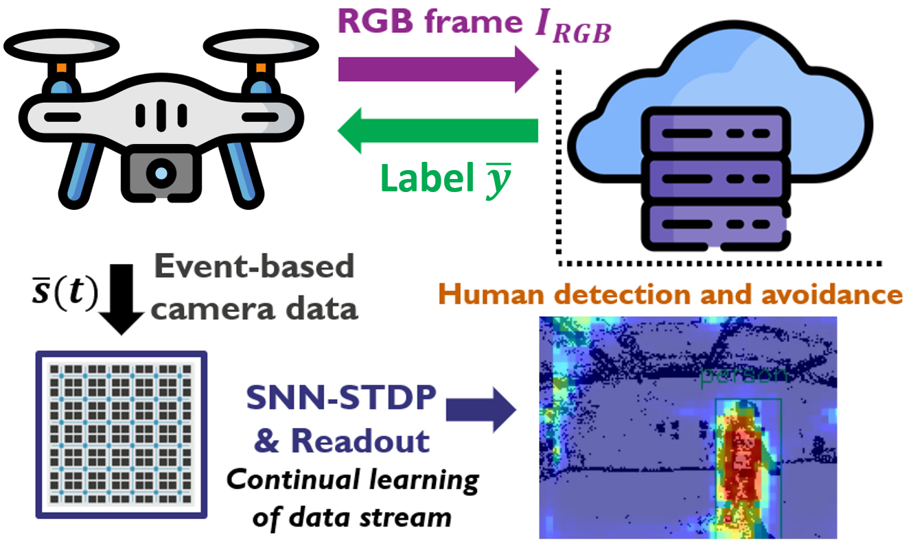
Indeed, conventional CNNs rely on the standard off-line training procedure where the CNN is trained on a large dataset capturing the task that needs to be solved. However, it is not always guaranteed that all scenarios to be encountered at run time are well captured by the training set (e.g., partially damaged infrastructures are hard to capture by a dedicated dataset for indoor search and rescue tasks). In addition, since CNN training requires desktop-grade computing, the conventional solution for fine-tuning on-board CNNs is to first re-train the network offline and then send the updated weights back to the drone. Clearly, this conventional approach has many drawbacks such as high latency (training takes a long time, prohibiting fast adaptation) and privacy concerns due to the on-line storage of user data (also causing legal issues due to e.g., the right to data erasure in the EU11 1 https://gdpr.eu/right-to-be-forgotten/).
Recently, the use of biologically-inspired spiking neural networks (SNNs) has gained huge interest for the design of ultra-low-power AI-enabled systems [12, 6]. In contrast to CNNs, SNNs make use of spiking neurons that communicate through low-complexity binary activations in an event-based manner (vs. frame-based processing in CNNs), only consuming energy when a spike is emitted [12]. In addition, SNNs can be implemented in massively parallel, non Von Neumann computing architectures, solving the energy- and latency-expensive memory bottleneck issues [6]. Finally, the use of a bio-inspired learning rule (vs. backprop) working in the binary activation domain and local to each neuron (such as Spike-Timing-Dependent Plasticity or STDP [8]) enables ultra-low-power learning at the edge (not tackled by embedded CNNs) [9]. Therefore, a growing number of SNN-STDP computing units have been proposed, achieving a power consumption as low as 0W [9] while enabling on-chip inference and learning (three orders of magnitude lower power consumption vs. optimized CNNs running on MCU [4]).
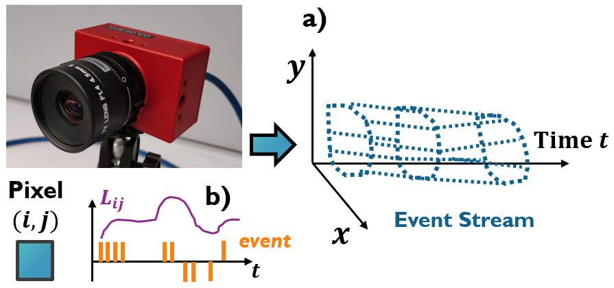
As SNNs require spiking data as input, they are often used in conjunction with an event-based camera (also called dynamic vision sensor or DVS), inspired by the inner working of the human eye. DVS cameras are composed of independent pixels that emit spikes asynchronously whenever the change in light log-intensity crosses a threshold [10] (see Fig. 1).
In this paper, our goal is to investigate the design of a bio-inspired SNN-STDP system that can continuously learn to perform people detection on drones from DVS camera data. Fig. 2 illustrates the scenario that we consider in this work: the drone must explore the environment during minutes and continuously learn to detect a walking human subject using the current data sample only, without access to the past and the future data. Then, continual learning (CL) is stopped and we assess the detection performance on a testing sequence.
As the basis for our people detection network, we use the state-of-the-art SNN-STDP architecture proposed in [12] and we augment it with three significant enhancements: i) we motivate and extend the SNN-STDP network to the use of anti-Hebbian (negative STDP) learning rules; ii) we propose a semi-supervised method that allows the learning of the logistic regression readout and the SNN at the same time (vs. disjoint learning in [12]) and iii) we use our SNN in a more challenging CL setting (vs. offline training in [12]).
This paper is organized as follows. Related works are discussed in Section II. Background theory is given in Section III. Our methods are presented in Section IV. Results are discussed in Section V. Conclusions are given in Section VI.

II Related Works
A growing number of bio-inspired robotic systems have been proposed in the past decades, mainly focusing on the study of animal-like actuation and motor control [11]. Complementary to bio-actuation, a number of perception systems for drones, taking inspiration from the inner workings of the human eye and the visual cortex, have recently emerged thanks to the advent of neuromorphic event-based cameras [6, 7, 10]. A line tracking system for drones was proposed in [6] using a DVS camera processed by an SNN. Similar to our work, the system of [6] uses an SNN with local bio-inspired learning rules (analogous to STDP) and demonstrates that such adaptive SNN system can learn to compensate for external disturbances online. Closer to our work, a DVS-based moving object tracking system for drones was proposed in [7], using hand-crafted feature extraction followed by Kalman filtering (processing pipeline not bio-plausible). Compared to the hand-crafted feature extraction in [7], we proposed a bio-inspired vision system that can continuously learn to detect walking people from a drone (vs. detecting any moving object in [7]).
Since sparsely-supervised and unsupervised learning are believed to be key mechanisms in the brain, a number of bio-inspired architectures have been proposed for learning spatio-temporal features from event-based data [18, 12]. Among them, the hierarchy of event-based time surfaces (HOTS) was proposed in [18] by cascading unsupervised layers, trained to cluster event-data aggregated as time surfaces (exponential decay maps) and by using an output readout (e.g., logistic regression) to classify the extracted features. In contrast to HOTS, which uses conventional clustering methods, an unsupervised SNN-STDP network with better biological plausibility was proposed by us in [12] for DVS feature learning, achieving state-of-the-art performance on common DVS benchmarks. Thus, we use the network of [12] as our basis in this work.
III Background theory
III-A SNN-STDP fundamentals
In contrast to CNNs, SNNs make use of spiking neurons, often modelled by a Leaky Integrate-and-Fire (LIF) activation:
| (1) |
with the input current to the neuron, the spiking output, the membrane potential, the membrane time constant and the neuron threshold [12]. The scalar input current is continuously integrated in following (1). When crosses the firing threshold , the membrane potential is reset back to zero and an output spike is emitted. The input current is obtained by filtering the inner product of the neural weights and the spiking inputs through a post-synaptic current (PSC) kernel [12] (estimating the spiking rate):
| (2) |
with the input spiking vector (originating from e.g. an event camera or other spiking neurons), the weight vector and the effect of PSC filtering with time constant . Fig. 3 a) conceptually illustrates the LIF neuron behaviour.
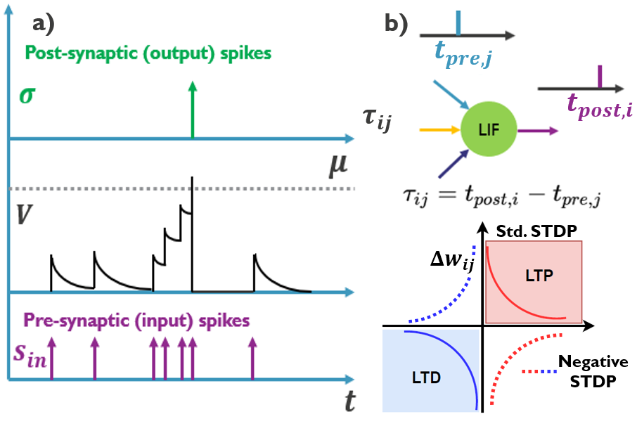
In the SNN architecture used in this work, learning is performed using the STDP rule, locally modifying the weights of each neuron as follows:
| (3) |
with the long-term potentiation (LTP) and depression (LTD) weights, the potentiation and depression decay constants, the element of the neuron weight vector and the time difference between the post- and the pre-synaptic spike times across the synapse of neuron (see Fig. 3 b) [8]. Finally, it can be shown [12] that a good approximation for the long-term effect of STDP (i.e., its expected value over time ) is given by the product of the post- and pre-synaptic mean spike rates (noted ):
| (4) |
where is the learning rate.
III-B SNN-STDP as Dictionary Learning, Basis Pursuit (DLBP)
As proposed in [12], the SNN-STDP in Fig. 4 is iteratively solving the unsupervised DLBP problem (inferring using the current and learning the next using the current ):
| (5) |
where is the -dimensional output vector containing the mean spike rates of each output neuron in the SNN, is the learned network weight matrix, is the -dimensional input vector, is a sparsity-controlling hyper-parameter and is a weight decay hyper-parameter.
DLBP (5) is solved iteratively by applying STDP across all neurons as follows [12]. The neuron in the error layer (see Fig. 4 b) receives as input the spike trains from the coding layer and outputs the reconstruction error in the spike domain:
| (6) |
where is locally modified by applying STDP with the as the post- and as the pre-synaptic spike trains. denotes the application of a push-pull pair of LIF neurons (1) (see Fig. 4 c). The neuron in the coding layer (see Fig. 4 a) receives and the previous output vector as input, and generates the output (where are the matrix rows):
| (7) |
with the output convergence rate (to be set) and the identity matrix of dimension . Each coding neuron also receives the error vector from the error layer and locally combines it with its inputs and to form the local signal :
| (8) |
Then, STDP is applied across each neuron using as the post- and as the pre-synaptic spike trains for learning . STDP is also applied using as the post- and as the pre-synaptic spike trains for learning [12]. Finally, it can be remarked that the SNN-STDP architecture of Fig. 4 can naturally be extended to the convolutional setting by sweeping the network of Fig. 4 across a image plane with kernel size and stride [12]. A spiking tensor of dimension:
| (9) |
is obtained. In this convolutional case, (5) can keep a similar form by considering as a circulant matrix and , , as flattened tensors along the image plane dimension.
IV Proposed methods
IV-A Extension to anti-Hebbian learning
Anti-Hebbian learning (or negative STDP, see Fig. 3 b) refers to the application of the opposite of the STDP rule (3) with negative and quantities in (3), and has been investigated in a few works [13]. Following the derivations in [12], it can be shown that using negative STDP for learning the input weights and feedback weights (see Fig. 4), while using standard STDP for the learning of the lateral weights (7), the following joint optimisation objective is solved:
| (10) |
Similar to (5), the SNN iterations infer the next SNN output by considering the current constant and learns the next SNN weight matrix by considering the current fixed.
Negative STDP solves (10) since:
| (11) |
and since it has been shown in [12] that standard STDP approximates the gradient-based learning:
| (12) |
it is now clear that negative STDP approximating:
| (13) |
is using a gradient similar to (11) (up to a dividing scalar oscillating around during our experiments) and is learning in (10). When combined with a supervision term (see Section IV-C), the use of the negative STDP rule can be motivated as a regularization controlling the over-fitting of the SNN-STDP by preventing the re-projection from becoming too small (see experiments in Section V-B).
IV-B Proposed bio-inspired SNN-STDP architecture
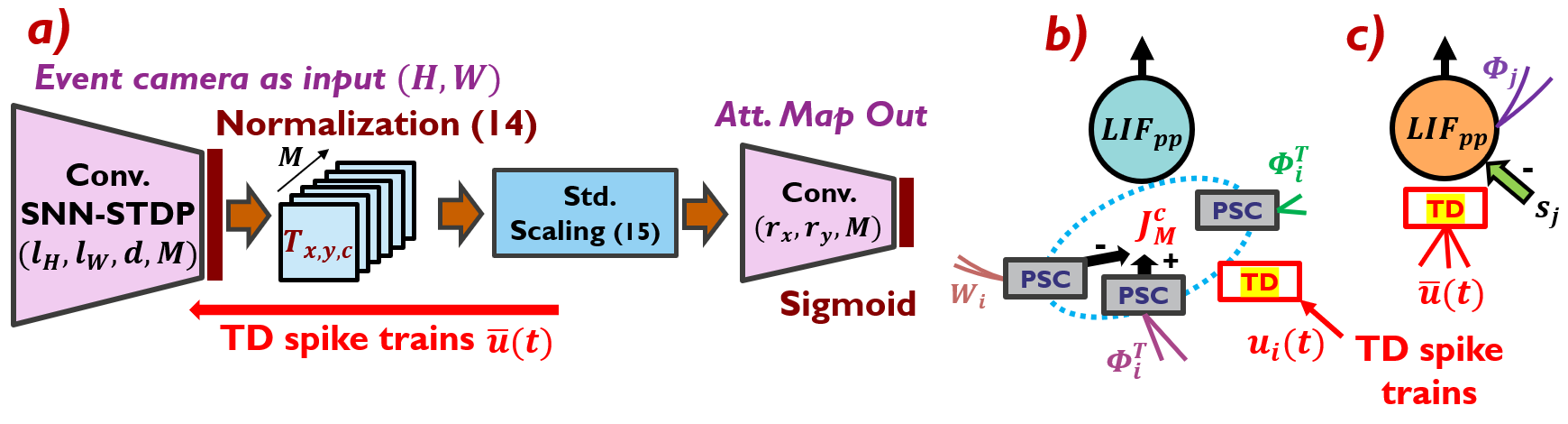
Fig. 5 a) shows the CL SNN-STDP system used throughout this work to infer attention maps. We set up a convolutional network by cascading the SNN-STDP network of Section IV-A (in a convolutional setting with negative STDP learning) with a convolutional readout in order to learn attention maps. At the output of the convolutional readout, we use sigmoid activation functions in order to constrain the dynamic range of the attention map between and . The rate of the spiking activity at the SNN output is estimated using a rolling time window of length . Doing so, a tensor containing the mean spike rates for each spatial coordinate and each channel is obtained. Then, is normalized along the channel dimension to provide invariance to event density [12]:
| (14) |
In between the SNN-STDP layer and the readout, we use standard scaling along the channel dimension in order to reduce the internal covariate shifts [14]:
| (15) |
where the mean and standard deviation are estimated on-line. We note the transformations (14)(15) of into as . Finally, is zero-padded and fed to the readout layer with a convolutional kernel size in order to obtain an attention map of dimension following (9). Finally, we interpolate the attention map back to the input size .
Without the use of the normalization mechanisms (14)(15), we observed the CL process to fail due to the severe covariate shifts encountered during learning. In addition, we observed that using a convolutional readout layer over a standard fully-connected layer is crucial in order to avoid readout overfitting on the local context encountered by the drone during the CL process (CL fails when using a fully-connected layer). The architecture of Fig. 5 a) also shows that the readout generates a vector of task-driven (TD) spike trains that is fed back to the SNN neurons. The TD spike trains are used to steer the unsupervised STDP-driven weight dynamics in order to jointly optimize the SNN weights and the readout , forming a task-driven, semi-supervised learning system.
IV-C Task-driven semi-supervised learning
During our experiments, we observe that the SNN-STDP system and the readout should not be optimised independently as in [12] (i.e., unsupervised learning of SNN and disjoint learning of a readout). Rather, the SNN and the readout must be learned concurrently. Indeed, if the learning process would be independent, the way the readout should fit the SNN output in the beginning of the STDP learning process will not be the same as in the end, since the SNN weights have independently changed since then, leading to significant covariate shifts at the input of the readout. Following this discussion, and the effectiveness of unsupervised DVS learning [12], we opt for a joint semi-supervised SNN-readout objective:
| (16) |
where in addition to (10), is the weight matrix of the readout, the learned bias vector, the sigmoid activation, the desired output label vector of dimension , the supervised loss function and the hyper-parameters controlling the strength of the unsupervised and supervised contributions. As usual, the network infers the next keeping constant, then learn keeping constant and so on. We choose as the focal loss because of its robustness to imbalanced data compared to the standard cross-entropy [15]:
| (17) |
with setting the robustness to class imbalance and:
| (18) |
In order to optimise as a function of the SNN weights , the link between and must be made explicit. Since is the result of an iterative process involving the LIF neuron non-linearity, an analytical function is hard to find and further relaxations must be done. First, we observe in (16) that for a small , is well approximated as:
| (19) |
Since is initialized following an i.i.d. zero-mean normal distribution with standard deviation [12], the following relaxation holds during the early SNN-STDP learning steps (when most of the learning effect takes place):
| (20) |
IV-D Task-driven SNN-STDP topology
Thanks to the relaxation (20)(21), the original unsupervised SNN-STDP architecture of Fig. 4 can now be modified in order to incorporate the effect of the newly added task-driven term in (16). We observe in (21) that:
| (22) |
is a vector computed at the readout side (e.g., in an MCU used to post-process the SNN activity) while the spike train vector in (21) is already available in both the coding and error layers (see Fig. 4 a). Therefore, the TD contribution can be injected in the SNN-STDP system by first converting to a push-pull pair of spike trains as follows:
| (23) |
Then, each entry of can be fed to the neuron in the coding layer via one additional synapse (see Fig. 5 b), and the spiking vector can be distributed to each error neuron via an additional set of synapses (see Fig. 5 c).
Finally, in addition to the unsupervised STDP mechanisms already present in the network of Fig. 4 to solve (5), it follows from (4) that an additional STDP contribution must be applied to the neurons in the error layer as follows:
| (24) |
with the post- and the pre-synaptic spike trains. An additional STDP contribution must also be applied to the neurons in the coding layer as:
| (25) |
with the post- and the pre-synaptic spike trains. Regarding the lateral weights , it can be shown [12] that the STDP mechanism adopted in the network of Fig. 4 automatically enforces consistency between the task-driven learning of and the convergence of (since applying STDP between in (8) and in (6) forces to converge to in (7) [12]).
IV-E Continual learning strategy
For on-line labelling, we use a pre-trained YOLOv3 network [5] to detect the presence or absence of a human subject from the RGB frames that are jointly acquired with the DVS data, and to infer the bounding box coordinates (normalized to the size of the output map) indicating the location of the human subject in the image. When a human subject is present, the corresponding label map (used for the supervised contribution) is assigned with ones inside the bounding box region and zeros outside. Since there are significantly more zero-valued entries in , we use median frequency balancing [16] to help mitigate the learning imbalance in space. Therefore, we weight the readout loss as follows:
| (26) |
where is the number of entries in of the same class as the label entry (the class can be either or in our detection case) and is the mean of and .
When no human subjects are detected, the label map will only contain null values for long iteration periods, leading to the over-fitting of the system on this local context. We alleviate this problem by keeping fixed when no human subjects are present, and only enabling learning for . In addition, we prune the task-driven contribution to the learning of (22) for values of smaller than a threshold (empirically found to work well). Doing so, we avoid the over-fitting of the system by sporadically learning hard examples only.
Regarding the choice of the on-line optimizer for the convolutional readout, we choose the Adam optimizer [17] because of its adaptive gradient scaling capability, which, in an on-line learning setting, leads to faster convergence compared to SGD. In addition, the use of momentum in Adam implicitly incorporates gradients from the data in hind-side, re-balancing the learning process over time [17].
IV-F Post-processing
A set of discrete detections is obtained from the attention map as follows. First, a threshold is applied to the map and a point cloud is formed. Then, a set of detected clusters is obtained by applying DBSCAN clustering [19] with min points and (empirically tuned).
V Experimental results
In this section, we assess the bio-inspired CL architecture described in Section IV on the KUL-UAVSAFE dataset [2] for people detection on drones. The KUL-UAVSAFE dataset features a collection of joint DVS and RGB acquisitions in an indoor, industrial-like environment, where a human subject is walking randomly. During our experiments, we choose the three longest acquisitions ( min.) from the f-wall collection in [2], where the drone and a human subject are moving in a space surrounded by walls, benches and shelves (different human subjects are featured to add variability).
We assess the performance of our system via 3-fold cross-validation as follows. First, one of the acquisitions is used as a learning sequence and is shown to our CL system only once, in its natural order (the learning sequence is not shuffled). Then, learning is stopped and a different acquisition is used to measure the precision-recall curves after post-processing (Section IV-F), by sweeping from to and measuring the number of false alarms, true positives and false negatives in . This process is repeated three times using different learning and testing sets and the final precision-recall curves are obtained as the average over the three learn-test folds.
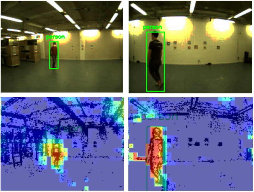
Fig. 6 shows examples of attention maps produced by our system. Table I reports the SNN-STDP learning parameters (found empirically, starting from the parameter set used in [12]). Table II reports the parameters used in our system architecture (tuned empirically). For the readout, we use the default values of the Adam optimizer [17] with a learning rate . Next, we will study the effect of the most important parameters impacting the CL procedure: the focal loss parameter (17) and the semi-supervision hyper-parameters (16).
| 1 | 0.8 | 0.02 | 0.008 | 0.01 |
|---|
| 130 | 173 | 30 | 5 | 64 | 12 | 21 | 29 |
V-A Impact of the focal loss parameter
We explore the impact of in (17) by keeping all other parameters constant with , . Fig. 7 shows the measured precision-recall curves. Fig. 7 also reports the peak score as along each precision-recall curve [2]. Fig. 7 shows that the peak score is maximised near . Therefore, in our experiments below.

V-B Impact of the unsupervised and supervised strengths
Fig. 8 shows the precision-recall curves obtained by varying the unsupervised (negative STDP) and supervised contributions in (16). Fig. 8 shows that the peak score is maximised near , .

During our experiments, we also tried the use of the standard positive STDP rule for the unsupervised contribution, but always reached lower performances by varying , due to an increase in false alarms. In contrast, the use of the negative STDP rule for the unsupervised contribution provides an opposite weight-steering force to the positive STDP rule used for the supervised contribution, preventing the over-fitting of the system to structures in the environment. This leads to less false alarms at higher recalls and therefore, a higher detection performance (a non-trivial gain of + on the peak score vs. , ).
V-C Continual SNN-STDP vs. standard CNNs
Since CNNs constitute the standard approach used in the vision pipelines of drones [4], we compare in Fig. 9 the performance of our CL architecture to two offline-trained CNNs: a SqueezeNet-based CNN trained with RGB data and a second SqueezeNet trained with DVS frames following [2] (DVS data averaged over time into frames at 30 FPS).

Using a SqueezeNet CNN architecture is an appropriate choice for comparison since SqueezeNet aims to be MCU-friendly, using KB of weight memory (comparable to our network that uses KB). In order to fairly compare the bounding box output of the CNN to the attention map of our SNN-STDP system, we consider the image region delimited by the bounding box as the active region of an attention map (region inside the bounding box is filled with and outside is filled with ). We can then use the same precision-recall measurement pipeline as used for the SNN. Fig. 9 shows that the CNN-RGB setup is the best performer (due to less false alarms compared to our SNN), but this comes at the cost of on-line adaptability. Indeed, the CNN has been trained offline for a specific environment and needs re-training each time new situations are encountered. This is in contrast to our CL SNN-STDP system which can learn and adapt on the fly, as demonstrated in this work. Interestingly, the CNN-DVS setup is the lowest performer and is significantly outperformed by the CL SNN-STDP system (+19% on the peak score). This is mainly due to the fact that the SNN introduces time recurrence through its lateral weights, enabling the network to learn temporal features that are neglected by the feed-forward CNN-DVS (see [18] for a discussion on temporal features in DVS data). This clearly shows the effectiveness of the methods proposed in Section IV for the continual learning of DVS data.
VI Conclusion
This paper has presented, to the best of our knowledge, the first continual learning system for drones that learns to detect people on the fly using a bio-inspired SNN architecture with STDP learning. After the introduction of our novel methods, numerous experiments have been described to characterize the performance of our system and compare it against conventional CNNs. We have shown that our event-based system reaches a higher peak score (+19%) compared to a same-size CNN processing DVS frames, while enabling on-line adaptation and learning on the fly. As future work, we plan to increase the precision of the system at higher recalls by studying how to enhance the SNN expressivity with more layers and reducing false alarms. We hope that this work will inspire future research in brain-inspired vision for robotics.
Acknowledgment
We thank Lars Keuninckx and Tim Verbelen for their precious help. The research leading to these results has received funding from the Flemish Government (AI Research Program) and the European Union’s ECSEL Joint Undertaking under grant agreement n° 826655 - project TEMPO.
References
- [1] D. Falanga, K. Kleber, S. Mintchev, D. Floreano and D. Scaramuzza, ”The Foldable Drone: A Morphing Quadrotor That Can Squeeze and Fly,” in IEEE Robotics and Automation Letters, vol. 4, no. 2, pp. 209-216, April 2019, doi: 10.1109/LRA.2018.2885575.
- [2] A. Safa, T. Verbelen, I. Ocket, A. Bourdoux, F. Catthoor and G. G. E. Gielen, ”Fail-Safe Human Detection for Drones Using a Multi-Modal Curriculum Learning Approach,” in IEEE Robotics and Automation Letters, vol. 7, no. 1, pp. 303-310, Jan. 2022, doi: 10.1109/LRA.2021.3125450.
- [3] W. Fang, L. Wang and P. Ren, ”Tinier-YOLO: A Real-Time Object Detection Method for Constrained Environments,” in IEEE Access, vol. 8, pp. 1935-1944, 2020, doi: 10.1109/ACCESS.2019.2961959.
- [4] D. Palossi, A. Loquercio, F. Conti, E. Flamand, D. Scaramuzza and L. Benini, ”A 64-mW DNN-Based Visual Navigation Engine for Autonomous Nano-Drones,” in IEEE Internet of Things Journal, vol. 6, no. 5, pp. 8357-8371, Oct. 2019, doi: 10.1109/JIOT.2019.2917066.
- [5] J. Redmon, A. Farhadi. (2018). ”YOLOv3: An Incremental Improvement.”
- [6] A. Vitale, A. Renner, C. Nauer, D. Scaramuzza and Y. Sandamirskaya, ”Event-driven Vision and Control for UAVs on a Neuromorphic Chip,” 2021 IEEE International Conference on Robotics and Automation (ICRA), 2021, pp. 103-109, doi: 10.1109/ICRA48506.2021.9560881.
- [7] A. Mitrokhin, C. Fermüller, C. Parameshwara and Y. Aloimonos, ”Event-Based Moving Object Detection and Tracking,” 2018 IEEE/RSJ International Conference on Intelligent Robots and Systems (IROS), 2018, pp. 1-9, doi: 10.1109/IROS.2018.8593805.
- [8] Bi, G.q., Poo, M.m. (1998). Synaptic Modifications in Cultured Hippocampal Neurons: Dependence on Spike Timing, Synaptic Strength, and Postsynaptic Cell Type. Journal of Neuroscience, 18(24), 10464–10472.
- [9] C. Frenkel, M. Lefebvre, J. -D. Legat and D. Bol, ”A 0.086-mm2 12.7-pJ/SOP 64k-Synapse 256-Neuron Online-Learning Digital Spiking Neuromorphic Processor in 28-nm CMOS,” in IEEE Transactions on Biomedical Circuits and Systems, vol. 13, no. 1, pp. 145-158, Feb. 2019, doi: 10.1109/TBCAS.2018.2880425.
- [10] G. Gallego et al., ”Event-based Vision: A Survey,” in IEEE Transactions on Pattern Analysis and Machine Intelligence, doi: 10.1109/TPAMI.2020.3008413.
- [11] A. J. Ijspeert (2008). ”Central pattern generators for locomotion control in animals and robots: A review.” Neural Networks, 21(4), 642-653.
- [12] Ali Safa et al., (2021). ”Learning Event-based Spatio-Temporal Feature Descriptors via Local Synaptic Plasticity: A Biologically-Plausible Perspective of Computer Vision.” (https://arxiv.org/abs/2111.00791), Submitted to IEEE Transaction on Neural Networks and Learning Systems.
- [13] T. Hu, C. Pehlevan and D. B. Chklovskii, ”A Hebbian/Anti-Hebbian network for online sparse dictionary learning derived from symmetric matrix factorization,” 2014 48th Asilomar Conference on Signals, Systems and Computers, 2014, pp. 613-619, doi: 10.1109/ACSSC.2014.7094519.
- [14] Ioffe, S. et al., (2015). ”Batch Normalization: Accelerating Deep Network Training by Reducing Internal Covariate Shift.” In Proceedings of the 32nd International Conference on Machine Learning (pp. 448–456).
- [15] T. -Y. Lin, P. Goyal, R. Girshick, K. He and P. Dollár, ”Focal Loss for Dense Object Detection,” in IEEE Transactions on Pattern Analysis and Machine Intelligence, vol. 42, no. 2, pp. 318-327, 1 Feb. 2020, doi: 10.1109/TPAMI.2018.2858826.
- [16] D. Eigen and R. Fergus, ”Predicting Depth, Surface Normals and Semantic Labels with a Common Multi-scale Convolutional Architecture,” 2015 IEEE International Conference on Computer Vision (ICCV), 2015, pp. 2650-2658, doi: 10.1109/ICCV.2015.304.
- [17] Diederik P. Kingma, Jimmy Ba. (2017). ”Adam: A Method for Stochastic Optimization.”
- [18] X. Lagorce, G. Orchard, F. Galluppi, B. E. Shi and R. B. Benosman, ”HOTS: A Hierarchy of Event-Based Time-Surfaces for Pattern Recognition,” in IEEE Transactions on Pattern Analysis and Machine Intelligence, vol. 39, no. 7, pp. 1346-1359, 1 July 2017, doi: 10.1109/TPAMI.2016.2574707.
- [19] Ester, M., Kriegel, H.P., Sander, J., Xu, X. (1996). ”A Density-Based Algorithm for Discovering Clusters in Large Spatial Databases with Noise.” In Proceedings of the Second International Conference on Knowledge Discovery and Data Mining (pp. 226–231). AAAI Press.