GAN Estimation of Lipschitz Optimal Transport Maps

Alberto González-Sanz Affiliation: Institut de Mathématiques de Toulouse, Université Paul Sabatier Lucas De Lara Affiliation: Institut de Mathématiques de Toulouse, Université Paul Sabatier Louis Béthune Affiliation: Institut de Recherche en Informatique de Toulouse, Université Paul Sabatier Jean-Michel Loubes Affiliation: Institut de Mathématiques de Toulouse, Université Paul Sabatier

Abstract

This paper introduces the first statistically consistent estimator of the optimal transport map between two probability distributions, based on neural networks. Building on theoretical and practical advances in the field of Lipschitz neural networks, we define a Lipschitz-constrained generative adversarial network penalized by the quadratic transportation cost. Then, we demonstrate that, under regularity assumptions, the obtained generator converges uniformly to the optimal transport map as the sample size increases to infinity. Furthermore, we show through a number of numerical experiments that the learnt mapping has promising performances. In contrast to previous work tackling either statistical guarantees or practicality, we provide an expressive and feasible estimator which paves way for optimal transport applications where the asymptotic behaviour must be certified.

1 Introduction

An optimal transport map is the fundamental object of Monge’s seminal formulation of optimal transport (Monge 1781). It transforms one distribution into another with minimal effort. Formally, given two probability distributions $P$ and $Q$ on $\Omega\subseteq\mathbb{R}^{d}$ , an optimal transport map from $P$ to $Q$ is a solution to,

\min_{T\in\mathcal{T}(P,Q)}\int_{\Omega}{\left\lVert x-T(x)\right\rVert}^{2}\mathrm{d}P(x),

(1)

where $\mathcal{T}(P,Q)$ is the set of measurable maps $T:\Omega\to\Omega$ pushing forward $P$ to $Q$ , that is $Q(M)=P(T^{-1}(M))$ for every measurable set $M\subseteq\Omega$ . This property, denoted by $T_{\sharp}P=Q$ , means that if a random variable $X$ follows the distribution $P$ then its image $T(X)$ follows the distribution $Q$ . According to Theorem 2.12 in (Villani 2003), originally demonstrated in (Cuesta and Matrán 1989; Brenier 1991), when $P$ and $Q$ admit densities with respect to the Lebesgue measure and have finite second-order moments, then there exists a unique (up to $P$ -negligible sets) solution to Problem (1), which we denote by $T_{0}$ .

Due to their transparent mathematical formulation and well-established theory, optimal transport maps became popular in many applications from statistics-related fields, where one aims at modeling shifts between distributions. This includes multivariate-quantile analysis (Beirlant et al. 2020; Hallin et al. 2021), signal analysis (Kolouri et al. 2017), domain adaptation (Courty et al. 2014; Seguy et al. 2018; Redko et al. 2019), transfer learning Gayraud et al. 2017, fairness in machine learning (Gordaliza et al. 2019; Black et al. 2020), and counterfactual reasoning (De Lara et al. 2021; Berk et al. 2021). However, in such practical frameworks, one typically does not have access to the true distributions $P$ and $Q$ but to independent samples $x_{1},\ldots,x_{n}\sim P$ and $y_{1},\ldots,y_{n}\sim Q$ . This raises the question of constructing a tractable approximation of the solution $T_{0}$ on the basis of these empirical observations. The simplest way to compute an empirical optimal transport map from data points is to solve Problem (1) between the empirical measures $P_{n}:=n^{-1}\sum^{n}_{i=1}\delta_{x_{i}}$ and $Q_{n}:=n^{-1}\sum^{n}_{i=1}\delta_{y_{i}}$ instead of $P$ and $Q$ . Implementing this solution suffers from three main drawbacks. The first one is the computational cost, since it requires at least $O(n^{3})$ operations to compute the empirical optimal transport map (Peyré and Cuturi 2019). The second is the memory cost, since this map is typically stored as an $n\times n$ matrix. As a consequence of these two issues, this approach does not scale well with the size of the dataset. The third limitation of the empirical map is its inability to generalize to new out-of-sample observations: by construction it is only matching the set $\{x_{1},\ldots,x_{n}\}$ to $\{y_{1},\ldots,y_{n}\}$ .

These practical drawbacks triggered a vast literature on continuous approximations of optimal transport maps. The proposed mappings all come with different practical limitations, theoretical guarantees, and experimental performances. On the one hand, a wide range of these constructions provably converge in some sense to the true map $T_{0}$ as $n$ increases to infinity, making them consistent estimators. The so-called plug-in estimators, such as the ones proposed in (Beirlant et al. 2020; Hallin et al. 2021; Manole et al. 2021), extend the empirical solution to the whole domain $\Omega$ by leveraging regularity assumptions. However, they still bear the burdens of computing and storing the empirical transport map. The smooth estimator introduced by Hütter and Rigollet 2021 reaches near-optimal minimax convergence rate, but fails to be computationally tractable. In contrast, Seguy et al. 2018 and Pooladian and Niles-Weed 2021 employed entropic regularization, a numerical scheme based on Sinkhorn’s algorithm (Cuturi 2013), to build an implementable and scalable estimator. On the other hand, several papers proposed learning the optimal transport map through neural networks, leading to expressive approximations with high generalization power. Specifically, Leygonie et al. 2019 and Black et al. 2020 developed approximations based on a generative-adversarial-network (GAN) objective (Goodfellow et al. 2014; Arjovsky et al. 2017). More recently, the use of input convex neural networks, building on the convexity of the optimal transport potential, has received a growing attention (Makkuva et al. 2020; Korotin et al. 2021; Huang et al. 2021). However, while these neural-based mappings display strong experimental performances, they generally lack theoretical guarantees, in particular the statistical convergence.

To sum-up, the literature has mostly addressed either theoretically grounded statistical estimators of optimal transport maps, but unsuitable for large-scale implementations, or efficient heuristic approximations, at the cost of statistical guarantees. In this paper, we propose a novel GAN-based estimator $G_{n}$ of $T_{0}$ which, under some assumptions, converges uniformly:

{\left\lVert G_{n}-T_{0}\right\rVert}_{\infty}\xrightarrow[n\to+\infty]{a.s.}0.

Our construction takes root in the approximation from (Black et al. 2020), defined as the generator of a penalized Wassertein-GAN (WGAN) training problem (Arjovsky et al. 2017), and improve it by assuming a setting where the optimal transport map is Lipschitz and by leveraging recent theoretical and practical advances on Lipschitz neural networks (Anil et al. 2019; Tanielian and Biau 2021; Béthune et al. 2021). Formally, $G_{n}$ solves the following adversarial training:

\inf_{G\in\mathcal{G}_{n}}\Big\{{\left\lVert I-G\right\rVert}^{2}_{L^{2}(P_{n})}+\lambda_{n}\sup_{D\in\mathcal{D}_{n}}\int D\left(\mathrm{d}(G_{\sharp}P_{n})-\mathrm{d}Q_{n}\right)\Big\},

where $\mathcal{D}_{n}$ is a class of 1-Lipschitz discriminators providing a proxy for the Wasserstein-1 distance, and $\mathcal{G}_{n}$ is a class of Lipschitz generators parametrizing the space of feasible mappings. The positive parameter $\lambda_{n}$ governs the trade-off between minimizing the quadratic transportation cost, promoting the objective of the Monge problem (1), and minimizing the distance between the generated and the target distributions, enforcing the push-forward constraint.

The most similar papers to ours are the ones of Seguy et al. 2018 and Pooladian and Niles-Weed 2021, as they propose feasible estimators with statistical guarantees. We note two main differences. First, we do not rely on entropic regularization while still ensuring scalability to large datasets. Second, our estimator innovates by being defined as a neural network. In particular, Seguy et al. 2018 relies on a neural network in practice, but the statistical convergence holds for a theoretical estimator. Regarding theoretical guarantees, we lack the convergences rates provided in (Pooladian and Niles-Weed 2021), but we prove a stronger result than Seguy et al. 2018 by ensuring the uniform convergence of the estimator.

Outline.

The rest of the paper is organized as follows:

1.

Section 2 introduces the necessary background on so-called GroupSort neural networks, which became the gold standard to parametrize Lipschiz feed-forward neural networks. By studying the multivariate setting, we provide generalizations of the main approximation theorem from (Tanielian and Biau 2021).
2.

Section 3 presents the technical assumptions of our framework, in particular the regularity of the optimal transport map, details construction of our GAN estimator, and states the statistical consistency theorem.
3.

Section 4 focuses on the practical implementation of the estimator, and study its performance through a number of numerical experiments.

Refer to caption — Figure 1: Estimation of the optimal transport map on the TwoMoons dataset. (a) GAN estimator $G$ after $800$ gradient steps on the generator, on the basis of $4,000$ points from each distribution. The black arrows represent the transport of specific points. (b) Empirical optimal transport map (discrete matching) between samples of size $500$ .

Notations.

The absolute value of real numbers and the Euclidean norm of vectors are respectively given by ${\left\lvert\cdot\right\rvert}$ and ${\left\lVert\cdot\right\rVert}$ . The notation $B_{r}$ refers to the centered Euclidean ball of $\mathbb{R}^{d}$ with radius $r>0$ . We denote by $\operatorname{diam}(\Omega)$ the diameter of a set $\Omega\subseteq\mathbb{R}^{d}$ . If $\Omega$ is a closed convex set, then $\mathcal{P}_{\Omega}$ stands for the projection onto $\Omega$ . The support of a probability measure is given by $\operatorname{supp}(\cdot)$ . In the following $\Omega_{1}\subseteq\mathbb{R}^{d_{1}}$ and $\Omega_{2}\subseteq\mathbb{R}^{d_{2}}$ denote two arbitrary subsets. For a function $F:\Omega_{1}\to\Omega_{2}$ and $\mu$ a probability measure on $\Omega_{1}$ , we write ${\left\lVert F\right\rVert}_{L^{2}(\mu)}:=\sqrt{\int_{\Omega_{1}}{\left\lVert F(x)\right\rVert}^{2}\mathrm{d}\mu(x)}$ . The supremum norm of function is given by ${\left\lVert\cdot\right\rVert}_{\infty}.$ For some $L>0$ , we write $\operatorname{Lip}_{L}(\Omega_{1},\Omega_{2})$ the set of $L$ -Lipschitz functions from $\Omega_{1}$ to $\Omega_{2}$ . For some $\alpha>0$ , we call $\mathcal{C}^{\alpha}(\Omega_{1},\Omega_{2})$ the set of $\alpha$ -Hölder functions from $\Omega_{1}$ to $\Omega_{2}$ and write ${\left\lVert\cdot\right\rVert}_{\alpha,\infty}$ for the $\alpha$ -Hölder norm of functions. For a differentiable function $F:\Omega_{1}\to\Omega_{2}$ , we call $F^{\prime}$ its derivative, where for any $x\in\Omega_{1}$ the quantity $F^{\prime}(x)$ is a $d_{1}\times d_{2}$ matrix. For a real symmetric matrix $S$ and a real number $\gamma$ , the relation $\gamma\preceq S$ indicates that all the eigenvalues of $S$ are greater than $\gamma$ . The relation $\succeq$ is defined similarly.

2 Lipschitz neural networks

The GAN estimator defined by (1) and further described in Section 3 requires generators and discriminators that are both Lipschitz. The question of imposing sharp Lipschitz constraints on neural networks has attracted much attention from the field of machine learning, especially with the popularization of WGANs which rely on 1-Lipschitz discriminators. In particular, gradient penalization (Gulrajani et al. 2017) has proven to be more efficient than the parameter-clipping approach originally proposed by Arjovsky et al. 2017. In this paper, we focus on the recently introduced GroupSort activation function to impose the Lipschitz constraint, which have proven to yield tighter estimates of 1-Lispchitz functions (Anil et al. 2019; Tanielian and Biau 2021). We recall the necessary background on GroupSort-based networks, and show that their ability to approximate any bounded classes of Lipschitz functions holds for arbitrary output dimension.

2.1 Multivariate GroupSort neural networks

We introduce GroupSort neural networks in a similar fashion to (Tanielian and Biau 2021). In contrast, we consider a more general setting where the output dimension $p\geq 1$ is arbitrary. This difference is motivated by the optimal transport map being a multivariate function.

We write $\sigma_{k}$ for the GroupSort activation function of grouping size $k\geq 2$ . By definition, it splits the pre-activation input into groups of size $k$ , and then sorts each group by decreasing order. This operation is 1-Lipschitz, gradient-norm preserving and homogeneous (Anil et al. 2019). In this paper, we only address the grouping size 2. We call a GroupSort feed-forward neural network (with grouping size 2) any function $N_{\theta}:\mathbb{R}^{d}\to\mathbb{R}^{p}$ of the form

N_{\theta}=h_{l}\circ h_{l-1}\circ\ldots\circ h_{1},

(2)

where

		$\displaystyle h_{1}(x):=W_{1}x+b_{1}\mbox{ with }W_{1}\in\mathbb{R}^{w_{1}\times d},b_{1}\in\mathbb{R}^{w_{1}};$
		$\displaystyle h_{2}(x):=W_{2}\sigma_{2}(x)+b_{2}\mbox{ with }W_{2}\in\mathbb{R}^{w_{2}\times w_{1}},b_{2}\in\mathbb{R}^{w_{2}};$
		$\displaystyle\ldots$
		$\displaystyle h_{l}(x):=W_{l}\sigma_{2}(x)+b_{l}\mbox{ with }W_{l}\in\mathbb{R}^{p\times w_{l-1}},b_{l}\in\mathbb{R}^{p}.$

The integer $l\geq 1$ denotes the depth of the network while the integers $\{w_{1},\ldots,w_{l-1}\}$ refer to the widths of the hidden layers $\{h_{1},\ldots,h_{l-1}\}$ . The widths are assumed to be divisible by $2$ (the grouping size). Additionally, we define $s:=\sum^{l-1}_{i=1}w_{i}$ the size of the network. The parameter $\theta:=(W_{1},\ldots,W_{l},b_{1},\ldots,b_{l})\in\Theta$ represents the weights matrices and offset vectors of $N_{\theta}$ .

For a matrix $W$ , let ${\left\lVert W\right\rVert}_{\infty}:=\sup_{{\left\lVert x\right\rVert}_{\infty}=1}{\left\lVert Wx\right\rVert}_{\infty}$ and ${\left\lVert W\right\rVert}_{2,\infty}:=\sup_{{\left\lVert x\right\rVert}=1}{\left\lVert Wx\right\rVert}_{\infty}$ , where ${\left\lVert x\right\rVert}_{\infty}$ denotes the maximum norm of vectors. Consider the following assumption on the parameters:

(C)

There exists a constant $C>0$ such that for all $(W_{1},\ldots,W_{l},b_{1},\ldots,b_{l})\in\Theta$ ,

	$\displaystyle{\left\lVert W_{1}\right\rVert}_{2,\infty}$	$\displaystyle\leq 1,$
	$\displaystyle\max({\left\lVert W_{2}\right\rVert}_{\infty},\ldots,{\left\lVert W_{l}\right\rVert}_{\infty})$	$\displaystyle\leq 1,$
	$\displaystyle\max({\left\lVert b_{1}\right\rVert}_{\infty},\ldots,{\left\lVert b_{l}\right\rVert}_{\infty})$	$\displaystyle\leq C.$

In the following, we denote by $\mathcal{N}^{p}_{C}(l,s)$ the class of GroupSort feed-forward neural networks with depth $l$ , size $s$ , output dimension $p$ , satisfying Assumption (C) for the constant $C>0$ . When the depth and size are arbitrary, we simply write $\mathcal{N}^{p}_{C}$ . The following result is a trivial extension to the multivariate case of Lemma 1 in (Tanielian and Biau 2021), stating that GroupSort neural networks satisfying Assumption (C) are 1-Lipschitz.

Lemma 2.1.

For any $C>0$ , $\mathcal{N}^{p}_{C}\subset\operatorname{Lip}_{1}(\mathbb{R}^{d},\mathbb{R}^{p})$ .

Next, we study their ability to approximate Lipschitz continuous functions.

2.2 Approximating Lipschitz continuous functions

We now restrict the input domain to a compact subset of $\mathbb{R}^{d}$ denoted by $\Omega$ . The following lemma states that for a well-chosen $C$ the class $\mathcal{N}^{1}_{C}$ approximates with given precision any bounded subclass of $\operatorname{Lip}_{1}(\Omega,\mathbb{R})$ . It generalizes Theorem 2 in (Tanielian and Biau 2021) by providing the universal constant for which Assumption (C) is satisfied, and extending the result to any compact domain $\Omega$ while it was restricted to $[0,1]^{d}$ .

Theorem 2.1.

Let $\mathcal{F}\subseteq\operatorname{Lip}_{1}(\Omega,\mathbb{R})$ be a class of functions such that $\sup_{f\in\mathcal{F}}{\left\lVert f\right\rVert}_{\infty}\leq K_{\mathcal{F}}$ for some $K_{\mathcal{F}}>0$ . Set $\epsilon>0$ and $C:=K_{\mathcal{F}}+\sqrt{d}(\sup_{x\in\Omega}{\left\lVert x\right\rVert}+1)+\epsilon$ . Then, for any $f\in\mathcal{F}$ , there exists a neural network $N\in\mathcal{N}^{1}_{C}(l,s)$ where

l=O\left(d^{2}\log_{2}\left(\frac{2\sqrt{d}}{\epsilon}\right)\right)\ \text{and}\ s=O\left(\left(\frac{2\sqrt{d}}{\epsilon}\right)^{d^{2}}\right),

such that ${\left\lVert N-f\right\rVert}_{\infty}\leq\epsilon$ .

The proof essentially follows that of Tanielian and Biau 2021. It generalizes some parts by tracking the bound on the offset vectors of the approximating network. Interestingly, Theorem 2.1 can be extended to the case where the output is of dimension $p$ .

Theorem 2.2.

Let $\mathcal{G}\subseteq\operatorname{Lip}_{1}(\Omega,\mathbb{R}^{p})$ be a class of functions such that $\sup_{g\in\mathcal{G}}{\left\lVert g\right\rVert}_{\infty}\leq K_{\mathcal{G}}$ for some $K_{\mathcal{G}}>0$ . Set $\varepsilon>0$ and $C=K_{\mathcal{G}}+\sqrt{d}(\sup_{x\in\Omega}{\left\lVert x\right\rVert}+1)+\varepsilon$ . Then, for any $g\in\mathcal{G}$ there exists a neural network $N\in\mathcal{N}^{p}_{C}(l,s)$ where

l=O\left(d^{2}\log_{2}\left(\frac{2\sqrt{d}\sqrt{p}}{\epsilon}\right)\right),\ \ \text{and}\ \ s=O\left(p\left(\frac{2\sqrt{d}\sqrt{p}}{\epsilon}\right)^{d^{2}}\right),

such that ${\left\lVert N-g\right\rVert}_{\infty}\leq\varepsilon$ .

The proof amounts to applying Theorem 2.1 to the univariate function along each dimension. Note that Theorems 2.1 and 2.2 can be extended to approximate $L$ -Lipschitz functions, for an arbitrary $L>0$ , by multiplicating by $L$ the output later of 1-Lipschitz neural networks. This remark will be useful to approximate the optimal transport map, assumed to be $L$ -Lipschitz.

3 GAN estimator

In this section, we address the construction of an estimator of the optimal transport map, and show its uniform convergence as the sample size increases to infinity.

3.1 Optimal transport setup

Set $P$ and $Q$ two measures on $\mathbb{R}^{d}$ admitting densities with respect to the Lebesgue measure and with finite second-order moments. We aim at estimating with a GroupSort neural network the unique optimal transport map $T_{0}$ between $P$ and $Q$ through the knowledge of the empirical distributions $P_{n}$ and $Q_{n}$ . As mentioned in the introduction, we consider a setting where the optimal transport map $T_{0}$ is Lipschitz.

As in the previous section, $\Omega\subset\mathbb{R}$ is a compact set, and we denote by $\Omega_{P}:=\operatorname{supp}(P)$ the source domain and $\Omega_{Q}:=\operatorname{supp}(Q)$ the target domain. Then, we let $L\geq 2$ and make the following assumptions:

(S1)

The source domain $\Omega_{P}\subseteq B_{L}$ is a bounded and connected Lipschitz domain. The measure $P$ admits a density $\rho$ with respect to the Lebesgue measure such that $L^{-1}\leq\rho(x)\leq L$ for almost every $x\in\Omega_{P}$ .

(S2)

Let $\tilde{\Omega}_{P}$ denote a convex set with Lipschitz boundary such that $\Omega_{P}+B_{L^{-1}}\subseteq\tilde{\Omega}_{P}\subseteq B_{L}$ . The optimal transport map $T_{0}$ is a differentiable function from $\tilde{\Omega}_{P}$ to $\mathbb{R}^{d}$ such that $T_{0}=\nabla f_{0}$ where $f_{0}:\tilde{\Omega}_{P}\to\mathbb{R}^{d}$ is a differentiable convex function. Additionally it satisfies:

(i)

$T_{0}\in C^{2}(\tilde{\Omega}_{P},\mathbb{R}^{d})$ such that ${\left\lVert T_{0}\right\rVert}_{2,\infty}\leq L$ ;
(ii)

$L^{-1}\preceq T^{\prime}_{0}(x)\preceq L$ for all $x\in\tilde{\Omega}_{P}$ .

These are the same hypothesis as in Section 5 from (Hütter and Rigollet 2021), specified with a Hölder regularity $\alpha$ equals to 2. This makes our setting milder, as we do not require the optimal transport map to be highly regular. Assumptions (S1) and (S2) ensure the existence of a near-optimal minimax estimator of $T_{0}$ , which play a key role in the proof of our estimator’s consistency. Note that, without loss of generality, we can consider that $P$ and $Q$ are measures on a compact set $\Omega\subset\mathbb{R}^{d}$ sufficiently large to contain $B_{L}$ . Then, Assumption (S2) implies that $T_{0}\in\operatorname{Lip}_{L}(\Omega,B_{L})$ .

Now that the optimal transport problem is properly specified, we turn to the GAN architecture through which our estimator is defined.

3.2 GAN setup

The optimal transport map $T_{0}$ satisfies two objectives: it is constrained to pushing-forward $P$ to $Q$ , that is ${T_{0}}_{\sharp}P=Q$ ; it minimizes the quadratic transportation cost ${\left\lVert I-T_{0}\right\rVert}^{2}_{L^{2}(P)}$ . Due to the push-forward condition, $T_{0}$ can be regarded as a generative model. This observation is the foundation of the approximation of Black et al. 2020. They proposed to regularize the WGAN objective function, promoting only the push-forward condition, with an optimal transport penalty on the generator. We proceed similarly, with three critical differences. First, we penalize the quadratic transportation cost with the push-forward condition instead of the converse. Second, we employ GroupSort neural networks to implement the discriminator and generator. Third, because we aim at proving the statistical convergence of the generator, we emphasize for all the objects involved in the GAN their dependence to the sample size $n$ , including the penalty weight.

3.2.1 Discriminator

In the WGAN framework, the discriminator $D:\mathbb{R}^{d}\to\mathbb{R}$ is a neural network defining a proxy for the Wasserstein-1 distance, while the generator $G:\mathbb{R}^{d}\to\mathbb{R}^{d}$ is a neural network minimizing this proxy between ${G}_{\sharp}P_{n}$ and $Q_{n}$ , thereby aiming at generating $Q$ from $P$ .

We recall that the Wasserstein-1 distance between two measures $\mu$ and $\nu$ on $\Omega$ is defined as,

\mathcal{W}(\mu,\nu):=\inf_{\pi\in\Pi(\mu,\nu)}\int_{\Omega\times\Omega}{\left\lVert x-y\right\rVert}\mathrm{d}\pi(x,y),

where $\Pi(\mu,\nu)$ is the set of couplings with $\mu$ as first marginal and $\nu$ as second marginal. Interestingly, this distance enjoys the following dual formulation, known as the Kantorovich-Rubinstein formula (Kantorovich and Rubinshtein 1958). According to the Particular Case 5.15 of Theorem 5.9 in (Villani 2008), this can be written as:

\mathcal{W}(\mu,\nu)=\sup_{f\in\operatorname{Lip}_{1}(\Omega,\mathbb{R})}\int f(\mathrm{d}\mu-\mathrm{d}\nu).

(3)

The key idea of WGAN is to approximate this distance by computing the supremum over a class of neural networks included in $\operatorname{Lip}_{1}(\Omega,\mathbb{R})$ . The larger the class, the better the approximation. Originally, this was done by clipping, thresholding the weights of the network, leading to a coarse approximation of the Wasserstein distance. Later, several papers showed that using GroupSort neural networks led to sharper approximations (Anil et al. 2019; Biau et al. 2021).

Actually, note that if $f$ is an optimal function in Problem (3), then the function $f+c$ for any constant $c$ is also an optimal solution. As a consequence, we can without loss of generality restrict the set of feasible potentials to 1-Lipschitz functions taking the value zero at a given arbitrary anchor point $x_{0}\in\Omega$ . Formally, let’s define

\mathcal{F}:=\{f\in\operatorname{Lip}_{1}(\Omega,\mathbb{R})\mid f(x_{0})=0\}.

(4)

Then we can write,

\mathcal{W}(\mu,\nu)=\sup_{f\in\mathcal{F}}\int f(\mathrm{d}\mu-\mathrm{d}\nu).

The interest of this formulation is that the feasible potentials now belongs to a bounded subclass of Lipschitz functions.

Lemma 3.1.

Let $\mathcal{F}$ be defined as in Equation (4). Then,

K_{\mathcal{F}}:=\sup_{f\in\mathcal{F}}{\left\lVert f\right\rVert}_{\infty}\leq\operatorname{diam}(\Omega).

Thus, Theorem 2.1 entails that they can be approximated by GroupSort neural networks with specific depth and size. Following this remark, we define for each sample size $n$ the class of feasible discriminators $\mathcal{D}_{n}$ as well-chosen GroupSort neural networks. Specifically, the discriminators are defined as in the next assumption.

(G1)

Set a sequence of positive numbers $\{\epsilon_{n}\}_{n\in\mathbb{N}}$ such that $\lim_{n\to+\infty}\epsilon_{n}=0$ , and a sequence of constants $\{C_{n}\}_{n\in\mathbb{N}}$ defined as

C_{n}:=\operatorname{diam}(\Omega)+\sqrt{d}(\sup_{x\in\Omega}{\left\lVert x\right\rVert}+1)+\epsilon_{n}.

For every $n\in\mathbb{N}$ , define $\mathcal{D}_{n}:=\mathcal{N}^{1}_{C_{n}}(l_{n},s_{n})$ where,

l_{n}=O\left(d^{2}\log_{2}\left(\frac{2\sqrt{d}}{\epsilon_{n}}\right)\right),\ \ \text{and}\ \ s_{n}=O\left(\left(\frac{2\sqrt{d}}{\epsilon_{n}}\right)^{d^{2}}\right).

Then, we approximate the Wasserstein-1 distance through the following integral probability metric:

\mathcal{W}_{n}(\mu,\nu):=\sup_{D\in\mathcal{D}_{n}}\int D(\mathrm{d}\mu-\mathrm{d}\nu).

(5)

An important consequence of Assumption (G1) through Lemma 3.1 and Theorem 2.1 is that $\bigcup_{n\in\mathbb{N}}\mathcal{D}_{n}$ is dense in $\mathcal{F}$ , rendering $\mathcal{W}_{n}$ asymptotically close to $\mathcal{W}$ as $n$ increases to infinity. Note that the sequence $\{\epsilon_{n}\}_{n\in\mathbb{N}}$ characterizes the rate at which the class $\mathcal{D}_{n}$ approximates $\mathcal{F}$ . Now that we have properly defined the discriminators, we focus on the generators.

3.2.2 Generator

On the contrary to a standard WGAN, the generator must additionally minimize the quadratic transportation cost in order to approach the optimal transport map $T_{0}$ . Let us denote by $\mathcal{G}_{n}$ the class of feasible generators, which will be specified later. A naive formulation for our estimator $G_{n}\in\mathcal{G}_{n}$ would be,

G_{n}\in\argmin_{G\in\mathcal{G}_{n}\text{ s.t. }{G}_{\sharp}P_{n}=Q_{n}}{\left\lVert I-G\right\rVert}^{2}_{L^{2}(P_{n})}.

However, since the push-forward condition is intractable as such, we replace it by a penalty term based on the neural proxy of the Wasserstein-1 distance. Formally, we set $\lambda_{n}>0$ a regularization weight and we define the GAN estimator $G_{n}$ as an optimal solution to Problem (1), that is

G_{n}\in\argmin_{G\in\mathcal{G}_{n}}\mathcal{L}_{n}(G),

where

\mathcal{L}_{n}(G):={\left\lVert I-G\right\rVert}^{2}_{L^{2}(P_{n})}+\lambda_{n}\mathcal{W}_{n}(G_{\sharp}P_{n},Q_{n}).

We note that Problem (1) is well-posed under mild conditions.

Proposition 3.1.

If $\mathcal{D}_{n}\subseteq\operatorname{Lip}_{1}(\Omega,\mathbb{R})$ and $\mathcal{G}_{n}$ is compact, then Problem (1) admits solutions.

This result is a direct consequence of the Lipschitz continuity of the loss function $\mathcal{L}_{n}$ , which we demonstrate in the proof.

At this stage, we should make further assumptions on $\mathcal{G}_{n}$ to exploit the smoothness of the optimal transport problem. Let us define

\mathcal{G}:=\operatorname{Lip}_{L}(\Omega,B_{L}),

(6)

which is a class of bounded Lipschitz functions.

Lemma 3.2.

Let $\mathcal{G}$ be defined as in Equation (6). Then,

K_{\mathcal{G}}:=\sup_{g\in\mathcal{G}}{\left\lVert g\right\rVert}_{\infty}\leq L\operatorname{diam}(\Omega)+\sup_{x\in\Omega}{\left\lVert x\right\rVert}.

Critically, under Assumption (S2), the solution $T_{0}$ belongs to $\mathcal{G}$ , and as such can be approximated by GroupSort neural networks according to Theorem 2.2. This motivates the following conditions on the set of feasible generators $\mathcal{G}_{n}$ :

(G2)

Set $\{\varepsilon_{n}\}_{n\in\mathbb{N}}$ a sequence of positive numbers such that $\lim_{n\to+\infty}\varepsilon_{n}=0$ , and a sequence of constants $\{C_{n}\}_{n\in\mathbb{N}}$ defined as

C_{n}:=L\operatorname{diam}(\Omega)+(\sqrt{d}+1)\sup_{x\in\Omega}{\left\lVert x\right\rVert}+\sqrt{d}+\varepsilon_{n}.

For every $n\in\mathbb{N}$ , we define $\mathcal{G}_{n}$ as

\{x\in\Omega\mapsto\mathcal{P}_{B_{L}}(L\times N(x)),N\in\mathcal{N}^{d}_{C_{n}}(l_{n},s_{n})\}

where,

l_{n}=O\left(d\log_{2}\left(\frac{2d}{\varepsilon_{n}}\right)\right),\ \ \text{and}\ \ s_{n}=O\left(d\left(\frac{2d}{\varepsilon_{n}}\right)^{d^{2}}\right).

Defined as such, $\mathcal{G}_{n}$ is included in $\mathcal{G}$ . The idea behind Assumption (G2) is similar to that of Assumption (G1). In particular, the condition on the depth and size of the networks guarantees through Theorem 2.2 that $\mathcal{G}_{n}$ asymptotically fills $\mathcal{G}$ at speed $\varepsilon_{n}$ , allowing to recover $T_{0}$ at the limit.

3.3 Main theorem

The convergence of $\{G_{n}\}_{n\in\mathbb{N}}$ towards $T_{0}$ revolves around two antagonistic conditions. Instinctively, the sequence of regularization weights $\{\lambda_{n}\}_{n\in\mathbb{N}}$ must tend to infinity in order to impose the push-forward condition at the limit. Concurrently, the sequence of feasible generators $\{\mathcal{G}_{n}\}_{n\in\mathbb{N}}$ must fill $\mathcal{G}$ sufficiently fast. This corresponds to the following assumptions:

(G3)

The sequence $\{\lambda_{n}\}$ is such that $\lim_{n\to+\infty}\lambda_{n}=+\infty$ and

\lambda_{n}=\begin{cases}o\left(n^{\frac{1}{d}}\right)&\mbox{if }d>2,\\ o\left(n^{\frac{1}{2}}/\log n\right)&\mbox{if }d=2,\\ o\left(n^{\frac{1}{2}}/\sqrt{\log n}\right)&\mbox{if }d=1.\\ \end{cases}

(G4)

The sequence $\{\varepsilon_{n}\}_{n\in\mathbb{N}}$ from Assumption (G2) is such that, $\varepsilon_{n}=o\left(\frac{1}{\lambda_{n}}\right)$ .

We are now ready to state our main theorem.

Theorem 3.1.

Let $P$ and $Q$ be such that the smoothness assumptions (S1) and (S2) on the optimal transport problem hold, and denote by $T_{0}$ the (almost everywhere) unique optimal transport map between $P$ and $Q$ . Suppose that the GAN problem satisfies Assumptions (G1), (G2), (G3) and (G4). Then, for $G_{n}$ defined as a solution to Problem (1) we have

{\left\lVert G_{n}-T_{0}\right\rVert}_{\infty}\xrightarrow[n\to+\infty]{a.s.}0.

To the best of our knowledge, this is the first statistical consistency result for a neural-network-based optimal transport map. We leave the analysis of consistency rates for future work. In particular, we could obtain sharper results by imposing conditions on the parameter $\epsilon_{n}$ which characterizes the rate at which the discriminators $\mathcal{D}_{n}$ approximate the 1-Lipschitz potentials, and by leveraging stronger regularity assumptions on $T_{0}$ . The proof is quite technical; the convergence of $\lambda_{n}$ to infinity prevents from using classical empirical process techniques. Instead, we rely on more analytical arguments based on the relative compactness properties of Lipschitz functions. Moreover, we note that the proof still holds for more general classes of generators as long as they maintain certain universality properties and have a Lipschitz constant that can be controlled. This is one of the main strengths of GroupSort neural networks: they can sharply approximate any classes of bounded Lipschitz functions with the same Lipschitz constant.

4 Numerical experiments

The rest of the paper addresses the implementation of our method, and showcases experimental results. Specifically, we do not try to illustrate the convergence rate of the estimator, which is yet to be found, but instead focus on the efficiency and practicality of our GAN-based optimal transport map.

4.1 Implementation

In the following experiments, we use ( $\cdot\rightarrow 80\rightarrow 80\rightarrow 80\rightarrow\cdot$ ) densely connected neural networks with GroupSort activation functions for both the generator and the discriminator. We implement GroupSort using Deel-Lip library¹¹ 1 https://deel-lip.readthedocs.io. The 1-Lipschitz constraint is enforced through projections onto a parameter space satisfying Assumption (C). The output layer of the generator is multiplied by $L$ to be made $L$ -Lipschitz. Critically, since this constant is unknown in practice, we must rely on a large-enough user-defined upper bound. We use Adam with default parameters for the optimization. All experiments have been run on personal workstation with 32GB RAM and NVIDIA Quadro RTX 8000 48GB GPU.

Algorithm 1 GAN learning of the optimal transport map

Input: source distribution

P

, target distribution

Q

, regularization parameter

\lambda

, discriminator

\{D_{\psi}\}_{\psi\in\Psi}

, generator

\{G_{\phi}\}_{\phi\in\Phi}

, respective learning rates

\eta_{D}

and

\eta_{G}

, minibatch size

m

repeat

Sample minibatchs:

\{x_{i}\}^{m}_{i=1}\sim P

\{y_{i}\}^{m}_{i=1}\sim Q

Define cost function:

\mathcal{W}_{D}(\psi)\mathrel{\mathop{:}}=\frac{1}{m}\sum^{m}_{i=1}D_{\psi}(G_{\phi}(x_{i}))-\frac{1}{m}\sum^{m}_{i=1}D_{\psi}(y_{i})

Projected gradient ascent step on discriminator:

\psi\leftarrow\mathcal{P}_{\Psi}\left(\psi+\eta_{D}\nabla_{\psi}\mathcal{W}_{D}(\psi)\right)

until convergence of

D_{\psi}

Sample minibatch:

\{x^{\prime}_{i}\}^{m}_{i=1}\sim P

Define cost functions:

\displaystyle\begin{aligned} \mathcal{W}_{G}(\phi)\mathrel{\mathop{:}}=&\frac{1}{m}\sum^{m}_{i=1}D_{\psi}(G_{\phi}(x^{\prime}_{i}))\\ \mathcal{C}(\phi)\mathrel{\mathop{:}}=&\frac{1}{m}\sum^{m}_{i=1}{\left\lVert x^{\prime}_{i}-G_{\phi}(x^{\prime}_{i})\right\rVert}^{2}\end{aligned}

Projected gradient descent step on generator:

\phi\leftarrow\mathcal{P}_{\Phi}\left(\phi-\eta_{G}\nabla_{\phi}(\mathcal{C}(\phi)+\lambda\mathcal{W}_{G}(\phi))\right)

until convergence of

G_{\phi}

The learning procedure is detailed in Algorithm 1. In contrast to a WGAN, the generator loss includes the quadratic transportation cost. It also differs from the procedure proposed in (Black et al. 2020) by implementing a sharper weight projection than clipping.

4.2 Experimental results

We evaluate how close the trained generator $G$ is to the optimal transport map $T_{0}$ . Recall that our construction, as in (Hütter and Rigollet 2021; Pooladian and Niles-Weed 2021), is tailored to settings where the optimal transport map is at least Lipschitz, hence continuous. This excludes in particular target distributions with disconnected supports. Firstly, we address a setting where the true optimal transport map $T_{0}$ in unknown. Figure 1 benchmarks the GAN estimator against the empirical optimal transport map on the TwoMoons dataset. We used the POT library to compute the discrete matching (Flamary et al. 2021). It shows that the generator faithfully matches the two moons with respect to the quadratic transportation cost.

Secondly, we consider synthetic examples for which $T_{0}$ has an explicit formula. We follow the protocol adopted in the aforementioned papers by defining $P$ as the uniform distribution on the hypercube $[-1,1]^{d}$ and setting $Q:={T_{0}}_{\sharp}P$ , where $T_{0}:\mathbb{R}^{d}\to\mathbb{R}^{d}$ is obtained by applying a monotone scalar function coordinate-wise. The combination of McCann’s theorem (McCann 1995), stating that there exists a unique gradient of a convex function achieving the push-forward between two Lebesgue-absolutely-continuous distributions, and Theorem 2.12 in (Villani 2003), stating that an optimal transport map coincide almost-everywhere with the gradient of a convex function, ensures that $T_{0}$ constructed as such is the (almost everywhere unique) optimal transport map between $P$ and $Q$ . Note that for practical reasons, we choose $T_{0}$ such that $Q$ is a distribution with zero mean and width less than $2$ : normalizing the input and output distributions of a neural network ensures faster convergence. The result are illustrated in Figure 2.

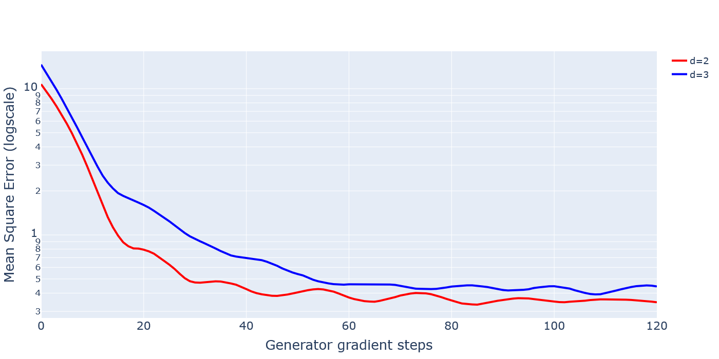
Additionally, we investigate in Figure 3 the evolution of the mean square error between the generator $G$ and the optimal transport map $T_{0}$ as the learning process goes on. It confirms that the optimization scheme has the expected behaviour. Furthermore, since the mean square error is evaluated on an independent sample to the training set, it illustrates the generalization ability of the learnt map.

5 Conclusion

The method we propose has the advantage of providing a theoretically sound and feasible estimation of the optimal transport map whose statistical convergence can be mathematically certified. Theorem 3.1 proves its consistency, while Section 4 highlights its feasibility and illustrates its ability to learn the underlying map. This renders this estimator suitable for many applications where guarantees of convergence are required while maintaining a high level of computational performance.

Additionally, we extended in Section 2 the established theory on approximating Lipschitz continuous functions by GroupSort neural networks to the multivariate case. This also opens new lines of inquiry for further applications of these networks, such as imposing regularity properties on generative models. Finally, our statistical framework and mathematical proofs addressed several interesting problems at the frontier between neural network modeling and statistics. We hope this effort will contribute to bridge the gap between deep learning and statistical theory.

References

Anil et al. (2019) C. Anil, J. Lucas, and R. Grosse. Sorting out Lipschitz function approximation. In International Conference on Machine Learning, pages 291–301. PMLR, 2019.
Arjovsky et al. (2017) M. Arjovsky, S. Chintala, and L. Bottou. Wasserstein generative adversarial networks. In International Conference on Machine Learning, pages 214–223. PMLR, 2017.
Beirlant et al. (2020) J. Beirlant, S. Buitendag, E. del Barrio, M. Hallin, and F. Kamper. Center-outward quantiles and the measurement of multivariate risk. Insurance: Mathematics and Economics, 95:79–100, 2020.
Berk et al. (2021) R. A. Berk, A. K. Kuchibhotla, and E. T. Tchetgen. Improving fairness in criminal justice algorithmic risk assessments using optimal transport and conformal prediction sets. arXiv preprint arXiv:2111.09211, 2021.
Biau et al. (2021) G. Biau, M. Sangnier, and U. Tanielian. Some theoretical insights into Wasserstein GANs. Journal of Machine Learning Research, 2021.
Black et al. (2020) E. Black, S. Yeom, and M. Fredrikson. Fliptest: fairness testing via optimal transport. In Conference on Fairness, Accountability, and Transparency, pages 111–121, 2020.
Boucheron et al. (2013) S. Boucheron, G. Lugosi, and P. Massart. Concentration inequalities: A nonasymptotic theory of independence. Oxford university press, 2013.
Brenier (1991) Y. Brenier. Polar factorization and monotone rearrangement of vector-valued functions. Communications on pure and applied mathematics, 44(4):375–417, 1991.
Béthune et al. (2021) L. Béthune, A. González-Sanz, F. Mamalet, and M. Serrurier. The many faces of 1-Lipschitz neural networks, 2021.
Courty et al. (2014) N. Courty, R. Flamary, and D. Tuia. Domain adaptation with regularized optimal transport. In Joint European Conference on Machine Learning and Knowledge Discovery in Databases, pages 274–289. Springer, 2014.
Cuesta and Matrán (1989) J. A. Cuesta and C. Matrán. Notes on the Wasserstein metric in Hilbert spaces. The Annals of Probability, pages 1264–1276, 1989.
Cuturi (2013) M. Cuturi. Sinkhorn distances: Lightspeed computation of optimal transport. Advances in neural information processing systems, 26:2292–2300, 2013.
De Lara et al. (2021) L. De Lara, A. González-Sanz, N. Asher, and J.-M. Loubes. Transport-based counterfactual models. arXiv preprint arXiv:2108.13025, 2021.
Flamary et al. (2021) R. Flamary, N. Courty, A. Gramfort, M. Z. Alaya, A. Boisbunon, S. Chambon, L. Chapel, A. Corenflos, K. Fatras, N. Fournier, et al. POT: Python optimal transport. Journal of Machine Learning Research, 22(78):1–8, 2021.
Gayraud et al. (2017) N. T. Gayraud, A. Rakotomamonjy, and M. Clerc. Optimal transport applied to transfer learning for p300 detection. In BCI 2017-7th Graz Brain-Computer Interface Conference, page 6, 2017.
Goodfellow et al. (2014) I. Goodfellow, J. Pouget-Abadie, M. Mirza, B. Xu, D. Warde-Farley, S. Ozair, A. Courville, and Y. Bengio. Generative adversarial nets. Advances in neural information processing systems, 27, 2014.
Gordaliza et al. (2019) P. Gordaliza, E. Del Barrio, G. Fabrice, and J.-M. Loubes. Obtaining fairness using optimal transport theory. In International Conference on Machine Learning, pages 2357–2365. PMLR, 2019.
Gulrajani et al. (2017) I. Gulrajani, F. Ahmed, M. Arjovsky, V. Dumoulin, and A. Courville. Improved training of Wasserstein GANs. In Advances in Neural Information Processing Systems, pages 5769–5779, 2017.
Hallin et al. (2021) M. Hallin, E. del Barrio, J. Cuesta-Albertos, and C. Matrán. Distribution and quantile functions, ranks and signs in dimension d: A measure transportation approach. The Annals of Statistics, 49(2):1139 – 1165, 2021.
He et al. (2020) J. He, L. Li, J. Xu, and C. Zheng. Relu deep neural networks and linear finite elements. Journal of Computational Mathematics, 38(3):502–527, 2020.
Heinonen (2005) J. Heinonen. Lectures on Lipschitz analysis. Number 100. University of Jyväskylä, 2005.
Huang et al. (2021) C.-W. Huang, R. T. Q. Chen, C. Tsirigotis, and A. Courville. Convex potential flows: Universal probability distributions with optimal transport and convex optimization. In International Conference on Learning Representations, 2021. URL https://openreview.net/forum?id=te7PVH1sPxJ.
Hütter and Rigollet (2021) J.-C. Hütter and P. Rigollet. Minimax estimation of smooth optimal transport maps. The Annals of Statistics, 49(2):1166–1194, 2021.
Kantorovich and Rubinshtein (1958) L. V. Kantorovich and S. Rubinshtein. On a space of totally additive functions. Vestnik of the St. Petersburg University: Mathematics, 13(7):52–59, 1958.
Kolouri et al. (2017) S. Kolouri, S. R. Park, M. Thorpe, D. Slepcev, and G. K. Rohde. Optimal mass transport: Signal processing and machine-learning applications. IEEE signal processing magazine, 34(4):43–59, 2017.
Korotin et al. (2021) A. Korotin, V. Egiazarian, A. Asadulaev, A. Safin, and E. Burnaev. Wasserstein-2 generative networks. In International Conference on Learning Representations, 2021. URL https://openreview.net/forum?id=bEoxzW_EXsa.
Leygonie et al. (2019) J. Leygonie, J. She, A. Almahairi, S. Rajeswar, and A. Courville. Adversarial computation of optimal transport maps. arXiv preprint arXiv:1906.09691, 2019.
Makkuva et al. (2020) A. Makkuva, A. Taghvaei, S. Oh, and J. Lee. Optimal transport mapping via input convex neural networks. In International Conference on Machine Learning, pages 6672–6681. PMLR, 2020.
Manole et al. (2021) T. Manole, S. Balakrishnan, J. Niles-Weed, and L. Wasserman. Plugin estimation of smooth optimal transport maps. arXiv preprint arXiv:2107.12364, 2021.
McCann (1995) R. J. McCann. Existence and uniqueness of monotone measure-preserving maps. Duke Math. J., 80(2):309–323, 11 1995. doi: 10.1215/S0012-7094-95-08013-2.
Monge (1781) G. Monge. Mémoire sur la théorie des déblais et des remblais. Histoire de l’Académie Royale des Sciences de Paris, 1781.
Peyré and Cuturi (2019) G. Peyré and M. Cuturi. Computational optimal transport: With applications to data science. Foundations and Trends® in Machine Learning, 11(5-6):355–607, 2019.
Pooladian and Niles-Weed (2021) A.-A. Pooladian and J. Niles-Weed. Entropic estimation of optimal transport maps. arXiv preprint arXiv:2109.12004, 2021.
Redko et al. (2019) I. Redko, N. Courty, R. Flamary, and D. Tuia. Optimal transport for multi-source domain adaptation under target shift. In International Conference on Artificial Intelligence and Statistics, pages 849–858. PMLR, 2019.
Schreuder (2020) N. Schreuder. Bounding the expectation of the supremum of empirical processes indexed by hölder classes. arXiv preprint arXiv:2003.13530, 2020.
Seguy et al. (2018) V. Seguy, B. B. Damodaran, R. Flamary, N. Courty, A. Rolet, and M. Blondel. Large-scale optimal transport and mapping estimation. In International Conference on Learning Representations, pages 1–15, 2018.
Tanielian and Biau (2021) U. Tanielian and G. Biau. Approximating Lipschitz continuous functions with groupsort neural networks. In International Conference on Artificial Intelligence and Statistics, pages 442–450. PMLR, 2021.
Van Der Vaart and Wellner (1996) A. Van Der Vaart and J. Wellner. Weak convergence and empirical processes: with applications to statistics. Springer Science & Business Media, 1996.
Villani (2003) C. Villani. Topics in optimal transportation. Number 58 in Graduate Studies in Mathematics. American Mathematical Soc., 2003.
Villani (2008) C. Villani. Optimal Transport: Old and New. Number 338 in Grundlehren der mathematischen Wissenschaften. Springer, Berlin, 2008.

Appendix A Proof of Theorem 2.1

Let $f\in\mathcal{F}\subset\operatorname{Lip_{1}}(\Omega,\mathbb{R})$ such that $\sup_{f\in\mathcal{F}}{\left\lVert f\right\rVert}_{\infty}\leq K_{\mathcal{F}}$ . The idea is to generalize Theorem 2 in [Tanielian and Biau 2021], restricted to 1-Lipschitz functions on the hypercube $[0,1]^{d}$ , to functions on the arbitrary compact set $\Omega$ . To this end, we first transform $f$ into a 1-Lipschitz function on the hypercube $[0,1]^{d}$ .

Since $\Omega$ is compact then there exists some $R>0$ such that $\Omega\subset[-R,R]^{d}$ . Kirszbraun’s theorem, see for instance Theorem 2.5 in [Heinonen 2005], implies that we can extend $f$ on $[-R,R]^{d}$ while preserving the 1-Lipschitz property. Concretely, there exists a function $\tilde{f}\in\text{Lip}_{1}([-R,R]^{d},\mathbb{R})$ such that $\tilde{f}(x)=f(x)$ for all $x\in\Omega$ .

Now, we transform the extension $\tilde{f}$ into a 1-Lipschitz function on the hypercube $[0,1]^{d}$ . This requires to translate and scale the inputs. Set $x_{R}=R\cdot\mathbf{1}$ where $\mathbf{1}:=(1,\ldots,1)\in\mathbb{R}^{d}$ , and define $f_{R}(x):=\frac{1}{2R}\tilde{f}(2Rx-x_{R})$ as a function on $[0,1]^{d}$ . Theorem 2 in [Tanielian and Biau 2021] yields that, for every $\epsilon>0$ , there exists a neural network $N$ of the form (2) satisfying Assumption (C) defined on $[0,1]^{d}$ whose depth and size are respectively

l=O\left(d^{2}\log_{2}\left(\frac{2\sqrt{d}}{\epsilon}\right)\right)\ \text{and}\ s={O\left(\left(\frac{2\sqrt{d}}{\epsilon}\right)^{d^{2}}\right)},

such that

\sup_{x\in[0,1]^{d}}{\left\lvert f_{R}(x)-N(x)\right\rvert}<\epsilon.

(7)

However, Tanielian and Biau 2021 never clearly specified a universal bound $C$ for which Assumption (C) was satisfied, which is necessary to conclude. To find such a bound, we detail how they constructed the GroupSort neural network $N$ approximating $f_{R}$ . First, note that according to Theorem 5.1 in [He et al. 2020], any 1-Lipschitz piecewise-affine function $q$ defined on a compact set can be written as,

\displaystyle q(x)=\max_{1\leq s\leq m}\min_{i\in I_{s}}(a_{i}\cdot x+c_{i}),

(8)

where for any $1\leq s\leq m$ , $I_{s}$ is a subset of $\{1,\dots,m\}$ and ${\left\lVert a_{i}\right\rVert}\leq 1$ . Second, following the proof of Theorem 2 in [Tanielian and Biau 2021], one can find a 1-Lipschitz piecewise-affine function $q$ such that ${\left\lVert q-f_{R}\right\rVert}\leq\epsilon$ . Finally, Theorem 1 in [Tanielian and Biau 2021], states that $q$ can be represented by a neural network $N$ of the form (2) with depth $l$ and size $s$ . Critically, the representing $N$ is built with weights $(W_{1},\ldots,W_{l},b_{1},\ldots,b_{l})$ such that the offset vectors of $N$ are all equal to zero except $b_{1}$ . More precisely, the coefficients of $b_{1}$ are the constants $c_{1},\ldots,c_{m}$ from the representation (8). This entails that $\max_{1\leq i\leq l}{\left\lVert b_{i}\right\rVert}_{\infty}\leq\max_{1\leq i\leq m}{\left\lvert c_{i}\right\rvert}$ . Hence, bounding the constants in (8) will bound the offsets vectors in (2). To find a bound on the constants, we rely on the following lemma.

Lemma A.1.

Let $f_{1}\in\operatorname{Lip}_{1}([0,1]^{d},\mathbb{R})$ and $f_{2}$ be a 1-Lipschitz piecewise-linear function such that ${\left\lVert f_{2}-f_{1}\right\rVert}_{\infty}<\epsilon$ . Then, $f_{2}$ can be expressed in the form (8) with

\max_{1\leq i\leq m}{\left\lvert c_{i}\right\rvert}\leq{\left\lVert f_{1}\right\rVert}_{\infty}+\epsilon+\sqrt{d}.

Proof.

Note that we can suppose without loss of generality that for any $k\in\{1,\ldots,m\}$ there exists a point $x_{k}\in\Omega$ such that $f_{2}(x_{k})=a_{k}\cdot x_{k}+c_{k}$ , otherwise this index is meaningless and we can eliminate it. Since ${\left\lVert a_{k}\right\rVert}\leq 1$ , we have that ${\left\lvert c_{k}\right\rvert}\leq{\left\lVert f_{2}\right\rVert}_{\infty}+\sup_{x\in[0,1]^{d}}{\left\lVert x\right\rVert}$ . We conclude using the fact that ${\left\lVert f_{2}\right\rVert}_{\infty}\leq{\left\lVert f_{1}\right\rVert}_{\infty}+\epsilon$ . ∎

This implies that the $\epsilon$ -approximation $q$ of $f_{R}$ is such that $\max_{1\leq i\leq m}{\left\lvert c_{i}\right\rvert}\leq K_{\mathcal{F}}+\epsilon+\sqrt{d}$ , and that consequently, the neural network $N$ approximating $f_{R}$ belongs to $\mathcal{N}^{1}_{C_{0}}(l,s)$ with $C_{0}=K_{\mathcal{F}}+\epsilon+\sqrt{d}$ .

Now, recall the the objective is to construct a neural network approximating $f$ . Note that, after a change of variable, (7) can be written as

\sup_{x\in[-R,R]^{d}}{\left\lvert\tilde{f}(x)-2RN\left(\frac{x+x_{R}}{2R}\right)\right\rvert}<2R\epsilon.

Since the activation functions are GroupSort, hence homogeneous, we have that $2RN\left(\frac{x+x_{R}}{2R}\right)=N(x+x_{R})$ . This leads to

{\left\lVert f-N_{R}\right\rVert}_{\infty}\leq\sup_{x\in[-R,R]^{d}}{\left\lvert\tilde{f}(x)-N_{R}(x)\right\rvert}<2R\epsilon,

Finally, remark that the neural network $N_{R}:x\mapsto N(x+x_{R})$ belongs to $\mathcal{N}^{1}_{C}(l,s)$ with $C=\sqrt{d}R+C_{0}$ that is $\sqrt{d}(R+1)+K_{\mathcal{F}}+\epsilon$ . Setting $R=\sup_{x\in\Omega}{\left\lVert x\right\rVert}$ completes the proof.

Appendix B Proof of Theorem 2.2

Let $g\in\mathcal{G}\subset\operatorname{Lip}_{1}(\Omega,\mathbb{R}^{p})$ such that $\sup_{g\in\mathcal{G}}{\left\lVert g\right\rVert}_{\infty}=K_{\mathcal{G}}>0$ . We generalize Theorem 2.1 to $\mathbb{R}^{p}$ -valued output by approximating $g$ along each dimension by a GroupSort neural network. The function $g$ can be written as $(g_{1},\ldots,g_{p})$ where $g_{i}\in\operatorname{Lip}_{1}(\Omega,\mathbb{R})$ and ${\left\lVert g_{i}\right\rVert}_{\infty}\leq K_{\mathcal{G}}$ for every $1\leq i\leq p$ . Then, we know from Theorem 2.1 that there exists a neural network $N^{i}\in\mathcal{N}^{1}_{C}$ where $C=K_{\mathcal{G}}+\sqrt{d}(\sup_{x\in\Omega}{\left\lVert x\right\rVert}+1)+\varepsilon$ , whose depth and size are respectively

l=O\left(d^{2}\log_{2}\left(\frac{2\sqrt{d}}{\epsilon}\right)\right)\ \text{and}\ s={O\left(\left(\frac{2\sqrt{d}}{\epsilon}\right)^{d^{2}}\right)},

such that,

{\left\lVert g_{i}-N^{i}\right\rVert}_{\infty}\leq\varepsilon.

We build the $\mathbb{R}^{p}$ -valued neural network $N=(N^{1},\ldots,N^{p})$ . Then, for any $x\in\Omega$ ,

{\left\lVert g(x)-N(x)\right\rVert}^{2}=\sum^{p}_{i=1}{\left\lvert g_{i}(x)-N^{i}(x)\right\rvert}^{2}\leq p\varepsilon^{2}.

As a consequence, ${\left\lVert g-N\right\rVert}_{\infty}\leq\sqrt{p}\varepsilon$ . To conclude, note that $N$ and has depth $l$ and size $p\times s$ . Moreover, it satisfies Assumption (C) for the constant $C$ , as the weight matrices and offset vectors of $N$ are obtained by concatenation of the ones of the $N^{i}$ , which preserves the upper-bound on the norms ${\left\lVert\cdot\right\rVert}_{2,\infty}$ and ${\left\lVert\cdot\right\rVert}_{\infty}$ . Consequently, $N\in\mathcal{N}^{p}_{C}(l,p\times s)$ .

Appendix C Proof of Proposition 3.1

The proof amounts to showing that $\mathcal{L}_{n}$ is continuous on the compact set $\mathcal{G}_{n}$ .

Proof.

Firstly, we note that the map $\mathcal{L}^{ot}_{n}:T\mapsto{\left\lVert I-T\right\rVert}_{L^{2}(P_{n})}$ is continuous. Secondly, we prove that $\mathcal{L}^{gen}_{n}:T\mapsto\lambda_{n}\mathcal{W}_{n}(T_{\sharp}P_{n},Q_{n})$ is Lipschitz continuous. Let $T_{1},T_{2}\in\mathcal{C}(\Omega,\Omega)$ and compute,

	$\displaystyle{\left\lvert\mathcal{W}_{n}({T_{1}}_{\sharp}P_{n},Q_{n})-\mathcal{W}_{n}({T_{2}}_{\sharp}P_{n},Q_{n})\right\rvert}$	$\displaystyle\leq{\left\lvert\sup_{D\in\mathcal{D}_{n}}\left\{\int D(T_{1}(x))-D(T_{2}(x))\mathrm{d}P_{n}(x)\right\}\right\rvert}$
		$\displaystyle\leq\sup_{D\in\operatorname{Lip}_{1}(\Omega,\mathbb{R})}{\left\lvert\int D(T_{1}(x))-D(T_{2}(x))\mathrm{d}P_{n}(x)\right\rvert}$
		$\displaystyle\leq\int{\left\lVert T_{1}(x)-T_{2}(x)\right\rVert}\mathrm{d}P_{n}(x)$
		$\displaystyle\leq{\left\lVert T_{1}-T_{2}\right\rVert}_{\infty}.$

As a conclusion, $\mathcal{L}_{n}:=\mathcal{L}^{ot}_{n}+\mathcal{L}^{gen}_{n}$ is continuous, and as such admits a minimizer on any compact set, in particular $\mathcal{G}_{n}$ .

∎

Appendix D Proof of Theorem 3.1

The proof relies on an intermediary result on the minimax estimator described in Section 5 of [Hütter and Rigollet 2021]. Existence and statistical guarantees follow from the smoothness assumptions (S1) and (S2).

Lemma D.1.

Assume that Assumptions (S1) and (S2) hold, and let ${T^{\operatorname{MM}}_{n}}$ be the minimax estimator from [Hütter and Rigollet 2021] of the optimal transport map $T_{0}$ . It satisfies,

{\left\lVert{T^{\operatorname{MM}}_{n}}-I\right\rVert}^{2}_{L^{2}(P_{n})}\xrightarrow[n\to+\infty]{a.s.}{\left\lVert T_{0}-I\right\rVert}^{2}_{L^{2}(P)}.

(9)

Additionally, if Assumptions (G1), (G3) and (G4) hold, then

\lambda_{n}\mathcal{W}_{n}({T^{\operatorname{MM}}_{n}}_{\sharp}P_{n},Q_{n})\xrightarrow[n\to+\infty]{a.s.}0,

(10)

hence,

\mathcal{L}_{n}({T^{\operatorname{MM}}_{n}})\xrightarrow[n\to+\infty]{a.s.}{\left\lVert T_{0}-I\right\rVert}^{2}_{L^{2}(P)}.

(11)

Proof.

Let’s start by proving (9). According to the triangle inequality,

	$\displaystyle{\left\lVert{T^{\operatorname{MM}}_{n}}-I\right\rVert}_{L^{2}(P_{n})}$	$\displaystyle\leq{\left\lVert{T^{\operatorname{MM}}_{n}}-T_{0}\right\rVert}_{L^{2}(P_{n})}+{\left\lVert{T_{0}}-I\right\rVert}_{L^{2}(P_{n})},$
		$\displaystyle\leq\sqrt{{\left\lvert\int{\left\lVert{T^{\operatorname{MM}}_{n}}-T_{0}\right\rVert}^{2}(\mathrm{d}P_{n}-\mathrm{d}P)\right\rvert}}+{\left\lVert{T^{\operatorname{MM}}_{n}}-T_{0}\right\rVert}_{L^{2}(P)}+{\left\lVert{T_{0}}-I\right\rVert}_{L^{2}(P_{n})}.$

We address each of the three terms of the upper bound in order. For the first term, recall that both $T^{\operatorname{MM}}_{n}$ and $T$ are $L$ -Lipschitz on $\Omega$ . Let’s show that this entails that $x\mapsto{\left\lVert T^{\operatorname{MM}}_{n}(x)-T_{0}(x)\right\rVert}^{2}$ is Lipschitz. For any $x,y\in\Omega$ ,

	$\displaystyle{\left\lvert{\left\lVert T^{\operatorname{MM}}_{n}(x)-T_{0}(x)\right\rVert}^{2}-{\left\lVert T^{\operatorname{MM}}_{n}(y)-T_{0}(y)\right\rVert}^{2}\right\rvert}$	$\displaystyle\leq 2{\left\lVert T^{\operatorname{MM}}_{n}-T_{0}\right\rVert}_{\infty}\left({\left\lVert T^{\operatorname{MM}}_{n}(x)-T_{0}(x)\right\rVert}+{\left\lVert T^{\operatorname{MM}}_{n}(y)-T_{0}(y)\right\rVert}\right),$
		$\displaystyle\leq 2\operatorname{diam}(\Omega)\left({\left\lVert T^{\operatorname{MM}}_{n}(x)-T_{0}(x)\right\rVert}-{\left\lVert T^{\operatorname{MM}}_{n}(y)-T_{0}(y)\right\rVert}\right),$
		$\displaystyle\leq 2\operatorname{diam}(\Omega){\left\lVert T^{\operatorname{MM}}_{n}(x)-T_{0}(x)-T^{\operatorname{MM}}_{n}(y)+T_{0}(y)\right\rVert},$
		$\displaystyle\leq 2\operatorname{diam}(\Omega)\left({\left\lVert T^{\operatorname{MM}}_{n}(x)-T^{\operatorname{MM}}_{n}(y)\right\rVert}+{\left\lVert T_{0}(x)-T_{0}(y)\right\rVert}\right),$
		$\displaystyle\leq 2\operatorname{diam}(\Omega)\left(L{\left\lVert x-y\right\rVert}+L{\left\lVert x-y\right\rVert}\right),$
		$\displaystyle\leq 4L\operatorname{diam}(\Omega){\left\lVert x-y\right\rVert}.$

Denoting $L^{\prime}=4L\operatorname{diam}(\Omega)$ , we conclude that $x\mapsto{\left\lVert T^{\operatorname{MM}}_{n}(x)-T_{0}(x)\right\rVert}^{2}$ belongs to $\operatorname{Lip}_{L^{\prime}}(\Omega,\mathbb{R})$ . As a consequence,

{\left\lvert\int{\left\lVert{T^{\operatorname{MM}}_{n}}-T_{0}\right\rVert}^{2}(\mathrm{d}P_{n}-\mathrm{d}P)\right\rvert}\leq\sup_{f\in\operatorname{Lip}_{L^{\prime}}(\Omega,\mathbb{R})}{\left\lvert\int f(\mathrm{d}P_{n}-\mathrm{d}P)\right\rvert}.

The upper bound is a centered empirical process indexed by $\operatorname{Lip}_{L^{\prime}}(\Omega,\mathbb{R})$ . According to Corollary 2.7.2. and Theorem 2.4.1 in [Van Der Vaart and Wellner 1996], it tends to zero almost surely as $n$ increases to infinity. This shows the convergence of the first term.

To control the second term we rely on Proposition 12 in [Hütter and Rigollet 2021]. It states that with probability at least $1-\delta$ ,

{\left\lVert{T^{\operatorname{MM}}_{n}}-T_{0}\right\rVert}^{2}_{L^{2}(P)}=\begin{cases}O\left(n^{-\frac{4}{2+d}}(\log n)^{2}+\frac{\log\delta^{-1}}{n}\right)&\mbox{if }d>2\\ O\left(n^{-1}(\log n)^{2}+\frac{\log\delta^{-1}}{n}\right)&\mbox{if }d=2\\ O\left(n^{-1}+\frac{\log\delta^{-1}}{n}\right)&\mbox{if }d=1\\ \end{cases}

Hence,

{\left\lVert{T^{\operatorname{MM}}_{n}}-T_{0}\right\rVert}_{L^{2}(P)}=\begin{cases}O\left(n^{-\frac{4}{2+d}}(\log n)+\sqrt{\frac{\log\delta^{-1}}{n}}\right)&\mbox{if }d>2\\ O\left(n^{-\frac{1}{2}}(\log n)+\sqrt{\frac{\log\delta^{-1}}{n}}\right)&\mbox{if }d=2\\ O\left(n^{-\frac{1}{2}}+\sqrt{\frac{\log\delta^{-1}}{n}}\right)&\mbox{if }d=1\\ \end{cases}

(12)

Then, by setting $\delta_{n}=\frac{1}{n^{2}}$ , it follows from Borel-Cantelli’s theorem that ${\left\lVert{T^{\operatorname{MM}}_{n}}-T_{0}\right\rVert}_{L^{2}(P)}\xrightarrow[n\to+\infty]{a.s.}0$ . This shows the desired convergence of the second term. Moreover, as $n$ increases to infinity, the third term of the upper bound tends almost surely to ${\left\lVert{T_{0}}-I\right\rVert}_{L^{2}(P)}$ , by weak convergence of $P_{n}$ to $P$ almost surely,

We now turn to the demonstration of (10). Let $D\in\mathcal{D}_{n}$ and write the following decomposition,

	$\displaystyle\int D\circ{T^{\operatorname{MM}}_{n}}\mathrm{d}P_{n}-\int D\mathrm{d}Q_{n}$	$\displaystyle=\int D\circ{T^{\operatorname{MM}}_{n}}\mathrm{d}(P_{n}-P)+\int(D\circ{T^{\operatorname{MM}}_{n}}-D\circ T_{0})\mathrm{d}P+\int D\circ T_{0}\mathrm{d}P-\int D\mathrm{d}Q_{n},$
		$\displaystyle\leq{\left\lvert\int D\circ{T^{\operatorname{MM}}_{n}}\mathrm{d}(P_{n}-P)\right\rvert}+\int{\left\lVert{T^{\operatorname{MM}}_{n}}-T_{0}\right\rVert}\mathrm{d}P+{\left\lvert\int D\mathrm{d}(Q-Q_{n})\right\rvert},$

where we use that $\int D\circ T_{0}\mathrm{d}P=\int D\mathrm{d}Q$ since ${T_{0}}_{\sharp}P=Q$ . Noting that $\mathcal{D}_{n}\subseteq\operatorname{Lip}_{1}(\Omega,\mathbb{R})$ we obtain,

\mathcal{W}_{n}({T^{\operatorname{MM}}_{n}}_{\sharp}P_{n},Q_{n})\leq\sup_{D\in\operatorname{Lip}_{1}(\Omega,\mathbb{R})}{\left\lvert\int D\circ{T^{\operatorname{MM}}_{n}}\mathrm{d}(P_{n}-P)\right\rvert}+\int{\left\lVert{T^{\operatorname{MM}}_{n}}-T_{0}\right\rVert}\mathrm{d}P+\sup_{D\in\operatorname{Lip}_{1}(\Omega,\mathbb{R})}{\left\lvert\int D\mathrm{d}(Q-Q_{n})\right\rvert}.

Recall now that ${T^{\operatorname{MM}}_{n}}$ is $L$ -Lipschitz so that for any $D\in\mathcal{D}_{n}$ we have $D\circ{T^{\operatorname{MM}}_{n}}\in\operatorname{Lip}_{L}(\Omega,\mathbb{R})$ . As a consequence,

\mathcal{W}_{n}({T^{\operatorname{MM}}_{n}}_{\sharp}P_{n},Q_{n})\leq\sup_{g\in\operatorname{Lip}_{L}(\Omega,\mathbb{R})}{\left\lvert\int g\mathrm{d}(P_{n}-P)\right\rvert}+\int{\left\lVert{T^{\operatorname{MM}}_{n}}-T_{0}\right\rVert}\mathrm{d}P+\sup_{D\in\operatorname{Lip}_{1}(\Omega,\mathbb{R})}{\left\lvert\int D\mathrm{d}(Q-Q_{n})\right\rvert}.

(13)

Next, we control each of the three terms of the upper bound in (13) with high probability.

Let us start with the first one, which is the supremum of a centered empirical process indexed by Lipschitz functions. Recall that $P_{n}$ is supported by $n$ independent variables $x_{1},\ldots,x_{n}\sim P$ . Set $X\sim P$ and define

Z_{n}:=\sup_{g\in\operatorname{Lip}_{L}(\Omega,\mathbb{R})}{\left\lvert\frac{1}{n}\sum^{n}_{i=1}g(x_{i})-\mathbb{E}g(X)\right\rvert}=\sup_{g\in\operatorname{Lip}_{L}(\Omega,\mathbb{R})}{\left\lvert\int g\mathrm{d}(P_{n}-P)\right\rvert}.

By $L$ -Lipschitz continuity, changing $x_{i}$ by an independent duplicate $x^{\prime}_{i}\sim P$ changes $Z_{n}$ of at most $\frac{1}{n}L\operatorname{diam}(\Omega)$ . Thus, it follows from MacDiarmid’s inequality [Boucheron et al. 2013] that for any $t>0$ ,

\mathbb{P}(Z_{n}\leq\mathbb{E}Z_{n}+t)\leq 1-\exp\left(-\frac{2t^{2}}{\frac{1}{n}L^{2}\operatorname{diam}^{2}(\Omega)}\right).

After a change of variable, we get for every $0<\delta<1$ ,

\mathbb{P}(Z_{n}\leq\mathbb{E}Z_{n}+\frac{L\operatorname{diam}(\Omega)}{\sqrt{2n}}\sqrt{\log(\delta^{-1})})\leq 1-\delta.

Theorem 4 in [Schreuder 2020] provides an upper bound on $\mathbb{E}Z_{n}$ . Up to logarithmic factors we have,

\mathbb{E}Z_{n}=\begin{cases}O\left(n^{-\frac{1}{d}}\right)&\mbox{if }d>2\\ O\left(n^{-\frac{1}{2}}\log n\right)&\mbox{if }d=2\\ O\left(n^{-\frac{1}{2}}\right)&\mbox{if }d=1\\ \end{cases}

Hence, with probability at least $1-\delta$ ,

Z_{n}=\begin{cases}O\left(n^{-\frac{1}{d}}+\sqrt{\frac{\log(\delta^{-1})}{n}}\right)&\mbox{if }d>2\\ O\left(n^{-\frac{1}{2}}\log n+\sqrt{\frac{\log(\delta^{-1})}{n}}\right)&\mbox{if }d=2\\ O\left(n^{-\frac{1}{2}}+\sqrt{\frac{\log(\delta^{-1})}{n}}\right)&\mbox{if }d=1\\ \end{cases}

The third term of (13) can be bounded similarly, as the smoothness $L$ only affects the hidden constant in the $O$ . We now turn to the second term of (13). If follows from Cauchy-Schwarz inequality that

\int{\left\lVert{T^{\operatorname{MM}}_{n}}-T_{0}\right\rVert}\mathrm{d}P\leq{\left\lVert{T^{\operatorname{MM}}_{n}}-T_{0}\right\rVert}_{L^{2}(P)}.

Recall that with probability at least $1-\delta$ , the right-term of this inequality is bounded as in (12).

By summing the bounds in probability holding for each of the three terms of (13), and after rescaling $\delta$ by 3, we obtain that with probability at least $1-\delta$ ,

\mathcal{W}_{n}({T^{\operatorname{MM}}_{n}}_{\sharp}P_{n},Q_{n})=\begin{cases}O\left(n^{-\frac{1}{d}}+n^{-\frac{4}{2+d}}(\log n)+\sqrt{\frac{\log\delta^{-1}}{n}}\right)&\mbox{if }d>2\\ O\left(n^{-\frac{1}{2}}(\log n)+\sqrt{\frac{\log\delta^{-1}}{n}}\right)&\mbox{if }d=2\\ O\left(n^{-\frac{1}{2}}+\sqrt{\frac{\log\delta^{-1}}{n}}\right)&\mbox{if }d=1\\ \end{cases}

Now, we replace $\delta$ by $\frac{1}{n^{2}}$ and we multiply both sides of the inequality by $\lambda_{n}$ so that with probability at least $1-\frac{1}{n^{2}}$ ,

\lambda_{n}\mathcal{W}_{n}({T^{\operatorname{MM}}_{n}}_{\sharp}P_{n},Q_{n})=\begin{cases}\lambda_{n}O\left(n^{-\frac{1}{d}}+n^{-\frac{4}{2+d}}\log n+\sqrt{\frac{\log(n)}{n}}\right)&\mbox{if }d>2\\ \lambda_{n}O\left(n^{-\frac{1}{2}}\log n+\sqrt{\frac{\log(n)}{n}}\right)&\mbox{if }d=2\\ \lambda_{n}O\left(n^{-\frac{1}{2}}+\sqrt{\frac{\log(n)}{n}}\right)&\mbox{if }d=1\\ \end{cases}

Then, Assumption (G3) on $\lambda_{n}$ implies that with probability at least $1-\frac{1}{n^{2}}$ ,

\lambda_{n}\mathcal{W}_{n}({T^{\operatorname{MM}}_{n}}_{\sharp}P_{n},Q_{n})=\begin{cases}o(1)+o\left(n^{-\frac{3d-2}{d(2+d)}}\log n\right)+o\left(n^{-\frac{d-2}{2d}}\sqrt{\log(n)}\right)&\mbox{if }d>2\\ o(1)+o\left(\frac{1}{\sqrt{\log n}}\right)&\mbox{if }d=2\\ o\left(\frac{1}{\sqrt{\log(n)}}\right)+o(1)&\mbox{if }d=1\\ \end{cases}

We conclude, using Borel-Cantelli’s theorem, that $\lim_{n\to+\infty}\lambda_{n}\mathcal{W}_{n}({T^{\operatorname{MM}}_{n}}_{\sharp}P_{n},Q_{n})=0$ almost surely.

∎

We now turn to the proof of Theorem 3.1, which will be divided in three steps.

Proof.

Recall that for any $n\in\mathbb{N}$ , $G_{n}\in\mathcal{G}_{n}\subset\mathcal{G}:=\operatorname{Lip}_{L}(\Omega,B_{L})$ according to Assumption (G2). Since $\mathcal{G}$ is a compact set, there exists a subsequence $\{G_{\varphi(n)}\}_{n\in\mathbb{N}}$ and some $G_{\varphi}\in\mathcal{G}$ such that ${\left\lVert G_{\varphi(n)}-G_{\varphi}\right\rVert}_{\infty}\xrightarrow[n\to+\infty]{a.s.}0$ . The goal of the proof is to show that $G_{\varphi}=T_{0}$ regardless of the extraction $\varphi$ . For the sake of clarity, we will not track $\varphi$ in the notations for the rest of the proof.

Moreover, note that since the minimax estimator $T^{\operatorname{MM}}_{n}$ belongs to $\mathcal{G}$ , we know from Assumption (G2) and Theorem 2.2 that there exists a GroupSort neural network $G^{\operatorname{MM}}_{n}\in\mathcal{G}_{n}$ such that ${\left\lVert G^{\operatorname{MM}}_{n}-T^{\operatorname{MM}}_{n}\right\rVert}_{\infty}\leq\varepsilon_{n}$ . This neural network approximation of the minimax estimator will play a key role throughout the proof.

Step 1.

In this first part, we aim at showing that $\lim_{n\to+\infty}\lambda_{n}\mathcal{W}_{n}({G_{n}}_{\sharp}P_{n},Q_{n})=0$ almost surely when $\lambda_{n}$ verifies Assumption (G3). Let’s assume ad absurdum that $\lambda_{n}\mathcal{W}_{n}({G_{n}}_{\sharp}P_{n},Q_{n})$ does not tend to zero. As $0\in\mathcal{D}_{n}$ , we have that $\mathcal{W}_{n}({G_{n}}_{\sharp}P_{n},Q_{n})>0$ and consequently $\lim_{n\to+\infty}\lambda_{n}\mathcal{W}_{n}({G_{n}}_{\sharp}P_{n},Q_{n})=+\infty$ . We will show a contradiction to this convergence.

Recall that ${\left\lVert G^{\operatorname{MM}}_{n}-T^{\operatorname{MM}}_{n}\right\rVert}_{\infty}\leq\varepsilon_{n}$ , and that $G\mapsto\lambda_{n}\mathcal{W}_{n}(G_{\sharp}P_{n},Q_{n})$ is $\lambda_{n}$ -Lipschitz continuous. This leads to,

	$\displaystyle{\left\lvert\mathcal{L}_{n}(G^{\operatorname{MM}}_{n})-\mathcal{L}_{n}(T^{\operatorname{MM}}_{n})\right\rvert}$	$\displaystyle\leq\lambda_{n}{\left\lvert\mathcal{W}_{n}({G^{\operatorname{MM}}_{n}}_{\sharp}P_{n},Q_{n})-\mathcal{W}_{n}({T^{\operatorname{MM}}_{n}}_{\sharp}P_{n},Q_{n})\right\rvert}+{\left\lVert I-G^{\operatorname{MM}}_{n}\right\rVert}_{L^{2}(P_{n})}+{\left\lVert I-T^{\operatorname{MM}}_{n}\right\rVert}_{L^{2}(P_{n})},$
		$\displaystyle\leq\lambda_{n}{\left\lVert G^{\operatorname{MM}}_{n}-T^{\operatorname{MM}}_{n}\right\rVert}_{\infty}+\operatorname{diam}^{2}(\Omega)+\operatorname{diam}^{2}(\Omega),$
		$\displaystyle\leq\lambda_{n}\varepsilon_{n}+2\operatorname{diam}^{2}(\Omega).$

As $G_{n}$ minimizes $\mathcal{L}_{n}$ over $\mathcal{G}_{n}$ , and since $G^{\operatorname{MM}}_{n}\in\mathcal{G}_{n}$ , we additionally have,

\mathcal{L}_{n}(G_{n})\leq\mathcal{L}_{n}(G^{\operatorname{MM}}_{n})=\left\{\mathcal{L}_{n}(G^{\operatorname{MM}}_{n})-\mathcal{L}_{n}(T^{\operatorname{MM}}_{n})\right\}+\mathcal{L}_{n}(T^{\operatorname{MM}}_{n}).

Hence,

\lambda_{n}\mathcal{W}_{n}({G_{n}}_{\sharp}P_{n},Q_{n})+{\left\lVert I-G_{n}\right\rVert}_{L^{2}(P_{n})}\leq\left\{\lambda_{n}\varepsilon_{n}+2\operatorname{diam}^{2}(\Omega)\right\}+\lambda_{n}\mathcal{W}_{n}({T^{\operatorname{MM}}_{n}}_{\sharp}P_{n},Q_{n})+{\left\lVert I-T^{\operatorname{MM}}_{n}\right\rVert}_{L^{2}(P_{n})},

leading to

0\leq\lambda_{n}\mathcal{W}_{n}({G_{n}}_{\sharp}P_{n},Q_{n})\leq\lambda_{n}\varepsilon_{n}+3\operatorname{diam}^{2}(\Omega)+\lambda_{n}\mathcal{W}_{n}({T^{\operatorname{MM}}_{n}}_{\sharp}P_{n},Q_{n}).

From Lemma D.1, it follows that the right term is bounded, which contradicts $\lambda_{n}\mathcal{W}_{n}({G_{n}}_{\sharp}P_{n},Q_{n})\xrightarrow[n\to+\infty]{a.s.}+\infty$ . Consequently, $\mathcal{W}_{n}({G_{n}}_{\sharp}P_{n},Q_{n})\xrightarrow[n\to+\infty]{a.s.}0$ .

Step 2.

Now, we prove that $G_{\sharp}P=Q$ . Note that,

	$\displaystyle{\left\lvert\mathcal{W}_{n}({G_{n}}_{\sharp}P_{n},Q_{n})-W(G_{\sharp}P,Q)\right\rvert}$	$\displaystyle\leq{\left\lvert\sup_{D\in\mathcal{D}_{n}}\left(\int D\circ G_{n}\mathrm{d}P_{n}-\int D\mathrm{d}Q_{n}\right)-\left(\int D\circ G\mathrm{d}P-\int D\mathrm{d}Q\right)\right\rvert}$
		$\displaystyle+{\left\lvert\sup_{D\in\mathcal{D}_{n}}\left(\int D\circ G\mathrm{d}P-\int D\mathrm{d}Q\right)-\sup_{D\in\operatorname{Lip}_{1}(\Omega,\mathbb{R})}\left(\int D\circ G\mathrm{d}P-\int D\mathrm{d}Q\right)\right\rvert},$
		$\displaystyle\leq{\left\lvert\sup_{D\in\operatorname{Lip}_{1}(\Omega,\mathbb{R})}\left(\int D\circ G_{n}\mathrm{d}P_{n}-\int D\mathrm{d}Q_{n}\right)-\left(\int D\circ G\mathrm{d}P-\int D\mathrm{d}Q\right)\right\rvert}$
		$\displaystyle+{\left\lvert\sup_{D\in\mathcal{D}_{n}}\left(\int D\circ G\mathrm{d}P-\int D\mathrm{d}Q\right)-\sup_{D\in\operatorname{Lip}_{1}(\Omega,\mathbb{R})}\left(\int D\circ G\mathrm{d}P-\int D\mathrm{d}Q\right)\right\rvert},$
		$\displaystyle\leq{\left\lvert\sup_{D\in\operatorname{Lip}_{1}(\Omega,\mathbb{R})}\int D\circ G_{n}\mathrm{d}P_{n}-\int D\circ G\mathrm{d}P\right\rvert}+{\left\lvert\sup_{D\in\operatorname{Lip}_{1}(\Omega,\mathbb{R})}\int D(\mathrm{d}P_{n}-\mathrm{d}P)\right\rvert}$
		$\displaystyle+{\left\lvert\sup_{D\in\mathcal{D}_{n}}\left(\int D\circ G\mathrm{d}P-\int D\mathrm{d}Q\right)-\sup_{D\in\operatorname{Lip}_{1}(\Omega,\mathbb{R})}\left(\int D\circ G\mathrm{d}P-\int D\mathrm{d}Q\right)\right\rvert}.$

The second term of the upper bound is the supremum of a centered empirical process indexed by the class of 1-Lipschitz functions, which tends to zero almost surely as $n$ increases to infinity. The third term tends to zero according to Assumption (G1). To address the first term, remark that for any $D\in\operatorname{Lip}_{1}(\Omega,\mathbb{R})$ ,

D(G_{n}(x))\leq{\left\lVert G_{n}(x)-G(x)\right\rVert}+D(G(x)).

Consequently,

	$\displaystyle{\left\lvert\sup_{D\in\operatorname{Lip}_{1}(\Omega,\mathbb{R})}\int D\circ G_{n}\mathrm{d}P_{n}-\int D\circ G\mathrm{d}P\right\rvert}$	$\displaystyle\leq{\left\lVert G_{n}-G\right\rVert}_{\infty}+{\left\lvert\sup_{D\in\operatorname{Lip}_{1}(\Omega,\mathbb{R})}\int(D\circ G)(\mathrm{d}P_{n}-\mathrm{d}P)\right\rvert},$
		$\displaystyle\leq{\left\lVert G_{n}-G\right\rVert}_{\infty}+{\left\lvert\sup_{f\in\operatorname{Lip}_{L}(\Omega,\mathbb{R})}\int f(\mathrm{d}P_{n}-\mathrm{d}P)\right\rvert},$

where we used the fact that $D\circ G\in\operatorname{Lip}_{L}(\Omega,\mathbb{R})$ , since $D\in\operatorname{Lip}_{1}(\Omega,\mathbb{R})$ and $G\in\operatorname{Lip}_{L}(\Omega,\Omega)$ . By definition of $G$ , we know that ${\left\lVert G-G_{n}\right\rVert}_{\infty}\xrightarrow[n\to+\infty]{a.s.}0$ . Moreover, the second term is here again the supremum of a centered empirical process indexed by Lipschitz functions, which tends to zero almost surely.

All in all, $\mathcal{W}_{n}({G_{n}}_{\sharp}P_{n},Q_{n})\xrightarrow[n\to+\infty]{a.s.}0$ , and it follows from the first step that $W(G_{\sharp}P,Q)=0$ , hence $G_{\sharp}P=Q$ .

Step 3.

We know that $G_{\sharp}P=Q$ . To conclude that $G$ is the unique optimal transport map $T_{0}$ between $P$ and $Q$ , we show that $G$ minimizes the transportation cost. Firstly, we write,

	$\displaystyle{\left\lvert{\left\lVert I-G_{n}\right\rVert}^{2}_{L^{2}(P_{n})}-{\left\lVert I-G\right\rVert}^{2}_{L^{2}(P)}\right\rvert}$	$\displaystyle\leq{\left\lvert{\left\lVert I-G_{n}\right\rVert}^{2}_{L^{2}(P_{n})}-{\left\lVert I-G\right\rVert}^{2}_{L^{2}(P_{n})}\right\rvert}+{\left\lvert{\left\lVert I-T_{0}\right\rVert}^{2}_{L^{2}(P_{n})}-{\left\lVert I-G\right\rVert}^{2}_{L^{2}(P)}\right\rvert},$
		$\displaystyle\leq 2\operatorname{diam}(\Omega){\left\lVert G_{n}-G\right\rVert}_{\infty}+2\operatorname{diam}(\Omega){\left\lvert\int{\left\lVert T_{0}(x)-G(x)\right\rVert}^{2}(\mathrm{d}P_{n}(x)-\mathrm{d}P(x))\right\rvert}.$

Hence,

{\left\lVert I-G_{n}\right\rVert}_{L^{2}(P_{n})}\xrightarrow[n\to+\infty]{a.s.}{\left\lVert I-G\right\rVert}_{L^{2}(P)}.

(14)

Secondly, using that $G_{n}$ minimizes $\mathcal{L}_{n}$ on $\mathcal{G}_{n}$ we have

	$\displaystyle\mathcal{L}_{n}(G_{n})$	$\displaystyle\leq\mathcal{L}_{n}(G^{\operatorname{MM}}_{n}),$
		$\displaystyle\leq\lambda_{n}\sup_{D\in\operatorname{Lip}_{1}(\Omega,\mathbb{R})}\left\{\int(D\circ{G^{\operatorname{MM}}_{n}})\mathrm{d}P_{n}-\int D\mathrm{d}Q_{n}\right\}+{\left\lVert I-G^{\operatorname{MM}}_{n}\right\rVert}^{2}_{L^{2}(P_{n})},$
		$\displaystyle\leq\lambda_{n}\sup_{D\in\operatorname{Lip}_{1}(\Omega,\mathbb{R})}\left\{\int(D\circ{G^{\operatorname{MM}}_{n}})\mathrm{d}P_{n}-\int(D\circ{T^{\operatorname{MM}}_{n}})\mathrm{d}P_{n}\right\}$
		$\displaystyle+\lambda_{n}\sup_{D\in\operatorname{Lip}_{1}(\Omega,\mathbb{R})}\left\{\int(D\circ{T^{\operatorname{MM}}_{n}})\mathrm{d}P_{n}-\int D\mathrm{d}Q_{n}\right\}+{\left\lVert I-G^{\operatorname{MM}}_{n}\right\rVert}^{2}_{L^{2}(P_{n})},$
		$\displaystyle\leq\lambda_{n}{\left\lVert{T^{\operatorname{MM}}_{n}}-G^{\operatorname{MM}}_{n}\right\rVert}_{\infty}+\lambda_{n}\mathcal{W}_{n}({T^{\operatorname{MM}}_{n}}_{\sharp}P_{n},Q_{n})+{\left\lVert I-G^{\operatorname{MM}}_{n}\right\rVert}^{2}_{L^{2}(P_{n})},$
		$\displaystyle\leq\lambda_{n}\varepsilon_{n}+\mathcal{L}_{n}({T^{\operatorname{MM}}_{n}})+{\left\lVert I-G^{\operatorname{MM}}_{n}\right\rVert}^{2}_{L^{2}(P_{n})}-{\left\lVert I-T^{\operatorname{MM}}_{n}\right\rVert}^{2}_{L^{2}(P_{n})},$
		$\displaystyle\leq\lambda_{n}\varepsilon_{n}+\mathcal{L}_{n}({T^{\operatorname{MM}}_{n}})+{\left\lVert I-G^{\operatorname{MM}}_{n}\right\rVert}^{2}_{L^{2}(P_{n})}-{\left\lVert I-T^{\operatorname{MM}}_{n}\right\rVert}^{2}_{L^{2}(P_{n})},$
		$\displaystyle\leq\lambda_{n}\varepsilon_{n}+\mathcal{L}_{n}({T^{\operatorname{MM}}_{n}})+\left({\left\lVert I-G^{\operatorname{MM}}_{n}\right\rVert}_{L^{2}(P_{n})}-{\left\lVert I-T^{\operatorname{MM}}_{n}\right\rVert}_{L^{2}(P_{n})}\right)$
		$\displaystyle\times\left({\left\lVert I-G^{\operatorname{MM}}_{n}\right\rVert}_{L^{2}(P_{n})}+{\left\lVert I-T^{\operatorname{MM}}_{n}\right\rVert}_{L^{2}(P_{n})}\right),$
		$\displaystyle\leq\lambda_{n}\varepsilon_{n}+\mathcal{L}_{n}({T^{\operatorname{MM}}_{n}})+2\varepsilon_{n}\operatorname{diam}(\Omega).$

This inequality can be written as,

\lambda_{n}\mathcal{W}_{n}({G_{n}}_{\sharp}P_{n},Q_{n})+{\left\lVert I-G_{n}\right\rVert}^{2}_{L^{2}(P_{n})}\leq\mathcal{L}_{n}({T^{\operatorname{MM}}_{n}})+\lambda_{n}\varepsilon_{n}+2\varepsilon_{n}\operatorname{diam}(\Omega).

Then, according to the first step of the proof and the convergence (14), the left term tends almost surely to ${\left\lVert I-G\right\rVert}^{2}_{L^{2}(P)}$ as $n$ increases to infinity. Besides, according to Lemma D.1 and Assumptions (G4) and (G3), the right term tends to ${\left\lVert I-T_{0}\right\rVert}^{2}_{L^{2}(P)}$ . Consequently,

{\left\lVert I-G\right\rVert}^{2}_{L^{2}(P)}\leq{\left\lVert I-T_{0}\right\rVert}^{2}_{L^{2}(P)}.

This means that $G$ minimizes the transportation cost. By uniqueness of the optimal transport map we conclude that $G=T_{0}$ . This completes the proof.

∎