Generalizing continuous flexible Kokotsakis belts
of the isogonal typeThanks: Dedicated to my newborn son and his mother on the occasion of his birth.
Affiliation: Institute of Discrete Mathematics and Geometry &
Abstract
Kokotsakis studied the following problem in 1932: Given is a rigid closed polygonal line (planar or non-planar), which is surrounded by a polyhedral strip, where at each polygon vertex three faces meet. Determine the geometries of these closed strips with a continuous mobility. On the one side, we generalize this problem by allowing the faces, which are adjacent to polygon line-segments, to be skew; i.e to be non-planar. But on the other side, we restrict to the case where the four angles associated with each polygon vertex fulfill the so-called isogonality condition that both pairs of opposite angles are equal or supplementary. In more detail, we study the case where the polygonal line is a skew quad, as this corresponds to a building block of a so-called V-hedra composed of skew quads. The latter also gives a positive answer to a question posed by Robert Sauer in his book of 1970 whether continuous flexible skew quad surfaces exist.
Keywords:
Kokotsakis belt continuous flexibility skew quad surfaces.1 Introduction
Let us consider a so-called Kokotsakis belt as described in [1], which is illustrated in Fig. 1a. In general these loop structures are rigid, thus continuous flexible ones possess a so-called overconstrained mobility. Kokotsakis himself formulated the problem for general rigid closed polygonal lines , but in fact he only studied flexible belts with planar polygons in [1]. Planarity was only not assumed in the study of necessary and sufficient conditions for infinitesimal flexibility (see also Karpenkov [2]). Clearly, the restriction to planar polygons makes sense in the context of continuous flexible polyhedra, as this condition has to be fulfilled around faces where all vertices have valence four11 1 Assumed that this part of the continuous flexible polyhedra is not rigid..
Our interest in Kokotsakis belts results from our research on continuous flexible polyhedral surfaces; especially those composed of rigid planar quads in the combinatorics of a square grid. A very well known class of these flexible planar-quad (PQ) surfaces are V-hedra, which are the discrete analogs of Voss surfaces22 2 Surfaces on which geodesic lines form a conjugate curve network [3]. according to [4]. They can easily be characterized by the fact that in each vertex the angles of opposite planar quads are equal. The question whether V-hedra can be generalized by dropping the planarity condition of the quads (cf. Fig. 2) motivated us for the study at hand, which is structured as follows: We proceed in Section 1.1 with a literature review on flexible Kokotsakis belts, where we place emphasis on the so-called isogonal type33 3 This notation is in accordance with [6]., which means that in every polygon vertex both pairs of opposite angles are (1) equal or (2) supplementary. In Section 2 we discuss the spherical image of Kokotsakis belts from a kinematical point of view. Based on these consideration we study generalized flexible Kokotsakis belts of the isogonal type in Section 3. In Section 4 we discuss continuous flexible skew-quad (SQ) surfaces, where we focus on V-hedra composed of skew quads in more detail. The paper is concluded in Section 5.
1.1 Review on continuous flexible Kokotsakis belts
Until now only examples of continuous flexible Kokotsakis belts are known where the rigid polygon line is planar as well as all faces adjacent to its line-segments. Therefore these assumptions hold for the complete review section, which is structured along the number of vertices of (cf. Fig. 1a).
General results were only obtained by Kokotsakis [1] for the isogonal type, to which for example rigidly foldable origami twists [5] belong as a special case. For and more results are known, which can be summarized as follows:
-
Case : This case implies continuous flexible octahedra, which are very well studied objects dating back to Bricard [7]. Especially, the Bricard octahedra of the 3rd type (cf. [8]) correspond to the isogonal case, which was already pointed out by Kokotsakis [1]. Moreover, the study of these Kokotsakis belts allows also the determination of continuous flexible octahedra with vertices at infinity [9].
-
Case : These Kokotsakis belts, which are also known as complexes, are the building blocks of continuous flexible PQ surfaces according to [4, Theorem 3.2]. Based on spherical kinematic geometry [6], a partial classification of continuous flexible building blocks was obtained by Stachel and the author [10, 11, 12]. Inspired by this approach, Izmestiev [13] obtained a full classification containing more than 20 cases.
Note that the first classes of continuous flexible PQ surfaces were given by Sauer and Graf [14]; namely the so-called T-hedra (see also [15, 16]) and the already mentioned V-hedra (see also [15, 17]).
A rigid-foldable PQ surface which can be developed is a special case of origami. Under the additional condition of flat-foldability (as in case of the popular Miura-ori) Tachi [18, 19] developed computational tools to design surfaces, where each vertex is of the isogonal type. Recently, Feng et al. [20] gave a complete analysis of the flat-foldable case, which can also be used for design tasks [21].
Within the field of computational design Jiang et al. [22] presented recently an optimization technique to penalize an isometrically deformed surface with planar quads. Its design space is restricted to rigid-foldable quad-surfaces which can be seen as a discretization of flexible smooth surfaces (e.g. Voss surfaces, profile-affine surfaces [14, 15]).
2 Spherical image of Kokotsakis belts
In order to get a consistent notation for the construction of the spherical image of the Kokotsakis belt we orient the line-segments meeting at a vertex according to Figs. 1a and 2a, respectively. Taking this orientation of the line-segments into account, the spherical 4-bar mechanism, which corresponds with the arrangement of faces around , has the following spherical bar lengths:
| (1) |
for the index44 4 Note that in the remainder of the paper the indices are taken modulo . . The spherical image of faces around two adjacent vertices and is illustrated in Figs. 1b and 2b, which show the motion transmission from the vertex over to by two coupled spherical 4-bar mechanisms. Note that in the isogonal case these 4-bar mechanisms are so-called spherical isograms fulfilling one of the following two conditions:
| (2) |
Note that these two types are related by the replacement of one of the vertices of the spherical isogram by its antipodal point, which does not change its motion. In Section 3 we show that we can restrict to type (1) without loss of generality by assuming an appropriate choice of orientations. In the following we use the half-angle substitutions
| (3) |
in order to end up with algebraic expressions. It is well known (e.g. [6]) that the input angle and the output angle of the -th spherical isogram of type (1) of Eq. (2) are related by
| (4) |
The two options in the expression for implied by the sign refer to the case whether the motion transmission corresponds to that of a spherical parallelogram ( ) or spherical antiparallelgram ( ), respectively. Note that the degenerated cases ( and ) of the spherical isogram are excluded by the condition given in Eq. (4).
The angles and are related over the offset angle ; i.e. . This means that gives only the shift between the output angle of the -th isogram to the input angle of the -th isogram. This yields the relation:
| (5) |
Using the half-angles and the Weierstrass substitution yield
| (6) |
Note that the spherical arcs and enclose the angle (cf. Fig. 2b), where the latter angle is the torsion angle of the spatial polygon , which is defined as the angle enclosed by the spherical arcs and . From the polygon the angles can be computed as the angle of rotation about the oriented axis , which brings the plane to the plane . Therefore , which is within the interval , can be computed as:
| (7) |
where denotes the vector from to .
Remark 1
For the original Kokotsakis belt (cf. Fig. 1) the angle is zero ( ) or ( ) for all . Note that is a planar curve if all are either zero or .
3 Continuous flexible Kokotsakis belts of the isogonal type
According to [6, Theorem 1] the Kokotsakis belt is continuous flexible if and only if the spherical image has this property. Now we will show that any Kokotsakis belt of the isoganal type can be identified with a spherical mechanism, which is only composed of spherical isograms of type (1) in Eq. (2):
We start with the spherical image of , i.e. the points and construct the spherical points and according to Section 2. If the spherical isogram is of type (2) then we replace by its antipode. Then we proceed as follows around the spherical image of the polyline ; i.e. for :
- a.
In the case where the two antipodal points, which are candidates for , correspond with the values zero and for , we have to choose the one which implies as is not covered by Eq. (6). In any other case can be chosen arbitrary from the corresponding set of two antipodal points.
- b.
has to be chosen from the corresponding set of two antipodal points such that the spherical isogram is of type (1).
We can end up in two situations; either and we are done or is the antipodal point of . In the latter case we denote by the highest possible index within the set for which the choice of was done arbitrarily in step (a). Then we replace all and with by their antipodal points which yields .
Note that such a has to exist as otherwise we can construct the following contradiction: No exists if and only if there are no shifts; i.e. . As a consequence implies for all , which already shows that in this case has to
hold.
As a consequence of the above considerations one can write down the condition for continuous flexibility of any Kokotsakis belt of the isogonal type, where the rigid polygon has vertices, as
| (8) |
In this so-called closure condition we substitute by
| (9) |
which results from Eq. (6) under consideration of Eq. (4). By iterating this substitution (in total times) we end up with an expression of the form where are functions in . This means that the spherical coupler arms and coincide for all input angles if and only if the following necessary and sufficient conditions for continuous mobility are fulfilled:
| (10) |
This results in the following theorem:
Theorem 3.1
For a given polyhedral curve with vertices, there exists at least a -dimensional set of continuous flexible Kokotsakis belts of the isogonal type over .
By taking a closer look at it can easily be seen that the terms linear in are given by and for . In the equation the linear terms in are , and for . Therefore each of the two conditions and can only be fulfilled independently from the choice of the ’s if there are no shifts; i.e. . Note that these are not only necessary conditions but already sufficient ones as they imply . In this case the remaining condition simplifies to and we end up with a -dimensional set of continuous flexible Kokotsakis belts of the isogonal type over . Note that only implies planarity of if we assume the faces to be
planar.
For a spatial polyline with planar faces the spherical coupler arms and are aligned. Therefore all are determined (cf. Remark 1) and we get:
Theorem 3.2
For a given polyhedral curve with vertices, there exists at least a -dimensional set of continuous flexible Kokotsakis belts with planar faces of the isogonal type over . For planar curves (which is always true for ) this dimension raises to .
3.1 Property regarding the rotation angles
According to [1, §8] opposite angles in a spherical isogram are either equal or complete each other to . As a consequence opposite dihedral angles along edges meeting in a vertex have at each time instant the same absolute value of their angular velocities. Therefore the absolute values of the rotation angles around these two edges are the same (measured from an initial starting configuration). As one of the dihedral angels is the angle about an edge of the polygon , this property holds for the two spherical 4-bars, which have the common point (cf. Figs. 1b and 2b, respectively). Therefore the same absolute values of the rotation angle can always be assigned to three edges within a continuous flexible Kokotsakis belt of the isogonal type (cf. Fig. 3a).
Example 1
Now we consider the case . For any choice of and for and (closure condition of central triangle) there exist such that we get a continuous flexible Kokotsakis belt of the isogonal type. The resulting structure can be seen as an overconstrained 6R loop (cf. Fig. 3b), which belongs to the third class of so-called angle-symmetric 6R linkages [23] due to the above discussed angle property. Note that for we get the already mentioned Bricard octahedron of type III (cf. case in Section 1.1).
4 Continuous flexible SQ surfaces
On page 168 of Sauer’s book [15] the following open problem is mentioned: Do there exist continuous flexible SQ surfaces? We answer this question positively by constructing building blocks of continuous flexible V-hedra with skew quads within this section. The restriction to these substructures is sufficient as Theorem 3.2 of [4] can be generalized in the following way:
Theorem 4.1
A non-degenerate SQ surface is continuous flexible, if and only if this holds true for every building block.
Proof
The arguments used for the proof of Theorem 3.2 of [4] do not rely on the planarity of the involved quads.
4.1 Associated overconstrained mechanism
We start this section with the definition of reciprocal-parallel quad meshes:
Definition 1
Two quad meshes and are called reciprocal-parallel if the following conditions are fulfilled:
-
and are combinatorial dual; i.e. vertices of one mesh correspond to the faces of the other and vice versa.
-
The edges of both meshes are related by the implied bijection that edges of adjacent face are mapped to edges between corresponding adjacent vertices and vice versa.
-
Edges, which are related by this bijection, are parallel.
Sauer [15] showed that every infinitesimal flexible quad surface possesses in general a unique (up to scaling) reciprocal-parallel quad mesh with rigid vertices. The reciprocal-parallel surface of the latter mesh is only uniquely determined (up to scaling) if is composed of skew quads, otherwise there exist infinitely many, which are in a parallelism relation55 5 Corresponding faces and edges of these meshes are parallel. to each other (cf. [15, Theorem 16.22]).
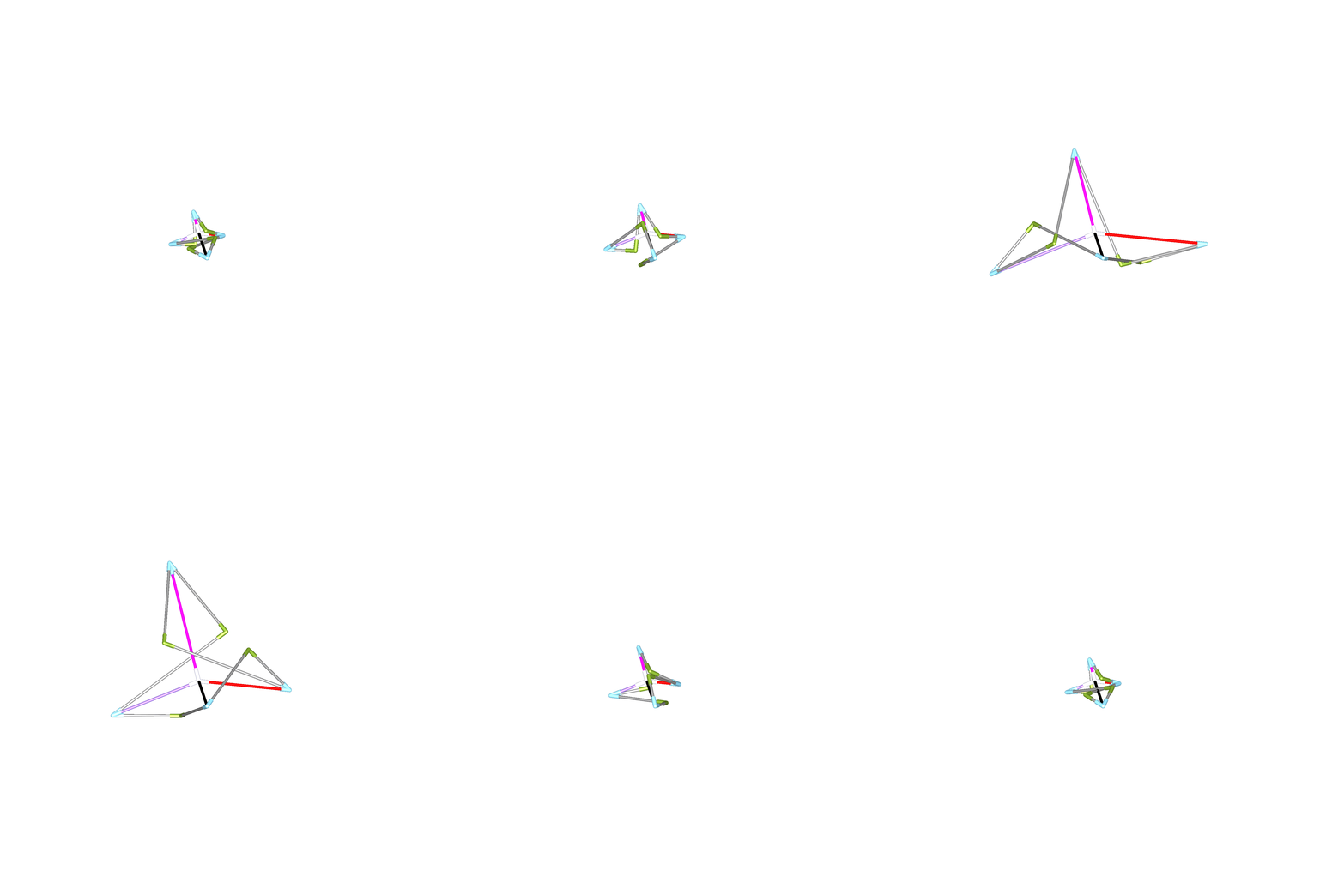
The corresponding deformation of the mesh during the continuous flexion of has to be a conformal transformation, as the vertex stars are rigid. The corresponding kinematic structure of is composed of rigid vertex stars linked by cylindrical joints (cf. Fig. 5). Note that in general such a structure only has the trivial mobility resulting from the homothetic transformation. This motion can be omitted by fixing the length of one edge in the structure. These modified linkages are in general rigid but those stemming from continuous flexible quad surfaces have an overconstrained motion.
4.2 V-hedra with skew quads
We study this class in more detail, as it is a generalization of V-hedra with planar quads having many applications to structural engineering practice [17, 24].
For the equations of Eq. (10) read as follows:
| (11) |
We can solve this set of equations explicitly for in dependence of , which yields the following two solutions:
| (12) |
with
| (13) |
Remark 2
Alternatively, the above given equations from Eq. (11) can also be solved explicitly for in dependence of , which yield the following two solutions:
| (14) |
with
| (15) |
where corresponds to the plus sign and to the minus sign.
Note that for a given skew central quad and a set of real values fulfilling the three equations , the missing geometric parameters can be computed from the equation (cf. Eq. (4)). For the minus sign we get one further real solution beside the excluded degenerate case . By shifting these two values obtained for by we obtain the solutions of the equation with respect to the plus sign. Therefore we get a unique value for with for each .
Example 2
The coordinates of the vertices of the skew central quad are given by:
| (16) |
from which the angles and for can be calculated. Moreover, the input data is completed by the values:
| (17) |
where . From that we can compute the values according to Eq. (4) with respect to the minus sign for all . Then the formulas for the solution set related to the upper sign in Eq. (12) yield
| (18) |
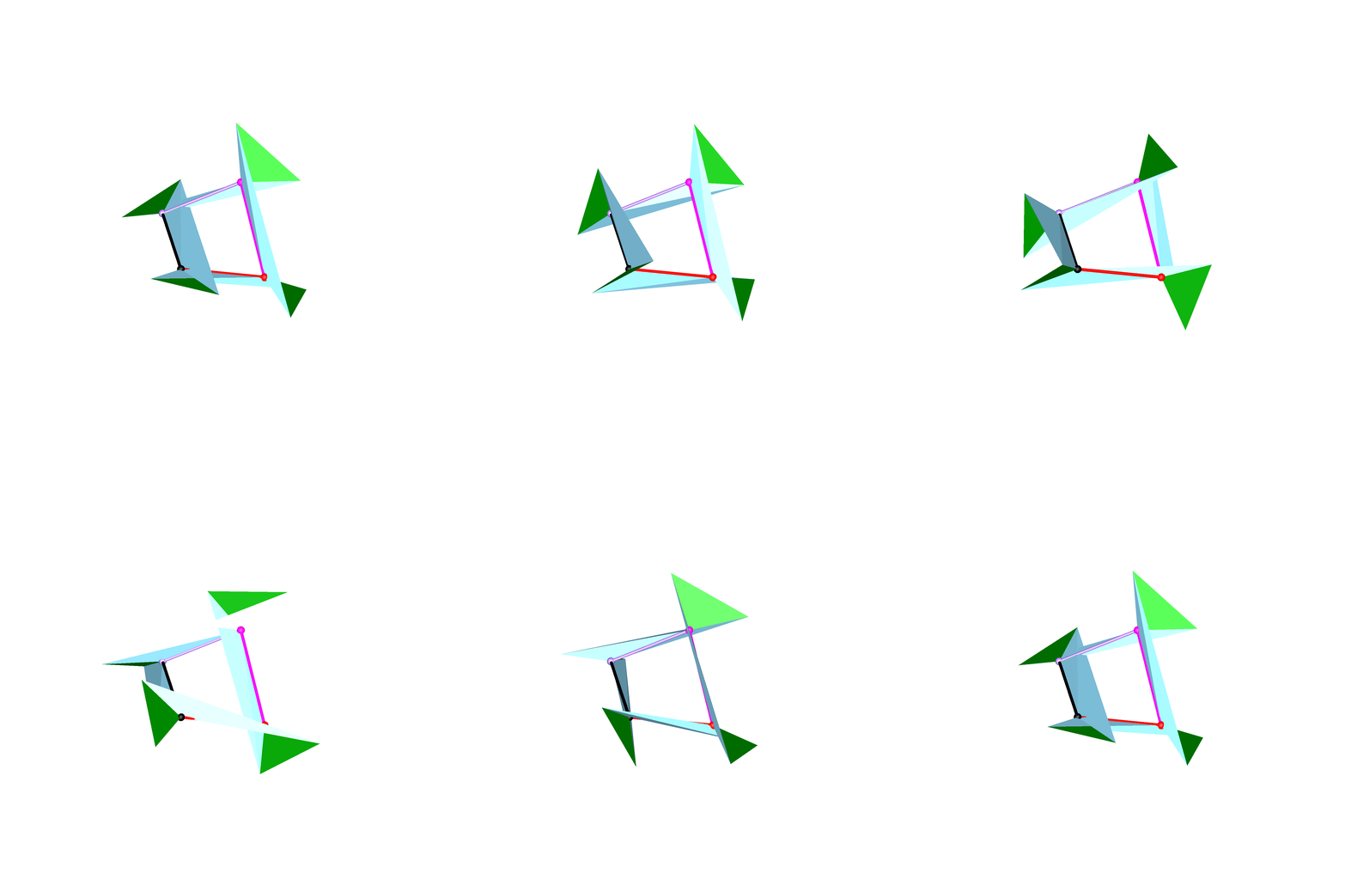
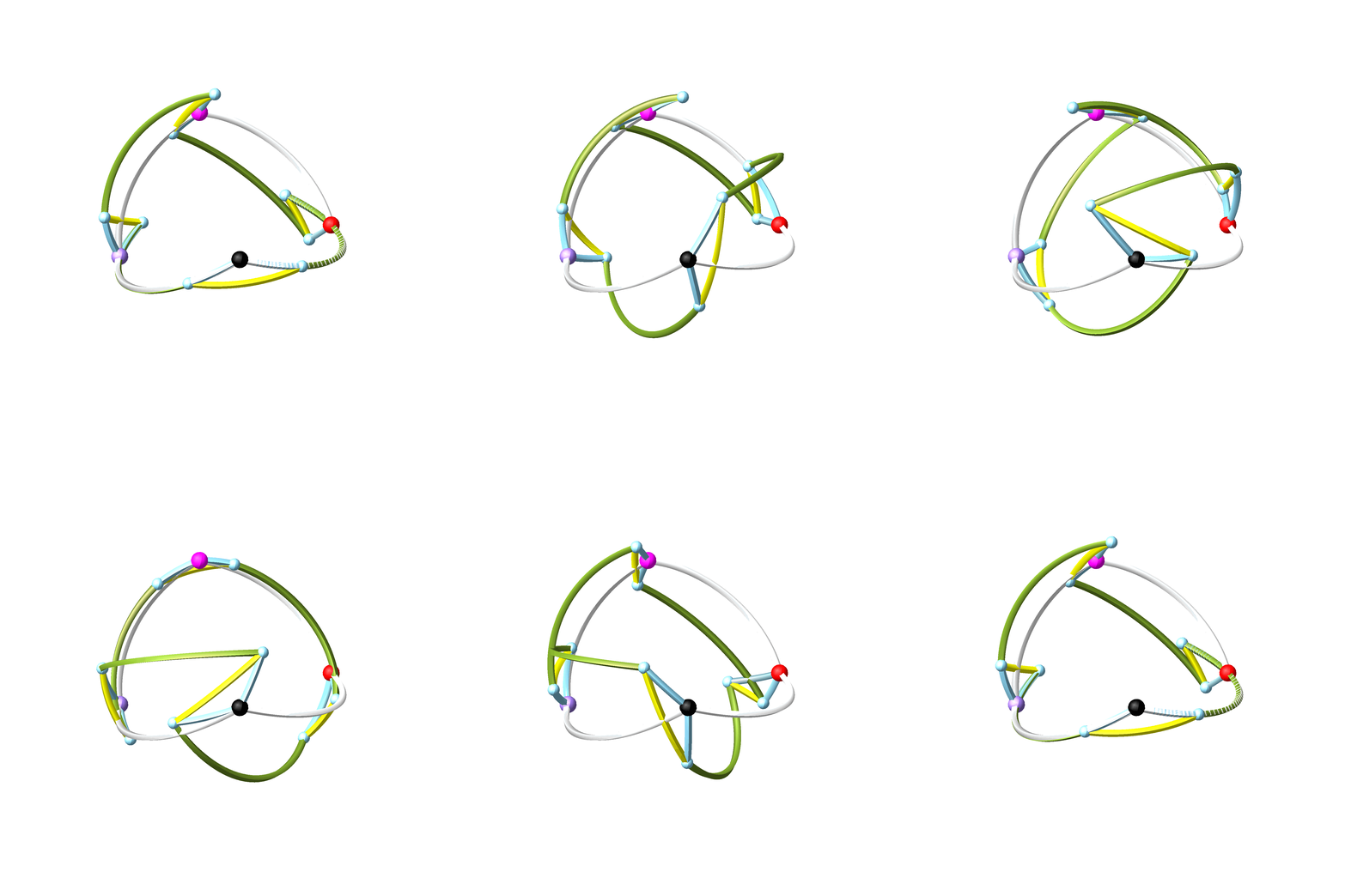
One configuration of the resulting continuous flexible building block of a V-hedra with skew quads is illustrated in Fig. 4, where also the corresponding spherical image is displayed. The associated overconstrained mechanism implied by the reciprocal-parallelism (cf. Section 4.1) is shown in Fig. 5. In the captions of Figs. 4 and 5 we also provide links to gif animations showing the overconstrained motion of these three mechanisms.
We close this section by making the following two final comments:
-
The edges of the V-hedra can be subdivided into two families of discrete parameter lines, which are called -polylines and -polylines for short. Due to the property pointed out in Section 3.1, the rotation angles along any -polyline or -polyline are the same. Note that this property is well known for V-hedra with planar quads (cf. [14, page 529]) but also holds for the skew case.
-
In view of Section 4.1 it should be noted that there is a further remarkable relation to an overconstrained mechanism beside the one illustrated in Fig. 5. As already pointed out by Sauer [15] the vertex star fulfilling the isogonality condition is reciprocal-parallel to a skew isogram, which has the following additional property: If the four bars of the isogram are hinged in the vertices by rotational joints, which are orthogonal to the plane spanned by the linked bars (cf. Fig. 6), then one obtains a so-called Bennett mechanism [25]. This is the only non-trivial mobile 4R loop.
If the quads of the V-hedra are skew then the four axes of the Bennett mechanisms, which can be associated with a vertex of the mesh , differ from each other (cf. Fig. 6). Only in the case where is a V-hedra with planar quads, each vertex of can uniquely be associated with one rotational axis orthogonal to the planar vertex star. Then the resulting network of Bennett mechanisms is highly mobile66 6 The degree of the mobility corresponds to the number of rows plus columns of minus one (cf. Sauer [15, Theorem 11.18]).. Finally it should be noted that in this case is a discrete pseudospherical surface [4, 15, 26].
5 Conclusions, open problems and future research
We generalized continuous flexible Kokotsakis belts of the isogonal type by allowing that the faces, which are adjacent to the line-segments of the rigid closed polygon , to be skew. In more detail we studied the case where is a skew quad as it corresponds to a building block of a V-hedra composed of skew quads, which proves (under consideration of Theorem 4.1) the existence of continuous flexible SQ surfaces.
Open questions in this context regard the smooth analog of continuous flexible Kokotsakis belts of the isogonal type and of V-hedra with skew quads.
This study at hand is also the starting point towards a full classification of continuous flexible SQ building blocks, which is subject to future research.
Acknowledgements.
The research is supported by grant F77 (SFB “Advanced Computational Design”, subproject SP7) of the Austrian Science Fund FWF.
References
- [1] Kokotsakis, A.: Über bewegliche Polyeder. Mathematische Annalen 107:627–647 (1932)
- [2] Karpenkov, O.N.: On the flexibility of Kokotsakis meshes. Geometriae Didicata 147:15–28 (2010)
- [3] Voss, A.: Über diejenigen Flächen, auf denen geodätische Linien ein konjugiertes System bilden. Münchner Berichte, pp. 95–102 (1888)
- [4] Schief, W.K., Bobenko, A.I., Hoffmann, T.: On the integrability of infinitesimal and finite deformations of polyhedral surfaces. Discrete Differential Geometry (A.I. Bobenko et al. eds.), Oberwolfach Seminars 38:67–93 (2008)
- [5] Evans, T.A., Lang, R.J., Magleby, S.P., Howell, L.L.: Rigidly foldable origami twists. Origami6, I: Mathematics (K. Miura et al. eds.), pp. 119–130, American Mathematical Society (2015)
- [6] Stachel, H.: A kinematic approach to Kokotsakis meshes. Computer Aided Geometric Design 27:428–437 (2010)
- [7] Bricard, R.: Mémoire sur la théorie de l’octaèdre articulé. Journal de Mathématiques pures et appliquées, Liouville 3:113–148 (1897)
- [8] Stachel, H.: Remarks on Bricard’s flexible octahedra of type 3. Proceedings of the 10th International Conference on Geometry and Graphics (July 28 - Aug. 3, 2002, Kiev/Ukraine), 1:8–12 (2002)
- [9] Nawratil, G.: Flexible octahedra in the projective extension of the Euclidean 3-space. Journal for Geometry and Graphics 14(2):147–169 (2010)
- [10] Nawratil, G., Stachel, H.: Composition of spherical four-bar-mechanisms. New Trends in Mechanisms Science – Analysis & Design (D. Pisla et al. eds.), pp. 99–106, Springer (2010)
- [11] Nawratil, G.: Reducible compositions of spherical four-bar linkages with a spherical coupler component. Mechanism and Machine Theory 46(5):725–742 (2011)
- [12] Nawratil, G.: Reducible compositions of spherical four-bar linkages without a spherical coupler component. Mechanism and Machine Theory 49:87–103 (2012)
- [13] Izmestiev, I.: Classification of flexible Kokotsakis polyhedra with quadrangular base. International Mathematics Research Notices 2017(3):715–808 (2017)
- [14] Sauer, R., Graf, H.: Über Flächenverbiegung in Analogie zur Verknickung offener Facettenflache. Mathematische Annalen 105:499–535 (1931)
- [15] Sauer, R.: Differenzengeometrie. Springer (1970)
- [16] Sharifmoghaddam, K., Nawratil, G., Rasoulzadeh, A., Tervooren, J.: Using Flexible Trapezoidal Quad-Surfaces for Transformable Design. Proceedings of the IASS Annual Symposium 2020/21 and the 7th International Conference on Spatial Structures, IASS (in press)
- [17] Montagne, N., Douthe, C., Tellier, X., Fivet, C., Baverel, O.: Voss surfaces: a design space for geodesic gridshells. Journal of the International Association for Shell and Spatial Structures 61(206):255–263 (2020)
- [18] Tachi, T.: Generalization of rigid foldable quadrilateral mesh origami. Journal of the International Association for Shell and Spatial Structures 50(3):173–179 (2009)
- [19] Tachi, T.: Freeform Rigid-Foldable Structure using Bidirectionally Flat-Foldable Planar Quadrilateral Mesh. Advances in Architectural Geometry (C. Ceccato et al. eds.), pp. 87–102, Springer (2010)
- [20] Feng, F., Dang, X., James, R.D., Plucinsky, P.: The designs and deformations of rigidly and flat-foldable quadrilateral mesh origami. Journal of the Mechanics and Physics of Solids 142:104018 (2020)
- [21] Dang, X., Feng, F., Plucinsky, P., James, R.D., Duan, H., Wang, J.: Inverse design of deployable origami structures that approximate a general surface. International Journal of Solids and Structures 234-235:111224 (2022)
- [22] Jiang, C., Wang, H., Inza, V.C., Dellinger, F., Rist, F., Wallner, J., Pottmann, H.: Using isometries for computational design and fabrication. ACM Transactions on Graphics 40(4):42 (2021)
- [23] Li, Z., Schicho, J.: Classification of angle-symmetric 6R linkages. Mechanism and Machine Theory 70:372–379 (2013)
- [24] Mitchell, T., Mazurek, A., Hartz, C., Miki, M., Baker, W.: Structural Applications of the Graphic Statics and Static-Kinematic Dualities: Rigid Origami, Self-Centering Cable Nets, and Linkage Meshes. Proceedings of the IASS Annual Symposium (July 16-20, 2018, Boston/USA), Symposium: Graphic statics, pp. 1-8(8) (2018)
- [25] Bennett, G.T.: The skew isogram mechanism. Proceedings of the London Mathematical Society s2-13(1):151–173 (1914)
- [26] Wunderlich, W.: Zur Differenzengeometrie der Flächen konstanter negativer Krümmung. Sitzungsbericht der Österreichischen Akademie der Wissenschaften, Mathem.-Naturw. Klasse IIa 160(1-5):39–77 (1951)