Coronal Mass Ejection image edge detection in Heliospheric Imager STEREO SECCHI data

Studying and monitoring solar activity, and in particular, its stronger radiation and particle emission, is important for both science and practical purpose, for our life on and around Earth. In particular, Coronal Mass Ejections (CME), which carry magnetized plasma, can induce geomagnetic storms on our planet, and also endanger astronauts or space equipment. Increased interest in studying their origins, structure, and trajectories resulted in more and more international space missions, among which several ones are still operational. The STEREO pair A and B of NASA spacecraft, out of which STEREO-B was lost in 2014, is one of such latest missions, continuously imaging the Sun and the space between Sun and Earth, with several instruments, as described in [Eyles et al.(2009)Eyles, Harrison, Davis, Waltham, Shaughnessy, Mapson-Menard, Bewsher, Crothers, Davies, Simnett, Howard, Moses, Newmark, Socker, Halain, Defise, Mazy, & Rochus, Eyles et al.(2007)Eyles, Davis, Harrison, Waltham, Halain, Mazy, Defise, Howard, Moses, Newmark, & Plunkett] by orbiting around the Sun at roughly the same distance as the Earth. Early years of raw and processed image data are available from both, and STEREO-A is still operational. Two visible-light cameras HI-1 and HI-2 on each spacecraft are thus precisely aimed in order to cover the line Sun-Earth, while being shielded from the Sun itself. Their images show various parts of the solar corona, receiving free-electron scattered light from the K-corona, dust scattered light from the F-corona, as well as light from background stars. Many studies of these images start from running differences, as described by [Sheeley et al.(1997)Sheeley, Wang, Hawley, Brueckner, Dere, Howard, Koomen, Korendyke, Michels, Paswaters, Socker, St. Cyr, Wang, Lamy, Llebaria, Schwenn, Simnett, Plunkett, & Biesecker] for coronagraph images, to enhance the faint K-corona light and remove the slowly-varying but much stronger F-corona light, as also explained in [Davies et al.(2009)Davies, Harrison, Rouillard, Sheeley, Perry, Bewsher, Davis, Eyles, Crothers, & Brown]. CME perturb the K-corona, and thus appear as bright regions in these images. Successive images, obtained from space missions such as the SOHO LASCO [Yashiro et al.(2004)Yashiro, Gopalswamy, Michalek, St. Cyr, Plunkett, Rich, & Howard], and STEREO coronagraph and HI cameras, show their propagation and evolution. Considerable research studying the origin of CMEs, shape, and trajectories is in progress, but open problems remain, as described in the very comprehensive review from [Webb & Howard(2012)], in particular regarding propelling forces and interaction with solar wind: such models can be found in [Xie et al.(2006)Xie, Gopalswamy, Ofman, St. Cyr, Michalek, Lara, & Yashiro, Michalek et al.(2006)Michalek, Gopalswamy, Lara, & Yashiro, Gopalswamy & Yashiro(2007), Howard et al.(2008)Howard, Nandy, & Koepke]. Given the large amount of data as well as the need for tracking, computerized pre-analysis tools can provide important help, in particular to identify the CME boundaries and kinematics.

Computer algorithms able to identify boundaries of various objects in images have been already studied. They can use gradient techniques such as in [Canny(1986)], or active contour techniques: [Caselles et al.(1993)Caselles, Catté, Coll, & Dibos, Chan & Vese(2001), Márquez-Neila et al.(2014)Márquez-Neila, Baumela, & Alvarez]. However, as [Young & Gallagher(2008)] explain, it is not straightforward to use these existing techniques because of the diffuse nature of CMEs. Moreover, they also have complex inner features, and their signal can be affected by the presence of bright stars and even the Milky Way passing in the field of view, which adds to the noise.

Thus, several complex algorithmic methods specialized for this task have been devised: CACTus [Robbrecht & Berghmans(2004)], SEEDS [Olmedo et al.(2008)Olmedo, Zhang, Wechsler, Poland, & Borne], and multiscale wavelet analysis [Young & Gallagher(2008), Byrne et al.(2009)Byrne, Gallagher, McAteer, & Young], mainly focused on the coronagraph images. These methods isolate the regions of interest in specific ways, and then estimate geometric and kinematic parameters, using underlying assumptions such as constant acceleration and elliptical shapes.

The algorithm presented here only focuses on the image segmentation stage, identifying the outer edge of CME regions in STEREO HI images using a staged approach composed of simple steps. The algorithm starts by filtering and smoothing the image difference, subsequently exploring it from the center of the bright CME region, marking its outer edges.

Through subsequent work, it can be integrated into various kinematic estimation schemes. Given its modular nature, the algorithm itself could also be further adapted to examine specific internal features apparent in the images.

The rest of the paper is organized as follows. In Section 2 we describe the algorithm outline and its subsequent processing of an image. In Section 3 we show its results on several other STEREO HI-1 images of known CME, and in Section 4 we discuss future lines of work.

In Figure 1 we see an example of what the algorithm starts with, which is an early phase of a CME visible in the differenced image from December 12, 2008. The Sun is behind the right edge of the image, which has $n_{c}\times n_{r}=1024\times 1024$ pixels.

The main steps, graphically illustrated in Figure 2, are as follows, where $I[c,r]$ represents the pixel intensity for coordinates column $c$ and row $r$ of the input image. The origin is the bottom left of the image.

1. 1.

   Find the center of mass $(x_{S},y_{S})$ of the bright area and set $C=(c_{S},y_{S})$ where $c_{S}$ is close to the image edge $c_{0}$ towards the Sun (right for spacecraft A, so typically $c_{0}=1023$, and left for B, i.e. $c_{0}=0$).

2. 2.

   Going from $c_{S}$ to $c_{E}$ (1023 for B, 0 for A), on each image row $r$, mark the farthest bright pixels seen along. Then do the same on each image column $c$, first from $y_{S}$ up, and then from $y_{S}$ down, with $t_{1}=240$ for 0-255 gray level images.

   1: $e_{1}\leftarrow[]$

   2: for each image row $r$ do

   3:   $q\leftarrow$False

   4:   $v\leftarrow c_{0}$

   5:   for each image column $c$ from $c_{S}$ to $c_{E}$ do

   6:    if $I[c,r]>t_{1}$ then

   7:      $v\leftarrow c$

   8:      $q\leftarrow$True

   9:    end if

   10:   end for

   11:   if $q$ then

   12:    $e_{1}+\leftarrow[v,r]$

   13:   end if

   14: end for

   15: for each image column $c$ do

   16:   for each image row $r$ from $y_{S}$ to $r_{E}$ do

   17:    if $I[c,r]>t_{1}$ then

   18:      $v\leftarrow r$

   19:      $q\leftarrow$True

   20:    end if

   21:   end for

   22:   if $q$ then

   23:    $e_{1}+\leftarrow[c,v]$

   24:   end if

   25:   for each image row $r$ from $y_{S}$ to $0$ do

   26:    if $I[c,r]>t_{1}$ then

   27:      $v\leftarrow r$

   28:      $q\leftarrow$True

   29:    end if

   30:   end for

   31:   if $q$ then

   32:    $e_{1}+\leftarrow[c,v]$

   33:   end if

   34: end for
3. 3.

   Smooth the image $I$ into $I_{M}$, using a sum-scale-and-modulo-256 5x5 filter to enhance contrast at the edges

4. 4.

   Mark the contrasting pixels created in step 3, with $t_{2}=120$ for 0-255 gray level images

   1: $e_{2}\leftarrow[]$

   2: for each image row $r$ do

   3:   for each image column $c$ except the last one do

   4:    if $|I_{M}[c,r]-I_{M}[c+1,r]|>t_{2}$ then

   5:      $e_{2}+\leftarrow[c,r]$

   6:    end if

   7:   end for

   8: end for

   9: for each image column $c$ do

   10:   for each image row $r$ except the last one do

   11:    if $|I_{M}[c,r]-I_{M}[c,r+1]|>t_{2}$ then

   12:      $e_{2}+\leftarrow[c,r]$

   13:    end if

   14:   end for

   15: end for
5. 5.

   Mark the centers where both kinds of previous marks are present in a $w_{i}\times w_{i}$ window, as created in step 2 and step 4, namely from the $e_{1}$ and $e_{2}$ lists:

   1: $I_{1}=\textrm{ones}[n_{c},n_{r}]$

   2: $I_{2}=\textrm{ones}[n_{c},n_{r}]$

   3: for each element $[x,y]$ of $e_{1}$ do

   4:   $I_{1}[x,y]\leftarrow 2$

   5: end for

   6: for each element $[x,y]$ of $e_{2}$ do

   7:   $I_{2}[x,y]\leftarrow 3$

   8: end for

   9: $I_{3}\leftarrow I_{1}+I_{2}$

   10: $I_{4}\leftarrow\textrm{filter}(I_{3},\textrm{prod},w_{i})$

   11: $e_{3}\leftarrow$ list of $[x,y]$ such that $I_{4}[x,y]$ is a multiple of $2$ and $3$, or of $5$
6. 6.

   Estimate the density of the markers from step 5 in a larger window $w_{d}\times w_{d}$ and mark those above half into a boolean mask $I_{D}$.

7. 7.

   Circularly sweeping from the center, for each such radial half-line gather the last mark as created in step 6, i.e. from $I_{D}$, and build the perimeter:

   1: $e_{4}\leftarrow[]$

   2: for each angle $\alpha$ from $0$ to $2\pi$ in steps of $\varepsilon$ do

   3:   $v\leftarrow$Nothing

   4:   for each pixel $[x,y]$ along the $\alpha$ ray from $[c_{S},y_{S}]$ to any edge of the image do

   5:    if $I_{D}[x,y]$ then

   6:      $v\leftarrow[x,y]$

   7:    end if

   8:   end for

   9:   if $v$ then

   10:    $e_{4}+\leftarrow v$

   11:   end if

   12: end for
8. 8.

   Remove spikes (outliers) created in step 7 in the list $e_{4}$ of pairs of pixel coordinates, reconnect and validate the final perimeter, based on CME geometry from [Fisher(1984), Fisher & Munro(1984), Crifo(1983)].

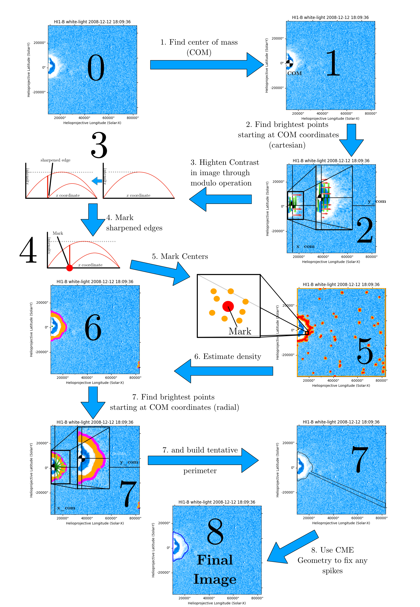
The idea behind step 3 is to augment existing gradual contrasting zones by creating an abrupt transition through the modulo operation.

Given the larger density of markers around the true edge, even if the rays in step 7 are one or two pixels wide, they should not miss them when they cross it outwards.

Outliers appear occasionally because of brighter background light points far away from the CM, and can be removed in step 8. The validation of the perimeter, to eliminate unphysical results, is based on CME general geometry, using bubble and loop models as described in [Crifo(1983)]. Specifically, as [Fisher(1984)] and [Fisher(1984)] point out, the width to depth ratio is typically 3:2, so we compute and compare these diameters.

We have tracked CME events using a set of 100 STEREO 11-day background-removed L2 HI-1 a and b images from the UK Solar System Data Center, https://www.ukssdc.ac.uk. The algorithm performed with overall high tracking capabilities and without any fine-tuning or training set. We also conducted a manual identification of the CME regions, and then compared it with the automatic one. We counted the relative differences in areas between the two perimeters as errors, and we measured by hand that the percentage error of region identifications was below 15% for the most irregular events. We did not find false positives. The images in Figure 3 and Figure 5 illustrate these cases.

A simplified initial calculation appears in agreement with speeds of the order of $300$km/s from [Davis et al.(2009)Davis, Davies, Lockwood, Rouillard, Eyles, & Harrison] for the 2008 December 12 CME event, as effectively measured by the SWEPAM instrument aboard the Advanced Composition Explorer spacecraft [Stone et al.(1998)Stone, Frandsen, Mewaldt, Christian, Margolies, Ormes, & Snow]. We used the transformation (4) described in [Thompson(2006)]:

to compute the displacement of the front, from the Helioprojective longitude displacement of $\theta_{x}=0.27^{\circ}=1000$ seconds of arc from 18:09 to 18:49 of two algorithm-generated contours for HI-1 B, shown in Figure 4. Thus, $\Delta x=730000$km, and $\Delta t=2400s$, so $v=300$km/s, using only two significant digits.

Succesive images, such as in Figure 5 can allow more accurate estimations of kinematics.

To improve the smoothness and completeness of the perimeter detection, we have also tried a subsequent stage of the morphological geodesic active contour method from [Márquez-Neila et al.(2014)Márquez-Neila, Baumela, & Alvarez], based on level sets seeded with the interior of an initially-found contour. So far, it did not seem to succeed, mainly because of the of the various bright-dark alternating inner fronts, and also because of the background noise from the light of the stars. The latter could be further reduced by carefully realigning the images before subtraction, as suggested by [Davies et al.(2009)Davies, Harrison, Rouillard, Sheeley, Perry, Bewsher, Davis, Eyles, Crothers, & Brown].

A possible line of improvement would be to better adapt the active contour methods to the already-found contour to fine-align it along less-contrasting borders. A more precise way to distinguish the far-away background could also help. Finally, I am planning on working to integrate it with existing models to estimate CME velocities and 3D shape changes, and then systematically comparing it with other methods.

We have implemented the algorithm in Python, and made it available at https://github.com/MDNich/CME-Image-Edge-Detection-in-Python-from-STEREO-data, being thus grateful to the community maintaining Numpy, SciPy and Matplotlib, as well as [The SunPy Community et al.(2020)The SunPy Community, Barnes, Bobra, Christe, Freij, Hayes, Ireland, Mumford, Perez-Suarez, Ryan, Shih, Chanda, Glogowski, Hewett, Hughitt, Hill, Hiware, Inglis, Kirk, Konge, Mason, Maloney, Murray, Panda, Park, Pereira, Reardon, Savage, Sipőcz, Stansby, Jain, Taylor, Yadav, Rajul, & Dang]. We thank the reviewers for their careful reading and helpful comments and for suggestions for applications of these techniques to missions such as PUNCH and Solar Orbiter.

References

- [Byrne et al.(2009)Byrne, Gallagher, McAteer, & Young] Byrne, J. P., Gallagher, P. T., McAteer, R. T. J., & Young, C. A. 2009, A&A, 495, 325
- [Canny(1986)] Canny, J. 1986, IEEE Transactions on Pattern Analysis and Machine Intelligence, 8, 679
- [Caselles et al.(1993)Caselles, Catté, Coll, & Dibos] Caselles, V., Catté, F., Coll, T., & Dibos, F. 1993, Numer. Math., 66, 1
- [Chan & Vese(2001)] Chan, T. F. & Vese, L. A. 2001, IEEE Transactions on Image Processing, 10, 266
- [Crifo(1983)] Crifo, F. 1983, Solar Physics, 83, 143
- [Davies et al.(2009)Davies, Harrison, Rouillard, Sheeley, Perry, Bewsher, Davis, Eyles, Crothers, & Brown] Davies, J. A., Harrison, R. A., Rouillard, A. P., et al. 2009, Geophys. Res. Lett., 36, L02102
- [Davis et al.(2009)Davis, Davies, Lockwood, Rouillard, Eyles, & Harrison] Davis, C. J., Davies, J. A., Lockwood, M., et al. 2009, Geophys. Res. Lett., 36, L08102
- [Eyles et al.(2007)Eyles, Davis, Harrison, Waltham, Halain, Mazy, Defise, Howard, Moses, Newmark, & Plunkett] Eyles, C., Davis, C., Harrison, R., et al. 2007, in Solar Physics and Space Weather Instrumentation II, ed. S. Fineschi & R. A. Viereck, Vol. 6689, International Society for Optics and Photonics (SPIE), 40 – 52
- [Eyles et al.(2009)Eyles, Harrison, Davis, Waltham, Shaughnessy, Mapson-Menard, Bewsher, Crothers, Davies, Simnett, Howard, Moses, Newmark, Socker, Halain, Defise, Mazy, & Rochus] Eyles, C. J., Harrison, R. A., Davis, C. J., et al. 2009, Sol. Phys., 254, 387
- [Fisher(1984)] Fisher, R. 1984, Adv. Space Res., 4, 163
- [Fisher & Munro(1984)] Fisher, R. & Munro, H. R. 1984, Astrophys. J., 280, 163
- [Gopalswamy & Yashiro(2007)] Gopalswamy, N. & Yashiro, S. 2007, Journal of Geophysical Research, 112
- [Howard et al.(2008)Howard, Nandy, & Koepke] Howard, T., Nandy, D., & Koepke, A. 2008, Journal of Geophysical Research, 113
- [Michalek et al.(2006)Michalek, Gopalswamy, Lara, & Yashiro] Michalek, G., Gopalswamy, N., Lara, A., & Yashiro, S. 2006, Space Weather, 4, S10003
- [Márquez-Neila et al.(2014)Márquez-Neila, Baumela, & Alvarez] Márquez-Neila, P., Baumela, L., & Alvarez, L. 2014, IEEE Transactions on Pattern Analysis and Machine Intelligence, 36, 2
- [Olmedo et al.(2008)Olmedo, Zhang, Wechsler, Poland, & Borne] Olmedo, O., Zhang, J., Wechsler, H., Poland, A., & Borne, K. 2008, in AGU Spring Meeting Abstracts, Vol. 2008, SP43A–02
- [Robbrecht & Berghmans(2004)] Robbrecht, E. & Berghmans, D. 2004, A&A, 425, 1097
- [Sheeley et al.(1997)Sheeley, Wang, Hawley, Brueckner, Dere, Howard, Koomen, Korendyke, Michels, Paswaters, Socker, St. Cyr, Wang, Lamy, Llebaria, Schwenn, Simnett, Plunkett, & Biesecker] Sheeley, N. R., Wang, Y. M., Hawley, S. H., et al. 1997, ApJ, 484, 472
- [Stone et al.(1998)Stone, Frandsen, Mewaldt, Christian, Margolies, Ormes, & Snow] Stone, E. C., Frandsen, A. M., Mewaldt, R. A., et al. 1998, Space Sci. Rev., 86, 1
- [The SunPy Community et al.(2020)The SunPy Community, Barnes, Bobra, Christe, Freij, Hayes, Ireland, Mumford, Perez-Suarez, Ryan, Shih, Chanda, Glogowski, Hewett, Hughitt, Hill, Hiware, Inglis, Kirk, Konge, Mason, Maloney, Murray, Panda, Park, Pereira, Reardon, Savage, Sipőcz, Stansby, Jain, Taylor, Yadav, Rajul, & Dang] The SunPy Community, Barnes, W. T., Bobra, M. G., et al. 2020, The Astrophysical Journal, 890, 68
- [Thompson(2006)] Thompson, W. T. 2006, Astronomy and Astrophysics, 449, 791
- [Webb & Howard(2012)] Webb, D. F. & Howard, T. A. 2012, Living Reviews in Solar Physics, 9
- [Xie et al.(2006)Xie, Gopalswamy, Ofman, St. Cyr, Michalek, Lara, & Yashiro] Xie, H., Gopalswamy, N., Ofman, L., et al. 2006, Space Weather, 4, S10002
- [Yashiro et al.(2004)Yashiro, Gopalswamy, Michalek, St. Cyr, Plunkett, Rich, & Howard] Yashiro, S., Gopalswamy, N., Michalek, G., et al. 2004, Journal of Geophysical Research (Space Physics), 109, A07105
- [Young & Gallagher(2008)] Young, C. A. & Gallagher, P. T. 2008, Sol. Phys., 248, 457