GIGA-Lens: Fast Bayesian Inference for Strong Gravitational Lens ModelingJournal: ApJ TensorFlow (Abadi et al. 2015), TensorFlow Probability (Dillon et al. 2017), JAX (Bradbury et al. 2018), Optax (Hessel et al. 2020), lenstronomy (Birrer & Amara 2018), emcee (Foreman-Mackey et al. 2013), Matplotlib (Hunter 2007), seaborn (Waskom 2021), corner.py (Foreman-Mackey 2016), TinyTim (Krist et al. 2011), NumPy (Harris et al. 2020)

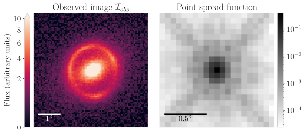
Given a lens model fully described by a set of parameters $\Theta$, the predicted counts per second at arbitrary positions on the image plane, $\mathcal{I}_{model}(x,y;\Theta)$, can be determined by evaluating the deflection angle at $(x,y)$, using this deflection to ray trace (Narayan & Bartelmann 1997, e.g.,) onto the source plane, setting the surface brightness of the lensed source at $(x,y)$ to the corresponding surface brightness on the source plane (via surface brightness conservation), then adding the lens light, and finally convolving with the PSF²² 2 The sky brightness, $I_{sky}$, can also be included in the model parameters $\Theta$. In this work, we assume the sky brightness has been subtracted.. To demonstrate how our modeling pipeline works, we simulate a reference system (Fig. 1) using lenstronomy. The lens model used for this simulation consists of an elliptical power law³³ 3 We note the EPL model is equivalent to the power law elliptical mass density profile (Barkana 1998, PEMD;). (EPL) mass model for the lens (Tessore & Metcalf 2015) and external shear. The EPL model is characterized by the surface mass density in units of the critical density, or convergence,

where $\theta_{E}$ is the Einstein radius, $\gamma_{epl}$ is the mass profile slope, the coordinates $x_{{\color[rgb]{0,0,0}lens}},y_{{\color[rgb]{0,0,0}lens}}$ are aligned with the major and minor axes of the lens, and $q$ is the axial ratio. The transformation between the image coordinates $(x,y)$ and the lens-centric coordinates $(x_{lens},y_{lens})$ is

where $\phi$ is the position angle and $x_{epl}$ and $y_{epl}$ are the lens center. The deflection angle for this model can be written in terms of the Gaussian hypergeometric function, which can be calculated iteratively, converging to a high degree of accuracy in a small number of iterations. The truncation error reaches $\lesssim 10^{-16}$ within 35 iterations for $q\gtrsim 0.5$ (Tessore & Metcalf 2015).

To include the effects of the local environment, we include an external shear with a deflection angle

Finally, for our simulations, we model our lens and source light with an elliptical Sérsic profile (Sérsic 1963):

where $b_{n}=1.9992n-0.3271$, $R_{eff}$ is the effective radius (half-light radius), $n$ is the Sérsic index, and $x_{{\color[rgb]{0,0,0}light}},y_{{\color[rgb]{0,0,0}light}}$ are aligned with the major and minor axes of the light profile. The transformation between image coordinates $(x,y)$ and light coordinates $(x_{light},y_{light})$ is identical in form to Eq. 2. We will use $(x_{l},y_{l})$ to denote the lens light center (in this work, the lens light center is not fixed to the lens mass center) and $(x_{s},y_{s})$ to denote the source light center. Finally, in lens modeling, eccentricities are often used through the reparameterization,

where $\phi$ is the position angle. We will use $(\epsilon_{epl,1},\epsilon_{epl,2})$ to denote the lens mass eccentricities, $(\epsilon_{l,1},\epsilon_{l,2})$ for the lens light eccentricities, and $(\epsilon_{s,1},\epsilon_{s,2})$ for the source light eccentricities. Similarly, $R_{l}$ and $R_{s}$ will denote the lens and source light effective radius.

In practice, $\mathcal{I}_{model}(x,y;\Theta)$ is vectorized to be evaluated on a grid of pixels simultaneously. This grid is supersampled by some integer factor $k_{super}$ (in this work, $k_{super}=2$) from the image coordinates, so there is an additional step in evaluating $\mathcal{I}_{model}$ that consists of downsampling (by averaging) the predicted image by $k_{super}$ back to the image coordinate grid.

Our probabilistic model comprises a likelihood function $\mathcal{L}(\Theta;\mathcal{I}_{obs})\equiv p(\mathcal{I}_{obs}\mid\Theta)$ and a prior $p(\Theta)$, where $\Theta\in\mathbb{R}^{d}$ are the lensing system parameters, and $\mathcal{I}_{obs}$ is the observed image (in units of counts/sec). The likelihood function requires a preprocessed observed image $\mathcal{I}_{obs}$ as well as specification of the background (sky) Gaussian noise $\sigma_{bkg}$ and exposure time $t_{exp}$. For this work, we define:

where $\mathcal{I}_{model}(x,y;\Theta)$ is our forward model for the observed image, $\mathcal{G}$ is the gain (in $\mathrm{e^{-}}$/count), and the sum is over all pixels $(x,y)$ in the observed data. The second term in the variance map arises from Poisson shot noise: since the expected value of the electron counts is $t_{exp}\mathcal{I}_{model}\mathcal{G}$, the Poisson variance is therefore also $t_{exp}\mathcal{I}_{model}\mathcal{G}$, and so the Poisson variance of the model image is $\frac{t_{exp}\mathcal{I}_{model}\mathcal{G}}{\mathcal{G}^{2}\cdot t_{exp}^{2}}=\frac{\mathcal{I}_{model}}{\mathcal{G}\cdot t_{exp}}$. The form of this likelihood assumes independent per-pixel noise. However, the variance map $\sigma_{tot}^{2}$ can be specified to account for correlated pixels and to incorporate prior information about the noise at each pixel. For example, an alternative form for $\sigma_{tot}^{2}$, defined in terms of the observed image, is sometimes used: $\sigma_{tot}^{2}(x,y)=\sigma^{2}_{bkg}+\frac{\mathcal{I}_{obs}(x,y)}{\mathcal{G}\cdot t_{exp}}$ , so that the total variance is independent of $\Theta$. This is done for computational efficiency. For example, it allows for linear light profile parameters to be solved for in closed form. We note, however, this definition for the variance may induce biases at low signal-to-noise ratios (Horne 1986).⁴⁴ 4 Another issue with using $\mathcal{I}_{obs}$ to define the noise map $\sigma^{2}_{tot}$ is that it may have negative pixel values due to Gaussian noise. In lenstronomy, the negative pixels are set to zero, which is not the most rigorous way to estimate the Poisson noise. Despite the slight difference in these two approaches, for our simulated systems (§III), the results using both are virtually identical. Therefore, we opt to use the more rigorous definition. In our pipeline, this incurs little additional computational cost. We also point out that the first term in the log-likelihood corresponds to

and the second term is the normalization factor.

The prior for the parameters is typically defined as a product of independent distributions, each of which can be tuned either to reflect prior knowledge about lensing parameters, or to match a physical understanding of the particular system that is being modelled (e.g., the Einstein radius can typically be estimated to within 20% from visual inspection). Given our physical understanding of the model, our prior ought to vanish for certain regions of parameter space, such as $\theta_{E}<0$. In our modeling, we make use of mappings that naturally enforce these constraints. We describe these mappings in §II.2.

In this work, we use a “simulation distribution” to generate a full set of 22 parameters for 100 lensing systems, and the prior distribution used to model these lenses (see §III) is a broadened version of this simulation distribution (note some rows contain two parameters):

where $\mathcal{U}(a,b)$ is a uniform distribution with support $\quantity[a,b]$, $\mathcal{N}(\mu,\sigma)$ is Gaussian with mean $\mu$ and standard deviation $\sigma$, and $\mathcal{TN}(\mu,\sigma;x_{low},x_{high})$ is a truncated Gaussian with support $\quantity[x_{low}, x_{high}]$. For the distribution parameters, we use the notation ${\color[rgb]{1,0,0}a}\ /\ {\color[rgb]{0,0,1}b}$ to indicate that the simulation distribution uses the parameter ${\color[rgb]{1,0,0}a}$ while the prior uses ${\color[rgb]{0,0,1}b}$. For instance, when generating our dataset, we sample $x_{epl}$ from $\mathcal{N}(0,0.03)$, while during modeling, our prior for $x_{epl}$ is $\mathcal{N}(0,0.06)$.

Note that $\exp(\mathcal{N}(\ldots))$ is a log-normal distribution, used for 5 parameters. Since these distributions are not as intuitive, we show them in Fig. 2. The simulation distribution for the light amplitudes $I_{l}$ and $I_{s}$ have been chosen in such a way that the typical signal-to-noise ratio of the arcs is 100 (with a range between 30 and 200), and is comparable to the amplitudes used in the lenstronomy starting guide Jupyter Notebook (Birrer 2021).

Although the distributions in Eq. 8 can be specified in any format, in this work, we make a number of deliberate choices. Most importantly, for parameters such as ellipticities (e.g., $\epsilon_{epl,1},\epsilon_{epl,2}$) and centers (e.g., $x_{epl},y_{epl}$), we use normal distributions to reflect their rotational symmetry. For instance, in Fig. 3, we show how a normal distribution for the ellipticities results in a uniform distribution for the position angle $\phi$, whereas independent uniform distributions for the ellipticities break rotational symmetry, resulting in a non-uniform distribution for $\phi$ and a highly non-Gaussian distributions for $q$.

We sample from the posterior $\tilde{p}(\tilde{\Theta}\mid\mathcal{I}_{obs})$ in the unconstrained parameter space with HMC and convert back to samples of the physical parameters $p(\Theta\mid\mathcal{I}_{obs})$ using the bijector $g$. We initialize $n_{HMC}$ chains¹³¹³ 13 We use multiple chains, $n_{HMC}=50$, first because our framework naturally lends itself to parallelization, so it is more efficient to sample for $750$ iterations using $50$ chains rather than sampling for $750\cdot 50$ iterations using one chain. Using multiple chains is also necessary to evaluate sampling diagnostics such as $\hat{R}$ (see end of this section). by sampling from the surrogate posterior calculated by VI (namely, $\mathcal{N}(\tilde{\mu}^{*}_{VI},\tilde{\Sigma}^{*}_{VI})$), and as is typical for Monte Carlo samplers, run $n_{burn}$ burn-in steps before sampling $n_{sample}$ times.

Correctly configuring the HMC sampler is important to realizing its advantages. There are three hyperparameters in HMC: the step size $\epsilon$, number of leapfrog steps $L$, and the mass matrix $\tilde{M}$ that defines the momentum distribution. Much work has been done to adaptively set the first two hyperparameters $\epsilon$ and $L$. We use the methods introduced by Hoffman et al. 2014; Hoffman et al. 2021, as implemented by TensorFlow Probability, to automatically tune (‘‘autotune’’) the hyperparameters during the first 80%¹⁴¹⁴ 14 As recommended by Tensorflow Probability (see https://www.tensorflow.org/probability/api_docs/python/tfp/mcmc/DualAveragingStepSizeAdaptation). of burn-in phase. They are then fixed in the remaining burn-in steps, since their adaptation generally prevents chains from reaching the stationary distribution (hence the use of only the first 80% of burn-in steps for adaptation). Part of this tuning is adjusting the step size $\epsilon$ to achieve a target acceptance probability for each proposal: a step size that is too small will result in slower sampling, but a step size that is too large will result in too many rejected proposals. Optimal values for the target acceptance probability range between 0.6 to 0.8 (Betancourt 2018); we use 0.75. The remaining hyperparameter, the mass matrix $\tilde{M}$, defines the momentum distribution, and this provides a way to inform the HMC algorithm about the scales and correlations of the parameters. We can significantly improve the sampling efficiency by setting $\tilde{M}$ to be the inverse covariance matrix of the posterior (Brooks et al. 2011, Chap. 5) — this is called “preconditioned” HMC. This was the main purpose of the previous section, §II.4: we set $\tilde{M}=(\tilde{\Sigma}^{*}_{VI})^{-1}$, the inverse of the inferred covariance matrix from VI as defined by Eq. 16. There have been proposals (Sountsov & Hoffman 2021, e.g.,) to adapt the mass matrix $\tilde{M}$ on the fly during the burn-in steps, which may render the VI step irrelevant. For now, these methods are not yet well-tested (however, they may be incorporated in future work), hence VI remains a necessary step of our modeling pipeline. Note that a secondary use of the VI step is that each of the $n_{HMC}$ chains are initialized (see Table 1) by sampling from the VI posterior, $\mathcal{N}(\tilde{\mu}_{VI}^{*},\tilde{\Sigma}_{VI}^{*})$.

We show in Section II.5.1 the posterior samples for our reference system generated using $n_{HMC}=50$ chains and $n_{burn},n_{sample}=250,750$. As with the VI step, these hyperparameters were roughly tuned on the reference system. We report two metrics that are widely used in the statistics literature to measure the degree to which our sampler has converged. These are known as the effective sample size (ESS) and potential scale reduction factor (PSRF), $\hat{R}$ (Gelman & Rubin 1992). The former measures the effective number of independent samples we have drawn from the posterior by accounting for autocorrelation within each chain, and the latter is the ratio of the average within-chain variance to the variance of the pooled samples across all chains. A large ESS and a $\hat{R}$ that is close to 1 indicates convergence has been achieved (in Gelman & Rubin 1992, it is suggested that an appropriate condition is $\hat{R}<1.1$).

Foreman-Mackey et al. 2013 implemented an affine-invariant ensemble sampler, emcee. It is a popular MCMC algorithm in astrophysics. This is the sampler that lenstronomy uses. Here we compare the performance of HMC with emcee, which is gradient-free, by applying both to the reference system (Fig. 1). To make the comparison as fair as possible, for emcee sampling, we initialize the sampler with the lenstronomy recommended configuration, as detailed in Birrer 2021, and for our HMC sampling, we initialize the sampler as detailed in Table 1. Furthermore, we run our pipeline on a single A100 GPU and emcee on a single CPU. lenstronomy uses uniform priors for each parameter whereas we use the prior described in Eq. 8. However, we have found that the difference in priors has virtually no effect on the sampling results. Finally, for both modeling pipelines, we use the supersampling factor $k_{super}=2$ and the PSF shown in Fig. 1.

We take two axes of comparison between HMC and emcee. First, we observe that our sampling process is significantly more efficient than emcee, as evidenced by the rate at which HMC generates independent samples, $\sim 40\ \text{ESS}/\text{iter}$ ($\sim 300\ \text{ESS}/\text{sec}$, on a single A100 GPU) whereas for emcee it is $\sim 0.2\ \text{ESS}/\text{iter}$ ($\sim 0.04\ \text{ESS}/\text{sec}$) (see Section II.5.2). Second, we compare the convergence of the two samplers. We find that although both sampling methods agree in terms of their central values, they exhibit dramatically different convergence behavior. In Section II.5.2, we show that individual emcee chains tend to devolve to random walks. This random walk behavior manifests itself in three ways. First, emcee makes slow progress exploring the posterior, whereas HMC draws virtually independent samples each iteration, traversing the posterior very efficiently. Second, compared with HMC, we observe high inter-chain variance in emcee, evidenced qualitatively by the differing marginal distributions for each of the individual chains, and quantitatively by the substantially higher $\hat{R}$ for emcee (Section II.5.2). Third, in Section II.5.2 we find that the autocorrelation time for HMC is much lower than that of emcee: within just 10 iterations, the autocorrelation shrinks to negligible levels, compared to emcee, which has a characteristic autocorrelation lag of $\sim 300$. The empirical autocorrelation at lag $\tau$ for a single MC chain $\quantity{f_n \mid n=1,\ldots,N}$ is defined by (Sokal 1996):

We emphasize that this autocorrelation is independent of the iteration number. That is, burn-in does not remove autocorrelation, nor does running a chain for a very long time.

Our investigation of emcee revealed undesirable characteristics even for low to moderate dimensional spaces, as shown above in the case of the reference system with $22$ parameters. While in this regime, it is possible that through tuning and longer sampling time, higher quality convergence can still be achieved using emcee, Betancourt 2018 pointed out that in higher dimensions, any gradient-free sampler is likely to be much less efficient compared with HMC. Furthermore, Huijser et al. 2017 found that in moderate ($\sim 50$) to high ($>100$) dimensions, affine-invariant ensemble samplers (such as emcee) can have more severe problems. They showed that for high dimensional posteriors, in addition to slow convergence, an affine invariant sampler can misleadingly appear to converge even when it has not. In strong lens modeling, it is critical to avoid this pernicious behavior, since models for high resolution observed data that use complex light profiles such as shapelets (Birrer et al. 2015), wavelets (Galan et al. 2021), or pixelization (Nightingale et al. 2021) can easily have $\gtrsim 50$ parameters. The modeling of perturbations to the smooth lensing potential, whether due to dark matter subhalos or line-of-sight halos will require even more. If we wish to fit these sophisticated models to observed data, we must be able to do robust inference in spaces of moderate to high dimensions.

References

- Abadi et al. (2015) Abadi, M., Agarwal, A., Barham, P., et al. 2015, TensorFlow: Large-Scale Machine Learning on Heterogeneous Systems. https://www.tensorflow.org/
- Barkana (1998) Barkana, R. 1998, ApJ, 502, 531, doi: 10.1086/305950
- Baydin et al. (2018) Baydin, A. G., Pearlmutter, B. A., Radul, A. A., & Siskind, J. M. 2018, Journal of Machine Learning Research, 18, 1. http://jmlr.org/papers/v18/17-468.html
- Betancourt (2018) Betancourt, M. 2018, A Conceptual Introduction to Hamiltonian Monte Carlo. https://arxiv.org/abs/1701.02434
- Betancourt (2015) Betancourt, M. J. 2015, Adiabatic Monte Carlo. https://arxiv.org/abs/1405.3489
- Birrer (2021) Birrer, S. 2021, lenstronomy Starting Guide. https://github.com/sibirrer/lenstronomy_extensions/blob/main/lenstronomy_extensions/Notebooks/starting_guide.ipynb
- Birrer & Amara (2018) Birrer, S., & Amara, A. 2018, Physics of the Dark Universe, 22, 189, doi: 10.1016/j.dark.2018.11.002
- Birrer et al. (2015) Birrer, S., Amara, A., & Refregier, A. 2015, ApJ, 813, 102, doi: 10.1088/0004-637x/813/2/102
- Birrer et al. (2020) Birrer, S., Shajib, A. J., Galan, A., et al. 2020, A&A, 643, A165, doi: 10.1051/0004-6361/202038861
- Blei et al. (2017) Blei, D. M., Kucukelbir, A., & McAuliffe, J. D. 2017, Journal of the American Statistical Association, 112, 859–877, doi: 10.1080/01621459.2017.1285773
- Bolton et al. (2006) Bolton, A. S., Burles, S., Koopmans, L. V. E., Treu, T., & Moustakas, L. A. 2006, ApJ, 638, 703, doi: 10.1086/498884
- Bonvin et al. (2017) Bonvin, V., Courbin, F., Suyu, S. H., et al. 2017, MNRAS, 465, 4914, doi: 10.1093/mnras/stw3006
- Bradač et al. (2008) Bradač, M., Allen, S. W., Treu, T., et al. 2008, ApJ, 687, 959–967, doi: 10.1086/591246
- Bradbury et al. (2018) Bradbury, J., Frostig, R., Hawkins, P., et al. 2018, JAX: composable transformations of Python+NumPy programs, 0.2.5. http://github.com/google/jax
- Broadhurst et al. (2000) Broadhurst, T., Huang, X., Frye, B., & Ellis, R. 2000, ApJ, 534, L15, doi: 10.1086/312651
- Brooks et al. (2011) Brooks, S., Gelman, A., Jones, G., & Meng, X.-L., eds. 2011, Handbook of Markov Chain Monte Carlo (Chapman and Hall/CRC), doi: 10.1201/b10905
- Çaǧan Şengül et al. (2021) Çaǧan Şengül, A., Dvorkin, C., Ostdiek, B., & Tsang, A. 2021, Substructure Detection Reanalyzed: Dark Perturber shown to be a Line-of-Sight Halo. https://arxiv.org/abs/2112.00749
- Çaǧan Şengül et al. (2020) Çaǧan Şengül, A., Tsang, A., Diaz Rivero, A., et al. 2020, Phys. Rev. D, 102, 063502, doi: 10.1103/PhysRevD.102.063502
- Cañameras et al. (2020) Cañameras, R., Schuldt, S., Suyu, S. H., et al. 2020, A&A, 644, A163, doi: 10.1051/0004-6361/202038219
- Collett (2015) Collett, T. E. 2015, ApJ, 811, 20, doi: 10.1088/0004-637X/811/1/20
- Dey et al. (2019) Dey, A., Schlegel, D. J., Lang, D., et al. 2019, The Astronomical Journal, 157, 168, doi: 10.3847/1538-3881/ab089d
- Diaz Rivero & Dvorkin (2020) Diaz Rivero, A., & Dvorkin, C. 2020, Phys. Rev. D, 101, 023515, doi: 10.1103/PhysRevD.101.023515
- Dillon et al. (2017) Dillon, J. V., Langmore, I., Tran, D., et al. 2017, TensorFlow Distributions. https://arxiv.org/abs/1711.10604
- Ding et al. (2021) Ding, X., Liao, K., Birrer, S., et al. 2021, MNRAS, 504, 5621, doi: 10.1093/mnras/stab1240
- Duane et al. (1987) Duane, S., Kennedy, A., Pendleton, B. J., & Roweth, D. 1987, Physics Letters B, 195, 216, doi: 10.1016/0370-2693(87)91197-X
- Dutta & Genton (2014) Dutta, S., & Genton, M. G. 2014, Journal of Multivariate Analysis, 132, 82, doi: https://doi.org/10.1016/j.jmva.2014.07.007
- Earl & Deem (2005) Earl, D. J., & Deem, M. W. 2005, Physical Chemistry Chemical Physics, 7, 3910, doi: 10.1039/b509983h
- Foreman-Mackey (2016) Foreman-Mackey, D. 2016, The Journal of Open Source Software, 1, 24, doi: 10.21105/joss.00024
- Foreman-Mackey et al. (2013) Foreman-Mackey, D., Hogg, D. W., Lang, D., & Goodman, J. 2013, Publications of the Astronomical Society of the Pacific, 125, 306–312, doi: 10.1086/670067
- Foxley-Marrable et al. (2018) Foxley-Marrable, M., Collett, T. E., Vernardos, G., Goldstein, D. A., & Bacon, D. 2018, MNRAS, 478, 5081–5090, doi: 10.1093/mnras/sty1346
- Freedman et al. (2019) Freedman, W. L., Madore, B. F., Hatt, D., et al. 2019, ApJ, 882, 34, doi: 10.3847/1538-4357/ab2f73
- Freedman et al. (2020) Freedman, W. L., Madore, B. F., Hoyt, T., et al. 2020, ApJ, 891, 57, doi: 10.3847/1538-4357/ab7339
- Galan et al. (2021) Galan, A., Peel, A., Joseph, R., Courbin, F., & Starck, J.-L. 2021, A&A, 647, A176, doi: 10.1051/0004-6361/202039363
- Gelman & Rubin (1992) Gelman, A., & Rubin, D. B. 1992, Statistical Science, 7, 457 , doi: 10.1214/ss/1177011136
- Gilman et al. (2021) Gilman, D., Bovy, J., Treu, T., et al. 2021, Monthly Notices of the Royal Astronomical Society, 507, 2432–2447, doi: 10.1093/mnras/stab2335
- Goldstein & Nugent (2017) Goldstein, D. A., & Nugent, P. E. 2017, ApJ, 834, L5, doi: 10.3847/2041-8213/834/1/L5
- Goldstein et al. (2019) Goldstein, D. A., Nugent, P. E., & Goobar, A. 2019, ApJS, 243, 6, doi: 10.3847/1538-4365/ab1fe0
- Goldstein et al. (2018) Goldstein, D. A., Nugent, P. E., Kasen, D. N., & Collett, T. E. 2018, ApJ, 855, 22, doi: 10.3847/1538-4357/aaa975
- Goobar et al. (2017) Goobar, A., Amanullah, R., Kulkarni, S. R., et al. 2017, Science, 356, 291, doi: 10.1126/science.aal2729
- Grillo et al. (2015) Grillo, C., Suyu, S. H., Rosati, P., et al. 2015, ApJ, 800, 38, doi: 10.1088/0004-637x/800/1/38
- György & Kocsis (2011) György, A., & Kocsis, L. 2011, Journal of Artificial Intelligence Research, 41, 407, doi: 10.1613/jair.3313
- Harris et al. (2020) Harris, C. R., Millman, K. J., van der Walt, S. J., et al. 2020, Nature, 585, 357, doi: 10.1038/s41586-020-2649-2
- Hessel et al. (2020) Hessel, M., Budden, D., Viola, F., et al. 2020, Optax: composable gradient transformation and optimisation, in JAX!, 0.0.1. http://github.com/deepmind/optax
- Hezaveh et al. (2016) Hezaveh, Y. D., Dalal, N., Marrone, D. P., et al. 2016, ApJ, 823, 37, doi: 10.3847/0004-637X/823/1/37
- Hoffman et al. (2021) Hoffman, M., Radul, A., & Sountsov, P. 2021, in International Conference on Artificial Intelligence and Statistics, PMLR, 3907–3915
- Hoffman et al. (2013) Hoffman, M. D., Blei, D. M., Wang, C., & Paisley, J. 2013, Journal of Machine Learning Research, 14
- Hoffman et al. (2014) Hoffman, M. D., Gelman, A., et al. 2014, Journal of Machine Learning Research, 15
- Hogg & Blandford (1994) Hogg, D. W., & Blandford, R. D. 1994, Monthly Notices of the Royal Astronomical Society, 268, 889, doi: 10.1093/mnras/268.4.889
- Horne (1986) Horne, K. 1986, Publications of the Astronomical Society of the Pacific, 98, 609, doi: 10.1086/131801
- Huang et al. (2009) Huang, X., Morokuma, T., Fakhouri, H. K., et al. 2009, ApJ, 707, L12, doi: 10.1088/0004-637X/707/1/L12
- Huang et al. (2020) Huang, X., Storfer, C., Ravi, V., et al. 2020, ApJ, 894, 78, doi: 10.3847/1538-4357/ab7ffb
- Huang et al. (2021) Huang, X., Storfer, C., Gu, A., et al. 2021, ApJ, 909, 27, doi: 10.3847/1538-4357/abd62b
- Huber et al. (2021) Huber, S., Suyu, S. H., Ghoshdastidar, D., et al. 2021, arXiv e-prints, arXiv:2108.02789. https://arxiv.org/abs/2108.02789
- Huijser et al. (2017) Huijser, D., Goodman, J., & Brewer, B. J. 2017, Properties of the Affine Invariant Ensemble Sampler in high dimensions. https://arxiv.org/abs/1509.02230
- Hunter (2007) Hunter, J. D. 2007, Computing in Science & Engineering, 9, 90, doi: 10.1109/MCSE.2007.55
- Jacobs et al. (2017) Jacobs, C., Glazebrook, K., Collett, T., More, A., & McCarthy, C. 2017, MNRAS, 471, 167, doi: 10.1093/mnras/stx1492
- Jacobs et al. (2019a) Jacobs, C., Collett, T., Glazebrook, K., et al. 2019a, MNRAS, 484, 5330, doi: 10.1093/mnras/stz272
- Jacobs et al. (2019b) —. 2019b, ApJS, 243, 17, doi: 10.3847/1538-4365/ab26b6
- Jullo et al. (2007) Jullo, E., Kneib, J.-P., Limousin, M., et al. 2007, New Journal of Physics, 9, 447–447, doi: 10.1088/1367-2630/9/12/447
- Jullo et al. (2010) Jullo, E., Natarajan, P., Kneib, J. P., et al. 2010, Science, 329, 924, doi: 10.1126/science.1185759
- Kelly et al. (2015) Kelly, P. L., Filippenko, A. V., Burke, D. L., et al. 2015, Science, 347, 1459, doi: 10.1126/science.1261475
- Kingma & Ba (2017) Kingma, D. P., & Ba, J. 2017, Adam: A Method for Stochastic Optimization. https://arxiv.org/abs/1412.6980
- Kingma et al. (2017) Kingma, D. P., Salimans, T., Jozefowicz, R., et al. 2017, Improving Variational Inference with Inverse Autoregressive Flow. https://arxiv.org/abs/1606.04934
- Kochanek (1991) Kochanek, C. S. 1991, ApJ, 373, 354, doi: 10.1086/170057
- Koopmans & Treu (2002) Koopmans, L. V. E., & Treu, T. 2002, ApJ, 568, L5, doi: 10.1086/340143
- Koopmans et al. (2006) Koopmans, L. V. E., Treu, T., Bolton, A. S., Burles, S., & Moustakas, L. A. 2006, ApJ, 649, 599, doi: 10.1086/505696
- Krist et al. (2011) Krist, J. E., Hook, R. N., & Stoehr, F. 2011, in Optical Modeling and Performance Predictions V, Vol. 8127, International Society for Optics and Photonics, 81270J
- Martí (2003) Martí, R. 2003, in Handbook of Metaheuristics, ed. F. Glover & G. A. Kochenberger, International Series in Operations Research & Management Science (Boston, MA: Springer US), 355–368, doi: 10.1007/0-306-48056-5_12
- Meneghetti et al. (2020) Meneghetti, M., Davoli, G., Bergamini, P., et al. 2020, Science, 369, 1347, doi: 10.1126/science.aax5164
- Metcalf et al. (2018) Metcalf, R. B., Meneghetti, M., Avestruz, C., et al. 2018, arXiv e-prints, arXiv:1802.03609. https://arxiv.org/abs/1802.03609
- Millon et al. (2020) Millon, M., Galan, A., Courbin, F., et al. 2020, A&A, 639, A101, doi: 10.1051/0004-6361/201937351
- Narayan & Bartelmann (1997) Narayan, R., & Bartelmann, M. 1997, Lectures on Gravitational Lensing. https://arxiv.org/abs/astro-ph/9606001
- Neal (2011) Neal, R. 2011, MCMC Using Hamiltonian Dynamics (CRC Press), 113–162, doi: 10.1201/b10905
- Neal (2001) Neal, R. M. 2001, Statistics and Computing, 11, 125, doi: 10.1023/A:1008923215028
- Nesterov (2014) Nesterov, Y. 2014, 1.2. Local Methods in Unconstrained Minimization (Springer), 9–46
- Nightingale et al. (2021) Nightingale, J. W., Hayes, R. G., Kelly, A., et al. 2021, J. Open Source Softw., 6, 2825, doi: 10.21105/joss.02825
- Oguri & Marshall (2010) Oguri, M., & Marshall, P. J. 2010, MNRAS, 405, 2579, doi: 10.1111/j.1365-2966.2010.16639.x
- O’Riordan et al. (2019) O’Riordan, C. M., Warren, S. J., & Mortlock, D. J. 2019, MNRAS, 487, 5143–5154, doi: 10.1093/mnras/stz1603
- Papamakarios et al. (2018) Papamakarios, G., Pavlakou, T., & Murray, I. 2018, Masked Autoregressive Flow for Density Estimation. https://arxiv.org/abs/1705.07057
- Pierel & Rodney (2019) Pierel, J. D. R., & Rodney, S. 2019, ApJ, 876, 107, doi: 10.3847/1538-4357/ab164a
- Planck Collaboration et al. (2020) Planck Collaboration, Aghanim, N., Akrami, Y., et al. 2020, A&A, 641, A6, doi: 10.1051/0004-6361/201833910
- Quimby et al. (2014) Quimby, R. M., Oguri, M., More, A., et al. 2014, Science, 344, 396, doi: 10.1126/science.1250903
- Ranganath et al. (2014) Ranganath, R., Gerrish, S., & Blei, D. 2014, in Proceedings of Machine Learning Research, Vol. 33, Proceedings of the Seventeenth International Conference on Artificial Intelligence and Statistics, ed. S. Kaski & J. Corander (PMLR), 814–822. https://proceedings.mlr.press/v33/ranganath14.html
- Refsdal (1964) Refsdal, S. 1964, MNRAS, 128, 307, doi: 10.1093/mnras/128.4.307
- Riess et al. (2019) Riess, A. G., Casertano, S., Yuan, W., Macri, L. M., & Scolnic, D. 2019, ApJ, 876, 85, doi: 10.3847/1538-4357/ab1422
- Riess et al. (2021) Riess, A. G., Yuan, W., Macri, L. M., et al. 2021, A Comprehensive Measurement of the Local Value of the Hubble Constant with 1 km/s/Mpc Uncertainty from the Hubble Space Telescope and the SH0ES Team. https://arxiv.org/abs/2112.04510
- Ritondale et al. (2019) Ritondale, E., Vegetti, S., Despali, G., et al. 2019, MNRAS, 485, 2179, doi: 10.1093/mnras/stz464
- Rodney et al. (2021) Rodney, S. A., Brammer, G. B., Pierel, J. D. R., et al. 2021, Nature Astronomy, doi: 10.1038/s41550-021-01450-9
- Rodney et al. (2016) Rodney, S. A., Strolger, L. G., Kelly, P. L., et al. 2016, ApJ, 820, 50, doi: 10.3847/0004-637X/820/1/50
- Rojas et al. (2021) Rojas, K., Savary, E., Clément, B., et al. 2021, Strong lens systems search in the Dark Energy Survey using Convolutional Neural Networks. https://arxiv.org/abs/2109.00014
- Sengupta et al. (2018) Sengupta, S., Basak, S., & Peters, R. 2018, Machine Learning and Knowledge Extraction, 1, 157–191, doi: 10.3390/make1010010
- Sérsic (1963) Sérsic, J. 1963, Boletín de la Asociación Argentina de Astronomía, 6. http://sedici.unlp.edu.ar/handle/10915/73765
- Shu et al. (2018) Shu, Y., Bolton, A. S., Mao, S., et al. 2018, ApJ, 864, 91, doi: 10.3847/1538-4357/aad5ea
- Shu et al. (2016) Shu, Y., Bolton, A. S., Moustakas, L. A., et al. 2016, ApJ, 820, 43, doi: 10.3847/0004-637x/820/1/43
- Shu et al. (2015) Shu, Y., Bolton, A. S., Brownstein, J. R., et al. 2015, ApJ, 803, 71, doi: 10.1088/0004-637x/803/2/71
- Shu et al. (2017) Shu, Y., Brownstein, J. R., Bolton, A. S., et al. 2017, ApJ, 851, 48, doi: 10.3847/1538-4357/aa9794
- Sokal (1996) Sokal, A. D. 1996, in Monte Carlo Methods in Statistical Mechanics: Foundations and New Algorithms
- Sountsov & Hoffman (2021) Sountsov, P., & Hoffman, M. D. 2021, Focusing on Difficult Directions for Learning HMC Trajectory Lengths. https://arxiv.org/abs/2110.11576
- Stan Development Team (2021) Stan Development Team. 2021, Stan Modeling Language Users Guide and Reference Manual, 2.28. https://mc-stan.org/docs/2_28/reference-manual/hmc-algorithm-parameters.html#euclidean-metric
- Suyu et al. (2010) Suyu, S. H., Marshall, P. J., Auger, M. W., et al. 2010, ApJ, 711, 201, doi: 10.1088/0004-637X/711/1/201
- Suyu et al. (2013) Suyu, S. H., Auger, M. W., Hilbert, S., et al. 2013, ApJ, 766, 70, doi: 10.1088/0004-637X/766/2/70
- Suyu et al. (2020) Suyu, S. H., Huber, S., Cañameras, R., et al. 2020, Astronomy & Astrophysics, 644, A162, doi: 10.1051/0004-6361/202037757
- Tessore & Metcalf (2015) Tessore, N., & Metcalf, R. 2015, A&A, 580, A79, doi: 10.1051/0004-6361/201526773
- Treu (2010) Treu, T. 2010, ARA&A, 48, 87, doi: 10.1146/annurev-astro-081309-130924
- Treu & Marshall (2016) Treu, T., & Marshall, P. J. 2016, A&A Rev., 24, 11, doi: 10.1007/s00159-016-0096-8
- Vegetti & Koopmans (2009) Vegetti, S., & Koopmans, L. V. E. 2009, MNRAS, 400, 1583, doi: 10.1111/j.1365-2966.2009.15559.x
- Vegetti et al. (2010) Vegetti, S., Koopmans, L. V. E., Bolton, A., Treu, T., & Gavazzi, R. 2010, MNRAS, 408, 1969, doi: 10.1111/j.1365-2966.2010.16865.x
- Vegetti et al. (2012) Vegetti, S., Lagattuta, D. J., McKean, J. P., et al. 2012, Nature, 481, 341, doi: 10.1038/nature10669
- Waskom (2021) Waskom, M. L. 2021, Journal of Open Source Software, 6, 3021, doi: 10.21105/joss.03021
- Wengert (1964) Wengert, R. E. 1964, Communications of the ACM, 7, 463, doi: 10.1145/355586.364791
- Wong et al. (2020) Wong, K. C., Suyu, S. H., Chen, G. C.-F., et al. 2020, MNRAS, 498, 1420, doi: 10.1093/mnras/stz3094
- Yahalomi et al. (2017) Yahalomi, D. A., Schechter, P. L., & Wambsganss, J. 2017, A Quadruply Lensed SN Ia: Gaining a Time-Delay …Losing a Standard Candle. https://arxiv.org/abs/1711.07919
- You et al. (2019) You, K., Long, M., Wang, J., & Jordan, M. I. 2019, How Does Learning Rate Decay Help Modern Neural Networks? https://arxiv.org/abs/1908.01878
Below, we show modeling results for four types of typical systems: folds, cusps, crosses, and doubles.
For all four systems, the posterior mean agrees (within uncertainty) with the ground truth. In the folds (a), we point out the clear banana-shaped posterior (for similar examples with cluster lensing, see Jullo et al. 2007), as well as the weaker constraint on (the standard deviation is here , compared to the more typical for the other systems). This is worth keeping in mind when doing density profile slope studies. Furthermore, note the tendency for the VI posterior in (a) to underestimate the posterior scale. In contrast, for the cusp (b), the VI posterior overestimates the posterior scale for . Notably, for the cross system (c), the results are qualitatively similar to the results for the reference system (which is also an approximate cross). That is, the degree of agreement between the ground truth and posterior mean is comparable to that of the reference system, and in both cases, the marginals of the VI posterior are similar to those of the true posterior. Finally, for the double (d), the marginals of the VI nearly perfectly agree with those of the true posterior.