Winter (or -shell) Model at Small and Intermediate Volumes
U.G. Aglietti and A. Cubeddu
Dipartimento di Fisica, Università di Roma “La Sapienza”
We consider Winter (or -shell) model at finite volume, describing a small resonating cavity weakly coupled to a large one, for small and intermediate volumes (lengths). By defining as the ratio of the length of the large cavity over the small one, we study the symmetric case , in which the two cavities actually have the same length, as well as the cases .
By increasing in the above range, the transition from a simple quantum oscillating system to a system having a resonance spectrum is investigated. We find that each resonant state is represented, at finite volume, by a cluster of states, each one resonating in a specific coupling region, centered around a state resonating at very small couplings.
We derive high-energy expansions for the particle momenta in the above cases, which (approximately) resum their perturbative series to all orders in the coupling among the cavities. These new expansions converge rather quickly with the order, provide, surprisingly, a uniform approximation in the coupling and also work, again surprisingly, at low energies.
We construct a first resummation scheme having a clear physical picture, which is based on a function-series expansion, as well as a second scheme based on a recursion equation. The two schemes coincide at leading order, while they differ from next-to-leading order on. In particular, the recursive scheme realizes an approximate resummation of the function-series expansion generated within the first scheme.
1 Introduction
Resonances, also called unstable or metastable states, occur in any branch of quantum physics as basic dynamical mechanisms — let’s say from solid-state to particle physics —, so their relevance is hard to over-estimate. As well known, resonances occur in quantum mechanics and in quantum field theory, when a discrete state is immersed and weakly-coupled to a continuum of states [1]-[10]; A bound state is instead a discrete state lying below the continuous spectrum, which cannot decay for kinematic reasons. In general, if the coupling of the resonance to the continuum is sent to zero, the lifetime of the resonance diverges, so the latter turns from an approximate to an exact eigenfunction of the Hamiltonian.
The quantum theory of resonances can be generalized to finite volume (in physical space), by coupling a discrete state to a quasi-continuum of states, i.e. to a set of closely-spaced levels (in energy space), rather than to a continuum [11]-[14]. In physical language, we may say that we consider ”resonances in a box”. As reasonably expected, the quantum theory of resonances at finite volume is considerably more elaborated that the standard theory at infinite volume, as typically an additional parameter enters the dynamics, namely the level spacing of the final decay states. As is often the case in physics, one can study either general properties of resonances in a box, or peculiar properties in specific resonance models, which one may eventually try to abstract later. In this paper we follow the second route, by studying the generalization of Winter model to finite volume [15], describing a small resonating cavity weakly coupled to a large one.
In general, there are various motivations to study resonances in a box, which are of different nature. There is certainly a mathematical-physics interest in that, as finite-volume models can be considered some sort of ”infrared regularization” of the original infinite-volume models. In general, quantum models describing resonances in a box exhibit a new and rich mathematical structure. We will study such structure in the case of Winter model at finite volume.
Resonances in a box also present peculiar quantum-mechanical interference phenomena, which do not occur in the usual, infinite-volume limit. Since the energy spectrum of a finite-volume model is discrete, quantum recurrence phenomena do occur: There exist large, but finite, times ’s, at which the wavefunction of the system comes arbitrarily close, in norm, to the initial wavefunction , . In physical terms, after very long, specific times, the unstable state approximately goes back to its initial form. In this context, one may study, for example, the distribution of the recurrence times ’s as functions of the parameters of the model, as well as of the properties of the initial state.
In the standard, infinite-volume case, if the initial wavefunction of the resonant state is orthogonal to the discrete spectrum of the model11 1 A trivial example is a model with no discrete spectrum, such as standard Winter model for , i.e. for a repulsive coupling. , time evolution completely empties the initial state asymptotically. On the contrary, at finite volume (even in the case where the model, in the infinite volume limit, for example, has no discrete spectrum), limited-decay phenomena may occur, i.e. times where the amplitude in the initially occupied region (typically a cavity or a potential well) approximately vanishes, do not exist. In physical language, we may say that times at which (almost) all the particles of the system have decayed, do not exist.
As far as the phenomenological relevance is concerned, let us observe that, in many physical situations, the initial unstable state and/or the final decay products are subjected to space restrictions. Consider for example the -decay of a nucleon (a proton or a neutron) inside a nucleus. The fact that the decaying nucleon is not isolated in space, but is contained in a bound state (and is surrounded by the other nucleons composing the nucleus), has substantial effects on its decay. These effects are often modeled by the so-called ”Fermi motion”, i.e. by assigning a simple momentum distribution of the nucleon inside the nucleus; A common choice is a Gaussian distribution with a tunable width (the nucleus is assumed to be at rest). That is equivalent to put the nucleon in a harmonic potential well (a harmonic trap). The general idea is that a particle in a bound state can be roughly described as a particle inside a box of proper size. This treatment of the initial bound state is obviously rather rough and phenomenological in nature; A detailed treatment of initial bound-state effects on nucleon decay is clearly much more complicated. In a shell model, for example, protons and neutrons are placed into one-particle states in potential wells, representing average nucleon interactions. The initial decaying nucleon is usually contained in the lowest-energy available state, while the produced nucleon goes into one of the available low-energy states.
Let us also briefly discuss an example of decays in restricted volumes of space, coming from particle physics. The main decay mechanism of hadrons containing a heavy quark, i.e. in practice a charm or a beauty quark, is the fragmentation of the latter. Consider for example a meson, i.e. a meson composed of a beauty () quark and a light up anti-quark . The main semileptonic decays of the ’s originate from the fragmentation of its constituent quark into a charm quark and a lepton pair, such as for example
| (1) |
where is an electron and is an electron anti-neutrino. The fragmenting quark is immersed in the intense color field created by the antiquark, which acts as a spectator of the fragmentation, and is contained in a small region 1 Fermi (1 Fermi = cm). In the above decay, in order to form the real final hadronic states, the final quark must at the end combine with the spectator , or with eventual quarks or anti-quarks created from the vacuum by the strong interaction. Because of color confinement, all the quarks and antiquarks involved in the above decay do not move freely at asymptotic times , but come from initial-state hadrons (color-singlet bound states of quarks) and go into final-state hadrons. Taking into account initial and final bound-state effects is therefore crucial in order to understand the decays of heavy hadrons. Actually, there exists a popular model of hadrons, the so-called ”bag model”, in which the hadrons are modeled as almost-free sets of quarks contained in ”bags”, i.e. boxes of size 1 Fm [16]. As already noted, a particle in a potential well can be described, to a first approximation, as a particle in a box. In the bag model, the dominant decay of a meson is described as the fragmentation of its constituent quark, treated as a free particle inside a box.
Further motivation to study resonances in a box comes from the possibility of creating them and observing their time evolution in nanostructures. This possibility has been discussed in detail in ref.[15], so we do not duplicate the discussion.
The paper is organized as follows. In section 2 we introduce the finite-volume generalization of Winter model. Standard Winter model [17]-[24] is a one-dimensional quantum-mechanical model, describing a non-relativistic particle contained in a resonant cavity having an impenetrable wall and a slightly penetrable one. The coupling of the model, let’s call it , describes the penetrability of the latter wall, i.e. the coupling of the cavity to a half-line outside — the continuum. In the free limit, , also the penetrable wall becomes impenetrable, so that the system decomposes into two non-interacting subsystems: a particle in an isolated cavity, i.e. a box (having a discrete spectrum only), and a particle in a half-line (having a continuous spectrum only). By going from the free limit to the small-coupling domain, , the box eigenstates disappear from the spectrum and, because of adiabatic continuity, turn into long-lived resonant states. The conclusion is that Winter model contains, in the weak-coupling domain, an infinite non-degenerate resonance spectrum. In the opposite situation of infinite coupling of the model, , the penetrable barrier completely disappears and the system reduces to a particle on a half line. Even though Winter model is not so realistic, it is the basic Hamiltonian model for analytic studies of resonance decays.
In ref.[15], Winter model has been generalized to a finite, large volume (length). We may say that the generalized model describes a small resonating cavity coupled to a large resonating cavity, the latter replacing the half line (having a continuum of states). If we denote by the ratio of the length of the large cavity over the small one, standard Winter model is recovered by sending to infinity the length of the large cavity, i.e. by taking the limit . In the infinite-coupling limit of the model, , the penetrable barrier disappears and the system reduces to a particle in a box of length equal to the sum of the cavities lengths. In the complementary free limit , the two cavities completely decouple from each other, so that the system reduces to the union of two non-interacting cavities. A combined analysis of the limiting cases and of finite-volume Winter model will offer us the possibility of understanding in qualitative way the interacting model, , which is our primary concern. In agreement with the general observation above, we may note that, while usual Winter model is a one-parameter model, namely the coupling , its finite-volume generalization gives rise to a two-parameter model, the second parameter, , being related to the density of the quasi-continuous spectrum.
In section 3 we study the momentum spectrum of finite-volume Winter model. Because of the reflecting walls, the momenta of the particle are defined up to a sign, so we can assume for example, without any generality loss, . Since the spectrum of the model is not degenerate, studying the momentum spectrum of the model is completely equivalent to studying the energy spectrum (), but is technically more convenient. It turns out that the momentum spectrum of the particle has, in general, three different components. There is an exceptional component, with eigenvalues and eigenstates which do not depend on the coupling . Such eigenfunctions also exist in the continuum limit (in momentum space), but in the latter case they have zero (Lebesgue) measure, so can be omitted. At finite-volume, the measure is discrete and such eigenfunctions cannot be neglected. Second, there is a resonant component of the spectrum, containing eigenfunctions having a pronounced resonant behavior for very small couplings. Finally, there is a non-resonant component, containing momentum eigenfunctions which do not exhibit any resonance behavior at very small couplings. In some cases, the non-resonant eigenfunctions show a moderate resonance behavior for larger couplings (still smaller than one). We present a perturbative expansion, i.e. an expansion in powers of the coupling , of the resonant and non-resonant momenta up to fifth order. These expansions will be useful later, when we will use them to check the correctness of new kinds of expansions.
In section 4 we review the physics of finite-volume Winter model in the large-volume limit (in physical space) or, equivalently in the quasi-continuum limit in momentum (or energy) space, where the level spacing is . We will find properties of resonances at very large volumes, which we will try later to recognize also in the intermediate-volume cases. In other words, being at large , we will easily identify finite-volume resonance properties, which later we will try to find also in the intermediate volume cases. In the usual (infinite volume) case, a given resonance such as, let’s say, the fundamental one (), is related to a single generalized eigenfunction in the resonance spectrum. In the complex plane of the particle momentum (or of the energy), a resonance is represented by a simple pole , which is an analytic function of the coupling . On the contrary, in the quasi-continuum case (), each resonance is related to a set of many different contiguous momentum eigenstates, containing a resonant levels and close non-resonant levels. In general, for each value of the coupling in the weak-coupling domain, the resonant behavior is exhibited by a single state of this set. By increasing from zero up to values reasonably smaller than one , the resonant behavior is transferred from one state of this set to the other.
Sections 59 are devoted to the investigation of finite-volume Winter model for the specific values of . These sections are the central ones of the paper, as they contain most of the original material. In ref.[15] finite-volume Winter model has been investigated mostly in the quasi-continuum case . In this paper we aim at studying this model in the complementary case, in which is fixed and is not much larger than one. With the techniques available to us, we will be able to investigate analytically the smallest- case , the symmetric one, as well as the moderately large- cases . By increasing in the above range, we will see how resonance dynamics progressively emerges from a simple quantum oscillating behavior of the model, in which the two resonant cavities have the same length.
In section 5 we consider finite-volume Winter model in the symmetric case . This is by far the simplest case, as it does not involve non-resonant levels, but only resonant and exceptional levels. We derive a high-energy expansion for the momenta of the particle which is, as far as we know, new. This expansion realizes an approximate resummation of the perturbative series for the particle momenta , to all orders in the coupling . This perturbative, high-energy expansion turns out to be a posteriori a very good one, i.e. much better than expected. Surprisingly, the new expansion converges rather quickly with the order of approximation to the exact momenta, uniformly in the coupling , even though it was derived by looking at the ordinary perturbative expansion, i.e. upon the assumption of weak coupling, . Furthermore, our expansion also works for low-energy states, even though it was constructed by assuming to be at high energy. The latter are two ”bonus” of our expansion, which allow us to say that we have come close to the exact analytic solution of finite-volume Winter model for the above values of . We construct a first resummation scheme based on a function series expansion, which has a clear physical limit, as well as a second scheme based on a recursion equation. A comparison between the two schemes is made. It turns out that the schemes exactly coincide at first order, i.e. at the lowest-order non-trivial approximation, while they slightly differ at higher orders. In the large-coupling region , the recursive scheme is perhaps better than the function-series one. That is because the recursive scheme realizes an approximate resummation of the function series; In a suggestive language, it ”resums the resummation” realized by the function-series expansion.
It is clear that finite-volume Winter model for cannot be considered, in any sense, a large- approximation of standard Winter model (). In particular, if we consider the time evolution of an initial box eigenfunction contained in one of the two cavities, we do not expect the existence a temporal region where an approximate exponential decay with time occurs. The model simply describes an oscillating system, as the amplitude is constantly transferred with time, back and forth, from one cavity to the other.
In section 6 we consider finite-volume Winter model in the double case , in which the large cavity is two times larger than the small one. By going from to , we encounter, for the first time, the non-resonant levels, which did not exist at . At , the level density of the large cavity (in momentum space) is two times larger than the density of the small cavity, so that resonant and non-resonant levels alternate, i.e. separate each other. The non-resonant levels do not exhibit a resonant behavior in any coupling region. Even though cannot be reasonably considered a large number, this case can be thought of as the lowest- case where some mild resonance dynamics may be expected. The high-energy expansion constructed for the resonant momenta in the previous model, is extended to the case, both for resonant as well as non-resonant levels. Both resummation schemes are used and simple analytic formulae are obtained.
In section 7 we discuss, in general and abstract form, the method for resumming the perturbative series of the particle momenta, based on a high-energy expansion. We decided to insert this section before the sections devoted to the cases and , because the latter (especially the case ) are much more complex and ramified than the cases and . Very cumbersome and not-intuitive formulae are indeed obtained in the cases. For the derivation of the high-energy expansion in the cases, it is therefore convenient to refer to a general abstract, previously constructed, scheme.
In section 8 we consider finite-volume Winter model in the triple case , in which the large cavity is three times larger than the small one. By going from , the main novelty is the ”differentiation” of the non-resonant levels. A resonance of standard Winter model is naturally associated, in the model, to triplets of states, consisting of a resonant level and two contiguous non-resonant levels. The latter exhibit indeed a mild resonant behavior. In general, the transition is a significant one and a much closer behavior to the infinite-volume limit () is expected at than at .
In section 9 we consider finite-volume Winter model in the quadruple case . This is the largest- case which we can treat with our method by means of elementary functions. The extension of our method to the cases would indeed require the introduction of special functions. The qualitative changes of the momentum spectrum by going from to are noticeable, but are not as great as in the transitions or . At , there are three non-resonant levels for each resonant level and a further differentiation of the non-resonant levels occurs. A resonance of the continuum () is naturally associated, at , to a triplet of states, as in the case . In going from to , the main qualitative change is the occurrence of new non-resonant levels, which do not show a resonant behavior in any coupling region, and which have the role of separating different resonance triplets.
Finally, section 10 contains the conclusion of our analysis, together with a discussion about possible future developments. The extension of our high-energy expansions to the cases is in principle feasible, but it requires the introduction of special functions, as the zeros of general polynomials of degree have to be computed. A natural evolution of our analysis also involves the computation of the temporal evolution of initial box eigenfunctions contained in the small cavity. The occurrence of the typical signal of resonance decay, namely an exponential decay with time, can be explicitly investigated. One can also study recurrence and limited-decay phenomena, as well as small-time decay effects (the so-called Zeno effect).
The paper also contains three appendices, presenting material which, we believe, can be useful to many (potential) readers. In appendix A, we derive a general formula for the reduction of the tangent of a multiple angle, namely with integer, to a rational function in (of degree ). This formula allows the transformation of the transcendental equation determining the momentum spectrum of the model, to an algebraic equation in of degree . This reduction is a crucial step in our method for analytically evaluating the model spectrum.
In appendix B we derive the formula for solving a general third-order algebraic equation, i.e. with general complex coefficients — the so called third-order Cardano’s formula. This formula, containing nested squared and cubic roots, is needed to determine the momentum spectrum of the particle in the model. It is much more complicated than the standard formula for solving second-order equations. In particular, even if the coefficients and the zeroes of the equation are all real (the so-called irreducible case), the roots can be obtained only by passing through the complex numbers.
Finally, in appendix C we present a sketchy derivation of the formula for the zeroes of a general fourth-order algebraic equation, given by the fourth-order Cardano’s formula. Within our expansion method, this formula is essential to determine the momentum spectrum of the model. We decided to devote two separate appendices to the derivation of the third-order and the fourth-order Cardano’s formulae, because the latter are not so often used in physics.
2 Winter model at finite volume
In this paper we study Winter (or -shell) model, generalized at finite volume, whose Hamiltonian operator, after proper rescaling, may be written:
| (2) |
where is the total length of the system and is a real coupling constant. Vanishing boundary conditions are imposed to the wavefunction of the particle at the boundary points:
| (3) |
Note that the Hamiltonian operator above is written in such a way that it has a simple pole in the free limit .
To simplify the computations, let us assume that the total length of the system is an exact integer multiple of , the small cavity length:
| (4) |
This choice is sufficiently general to allow the study of the infinite-volume limit by taking the limit , as well as the study of the quasi-continuum case .
The system drastically simplifies in two limiting cases given by: 1) the strong-coupling limit and 2) the free limit , which are treated separately in the next two sections.
2.1 The strong-coupling limit
In the strong (infinite) coupling limit , the Hamiltonian operator of Winter model simplifies into the Hamiltonian operator of a free particle in the segment , with vanishing boundary conditions:
| (5) |
with:
| (6) |
This system has a non-degenerate discrete spectrum with quantized momenta
| (7) |
energies
| (8) |
and normalized eigenfunctions
| (9) |
where the index is a (strictly) positive integer,
| (10) |
The spacing of momentum levels is constant and is given by:
| (11) |
Note that, when the index is a multiple of the total system length (in units of ),
| (12) |
the particle momentum is integer:
| (13) |
The corresponding eigenfunction,
| (14) |
exactly vanishes at the potential wall at of the general model . The above eigenfunctions, which do not ”see” the Dirac -potential with support at , are also eigenfunctions of the general finite-volume model, as we are going to see later.
2.2 The free limit
In the free limit , the potential wall, located at , becomes impenetrable, implying the vanishing of wavefunctions at this point:
| (15) |
Therefore, in this limit, the system decomposes into the following two non-interacting subsystems:
- 1.
A particle in the box , having a non-degenerate discrete spectrum only, with particle momenta
(16) and corresponding (normalized to one) eigenfunctions
(17) where the index is a positive integer,
(18) The momentum spacing is constant and equal to one:
(19) - 2.
A particle in the box , with , having a non-degenerate discrete momentum spectrum
(20) and normalized (to one) eigenfunctions
(21) where the index is a positive integer,
(22) and
(23) is the length of the large cavity in units of (i.e. divided by) .
Note that, if the index is a multiple of ,
(24) the momentum of the particle in the large cavity is exactly integer,
(25) being therefore equal to an allowed momentum of the small cavity. Since
(26) we obtain, in this case, smooth eigenfunctions at the point , which coincide with the eigenfunctions of the infinite-coupling limit with .
Also in this case the momentum spacing is constant and is given by:
(27) As expected, tends to zero in the infinite-volume limit . Note also that is larger than the momentum spacing of the infinite-coupling limit which, as we have seen, is given by . This fact, combined with the degeneracy of the zero-coupling limit at integer momenta, implies that the average level density in momentum space,
(28) is the same in both limits [15].
The norm of a wavefunction of the total system (small cavity + large cavity) is naturally defined, in the free limit , as:
| (29) |
Note that one can consider, in particular, wavefunctions identically vanishing in the large cavity, for which
| (30) |
as well as wavefunctions identically vanishing in the small cavity, for which
| (31) |
Of course, the wavefunction cannot identically vanish on both cavities (the particle has to be somewhere in the segment ).
If we consider time-dependent wavefunctions, i.e. , in the free limit , as already noted, the potential barrier at becomes impenetrable, so that there are no transitions among the cavities with time, implying that:
| (32) |
The momentum (or energy) spectrum of the free limit () of finite-volume Winter model is degenerate. Indeed, the momentum (or energy) eigenfunction
| (33) |
identically vanishing in the large cavity, has exactly the same momentum (or energy ) of the eigenfunction
| (34) |
identically vanishing in the small cavity. The function (formally, distribution) for and zero otherwise is the standard Heaviside step function.
2.3 Generic values of the coupling
Having discussed in some depth the two limiting cases and of finite-volume Winter model, we can understand some qualitative properties of the spectrum of the model for generic values of . Because of continuity, for a small but non-zero coupling,
| (35) |
the eigenfunctions of the system are small, but do not vanish exactly anymore, at the potential support,
| (36) |
As a consequence, the small-cavity eigenstates weakly interact with the large-cavity ones and the probabilities for the particle of being inside the small cavity or inside the large one are no more constant with time.
In the large-coupling region, , the potential barrier is low and is not capable, for example, of keeping the particle inside the small cavity for some time. Therefore Winter model at finite volume does describe resonances in a box only in the small-coupling region, as it happens at infinite volume, in complete agreement with physical intuition.
3 Spectrum
Finite-volume Winter Model has a discrete (or point) spectrum only. The eigenfunctions of the system are naturally classified according to whether:
- 1)
They do (exactly) vanish at the point , where the -potential is supported, i.e. it is concentrated,
(37) In this case we have the ”exceptional” part of the spectrum;
- 2)
They do not (exactly) vanish at this point,
(38) In this case we have instead the ”normal” part of the spectrum.
Let us consider these two components in the next sections.
3.1 Exceptional spectrum
It is immediately checked that the (normalized) wavefunctions
| (39) |
having the exactly-integer momenta,
| (40) |
form an infinite sequence of eigenfunctions of finite-volume Winter model. Note that the eigenvalues ’s, as well as the related eigenfunctions ’s, do not depend on the coupling , because the ’s exactly vanish at the point .
3.2 Normal spectrum
The normal eigenfunctions, as functions of the (still unrestricted) momentum , are given by:
| (41) |
As already defined, is the length, divided by , of the segment , i.e. the length of the large cavity (to which the small cavity is coupled for ). By normalizing to one the above eigenfunction, the normalization constant turns out:
| (42) |
It is trivial to check that the eigenfunction in eq.(41) verifies the boundary conditions, i.e. that it vanishes both at and at , for any value of and . It is also immediate to check that , as a function of , is continuous across the point .
The equation for the quantization of the particle momentum reads:
| (43) |
By assuming that is not a fraction of the form , where is an integer, we can divide eq.(43) by the numerator of the second term on its left-hand-side (l.h.s.), obtaining the simpler equation
| (44) |
The above equation can be explicitly solved with respect to the variable (coupling) as:
| (45) |
where:
| (46) |
with:
| (47) |
Because of the presence of cotangent functions in , namely of the ”block”
| (48) |
which is periodic in of period,
| (49) |
the function is not one-to-one. That implies that the formal inverse,
| (50) |
is a multi-valued function of , having an infinite number of branches.
By means of a simple trigonometric transformation, the above function can also be written in the alternative form:
| (51) |
According to the above representation, is a meromorphic function of with simple poles at the momenta of the form
| (52) |
namely an integer not multiple of , so that is not an integer times . As usual,
| (53) |
is the ring of the integers, so that is the set of all the multiples of . The above values of the momentum correspond to the infinite-coupling limit (no potential barrier at all).
The allowed momenta (or, equivalently, ) of the particle are the real solutions of eq.(44), determining the coupling-dependent, non-integer momenta of the model. Since, according to this equation, the momentum of a given eigenfunction is a continuous (actually differentiable) function of the coupling , let us consider this momentum as a function of the coupling: . In the free limit, , the function
| (54) |
diverges, implying that at least one of the cotangent functions in eq.(44) diverges. Equivalently, the function has simple zeroes at the momenta
| (55) |
namely not a non-zero integer times . The above values of the particle momentum are the free-theory momenta, where the potential barrier separating the cavities becomes impenetrable.
3.2.1 Resonant case
Since is assumed to be an integer if, in the limit , the particle momentum tends to an integer,
| (56) |
then both cotangent functions in eq.(44) diverge; We say that, in this case, both cavities resonate. Because of continuity, for , we expect the momentum to be close to an integer, i.e. to be of the form:
| (57) |
where is a very small momentum correction:
| (58) |
The eigenvalue equation (44) simplifies in this case to the equation:
| (59) |
where we have taken into account the -periodicity of both the cotangent functions. One then assumes a power-series expansion in for :
| (60) |
and replaces the latter on the l.h.s. of eq.(59). Both cotangent functions are then Laurent expanded around the origin according to:
| (61) |
By recursively imposing that the coefficients of the different powers of in the momentum equation are zero, one obtains for the lowest-order coefficients:
| (62) | |||||
where we have defined
| (63) |
Let us briefly comment on the above formulae. The first three orders have been computed in [15], while the fourth and the fifth orders are new. Odd powers of are absent from the above formulae. By looking at the form of the above coefficients, we find it convenient to define the new coupling
| (64) |
The two lowest-order coefficients do not depend on , the resonance index, and only appear as a positive power of . Things dramatically change from third order included on: In this case the coefficients also depend explicitly on and terms proportional to , as well as to , do appear. To be specific, and contain terms proportional to of the form, respectively,
| (65) |
The fifth-order coefficient, , once removed the overall factor , is a third-order polynomial in , with the leading term in
| (66) |
Such contributions to the coefficients of the perturbative series, power enhanced for , occur at any order in . They tend to spoil the convergence of the (necessarily truncated) ordinary perturbative series. However, it is possible to resum such enhanced terms to all orders in , obtaining an improved perturbative expansion, which allows to consistently describe the large- cases [15].
Putting pieces together, the ordinary perturbative expansion for a resonant level finally reads:
| (67) |
As it stems from the above formula:
| (68) |
i.e. the correct limit is obtained in the free limit. In the weak-coupling regime, it is natural to label a given momentum level, thought as a function of the coupling , by means of the value assumed for .
3.2.2 Non-resonant case
If, for , the particle momentum tends instead to a non-apparent fraction of the form ,
| (69) |
where is a positive integer which is not a multiple of ,
| (70) |
then only the function in eq.(44) diverges; In this case, only the large cavity resonates. By considering the small cavity, we call the above ’s non-resonant momenta. By means of the euclidean division of by , one can write
| (71) |
where is the quotient and in the (non-zero) remainder. One can take for these indices, for example, the ranges:22 2 An equivalent choice for these indices (which is preferable in resonance studies, as we are going to see in the next section) involves a (quasi-)symmetric remainder: (72)
| (73) |
In the weak-coupling regime, , we assume for the non-resonant momenta an expression of the form
| (74) |
By replacing the above expression in eq.(44), one obtains the (still exact) non-resonant momentum equation
| (75) |
As remarked above,
| (76) |
where the r.h.s. of the above equation is a (finite) constant. As in the resonant case, we assume for the momentum correction an ordinary power series expansion in :
| (77) |
The lowest-order coefficients of the perturbative expansion have the following explicit expressions:
| (78) | |||||
The first three orders have been computed in [15], while the fourth and the fifth orders are new. The cotangent function always appears in the ”block”
| (79) |
By increasing the order of the expansion, the expression of the coefficients becomes quickly very cumbersome. The coefficient of order is a polynomial of order in . Note that the first-order coefficient is suppressed by a factor with respect to the first-order resonant coefficient . In the latter coefficient, we may think that the contributions and originate from the small and the large cavity respectively.
Note that the function becomes very large in the quasi-continuum limit for the non-resonant levels close to the resonant ones, i.e. for:
| (80) |
One has indeed:
| (81) |
Therefore there are -enhanced contributions to the coefficients of the perturbative series also of the non-resonant levels, which are close to the resonant ones. Such enhanced terms can be resummed to all orders in also in this case [15].
The perturbative expansion for non-resonant momenta finally reads:
| (82) |
As in the resonant case, it is natural to label the curve of a given momentum level in the - plane by means of the value assumed in the free limit, i.e.
| (83) |
with:
| (84) |
4 Physics of the model in the quasi-continuum limit
In this section we try to explain resonance dynamics of finite-volume Winter model in the quasi-continuum limit in a simple way. As we are going to show, while the analysis is necessarily rather long and detailed (at our present understanding of the matter), the physical conclusions are very simple.
As well known from resonant scattering theory [6], there are two typical resonant behaviors:
- 1.
The production cross section of the resonance, , having a high and thin peak as the function of the initial (real) energy , as we cross the resonance mass (or energy) :
(85) where is the decay width and is a real constant specifying the coupling of the initial state to the resonance.
- 2.
The phase of the resonant state, , quickly crossing the value (modulo ), again as a function of the initial energy , when we cross the resonance mass :
(86) Indeed:
(87) and
(88) when .

Both above behaviors are obtained with a resonant amplitude having, as a function of the complex energy , a simple pole at with residue equal to :
| (89) |
We have indeed:
| (90) |
Our aim is to identify the resonant behavior in finite-volume Winter model. The above effects cannot be used in a straightforward manner because, in our case, the energy cannot be varied continuously, as the energy spectrum is discrete. The idea is to consider a whole set of momentum levels for a given value of (specifying the resonance order) and small values of around zero, , , as functions of the coupling . The latter replaces the variable energy and is our ”tuning parameter”.
By looking at the eigenfunctions ’s of the Hamiltonian of our model, we find that:
- 1.
The first condition above naturally translates into looking at the values of and for which the inside amplitude () is much larger than the outside one ();
- 2.
The second condition translates into finding the values of and for which the difference between the phase of the outside amplitude and the inside one — hereafter the phase shift — quickly crosses the value (modulo ), as a function of .
Let us consider the above effects in turn. In order to be close to the standard resonances in the continuum (in momentum space), let us assume to be in the quasi-continuum case,
| (91) |
We will often identify with , when the difference between these quantities can be considered as a correction of order .

4.1 Amplitude Ratio
The ratio of the inside amplitude over the outside one, as a function of the particle momentum (thought as an independent variable), reads:
| (92) |
The function is periodic of unitary period,
| (93) |
and is identically equal to one at ,
| (94) |
That implies that the model with does not exhibit a resonant or an anti-resonant behavior. The function has the following critical points:
- 1.
The amplitude ratio has absolute minima when the sine function at the numerator, namely , vanishes, while the sine function at the denominator, , does not, i.e. when:
(95) That is to say that the index is any integer which is not multiple of ,
(96) or, more explicitly:
(97) It is often more convenient to rewrite the above equation in the form:
(98) where is the quotient and is the (non-zero) remainder of the euclidean division of by , namely . Let us assume the remainder to be in the quasi-symmetric range
(99) - 2.
The amplitude ratio has absolute maxima when is an integer, let’s say :
(100) because:
(101) - 3.
The amplitude ratio has local maxima when the sine function at the numerator is close to , namely when:
(102) The index is any (signed) integer different from and :
(103) The momenta are not local maxima because, at these points, the effect of the variation of the sine function at the denominator of cannot be neglected.
4.1.1 Resonant levels
The so-called resonant levels, whose perturbative expansion in the coupling up to first order reads
| (104) |
posses basically three different regions, as far as the behavior with respect to the coupling is concerned (see fig. 1):
- 1.
The negative coupling region below the critical coupling of order minus one,
(105) where we have defined the -th critical coupling
(106) In this region, the resonant momentum is roughly constant:
(107) Therefore, according to eq.(98) for , the resonant level does not exhibit any resonant behavior in the coupling region (105), as far as inside-amplitude enhancements are concerned.
- 2.
The small-coupling region, symmetric with respect to (and including) the origin,
(108) A resonant behavior occurs inside this region because the resonant levels approach an integer value in the free limit,
(109) where, because of eq.(100), the amplitude ratio takes an absolute maximum,
(110) Instead, at the first critical points , the resonant momentum , according to eq.(104), takes the values:
(111) Again according to eq.(104), the resonant momentum rises roughly linearly with the coupling in the region (108), from the lower value up to the upper value . The above momentum values, according to eq.(98) for respectively, are the (absolute) minima of the amplitude ratio closest to the principal maximum:
(112) Therefore, by increasing the coupling from the minus-one critical coupling up to the plus-one critical point , we hit the point , where a strong resonance behavior manifests itself.
To summarize, a strong resonant behavior of the amplitude ratio is found inside the small-coupling region (108).
Note that the critical couplings are inversely proportional to the resonance order (quantum number) because, as already remarked [15], the effective coupling of the -th resonance to the quasi-continuum is , rather than . That, in turn, originates from the fact that the -function potential produces a finite discontinuity in the first derivative of the wavefunction, which is proportional to the particle momentum (see eq.(43)). The second resonance (), for example, roughly exhibits at the coupling value the same phenomena which the fundamental resonance () exhibits at [15].
Note also that the resonant level intersects the exceptional (constant) level at the point , which is therefore a singular point.
- 3.
For larger couplings than the first critical point,
(113) the resonating momentum is roughly constant:
(114) Therefore, again according to eq.(98) for , the resonant level does not exhibit any resonant behavior in the region (113), as far as amplitudes are concerned.
Note that the range of (a monotonically-increasing function of ) is given by:
(115)
A few comments are in order. Roughly speaking, we may summarize the above discussion by saying that the resonant level , by going from up to , has:
- 1.
A plateau at for , with no resonant behavior;
- 2.
A linearly-rising behavior with from up to , for going from up to , with a strong resonant behavior. These values form a small-coupling region, symmetric with respect to the origin;
- 3.
A plateau at for , with no resonant behavior.
As we have just shown, the so-called ”resonant levels” , , actually do have a resonant behavior for very small couplings only. As we are going to show in the next section, for larger (still perturbative) couplings, the resonant behavior is ”transferred” to different levels, namely the non-resonant levels , . Therefore, the ”resonant levels” should be more properly called ”resonant levels at very small couplings” or ”resonant levels around zero coupling”. However, for consistency reasons, we will continue to call the levels simply ”resonant levels”, without further specification, as in previous work [15].
4.1.2 Non-resonant momentum levels
Let us now consider the so-called non-resonant levels as functions of the coupling , whose perturbative expansion up to first order in reads:
| (116) |
In order to investigate the resonant behavior, let us assume that the momentum level sub-index is much smaller in size than the (large) cavity size :
| (117) |
so that:
| (118) |
As in the resonant case, there are basically three different coupling regions. For clarity’s sake, it is convenient to treat separately the cases and , which are discussed in turn in the next sections.
4.1.3 Non-resonant levels with
For , i.e. for the momentum levels right above the resonant one (to investigate resonance behavior, unlike , is fixed), one finds the following coupling regions (see fig. 1):
- 1.
For smaller couplings that the -th critical coupling,
(119) the momentum level has roughly a flat region with a value equal to the free-theory limit () or the limit:
(120) Unlike resonant levels, non-resonant levels are quite flat around , because the coefficient of their first-order correction in , according to eq.(116), is , i.e. it is very small (in the resonant case, as already remarked, the corresponding coefficient is instead ). Because of that, the correction to the free-theory momentum evaluated at the -th critical coupling ,
(121) is very small, so that . According to eq.(98), in this coupling region, the amplitude ratio is much smaller than one, so there is not any resonant behavior.
- 2.
In the coupling window
(122) the momentum level rises roughly linearly with the coupling , from the value up to the next value ,
(123) To a first approximation, we may write in this region (where the approximation in eq.(116) does not hold anymore [15]):
(124) Note that the above equation can also be equivalently rewritten in terms of the higher critical coupling as:
(125) Because of linearity, at the middle point () of the coupling interval (122) above, namely at
(126) the momentum takes the value
(127) According to eq.(102), the amplitude ratio takes a relative maximum close to . Therefore the non-resonant level exhibits an appreciable resonant behavior inside the coupling region specified in eq.(122). By comparing with the resonant case, we conclude that, in the coupling region (122), among all the momentum levels, only the non-resonant level exhibits a resonance behavior.
- 3.
Finally, for larger values of the coupling (a part of which can still be perturbative since is assumed to be very large),
(128) the momentum level roughly has a plateau at the value reached at the previous step:
(129) Because of eq.(98), the amplitude ratio in the coupling region (128) is close to zero, exhibiting then a non-resonant behavior. We conclude that, in the coupling region (128), neither the resonant level nor the non-resonant level do exhibit a resonance behavior.
To summarize, similarly to the resonant levels, also the non-resonant levels with basically have:
- 1.
A plateau at for , with no resonant behavior;
- 2.
A linear growth with the coupling from up to , for going from up to , with a relatively strong resonant behavior;
- 3.
A plateau at for , with no resonant behavior.
The range of a non-resonant level with is:
| (130) |
Note that it is one-half of the range of a resonant level (cfr. eq.(115)).
Compared to a resonant level, a non-resonant level with has its linear growth region shifted to the right,
| (131) |
and reduced in size by a factor two (the slope is approximately the same).
To understand the resonant behavior of a non-resonant level , , it is also interesting to compute its range (i.e. its variation) restricted to the positive half-line and to the negative one . An elementary computation gives:
| (132) |
For small ,
| (133) |
the negative range is approximately
| (134) |
while the positive range is approximately
| (135) |
Therefore the variation of the level is much larger in the positive half-line, where the linear region occurs, than in the negative one, as expected:
| (136) |
By increasing , the negative range gets progressively bigger, while the positive range gets smaller. Assuming, for simplicity’s sake, even, at the largest possible value of ,
| (137) |
the ranges become exactly equal:
| (138) |
4.1.4 Non-resonant levels with
Let us now consider the non-resonant levels with , , i.e. the levels right below the resonant one . One finds the following behavior (see fig. 1):
- 1.
For smaller couplings that the -th critical coupling,
(139) there is a flat region with a momentum value roughly equal to the limit:
(140) According to eq.(98) (in which ), in the coupling region above, the amplitude ratio is much smaller than one, so there is not any resonant behavior;
- 2.
In the coupling window
(141) the momentum level rises roughly linearly with , from the value up to the next value ,
(142) To a first approximation, we may write in this coupling interval:
(143) At the midpoint of the coupling interval above,
(144) according to eq.(143), the momentum takes the value
(145) where, according to eq.(102), the amplitude ratio approximately has a (relative or secondary) maximum. Therefore the non-resonant level , , exhibits a relatively strong resonant behavior inside the coupling region specified in eq.(141). By comparing with the resonant case, we conclude that, in the region (141), only the non-resonant level exhibits a resonance behavior.
- 3.
Finally, for larger values of the coupling,
(146) the momentum has roughly a plateau at the value reached at the previous step:
(147) Because of eq.(98), the amplitude ratio in the coupling region (146) is close to zero, exhibiting a non-resonant behavior. We conclude that, in the coupling region (146), neither the resonant level nor the non-resonant level do exhibit a resonance behavior.
To summarize, quite similarly to the non-resonant levels with , also the non-resonant levels with basically have:
- 1.
A plateau at for , with no resonant behavior;
- 2.
A linearly-rising behavior from up to , for going from up to , with a relatively strong resonant behavior;
- 3.
A plateau at for , with no resonant behavior.
The range of the non-resonant level with is:
| (148) |
Note that it is equal to the range a non-resonant level with . Compared to the resonant level , a non-resonant level with has its linear region shifted to the left,
| (149) |
and reduced in size by a factor two (the slope of the linearly-rising region with of the momentum levels is approximately the same for all of them).
The computation of the positive and negative ranges of a non-resonant level with is similar to the one for , which we have presented at the end of the previous section, so we do not report it. As expected, for , the negative range, containing the linear region, is much larger than the positive one.
Let us remark that since, as we have seen, the so-called ”non-resonant levels” actually do exhibit a relevant resonance behavior in intermediate coupling regions, they should be more properly called ”non-resonant levels around zero coupling” or ”resonant levels in intermediate coupling regions”. However, as in the previous cases, we will retain the old terminology.
4.1.5 General remarks
In general, the levels (both resonant and non-resonant) have, in their flat regions,
| (150) |
a very small amplitude ratio,
| (151) |
and therefore they do not exhibit, as far as amplitudes are concerned, any resonant behavior. On the contrary, the levels in their linearly-rising regions,
| (152) |
have large amplitude ratios, because the momenta in this case are close to a (principal or secondary) maximum of :
| (153) |
In concise form: All momentum levels have, in their respective linearly-rising regions, a resonant behavior, while in the flat ones they do not.
In order to understand the resonant behavior of the model ”globally” in the coupling , let us begin considering a resonant level at an extremely small initial coupling, , and imagine to progressively increase the coupling. When we cross the first critical coupling,
| (154) |
the resonant behavior of the system is transferred, from the resonant level , up to the first non-resonant level . Let us remark that, in the ”transition” (), the resonant behavior is softened, because we go from the absolute maximum of the amplitude ratio
| (155) |
down to the first relative maximum, which is roughly 21% of the former. By further increasing , we hit at some moment the second critical point
| (156) |
By crossing this point (from below), the resonant behavior is transferred, from the first non-resonant level , up to the second one (). Note that the second relative maximum is about 13% of the principal one. Now, at this point of the discussion, the general dynamical mechanism related to a resonance should be clear: By progressively increasing the coupling from zero on, the resonant behavior, which is initially taken up by the resonant level , is transferred, from the current non-resonant level , up to the next one and it is, at the same time, softened. For negative couplings, , the mechanism is similar. By going from , , down to , the resonant behavior is transferred from to . By decreasing the coupling further down to and below, the resonant behavior is transferred from down to , and so on.
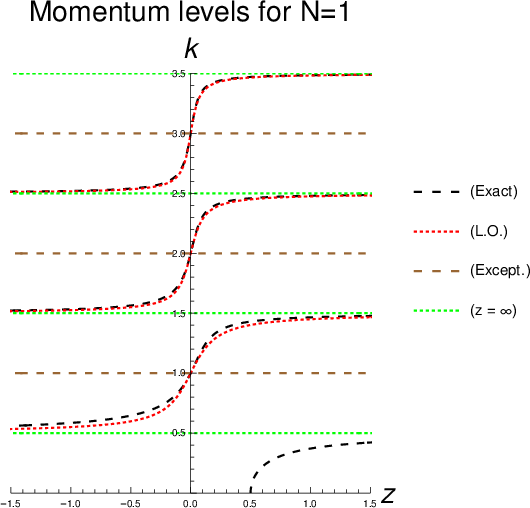
All these phenomena can be directly observed by plotting the momentum levels for a given value of the principal index and for different values of the sub-index around zero, as functions of the coupling . In fig. 1 we have taken, as an example, and we have plot the first resonant level (), together with a bunch of close non-resonant levels close, , , , .
Let us note that the non-resonant levels far from any resonant level, i.e. with large ,
| (157) |
such as, let’s say , where is the integer part of , do not exhibit a resonance behavior in any coupling region. They never resonate. These levels, as functions of , do not present two approximately flat regions connected by a linear region, as we have seen in all the previous cases (), but a smooth and slow increase in a large coupling region (see fig. 1). These properties are in agreement with simple physical intuition: momentum levels far from any resonance (in momentum space) should be very little affected by the latter.
Let us remark that, if we cut the plot in fig. 1 with a vertical line, of equation
| (158) |
we find, in general, that all the levels are quite flat at their respective intersection points, with the exception of a single level, which is linearly rising at its intersection point. We can summarize the physics above by saying that, for any (small) fixed value of the coupling , there is one, and only one, resonant-behaving level; All the other levels are dormant.
We can also observe that all the momentum levels , for any given (and fixed) and variable , restricted to their respective resonant regions, ”link together” to form a segment of a straight line, passing through the point and , of equation:
| (159) |
We can compare the above behavior with a similar behavior in standard Winter model. In the case of the latter, if we expand in powers of the pole in the complex -plane below the real axis, associated to the -th resonance, we find:
| (160) |
At first order in , the slope of the finite-volume momentum level is:
| (161) |
while that of the infinite-volume level is
| (162) |
In the limit , the slope of the finite-volume momentum line converges to the infinite-volume one; Furthermore, finite-volume corrections are of order (i.e. rather sizable).
In standard Winter model , the properties of a given resonance can be analyzed by considering its corresponding complex pole in the momentum plane, as a function of the coupling . In the corresponding finite-volume model, the behavior of the resonant state , as function of the coupling , is studied instead by gluing together different segments from many momentum levels , with .
When the coupling is very close to a critical one (an exceptional or non-generic situation), let’s say
| (163) |
the curves of the contiguous momentum levels and , are very close to each other, producing an approximate degeneracy in the momentum spectrum of the model. Therefore the critical points constitute some sort of ”transition points” of the model, where the resonant behavior moves from one level to the next one. As already remarked, there points are naturally thought of as non-generic or exceptional values of the coupling.
An approximate resummation of the perturbative corrections enhanced at large for gives [15]:
| (164) |
The function on the r.h.s. of the above equation has simple poles at all the critical couplings , , which are its only singularities. We may say that large- resummed perturbation theory ”signals” the transition of the resonant behavior from one level to the next one, by presenting singularities at all the critical (transition) points. Note also that the singularity of the above function for is an apparent one, and its power-series expansion in up to first order, for example, gives eq.(104) — as it should. Furthermore, at the middle points of the resonating intervals of the non-resonant levels,
| (165) |
the cotangent function vanishes, so that the above expression simplifies into:
| (166) |
It is worth comparing the above equation with eq.(160): The only difference is the imaginary part of the second-order coefficient, which in eq.(166) is necessarily absent.
4.2 Phase shift
The phase shift of finite-volume Winter model, as function of the particle momentum , reads [15]:
| (167) |
As well known, in the case of a resonance, the above phase quickly crosses the value (mod ), as we cross the resonance momentum (or energy).
Since the coupling is our control variable, we expect a resonant behavior to occur in our model when:
| (168) |
Therefore, for , any momentum level in its linearly-rising region (if any), i.e. where
| (169) |
gives rise to a resonant behavior, as far as phase shift is concerned. On the contrary, any momentum level in its (approximately) flat region/regions, i.e. with
| (170) |
does not gives rise to a resonant behavior, whatever (large) value of is assumed.
To have a resonant behavior, the particle momentum also has to satisfy the equation
| (171) |
where is an integer; is the quotient and is the remainder of the euclidean division of by respectively, . As already discussed, it is natural to assume for the index the range
| (172) |

4.2.1 Non-resonant case
Let us first consider the simpler case of the non-resonant levels (). Eq.(171) for exactly coincides with eq.(102), the latter giving the condition for having a local maximum of the inside/outside amplitude ratio , namely:
| (173) |
Therefore we conclude that both signals of resonance behavior simultaneously occur in all the non-resonant levels with , i.e. they occur for the same values of the momenta
| (174) |
and therefore of the coupling
| (175) |

4.2.2 Resonant case
As far as the resonant levels are concerned, one has to explicitly consider their dependence. By replacing their first-order expansion, eq.(104), inside eq.(171), one obtains for the relation:
| (176) |
while, for , one obtains
| (177) |
Therefore, by looking at the phase shift , we obtain two different values of (opposite to each other and very small in size), for which a resonant behavior is expected to occur inside . On the other hand, by looking at the amplitude ratio , just one resonant behavior is expected to occur in , inside the window , namely at .
A possible solution to the above problem involves a careful re-consideration of the properties of the resonant level . As we know, the point is a singular point of finite-volume Winter model, because the resonant level and the exceptional level cross each other precisely at this point. The same conclusion is reached by looking at the differential equation for , which has a singularity at :
| (178) |
where
| (179) |
is the standard cosecant of the angle . It is immediate to check that the above equation is non-singular in the (simpler) repulsive case, . Furthermore, the Hamiltonian of finite-volume Winter model, eq.(2), has a simple pole at .
All the facts above imply that , for real , basically consists of two independent branches, namely its restriction to , , and its restriction to , . By means of similar considerations, one concludes that also the restrictions of the exceptional level to and to are quite natural. Let us also note that the ranges of the restrictions of the resonant level, namely and of , evaluated on the half-lines where they are defined, are both equal to . They are equal to the ranges (evaluated on the entire real line) of all the non-resonant levels , . As we have shown, the resonant eigenfunction has a resonant behavior for , as in this limit. The exceptional eigenfunction , , has instead an amplitude ratio identically equal to one for any value of , so it has neither a resonant behavior nor an anti-resonant one.
Since, as we have just shown in different ways, the point is a singular point of the model, we are allowed to construct a new resonant level, let’s call it , by gluing the exceptional level, restricted to , to the resonant level, restricted to (compare fig. 3 with fig. 4):
| (180) |
In a similar way, we construct the level as:
| (181) |
The new level has a rising linear behavior in (and therefore a resonant behavior as far as amplitudes are concerned) in the interval
| (182) |
The level instead has a rising linear behavior in the interval
| (183) |
Let us now compare the range of all the momentum levels. The exceptional level has trivially zero range (it is constant!) while, as we have shown, the resonant level has range and the non-resonant levels , , have range . Therefore, the resonant level and the exceptional level have different ranges from each other, as well as from the non-resonant levels. On the contrary, the new levels and both have range , equal to the range of all the non-resonant levels. Furthermore, the new levels have shapes, in the plane, which are qualitatively more similar to the shapes of the non-resonant levels , , with respect to the old levels and . Because of the increased regularity (or symmetry), the new constructed levels seem therefore to be more natural than the old ones.
Let us now study the properties of the new levels. The level has an approximate degeneracy at the point with the lower non-resonant level (), while it has an exact degeneracy at the origin, , with the level as:
| (184) |
The minus level has a resonant behavior for , , let’s say inside the region
| (185) |
The level , in addition to the exact degeneracy at with the level just discussed, has an approximate degeneracy at with the next level (). The plus level has a resonant behavior for , more specifically in the region
| (186) |
As a consequence of the construction of the new levels, we may consider also the point as a critical point, with zero index:
| (187) |
With the above definition, it turns out that the critical couplings form a regular sequence of points in the -axis, with the constant spacing (a simple one-dimensional lattice):
| (188) |
Let us remark that, unlike the old levels and , which are smooth at the origin, the new levels have a cusp at this point. That also implies that the amplitude ratio of the level discontinuously jumps from to one as we cross the point from below (). Similarly, the amplitude ratio of the level discontinuously jumps from to , again as we cross the origin from below. These losses of regularity are however acceptable, because , as we have discussed, is a singular point, where a smooth behavior is not to be expected. Once we have ”accepted” the new plus and minus levels, we may think that the coupling value
| (189) |
where the phase shift quickly crosses the value (modulo ), is related to the resonant behavior of the plus resonant state . Indeed, the coupling is right at the middle of the interval (186) where, as we have seen, the plus state exhibits a resonant behavior as far as amplitudes are concerned. The coupling value
| (190) |
having similar properties to , is at the middle of the interval (185), where the minus state exhibits a resonant behavior as far as amplitudes are concerned.
We may conclude the present discussion by saying that, by introducing the plus and minus states in place of the resonance and exceptional states, it is possible to completely reconcile the resonance properties coming from the amplitude analysis with the resonance properties coming from phase analysis.
5 The Symmetric Case
In this section we consider Winter model at finite volume in the case , in which the two resonant cavities have the same length [25]. Because of that, the two cavities have the same resonant momenta. In other words, there are no non-resonant momenta in this case, but only resonant and exceptional momenta (see fig. 5).
Eq.(44) for the normal momentum spectrum of the model simplifies, in the case , to the transcendental equation
| (191) |
where we have defined the quantities:
| (192) |
The factor in front of the coupling , as well as the factor in front of , are purely conventional; They are inserted just to simplify the forthcoming formulae.
5.1 Resummed perturbation theory for high-energy states
The ordinary perturbative expansion for the -re-scaled momenta of the particle reads:
| (193) |
where, to simplify the formula, we have defined the re-scaled index
| (194) |
Let us consider eigenfunctions of the Hamiltonian operator of the model (eq.(2) with ) with a high energy , i.e. let us restrict ourselves to the case
| (195) |
The third-order coefficient (i.e. the term multiplied by ) on the r.h.s. of eq.(193) contains the term , proportional to , as well as the term , down by two powers of . In the above, large- region, this coefficient is clearly dominated by the first term, so that we may write, to a first approximation:
| (196) |
In general, we find that the leading terms in the perturbative expansion of the particle momentum are, for , of the form:
| (197) |
These are the terms which, for any given power of the coupling , contain the leading power of , namely . Because of the occurrence of the above ”secular terms” at high energy, we expect ordinary perturbation theory to be convergent only for:
| (198) |
i.e. only for:
| (199) |
Even in the (lucky) case in which the perturbative series has a non-zero radius of convergence , the latter is expected to vanish, according to the above relation, as for . Therefore is expected to be very small for large , i.e. for high-energy states.
The crucial point is that relation (199) implies a very strong limitation on the range of ordinary perturbation theory — an additional and stronger limitation with respect to the usual weak-coupling condition
| (200) |
If we take for example , we have to assume that:
| (201) |
while we would like to use perturbation theory for couplings much smaller than one, but much larger than the above ones, such as for example:
| (202) |
or even:
| (203) |
The conclusion of this analysis is simply that ordinary perturbation theory is not the right approximation scheme for studying high-energy states of the model. Our aim is to construct a new perturbative scheme, which still assumes weak coupling (which is, by the way, the only coupling domain relevant to resonances), but in which the quantity is not restricted anymore to be smaller than one. In other words, we are interested to the dynamical situation in which:
| (204) |
Formally, that means to consider the combined/correlated limit
| (205) |
where the constant is assumed to be different from zero (and infinity). A similar limit has been considered in ref.[26] to compute the poles of standard resonances in various -shell models.
We have already said that the maximal power of in the coefficient of is just , i.e. the maximal power of the index is equal to the current power of the coupling . In general, the coefficient of each power of is a polynomial in of degree :
| (206) |
where the ’s are real coefficients independent of and assumed to be of order one (some of them may actually vanish). In the high-energy scheme we are constructing, the above term is approximated, in Leading Order (L.O.), as we have seen, by the leading power of :
| (207) |
where, on the last member, we have introduced the new variable , defined in eq.(205). Therefore, the expansion of the particle momentum reads at the L.O. of the new perturbative scheme (205):
| (208) |
Note that the variable plays the role of an effective, state-dependent coupling of the model. Let us also remark that, since the quantity is not assumed to be small, we are not allowed to truncate the above series to any finite order in : Terms of all orders in have to be consistently included in the new perturbative scheme.
Let us observe that, in the new scheme, the expansion of at L.O. involves an infinite series of terms of the form while, in ordinary perturbation theory, the lowest-order approximation involves the term proportional to only, namely
| (209) |
By expressing for example the index in terms of and ,
| (210) |
the term , occurring in the expansion of at order in , is rewritten:
| (211) |
Since by assumption , at the Next-to-Leading Order (N.L.O.), we include, in the perturbative expansion of , all the terms in which one power of is replaced by one power of , i.e. we include all the terms of the form
| (212) |
Note that, in the new scheme, an eventual term proportional to with a coefficient independent of , is a N.L.O. one.
The new expansion of the particle momentum can be written, at N.L.O., in the form:
| (213) |
where we have defined the above functions of as the following power series in :
| (214) |
and
| (215) |
Now, at this point of the discussion, it should be clear to the reader how to construct the next-order approximation in the new scheme; It should also be clear how the general scheme works. The momentum of the particle in a high-energy state, i.e. with the index , is written as the formal sum of a function series of the form:
| (216) | |||||
From a mathematical point of view, the construction of the new perturbative scheme is legitimate, only if we can rearrange terms in the double series in and representing the particle momentum:
| (217) |
In the last equality we have changed index according to . Note that the internal sum (over ) at the last member of the above equation is infinite, while the internal sum at the second member is finite. As well-known in mathematics, a sufficient condition for terms rearrangement — the so-called unconditional convergence — is that the double series is absolutely convergent, a property therefore which we assume from now on.
Let us remark that, in the new scheme, even though we are resumming terms of all orders in even at the L.O., the all-order resummation of the perturbative series which we have realized, is an approximate one, as the coefficients are not evaluated exactly. That is because, in practice, we are always forced to truncate the function series above to some finite order (possibly large):
| (218) |
It is also important to stress that the resummation scheme which we have formally constructed is relevant — i.e. is useful in ”real life” — if, and only if, we are able to compute the series of the coefficients in closed analytic form for any value of the index , i.e. in symbolic form in , for some values of . If we do not possess such a knowledge, we are forced to truncate the series in , defining the functions , at some finite order in — an approximation which is not legitimate in the new scheme, as already noted.
To explicitly compute the functions ’s, we have to go back, from the ordinary (truncated) perturbative expansion of the momenta, to the exact equation determining the momentum spectrum of the model. We simply insert the function-series expansion given in eq.(216) inside the momentum spectrum equation (191), conveniently rewritten as:
| (219) |
The master equation is obtained:
In order to isolate the different orders in in the above equation, in the last member we have made a Taylor expansion of the function around the point . We expand then the last member of the above equation in powers of , up to the required order. By equating the coefficients of same powers of at the first and the last member, we obtain a sequence of equations of the form:
| (220) |
The first equation directly gives the L.O. function:
| (221) |
By substituting the above equation (in principle) in all the equations of the system (5.1) and solving the second equation with respect to the N.L.O. function , one obtains for the latter:
| (222) |
In a similar way, by substituting the above equation in the system and solving the third equation with respect to the Next-to-Next-to-Leading Order (N.N.L.O. or N2LO for brevity) function , one obtains for the latter:
| (223) |
At this point, it should be clear to the reader how to explicitly compute higher-order functions ’s, to any required order, as well as the general structure of the scheme. By means of a symbolic manipulation program (and a computer, of course!), the explicit evaluation of large number of functions ’s is trivial and immediate. Actually, with enough computing resources, one can evaluate an arbitrarily large number of such functions. By computing the first twenty functions by means of the Mathematica system on a standard PC, we obtained analytic approximations of the particle momentum with a relative error of order .
5.2 Comparison of resummed perturbation theory with ordinary one
In this section we compare our resummed formulae with ordinary perturbation theory ones; That provides a consistency check of the resummation scheme which we have constructed in the previous section.
According to eqs.(62) with , the momentum of the particle has the following ordinary perturbative expansion:
| (224) |
By means of a Taylor expansion of the arctangent function at the origin,
| (225) |
the expansion of the L.O. resummed formula for in powers of (eq.(218) with ), up to fifth order included, reads:
| (226) |
By comparing the last member of the above equation with the r.h.s. of eq.(224), we find that:
- 1.
The first-order term in , namely , is correctly reproduced (as it should) by the L.O. resummed formula (let us remark that any good resummation scheme should reproduce, at least, the lowest-order correction);
- 2.
The second-order term, , is totally missing in the resummed formula (the last member of eq.(226)). However, that is consistent, because this term is a N.L.O. correction, having an additional power of with respect to . Formally, the absence of this term may be seen as a trivial consequence of the fact that is an odd function of , so that only odd powers of enter the expansion of the L.O. resummed formula;
- 3.
Only the contribution of the third-order term is reproduced, while the remaining contribution, , is missing. That is (again) consistent, because the latter term is a N.N.L.O. correction, having two additional powers of with respect to ;
- 4.
The fourth-order term is completely missing in the L.O. resummed formula for the same reason of the second-order term;
- 5.
Only the contribution to the fifth-order term is reproduced by the L.O. resummed formula. The terms and are missing, as they are N2LO and N4LO corrections respectively.
We may conclude that, up to fifth order in included, our L.O. resummed formula (226) contains all the L.O. terms, i.e. all the terms of the form , .
To convince ourselves that our resummed scheme also works at higher orders, let us explicitly consider also the N.L.O. resummed formula. The expansion in powers of of the latter reads:
| (227) | |||||
By comparing the expansion in powers of of the N.L.O. resummed formula (the last line above) with the ordinary perturbative formula, the r.h.s. of eq.(224), we find that:
- 1.
The first-order term in , namely , is correctly reproduced in N.L.O. resummation, as was already the case with L.O. resummation;
- 2.
The second-order term, , is also correctly reproduced in N.L.O. resummation, as it should, such term being a N.L.O. correction. Note that this term was instead completely missing in the L.O. resummation. We see therefore a first improvement by going from L.O. to N.L.O. resummation;
- 3.
Only the contribution of the third-order term is reproduced, while the remaining contribution, , is missing, as it is a N.N.L.O. term. Therefore there is no improvement, at this order in , of the N.L.O. resummation with respect to the L.O. one;
- 4.
At fourth order, only the N.L.O. term is reproduced, while the N3LO term is missing. Note that the fourth-order term, as well as all the even-order terms, was instead completely missing in L.O. resummation;
- 5.
At fifth order, only the L.O. term is reproduced, while the N2LO term and the N4LO term are missing. Therefore, at there is no improvement with respect to LO resummation.
The above comparison of perturbative corrections for the particle momenta explicitly shows that the resummation scheme we have constructed, also works at N.L.O.. Even though we do not provide a formal proof, it is quite natural to conjecture that this scheme also works at higher orders.

5.3 Resummation of the perturbative series by recursion
In this section we present a different resummation scheme for the perturbative series of particle momenta, which is based on a sequence of functions defined recursively. As we are going to show, the two resummation schemes give the same results in Leading Order (L.O.) and begin to differ from Next-to-Leading Order (N.L.O.) on.
The idea behind the representation of the particle momentum which we are going to derive, is the following. Suppose that the variable on the r.h.s of the momentum equation (191), namely
| (228) |
is replaced by some constant, let’s call it (which is non zero but is, for the moment, arbitrary). The above equation then simplifies to the equation
| (229) |
which can be immediately solved to give:
| (230) |
The function is the branch of the multi-valued arctangent function, having image, for a real argument , in the interval :33 3 As function of a complex argument (complex function), is a multi-valued analytic function, with logarithmic branch points at . To make single-valued, i.e. to obtain well-defined analytic branches, we can cut the complex plane, for example, along the imaginary axis, from to and from from to . By writing , , the above cuts have equations Since these cuts do not cross the real axis of the -plane, i.e. the -axis, the branches of so constructed are continuous for real .
| (231) |
Sometimes, to stress such choice, we will denote this branch by .
We can reduce ourselves to the above ”desirable” situation () by means of the following reasoning. Eq.(228) involves a periodic function, namely , of period (which is a quantity of order one), and a monotonic function, . Inside any period , , such as for example the fundamental period (corresponding to the choice ), the function takes all its values, ranging from to . Let’s now think to as an independent variable. If we consider a large starting value of this variable,
| (232) |
and make an increment of the latter of order one (or of order , if preferred),
| (233) |
the relative (or fractional) change of the function will be small as, by definition,
| (234) |
while the relative change of the function will be, in general, very large. Now, eq.(191) can be trivially rewritten as:
| (235) |
In the weak-coupling regime,
| (236) |
we can consider the situation in which:44 4 In ordinary (or straightforward) perturbation theory, one assumes instead that , while .
| (237) |
so that:
| (238) |
while, generically:
| (239) |
Therefore let us consider a high-energy expansion for the particle momentum of the form:
| (240) |
where we have defined the convenient index
| (241) |
The index is assumed to be large, while is assumed to be a generic quantity of order one (as will be checked a posteriori):
| (242) |
Since the modulus of their ratio is small,
| (243) |
the quantity
| (244) |
provides us the required expansion parameter. By substituting the expansion for given in eq.(240) inside eq.(228), one obtains:
| (245) |
where we have explicitly taken into account the periodicity of , so that:
| (246) |
The crucial point is that the first member of eq.(245) only depends on the correction term , as the leading term has disappeared. Instead, the last member of eq.(245) depends on both and , which however are both multiplied by the small coupling . The idea now is to analyze the size of the various terms which enter the first and the last member of eq.(245), namely the basic equation
| (247) |
It is easily found that is the smallest quantity entering eq.(247) because:
- 1.
It is much smaller than the momentum correction term , appearing on the r.h.s. of eq.(247), because it is multiplied by the small coupling :
(248) - 2.
It is much smaller than the quantity ,
(249) because, by assumption:
(250)
Therefore, to a first approximation, one can safely neglect the term in eq.(247), obtaining the much simpler equation
| (251) |
The latter equation can be immediately solved to give:
| (252) |
Note that the result obtained, the last member of eq.(252), is not trivial at all, and does not coincide with the corresponding ordinary perturbation expression previously obtained. Note also that, as anticipated at the beginning of this section, eq.(252) exactly coincides with the L.O. resummed momentum derived in the previous section (involving the function only), given in eq.(221).
Arrived at this point, we can also check the correctness of our initial small-parameter assumption . For any real argument , the uniform bound holds
| (253) |
It follows that:
| (254) |
Now, to evaluate sub-leading corrections to in this scheme and, in general, to derive a systematic expansion, the idea is simply to think to the above, leading approximation, as the first step of a recursion process. Therefore let’s go back to the exact momentum equation (247). By thinking to the small term as a known quantity, we can formally solve eq.(247) with respect to the momentum correction term appearing at its l.h.s.:
| (255) |
We solve the above equation recursively in the following way. We generate a sequence of functions
| (256) |
by means of the following one-step recursion equation:
| (257) |
The initial condition is given at and coincides with the free limit , i.e. a vanishing value of the momentum correction :
| (258) |
Therefore the momentum shift is the fixed point of the map given in eq.(257). The momentum level is given by the limit of the above function sequence:
| (259) |
We have checked numerically the convergence of the function series to in many cases (see fig. 6), which turns out to be quite fast with the recursion order and uniform in . We admit that we do not have an analytic proof of the convergence yet, which is, in any case, well beyond the aims of the present paper.
There is an equivalent formulation of the recursive solution for , involving the complete momentum of the particle in place of the momentum correction . One constructs the sequence of functions
| (260) |
by means of the following recursion equation:
| (261) |
The initial condition reads:
| (262) |
The complete particle momentum (including the -th order term ) is simply the limit of the above sequence:
| (263) |
Let us work out explicitly the first few recursions, in the first scheme constructed. At the lowest, zero order:
| (264) |
so that:
| (265) |
The zero order is, by definition, trivial. The first recursion gives:
| (266) |
The function on the last member of the above equation exactly coincides with the approximation to the particle momentum obtained in eq.(252). Therefore, with the first recursion, we obtain the lowest-order non-trivial approximation to the particle momentum.
The second recursion reads:
| (267) |
In a similar way, the third recursion is written:
| (268) |
We may notice that a recursion step is obtained, in general, by substituting in the ”innermost place” with :
| (269) |
We may also notice that the above rule is obtained by multiplying, on both sides by the coupling , the basic replacement rule
| (270) |
which represents the first recursion step (, compare eq.(265) with eq.(266)). The observation leading to the substitution rule (269) can be formalized in the following way. Let us define the function
| (271) |
Note that , i.e. depends on both and parametrically. In terms of the function , the second recursion can be written:
| (272) |
and the third recursion:
| (273) |
In general, by iterating the recursion, one evaluates the composition of with itself a progressively larger number of times. Therefore let us define as the composition of with itself times:
| (274) |
i.e.:
| (275) |
For example, by taking , we obtain the function
| (276) |
meaning, as well known, that:
| (277) |
It is natural to define and (i.e. is simply the initial function , while is the identity function). In terms of the sequence of functions , the -th recursion for the momentum can be written in the following compact way:
| (278) |
Let us end this section by noting that the momentum level , obtained as the limit of for , contains, roughly speaking, an infinite number of compositions of the function with itself.

5.4 Comparison between the two resummation schemes
In the previous sections, we presented two different (both approximate) resummation schemes for the perturbative series of the particle momenta. As we have discussed in detail, the first scheme is based on a (truncated) function series, while the second scheme is based on the approximate (i.e. finite order) solution of a recursion equation. It is quite natural, arrived at this point, to compare the two schemes, in order to find their common properties, as well as their differences. That is indeed the aim of the present section.
As already discussed, in the recursive scheme, the first recursion,
| (279) |
exactly coincides with the function series truncated at first order, which we have called the Leading Order (L.O.) approximation ( in eq.(218)):
| (280) |
The leading-order agreement is related to the fact that it turns out that:
| (281) |
At second order, i.e. at N.L.O., the two schemes begin to (slightly) differ from each other (see fig. 7). The scheme based on the function series gives, at N.L.O.:
| (282) |
The scheme based on the recursion equation gives instead, for the second recursion, as we have seen:
| (283) |
Note that the latter formula, unlike the previous one, contains terms of all orders in . By expanding the r.h.s. of the above equation in powers of up to second order, one obtains:
| (284) |
The second-order term in on the r.h.s. of the above equation is naturally compared with the N.N.L.O. function which, according to eq.(223), is given by:
| (285) |
By comparing the last member of eq.(282) with the r.h.s. of eq.(284), one finds that the second recursion contains the first contribution to , namely the term
| (286) |
Note that the above term is the dominant one in for , because of the additional factor at the numerator. By pushing the expansion of in powers of to even higher orders, one finds that the second recursion also contains the leading contributions to , , , , for . With a suggestive language, we may say that the scheme based on the recursion equation ”resums the resummation” realized by the function-series scheme. Such a ”resummation of a resummation” is, of course, again an approximate one (we are not able to solve exactly the momentum-spectrum equation!) and is relevant in the case .
Let us also note that the functions and can also be computed, in addition to the direct evaluation described at the end of sec. 5.1, also by expanding the second recursion in powers of up to first order. In general, the functions
| (287) |
can be computed by expanding , the recursion of order , in powers of up to the order included.
A natural question at this point is which resummation scheme, among the two, is preferable. It is fair to say that each scheme has its own virtues and shortcomings. The scheme based on the function series — let’s call it the first scheme — is conceptually simpler, as it involves truncated expansions in the small parameter . The scheme based on the recursion equation — let’s call it the second scheme — includes higher-order terms in , which are missed in a truncated power series in , and which are the dominant ones for very large . In view of this latter fact, we may conclude that the second resummation scheme is perhaps better than the first one in the intermediate and in the large coupling regions (), or in the description of states with very high energies. Because of that, in the following sections we will mostly consider the second or recursive scheme.
5.5 Discussion
Finite-volume Winter model in the symmetric case , in which the two resonant cavities have the same length, is an oscillating, rather than a decaying system. Amplitude is constantly transferred from one cavity to the other, back and forth. Similar oscillation phenomena occur in classical mechanics, by considering for example two weakly-coupled harmonic oscillators, where energy is constantly transferred from one mode to the other [27].
To fully understand the dynamics of the model, we may consider the explicit time evolution of a wavefunction initially contained in the ”small” cavity , i.e. identically vanishing in the ”large” cavity , which is equal to a box eigenfunction:
| (288) |
where is a positive integer and for and zero otherwise is the usual Heaviside step function. Since the two cavities have the same length or, equivalently, because of the absence of non-resonant levels, we expect the no-escape probability, for example,
| (289) |
to not exhibit an approximate exponential decay in any time region. Heuristically, we may consider the exponential decay of an unstable state with time a statistical phenomenon, in which the initial amplitude, contained in the small cavity, is transferred to the large number of available states of the system. Since the large cavity has the same density of states (in momentum space) of the small one, the former is not expected to be able to ”exponentially absorb”, for some time, a large part of the initial amplitude.
We may conclude that the symmetric case is qualitatively different from the quasi-continuum one () and describes oscillation, rather than decay, phenomena.
6 The Double Case
In this section we consider Winter model at finite volume in the particular case , in which the right cavity (the large one) is two times larger than the left one (the small one).
In this case, resonant levels , having integer limit in the free limit, alternate with non-resonant levels , having instead semi-integer limit for . In other words, resonant levels and non-resonant ones separate each other (see fig. 8). The equation for the normal part of the momentum spectrum explicitly reads:
| (290) |
where:
| (291) |
Note that eq.(290) is considerably more complex than eq.(191), the latter describing the physically and mathematically much simpler case.
Now it comes one of the main technical ideas of this work, which will be used also in the larger cases: we transform , the tangent of the double momentum above, into a rational function (of degree two) in , the tangent of the momentum . The general tangent reduction formula is derived in Appendix A, which, in the case , reduces to the first of eqs.(A). By means of the latter, a non-linearity of transcendental type is converted into a non-linearity of algebraic type, which is much more tractable. By means of the first of eqs.(A), the momentum equation above is rewritten:
| (292) |
By assuming to be a known quantity, we can solve the above equation with respect to , obtaining:
| (293) |
The two sign determinations in front of the arithmetic (i.e. positive) square root above give rise to two different sequence of levels. Indeed, in the weak-coupling regime, , the plus/minus equations read respectively:
| (294) | |||||
| (295) |
In the first case 1., by taking the free limit , the function vanishes, implying that tends to an integer , times . Therefore the ”plus equation” above describes the resonant levels of the system.
In the second case 2., for , instead diverges, so that tends to , i.e. to a half-integer, times . Therefore the ”minus equation” above describes the non-resonant levels.
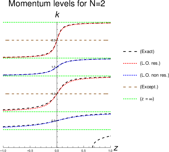
6.1 Resonant levels
Let us first consider the simpler, resonant case 1. The particle momentum is naturally decomposed, as in the previous case, as:
| (296) |
where:
| (297) |
Eq.(294) is then rewritten:
| (298) |
Just as in the case , there are two possible resummation schemes for the perturbative series of the particle momenta, which are discussed separately in the next sections.
6.1.1 Resummation by means of a function series
The perturbative series for the resonant particle momentum can be (approximately) resummed to all orders in
| (299) |
and to finite order in , by means of a function series. Similarly to the previous case, the particle momentum is written:
| (300) |
where the non-negative integer specifies the order of the approximation. The Leading-Order (L.O.) function (corresponding to the choice ) and the Next-to-Leading Order (N.L.O.) function () have the following explicit expressions:
| (301) |
The evaluation of higher-order functions is, in principle, straightforward. However, by increasing , i.e. the order of the approximation, the complexity of the functions grows quite quickly.
6.1.2 Resummation by recursion
Similarly to the previous case, the momentum of the particle is written:
| (302) |
According to the above decomposition, eq.(294) is conveniently rewritten:
| (303) |
We construct a function sequence by means of the following one-step recursion in the index :
| (304) |
with the initial condition (at ):
| (305) |
The function is obtained as the limit of the above function sequence:
| (306) |
In practice, it is sufficient to compute few recursions only, as they already provide a good, uniform approximation in , to the exact result. In other words, convergence of the function sequence to the exact momentum level (for ) is rather fast.
The first recursion () gives the lowest-order non-trivial approximation for the resonant particle momenta and explicitly reads:
| (307) |
Let us remark that it is not legitimate to expand the square root above in powers of , as is not, by assumption, a small variable.
By means of eq.(304) for , the second recursion is written:
| (308) |
with explicitly given in the previous equation (307). To give the reader an idea about the kind of functions coming out of the recursions, let us give the second recursion for in completely explicitly form:
| (309) |
Similarly to the previous case, we may notice that a recursion step is obtained by replacing , in its innermost place, according to the rule:
| (310) |
The above rule, in turn, is obtained by multiplying on both sides by , the basic substitution rule
| (311) |
The recursions are easily written by means of the function
| (312) |
The treatment is similar to the case, so we omit the details. The resonant momentum at the step is written:
| (313) |
where is the (function) composition of with itself times, with and .
6.1.3 Comparison with ordinary perturbation theory
The comparison of the perturbative resummed formulae derived in the above two sections with the fixed-order ones is completely similar to the case, so we just sketch the procedure; The actual computation is left to the reader as an exercise. We expand in powers of eq.(300), with a selected value of , or eq.(304), with a selected value of . We then compare the coefficients of the various powers of with the coefficients given in eqs.(62), in which we have set .
6.2 Non-resonant levels
In this section we consider the non-resonant levels of the system, described by eq.(295) (the case ). For the weak-coupling expansion, , it is convenient to write the particle momentum in the form
| (314) |
where we have defined the ”ad-hoc” index, involving semi-integer numbers,
| (315) |
Note that:
| (316) |
and that vanishes in the free limit:
| (317) |
By means of the formula
| (318) |
the following equation for the non-resonant momentum shift is obtained from eq.(295):
| (319) |
The above equation can also be obtained by transforming eq.(295) according to the formula
| (320) |
We consider the simpler repulsive case , implying (the attractive case, , is obtained later, from the case , by means of analytic continuation; That way, continuity of particle momenta at is guaranteed).
The complete particle momentum , according to eq.(314), satisfies the following equation:
| (321) |
Note that the above equation is still exact and that the only differences with respect to the corresponding resonance equation (296) are:
- 1.
In the lowest-order term (coinciding with the free limit ), the index is replaced by the new index , the latter containing an additional, half-integer contribution;
- 2.
The argument of the arctangent function contains an additional factor three at the denominator. That implies, in particular, that, in the weak-coupling region, the growth of the non-resonant momentum with is softer with respect to the resonant case.
Just like in the resonant case, also in the non-resonant case two resummation schemes are available, which are discussed in the next sections.
6.2.1 Resummation by function series
The non-resonant particle momentum is written as the following function series:
| (322) |
where specifies the order of the approximation and we have defined the convenient -type variable
| (323) |
The evaluation of the functions is straightforward. For concreteness sake, let’s just give explicitly the L.O. function:
| (324) |
6.2.2 Resummation by recursion
Similarly to the previous cases, a function sequence converging to the desired function is generated by means of the following recursion equation:
| (325) |
with
| (326) |
The initial condition, as usual, coincides with the free limit of the non-resonant levels:
| (327) |
The first recursion () provides the lowest-order, non-trivial approximation for the non-resonant momenta:
| (328) |
Note that the correction term in the above equation, i.e. the second term at its r.h.s., exactly coincides with the L.O. function given in eq.(324). Therefore the two resummation schemes exactly coincide, at the first non-trivial order, also in this case. Note also that the first-order momentum correction
| (329) |
is an odd function of . The second recursion () is written in terms of the first one () as:
| (330) |
As observed before by looking at the exact equation, because of the factor three at the denominator of the argument of the arctangent function at the r.h.s. of eq.(328) and (330), the growth of the particle momentum with the coupling is softer in the non-resonant case with respect to the resonant one. This observation [15] has also been made in section 4 on the basis of ordinary perturbation-theory formulae. This factor three is also responsable of the smaller range of the non-resonant levels (by a factor two) with respect to the resonant ones (see fig. 8).
6.2.3 Comparison with ordinary perturbation theory
Since the resummation of the perturbative series of a non-resonant momentum — eq.(328) for the first order and eq.(330) for the second order in the recursive scheme — constitutes a new kind of resummation, let us discuss in this section, in some detail, the comparison with ordinary perturbation-theory formulae.
By evaluating the coefficients of ordinary perturbation theory — eqs.(78) for —, one obtains, up to third order in included:
| (331) |
The expansion in powers of of the first recursion, eq.(328), reads instead:
| (332) |
As in previous cases, the first recursion correctly reproduces the first-order term in , completely misses the second-order term and gives only the leading, large- contribution at third order.
6.3 Discussion
Finite-volume Winter model in the double case, , in which the large cavity, , is two times larger than the small one, , is, in a sense, the lowest- non-trivial case. Even though cannot be reasonably considered a large number, by going from the case to the case , we begin to see, in the small-coupling domain , some hints of resonance dynamics of the quasi-continuum . The density of states of the large cavity (in momentum space) is indeed two times larger than that of the small cavity, so that non-resonant levels occur in the spectrum.
We may say that the main change, by going from to , is indeed the appearance of non-resonant levels in the momentum spectrum of the model. The latter are rather symmetrical under a change of sign of the coupling, i.e. for , so they cannot be naturally associated to the contiguous upper or lower resonant level. As already noted, the L.O. approximation to the momentum shift , eq.(329), is indeed an odd function of the coupling . Furthermore, as we have shown again with analytic computations, non-resonant levels have a smaller slope around than resonant ones. Unlike what happens in the quasi-continuum case (see sec.4), non-resonant levels do not exhibit a resonant behavior in any coupling region. The main role of non-resonant levels is simply that of separating the resonant levels from each other.
7 General method
The transcendental equation (44) for the ordinary momentum spectrum of the model can be written:
| (333) |
By using the tangent reduction equation (522), derived in Appendix A, inside the momentum equation above, one obtains an equation of the form:
| (334) |
where:
| (335) |
To simplify notation, we have defined
| (336) |
In the last equality above we have used eq.(523) in Appendix A. The explicit expressions of the polynomials and are given by eqs.(524) and (525) respectively. For even , the numerator of the rational function (in ) on the last member of eq.(335) has degree , while the denominator has degree . For odd , the degrees are reverted: The numerator has degree , while the denominator has degree . Therefore, for any , also is a rational function of degree in its argument , like .
Eq.(334) can be rewritten as a general polynomial equation in of order , with coefficients dependent on (the latter quantity is assumed to be known):
| (337) |
All the coefficients of are real for , i.e. for a real coupling (the physical case). It is immediate to check that, for any , the polynomial has degree . For , i.e. in practice in the cases (the case is, of course, trivial), the above equation can be explicitly solved with respect to in terms of nested radicals — involving square roots and cubic roots — and rational operations. For , because of Galois theory, it is instead in general impossible to solve the above equation in terms of radicals; In the latter case, one is forced to use special functions. That makes the cases , in practice, much less elementary and tractable than the ones.
Because of the fundamental theorem of algebra, the above equation, namely
| (338) |
has in general solutions, usually called zeroes or roots, , for any specified value of the coefficients . By varying , the zeroes, , , , , also vary, so that we may think that the above equation implicitly defines a multi-valued function . Let us choose one branch among its branches, , let’s say , so that:
| (339) |
Formally, we may write:
| (340) |
For , the branches , originate from properly cutting the complex planes where the square roots and cubic roots of the formulae for the zeroes, are defined.
Eq.(339) can also be derived by taking the formal inverse of on both sides of eq.(334), i.e. by applying the function to both sides of this equation. Since, in general, the function is not one-to-one, the inverse function is multi-valued. Generally, is a map, i.e. , in general distinct, ’s have the same image under . That implies that has different branches, corresponding to the non-resonant levels for each resonant (and exceptional) level. The branch of , which we have selected, is fixed from now on.
7.1 Resummation by recursion
Now it comes the fundamental decomposition of the particle momentum , which allows substantial simplifications due to the periodicity of the tangent:
| (341) |
where:
| (342) |
By taking indeed into account the periodicity of the tangent, eq.(339) is transformed into the equation
| (343) |
where we have defined the effective coupling
| (344) |
Note that eq.(343) does not explicitly depend on which, as we are going to show later in this section, is the largest quantity in the problem.
By taking the formal inverse of the tangent on both sides of eq.(343), i.e. by applying the arctangent function on both sides, one obtains the equation:
| (345) |
where we have defined the function
| (346) |
To obtain a well-defined equation, one has to select an (arbitrary) branch of the arctangent function. We have assumed the branch with image, for a real argument, in the interval , which we have denoted , and which is also fixed from now on. Note that we have already implicitly taken into account the multi-valued character of the arctangent function by writing in the form (341) and also by going from eq.(339) to eq.(343). To simplify the notation, let us drop both indices and in , so that, from now on, .
Let us observe that, in the momentum levels , the principal index is related to the infinite multivaluedness of the general arctangent function, while the sub-index is related to the finite multivaluedness, ”-valuedness”, of the function .
According to eq.(341), the total momentum of the particle is written:
| (347) |
Let us now assume to be at high energies, i.e. at high momenta:
| (348) |
or, equivalently:
| (349) |
as well as in the weak-coupling regime:
| (350) |
We also assume that , the product of the above variables and , is of order one, or somewhat larger than one:
| (351) |
In the above region, if the function vanishes at the origin, i.e.
| (352) |
as it happens for the resonant levels, it makes sense to construct the following recursion equation out of eq.(345):
| (353) |
with the initial condition (at ):
| (354) |
We had to assume , because the initial condition, accompanying the recursion equation in , assigns to the initial momentum shift , at , its free-theory value (). If the function does not vanish at the origin, as it happens for the non-resonant levels, we redefine by subtracting its value in zero:
| (355) |
Eq.(347) for the particle momentum is then rewritten:
| (356) |
where:
| (357) |
and
| (358) |
Let us look at the first few recursions (we do not write the tilde’s, but we consider both cases and ). The first recursion gives:
| (359) |
where, on the last member, we have imposed the vanishing initial condition, eq.(354).
If we consider the total particle momentum , we see that the first recursion simply adds to the free-theory momentum :
| (360) |
Therefore the first recursion is equivalent to the following replacement rule:
| (361) |
Let’s now consider the second recursion, which is given by:
| (362) |
where, on the last member, we have replaced the first recursion, i.e. we have used eq.(359). Therefore, going from the first recursion to the second one involves the ”transition”
| (363) |
The second recursion step () is then equivalent to the following substitution inside the argument of the function :
| (364) |
Note that the above rule (364) simply comes from multiplying by on both sides the basic replacement rule (361).
In order to understand the functional character of the general recursion equation above, let us define the function
| (365) |
It is immediate to check that the second recursion can be written in terms of evaluated at the point , as:
| (366) |
In order to find some general rules in the recursions, i.e. some mathematical structures produced by the repeated recursions — if any —, let us work out the third recursion:
| (367) |
Therefore, with the third recursion step , , the momentum shift from the free value, is modified as:
| (368) |
We may notice that, in the expression for above on the left, the variable occurs two times, namely inside the argument of the external function ,
| (369) |
and as the argument of the internal function,
| (370) |
By going from the second recursion to the third one, one may note that the first occurrence of on the left of (368) (see eq.(369)) is not modified. In the second occurrence, (see eq.(370)), the variable is instead transformed according to rule (364), which we have already used in going from to . In other words, by going from the second recursion to the third one, the variable is replaced according to the rule (364) only in the innermost place.
In terms of the function defined in eq.(365), it is easy to check that the third recursion can be written:
| (371) |
The composition of with itself, evaluated at the point , is the argument of .
We may generalize the above observations by conjecturing that any recursion step () is obtained by shifting according to the rule (364) in the innermost place, i.e. inside the innermost function . By explicitly looking at higher order recursions, we find that the above conjecture is true, namely:
| (372) |
Furthermore, the momentum correction can be written, in general, in terms of the function as:
| (373) |
where is the composition of the function with itself times. By convention,
| (374) |
By defining the zero-index function as the identity function,
| (375) |
one may write also the first recursion using the general formula (373):
| (376) |
7.2 Resummation by function series
The perturbative series for the particle momentum can also be (approximately) resummed to all orders in , by means of a (truncated) series of functions of multiplied by progressively higher powers of :
| (377) |
In general, by expanding , i.e. the solution of order of the recursive equation, in powers of up to order included, and comparing with the r.h.s. of the above equation, one obtains the following expression for the ’s:
| (378) |
Note that the variables and are independent from each other. By considering, for example, the third-order recursive solution given in eq.(367), we obtain for the first three functions, according to the above equation (with ):
| (379) | |||||
8 The Triple Case
In this section we consider Winter model at finite volume in the case , in which the right cavity (the large one) is three times larger than the left one (the small one). As we are going to show, this case can be reasonably considered a ”large-” case.
In the free limit , the momenta of the particle become integer multiples of :
| (380) |
Therefore there are two contiguous non-resonant levels before (or after) each resonant (or exceptional) level (see fig. 9).
The equation for the -rescaled momenta of the particle is simply obtained by setting in the general momentum equation (44):
| (381) |
By expressing the function as a rational function (of third order) in , as shown in appendix A, the above equation can be transformed into the equation:
| (382) |
In the free limit , if the above equation is to be satisfied, one of the factors at the numerator of the rational function in at its l.h.s., has to vanish. There are three different possibilities:
| (383) |
We have taken into account that, with our choice of the arctangent branch, . In the first case , we find the sequence of the resonant levels, while in the second case and in the third one , we find the two sequences of non-resonant levels.
The momentum equation (382) can be trivially transformed into the following algebraic equation:
| (384) |
where, to make the formulas more compact, we have defined:
| (385) |
We have also introduced the convenient variable:
| (386) |
involving the effective coupling
| (387) |
In terms of the coupling :
| (388) |
Note that eq.(384) is a general, third-order algebraic equation in with real coefficients. By means of standard Cardano’s formula for third-order algebraic equations (see Appendix B), the explicit solutions of the above equation for can be written:
| (389) |
where:
| (390) |
and we have defined the (nested) radicals:
| (391) |
with:
| (392) |
Note that the index is defined modulo three, so we can limit ourselves, for example, to consider the values:
| (393) |
Note also that, with our branch of the cubic root:
| (394) |
where a bar above a quantity denotes its complex conjugation. Different multi-valued functions do appear in eq.(389) so, in order to avoid ambiguities, let us specify in detail their branches:
- 1.
The square root in the function is the arithmetical (i.e. positive) one: . That is consistent because, for any real value of (the physical case), the argument of the above square root is always positive (actually, it is greater than one). In general, we consider the following branch of the complex square root. By writing a (non-zero) complex number in the polar form
(395) our square-root branch is defined by:
(396) - 2.
The choice of the branch of the cubic root appearing in the definition of the functions , i.e. of the function , is similar to the one of the square root. We cut the complex -plane along the negative part of the real axis, namely for , and we select the branch which is real on the positive axis: . By writing the independent variable in polar form as in eq.(395), the cubic root branch in defined by:
(397) - 3.
We select the usual branch of the function, which is continuous and odd for real argument, vanishes at the origin, , and has image, again for real argument, in the interval .
Let us now comment on our main result, namely eq.(389). For each value of the index , the solution is real for any real value of . That is because the second and third terms inside the curly bracket on the r.h.s. of eq.(389), are complex conjugate of each other. Therefore there are always three real and distinct roots. That is in complete agreement with physics: We know that, for any choice of the integer in eq.(389), there must be three real momentum values for any value of the coupling . Note also that all the radicals we have introduced are normalized to one at , i.e. in the free limit:
| (398) |
For , the phase factors in front of the cubic roots in eq.(389)
| (399) |
i.e. they become opposite of each other. That implies that:
| (400) |
so that the index choice gives the resonant levels. The remaining index choices give the non-resonant levels, as:
| (401) |
The high-energy expansions of the resonant and non-resonant momenta are discussed in the following sections.
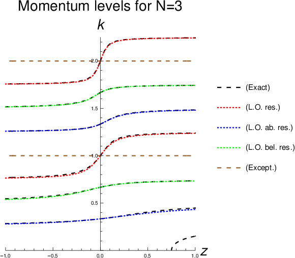
8.1 Resonant levels
By setting in the general eq.(389), one obtains the following equation for the resonant particle momenta:
| (402) |
where we have defined the function
| (403) |
The variable is the value taken by for :
| (404) |
as . Note that:
| (405) |
as it should. Similarly to previous cases, we can solve the above equation by means of a function-series expansion or by means of a recursion equation, as described in the next two sub-sections.
8.1.1 Resummation by means of a function series
The resonant levels posses a function-series expansion of the form:
| (406) |
where we have defined:
| (407) |
The Leading-Order (L.O.) function reads:
| (408) |
where the function has been defined in eq.(403). The computation of higher-order functions is straightforward and is easily made, for example, by following the general method described in section 7.2. By substituting with (as is replaced by ) in eq.(7.2), one obtains for the second-order function and the third-order one respectively:
| (409) |
8.1.2 Resummation by recursion
In the recursive scheme, the resonant particle momentum is written:
| (410) |
The momentum correction to the (large) free-theory value is obtained as the limit of a function sequence :
| (411) |
The function sequence is constructed by means of the following recursion equation:
| (412) |
with the initial condition, at :
| (413) |
The first recursion () gives for the complete momentum:
| (414) |
where the function has been defined in eq.(403). The above first-order result, which is independent, is in complete agreement with the L.O. approximation for in the function-series scheme, eq.(408). By substituting with and with in eq.(362) and (367), one obtains for the second and third recursions respectively:
| (415) |
8.2 Non-resonant levels above the resonant ones
In this section we consider the (approximate) resummation, to all orders in the coupling , of the perturbative series of the non-resonant momentum levels right above the resonance ones. These are the momentum levels with the principal index and the sub-index , of the form:
| (416) |
where we have defined the new variable
| (417) |
and the shifted index
| (418) |
As in the non-resonant case of the model previously considered, resummation is made either by means of a function series expansion or by means of a recursion equation.
8.2.1 Resummation by function series
For the non-resonant levels right above the resonant ones, i.e. with , the function-series expansion holds:
| (419) |
The Leading-Order (L.O.) function explicitly reads:
| (420) |
where we have defined the function
| (421) |
Note that is real for a real argument (the physical case) and that:
| (422) |
Higher-order functions , , are easily calculated by following the general method described in section 7.2. In the formulae in the latter section, one has to make the following replacements: , , and .
It is remarkable that the above, L.O. formula provides a fairly good approximation to the exact momentum levels also at , i.e. to (the lower blue dotted line in fig. 9).
8.2.2 Resummation by recursion
In the recursive scheme, the non-resonant particle momenta are written:
| (423) |
The non-resonant momentum correction, , is obtained as the limit of a function sequence :
| (424) |
The function sequence is constructed by means of the following recursion equation:
| (425) |
with the initial condition, at :
| (426) |
Higher-order recursions are easily computed by means of the general method described in section 7.1. One has to change the symbols in the equations of the latter section as described at the end of the previous section.
8.3 Non-resonant levels below the resonant ones
In this section we consider the resummation of the perturbative series of the non-resonant momentum levels right below the resonance ones, i.e. the levels with the sub-index :
| (427) |
where we have defined the new variable
| (428) |
and the new shifted index
| (429) |
Unlike the previous case , in this case the principal-index value has to be discarded, so that . Apart from this detail, this case closely parallels the previous one, so the discussion will be very concise.
8.3.1 Resummation by means of a function series
The resummation of the non-resonant levels below the resonant ones, i.e. with , involves a function series-expansion of the form:
| (430) |
The L.O. function explicitly reads:
| (431) |
where we have defined the function:
| (432) |
8.3.2 Resummation by recursion
In the recursive scheme, the non-resonant particle momenta with are written:
| (433) |
The non-resonant momentum correction, , is obtained as the limit of a function sequence :
| (434) |
The function sequence is constructed by means of the following recursion equation:
| (435) |
The initial condition to the non-resonant momentum shift, assigned at , is, as usual, given by the vanishing, free-theory value:
| (436) |
8.4 Limits of analytical computations
In order to analytically evaluate the momentum spectrum of finite-volume Winter model in the case , we had to solve a general, third-order algebraic equation with real coefficients, finding three real and distinct roots. In algebra, this case is called the irreducible one [28], because it is not possible to express the real roots in terms of radicals involving real numbers only. Even though the final results are all real, it is necessary to go through the complex numbers. Any momentum is written indeed as the arctangent of a real quantity plus (two times) the real part of a truly complex number (see for example eq.(402)). This situation is to be contrasted with the one encountered in the previous case , where much simpler second-order equations were involved and the real roots could be written in terms of radicals of real numbers.
Because of this mathematical irreducibility phenomenon, the formulae for the particle momenta in the case are much less readable than the formulae in the case . As we have shown in the previous sections, in the case one has to (arbitrarily but necessarily) fix branches of various multi-valued functions, so that at the end the intuitive content of the formulae is drastically reduced with respect to the case .
As we are going to show in the next section, the new mathematical situation which we have found by going from the case to the case persists — and actually gets much worse — in the case , where general algebraic equations with real coefficients of fourth order have to be solved.
8.5 Discussion
People say that in physics there is one, two, three, infinity. By that, they mean that relatively small- cases, such as the case , offer the possibility of describing some qualitative properties of the case as well as, approximately, some quantitative properties.
In the case, the density of states of the large cavity is, in momentum space, three times bigger than that of the small cavity, implying that two contiguous resonant levels, with indices and , with , are separated by a pair of non-resonant levels, with indices and . A non-resonant level, right above a resonant one, , has most of its variation at positive couplings, , where it exhibits a mild resonant behavior. Therefore, as far as resonance dynamics is concerned, a level is naturally related to this lower, contiguous resonant level . Similarly, a non-resonant level, right below a resonant one, , has most of its variation at , where it exhibits a mild resonant behavior. Therefore the level is related to the contiguous, upper resonant level, .
The conclusion is that, as far as resonance behavior is concerned, the momentum levels of the model naturally group into triplets, centered around a resonant level.
If the case can be considered a large- case, as we conjecture, an initial box eigenfunction contained in the small cavity — the analog of the wavefunction in eq.(288) — should exhibit an approximate exponential decay with time in some intermediate temporal window.
9 The Quadruple case
In this section we consider Winter model at finite volume for , in which the left cavity (the large one) is four times larger than the right one (the small one). This is the largest- case which we can treat using the fundamental algebraic simplification introduced in the case (involving the reduction of the tangent of a multiple argument), by means of elementary functions.
In the free-theory limit, , the allowed momenta of the particle tend to integer multiples of ,
| (437) |
Therefore there are three contiguous non-resonant levels for each resonant level (and exceptional level).
The equation in determining the normal part of the momentum spectrum of the model reads:
| (438) |
The denominator of the fraction on the r.h.s. of the above equation vanishes for:
| (439) |
where the numerator does not vanish (the two sign determinations in the above equation are independent from each other because a bi-quadratic equation has been solved). Furthermore, the numerator vanishes at , where the denominator does not vanish. Therefore the zeroes of the numerator on the r.h.s. of eq.(438) are zeroes of the complete expression. In the free limit , eq.(438) is satisfied in the following four cases:
| (440) |
In general, for even , i.e. for
| (441) |
there is a non-resonant momentum level with , having, for , the semi-integer limit
| (442) |
and lying therefore exactly at the middle of two consecutive resonant levels, and .
Eq.(438) is easily transformed into the following monic fourth-order algebraic equation in :
| (443) |
Note that the coupling appears in the coefficients of the above polynomial always at the denominator, making the study of the limit more difficult than in the case , where appears at the numerator (cfr. eq.(384)).
The usual decomposition of the particle momenta reads:
| (444) |
where:
| (445) |
By exactly solving the above equation in , one obtains for the function the rather involved expression:
| (446) |
The indices are two independent sign determinations. The branches of the square root, the cubic root and the arctangent function are the same as those defined in sec. 8 (the case ). The function is proportional to an (arbitrary) solution of the auxiliary third-order equation (see Appendix C); It is explicitly given by:
| (447) |
The functions involve an overall cubic root and differ from each other by a sign only:
| (448) |
The function is the inner-most radical:
| (449) |
Finally, the variable is the product of the independent variable with the dependent variable :
| (450) |
By varying independently the signs and in the above formula, one obtains four different levels for each value of the principal index — namely one resonant level and three non resonant levels, as it should. Note that the intermediate functions (which we have introduced to have readable formulae), are all normalized to one at (i.e. in the free limit):
| (451) |
Note also that:
| (452) |
The above relation implies that is real for real (the physical case).
Because of eq.(451), we immediately find that, if , the big round bracket on the r.h.s. of eq.(446) exactly vanishes for . By using the small expansion for ,
| (453) |
as well as for ,
| (454) |
one finds that also the linear term in vanishes. The round bracket is (approximately) equal to for small :
| (455) |
The last equality follows from the fact that for , so that, by analytic continuation, for any . If , because of a leading-order cancellation, also the function in front of the big round bracket vanishes linearly for :
| (456) |
Therefore, if , the expansion in powers of of the argument of the arctangent function, i.e. of the curly bracket on the r.h.s. of eq.(446), reads:
| (457) |
If , the big round bracket on the r.h.s. of eq.(446) is instead not vanishing in the free limit:
| (458) |
Also the function in front of the big round bracket is non-vanishing in the free limit:
| (459) |
Therefore, in the case , the expansion for small of the curly bracket reads:
| (460) |
According to our general convention, the non-resonant levels have the following values of the sub-index :
| (461) |
In the following sections we will consider the above levels, by linking the values of the index with the signs of and .
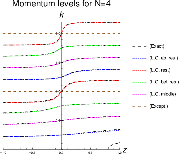
9.1 Resonant levels
By setting
| (462) |
in eq.(457), one obtains for the momentum shift:
| (463) |
Therefore, for
| (464) |
the expansion for small coupling of the total momentum reads:
| (465) |
In the above equation we have taken into account that:
| (466) |
The above choice for the indices and then gives the resonant levels:
| (467) |
Let us then define the function
| (468) |
with:
| (469) |
Note that:
| (470) |
as it should. The (still exact) equation for the momentum shift is written:
| (471) |
where we have defined the variable:
| (472) |
Note that:
| (473) |
so that reduces to in the free limit .
In terms of the complete momentum of the particle , the momentum equation above is rewritten:
| (474) |
where the function has been defined in eq.(468). The general theory of the solutions of the above equation by means of a function series or by means of a recursion equation is treated in detail in section 7, to which the reader is referred.
For concreteness sake, let us give the explicit expressions of the three recursive solutions of lowest order for the particle momentum:
| (475) | |||||
The evaluation of higher-order recursions is straightforward and is discussed, in a general form, in section 7.1. As in all previous cases, one can also use the resummation scheme for the particle momenta, which is based on a function series expansion. In addition to a direct calculation, the required functions can also be evaluated by expanding the recursive solutions in powers of the coupling , as described in 7.2.
Let us now discuss a problem occurring in the numerical evaluation of the function , which is needed for example for making a plot like fig. 10 (the red dotted curves). The direct numerical evaluation of the big round bracket on the r.h.s. of eq.(446) for gives, for :
| (476) |
The result in the last member of the above equation is incorrect for by an over-all sign, as seen by comparing with the last member of eq.(455). The error occurs because the program, for small , first basically computes the square of , always obtaining a positive number, and then computes the arithmetic (i.e. positive) square root, always obtaining again a positive number, even for . To solve this problem, one can rewrite the round bracket, for example, in the following form:
| (477) |
9.2 Non-resonant levels above the resonant ones
By setting
| (478) |
in eq.(457), one obtains for the momentum shift:
| (479) |
since, at lowest order
| (480) |
so that:
| (481) |
Then, by taking both signs positive in the general formula (446),
| (482) |
the expansion of the corresponding momentum levels reads:
| (483) |
where we have absorbed the constant inside the index by introducing the new, shifted index:
| (484) |
Therefore the positive choice for both indices gives the non-resonant levels right above the resonant ones:
| (485) |
The function , giving the recursions, is given by:
| (486) |
where:
| (487) |
Note that we have subtracted the constant from to obtain the function , since we have added the same quantity to for going to . With this subtraction, the function (linearly) goes to zero for , as it should.
For the non-resonant levels, the (still exact) momentum equation is conveniently written:
| (488) |
where we have defined the new ad-hoc variable:
| (489) |
For easy of reference, let us give the explicit expressions of the three lowest recursions:
| (490) | |||||
The evaluation of higher-order recursions is discussed in general in section 7.1. In the resummation scheme given by a function series, the required functions can be evaluated by expanding the recursive solutions in powers of the coupling , as described in 7.2.
9.3 Non-resonant levels below the resonant ones
By setting
| (491) |
in eq.(460), the pole term in the argument of the arctangent vanishes, so that:
| (492) |
By absorbing the constant term in the index , the total momentum can be written:
| (493) |
where we have defined the new, shifted index:
| (494) |
Therefore the above sign choices for the indices gives the non-resonant levels right below the resonant ones:
| (495) |
The function is given by:
| (496) |
where:
| (497) |
It is immediate to check that:
| (498) |
as it should, to properly generate recursions starting from the free-theory limit . For the constant added to and subtracted to , see the remark in the previous section.
For the recursions, the (still exact) momentum equation is conveniently written:
| (499) |
where:
| (500) |
According to the general theory described in section 7.1, the lowest three recursions explicitly read:
| (501) | |||||
The resummation scheme based on a function-series expansion can be implemented as described in section 7.2.
9.4 Non-resonant levels at the middle of two resonant levels
Finally, by setting
| (502) |
in eq.(460), one obtains for the momentum shift:
| (503) |
In the last equality we have taken into account that our branch of the arctangent is an odd function. By using eq.(320) for (the simpler repulsive case), one obtains:
| (504) |
In the above formula, one can incorporate the constant inside the index , by writing for the total momentum:
| (505) |
where we have defined:
| (506) |
Therefore the negative choice for both indices gives the non-resonant levels at the middle of two adjacent resonant levels:
| (507) |
The function , correctly vanishing at , is given by:
| (508) |
where:
| (509) |
To generate the recursions, the momentum equation is conveniently written:
| (510) |
where:
| (511) |
According to the general theory described in section 7.1, the lowest three recursions explicitly read:
| (512) | |||||
Higher-order recursions, as well as the functions to be computed in the function-series resummation scheme, can be evaluated as described in sections 7.1 and 7.2 respectively.
Let us now discuss a problem occurring in the numerical evaluation of the function . According to the second member in eq.(503), the argument of the arctangent function — the curly bracket — has a simple pole at , with a negative residue. In order to (numerically) evaluate the arctangent of a small argument for (thus obtaining a continuous function at ), it is convenient to transform the curly bracket to its inverse. By assuming (repulsive interaction), one obtains:
| (513) | |||||
9.5 Discussion
We think that the case can be reasonably considered a large- case, with a weak-coupling dynamics () resembling quasi-continuum resonance dynamics (). As we have shown, a pair of contiguous resonant levels, with indices and for , is separated by three contiguous non-resonant levels, with indices , and . A non-resonant level right above a resonant one, i.e. with , has most of its variation at and it is naturally associate to this resonant level. Similarly, a non-resonant level right below a resonant one, i.e. with , has most of its variation at and it is then naturally associated to such resonant level. Therefore, as far as resonant behavior is concerned, momentum levels group in triples, containing a resonant level in the middle and two adjacent non-resonant levels, as it occurs in the case . The non-resonant levels at the middle of two resonant levels, i.e. with , are roughly symmetrical under a sign change of the coupling, i.e. for . They do not exhibit a resonant behavior in any coupling region and therefore cannot be naturally associated to any resonant level. We may say that the levels, which are the main novelty of the case, have the role of ”separators” of contiguous resonance triplets. They are qualitatively similar to the non-resonant levels of the model.
If we consider an initial box eigenfunction contained in the small resonating cavity, analog to that in eq.(288), we expect the no-escape probability, for example, to exhibit an exponential decay in some ”intermediate” time region, as it occurs in the continuous limit .
10 Conclusions
The aim of this work was understanding how resonance dynamics emerges in finite-volume Winter (or -shell) model, from a simple oscillating behavior at (both resonant cavities having the same length), by progressively increasing the ratio of the length of the large cavity over the small one. By increasing this ratio from up to , we found new resonance phenomena emerging at each step.
Winter model in the symmetric case, , describes a system of two identical resonant cavities, weakly-coupled to each other. Therefore, in this smallest possible case, the large cavity actually has the same length as the small one. The main property of the model is that it has no non-resonant levels, but only resonant and exceptional levels.
According to a simple statistical-mechanics reasoning, the exponential decay of a resonant state with time can be considered some kind of thermalization process of this ”hot” single state immersed in a ”cold” background (or reservoir), which is composed of the huge number of the available decay final states. At infinite volume, , where the exponential decay of resonances occurs in a rather clean form and in a long time interval, the final decay states form indeed a continuum (in energy space). At large volumes, , where the available decay final states form a quasi-continuum, exponential decay of resonances is also expected to occur in a sizable time region. On the contrary, at , the level density of the large cavity is small, as it is equal to the level density of the small one, so that very few decay final states are available to an initial box eigenfunction contained in the small cavity. As a consequence, if the above statistical picture of resonance decay is correct, an initial box eigenfunction is expected to produce an oscillating behavior of the inside amplitude with time, rather than an exponential decay. The amplitude simply oscillates with time, from one cavity to the other one, back and forth.
Winter model in the double case, , in which the large cavity is two times larger than the small one, is the smallest- case expected to show some mild resonance behavior. At , the level density of the large cavity (in momentum space) is indeed two times larger than that of the small one, so that, according to the statistical picture above, the number of available final states to resonance decay is two times bigger with respect to the previous case. By going from to , the main novelty is the appearance of non-resonant levels in the spectrum of the model. Resonant and non-resonant levels, as functions of the coupling , alternate, so that they separate each other (they never cross). Since the non-resonant levels are rather symmetrical under a sign change of the coupling, namely , their growth with in the positive-coupling region is similar to that in the negative-coupling one . In general, non-resonant levels do not exhibit a resonance behavior in any coupling region. Therefore, as far as resonance dynamics is concerned, it is not possible to associate, in a natural way, a non-resonant level to a resonant one. We may say that, at , non-resonant levels have the role of ”separators” of contiguous resonance levels.
The main novelty of Winter model in the triple case, , with respect to the case, is the ”differentiation” of non-resonant levels. At , there are two non-resonant levels for each resonant level, with sub-index . The non-resonant level right above a resonant one, i.e. with , exhibits a mild resonant behavior (a roughly linear growth with the coupling ) mostly in the positive coupling region . It is therefore natural to associate such non-resonant level to the resonant level right below it. As we know from general resonance theory in the quasi-continuum , a resonant behavior, exhibited by a resonant level for small couplings is, going to larger couplings, softened and transferred to the contiguous higher non-resonant level. In a similar way, non-resonant levels right below a resonant one, i.e. with , present a mild resonant behavior for negative couplings and are naturally associated to such resonant level. Therefore a resonance of standard Winter model corresponds, in the model, to a triplet of momentum eigenstates, namely a resonant state and the two adjacent non-resonant levels. We expect an initial box eigenfunction, contained in the small cavity, to exhibit an appreciable resonant behavior, i.e. an approximate exponential decay in some limited time interval. In general, we conjecture that the ”transition” from an oscillating behavior to a resonant one is already occurred, to some extent, by going from to .
Finite-volume Winter model in the quadruple case, , presents some new qualitative features with respect to the previous, case. In the case, two contiguous resonant levels are separated by three non-resonant levels, with . The two non-resonant levels adjacent to a resonant one, having , present a similar resonant behavior to the corresponding levels of the case. Let us remark that the resonant behavior of the levels is more marked a fortiori in the model than in the one. The non-resonant levels at the middle of two resonant levels, i.e. with , are the main novelty of the transition. These levels are quite symmetrical under a change of sign of the coupling, do not exhibit a resonant behavior in any coupling region and are qualitatively similar to the non-resonant levels of the model. The main role of the levels is that of separating different triplets of levels, having a related resonance behavior, i.e. a triplet of levels with from triples of levels with We expect an initial box eigenfunction contained in the small cavity to exhibit an exponential decay in some intermediate time interval, i.e. after short-time transients (the so-called Zeno effect) and before power effects or Poincare’ recurrence take over.
To analytically understand the dynamics of the above models, we have constructed a high-energy expansion for the momenta of the particle as functions of the coupling , namely . This expansion realizes an approximate resummation of the perturbative series of the momenta, to all orders in the coupling . The high-energy expansion works much better than reasonably expected a priori, as it also works for low-energy states. Furthermore, it converges quickly with the order of the approximation and uniformly in the coupling . The fact that our expansion also converges for intermediate and large couplings is really a second, unexpected ”bonus”, because it is initially derived by assuming to be in the small-coupling domain . Technically, the good behavior of our expansion at large couplings may be due to the appearance of arctangent functions containing the coupling inside their argument.
To go in some details, we have constructed two different resummation schemes. The first scheme is based on a function-series expansion (necessarily truncated at some finite order) and has a very clear physical picture. The second scheme is based on a recursion equation, which is necessarily solved in an approximate way, by computing a finite number of recursions from the initial condition. At the first, leading order, the two resummation schemes give identical results, while they slightly differ from next-to-leading order on. Beyond leading order, it turns out that the recursive scheme realizes an approximate resummation, to all orders, of the function series generated within the first scheme. With a suggestive language, we may say that the recursive scheme ”resums the resummation” defining the function-series scheme. Because of that, we believe that the recursive scheme generally offers a more accurate approximation to the particle momenta than the function-series scheme.
Let us finally discuss some possible developments of our work which, quite generally, can be continued along different lines of investigation. Finite-volume Winter model at is the largest- case which we have analyzed with our expansion and which can be treated by means of elementary functions. By means of special functions, our high-energy expansion for the particle momenta, can be extended to analytically investigate finite-volume Winter models with . Technically the analysis is expected to be considerably more complicated than the ones in this work but is, in principle, feasible.
A similar analysis to the one presented in this work could also be made for the model considered in ref.[13], where two harmonic oscillators are coupled to each other by cutting the tails of their potentials and gluing them together. One could study, in particular, whether resonant states are described by clusters of energy levels centered around specific levels, as it happens in finite-volume Winter model. If finite-volume resonance dynamics turned out to be the same, one would get some hints about its universality. In the oscillator case, the unperturbed spectrum (free oscillators) is evenly spaced in energy space, rather than in momentum space.
A different development line involves the explicit investigation of various, intriguing time-dependent phenomena occurring in finite-volume Winter model. By considering, for example, initial box eigenfunctions localized in the small cavity, one can study the depletion and the filling of this cavity with time. Typical phenomena of resonances in a box, such as the Poincare’ recurrence or the limited decay, can be analyzed. For the same initial wavefunction, one can study the temporal evolution for different values of the coupling and of the cavities length ratio .
References
- [1] G. Gamow, ”Zur Quantentheorie der Atomkernes”, Z. Phys. 51, p. 204 (1928).
- [2] For a clear introduction to resonances, see for example: K. Gottfried, ”Quantum Mechanics”, W. A. Benjamin (1966).
- [3] L. Fonda, G. C. Ghirardi and A. Rimini, ”Decay Theory of Unstable Quantum Systems”, Rept. Prog. Phys. 41 (1978) 587, doi:10.1088/0034-4885/41/4/003.
- [4] ”Unstable states in the continuous spectra”, in Advances in Quantum Chemistry, vol.60 (2010), North Holland, edited by C. Nikolaides.
- [5] “Unstable States in the Continuous Spectra, Part II: Interpretations, Theory and Applications”, in Advances in Quantum Chemistry, vol.63 (2012), Elsevier, volume edited by C. A. Nicolaides and E. Brändas (Series Editors J. S. Sabin and E. Brändas ).
- [6] Resonances are also treated in the classic references on the matrix: R. Newton, ”Scattering of Waves and Particles”, Dover Publications, Inc. Mineola, New-York (2004); M. Goldberger and K. Watson, ”Collision Theory”, Dover Publications, Inc. Mineola, New-York (2002).
- [7] For an ”experimential” definition of resonances in quantum field theory see: L. Maiani and M. Testa, ”Unstable Systems in Relativistic Quantum Field Theory”, Ann. of Phys. vol. 263, n. 2, pag. 353 (1998); F. Giacosa, ”Non-exponential decay in quantum field theory and in quantum mechanics: the case of two (or more) decay channels”, Found. Phys. 42 (2012) 1262, arXiv:1110.5923 [nucl-th].
- [8] R. de la Madrid, ”The decay widths, the decay constants, and the branching fractions of a resonant state”, Nucl. Phys. A 940 (2015) 297, arXiv:1505.07139 [quant-ph].
- [9] L. A. Khalfin, ”Contribution to the decay theory of a quasi-stationary state”, Soviet Phys. — JETP 6, 1053 (1958); Soviet Phys. Doklady 5, 515 (1960).
- [10] E. Torrontegui et al., ”Quantum Decay at Long Times”, contribution in [4].
- [11] U. Fano, ”Effects of Configuration Interaction on Intensities and Phase Shifts”, Phys. Rev. 124, 6, p.1866 (1961).
- [12] P. W. Milonni, J. R. Ackerhalt and H. W. Galbraith, ”Exponential decay, recurrences, and quantum-mechanical spreading in a quasi-continuum model”, Phys. Rev. A 28,1 p. 32 (1983);
- [13] M. Nieto, V. Gutschihk, C. Bender, F. Cooper and D. Strottman, ”Quantum mechanical tunneling from the false vacuum: it is not as simple as you think”, LA-UR-85-1250 Preprint;
- [14] B. Gaveau and L. S. Shulman, ”Limited Quantum Decay”, J. Phys. A: Math. Gen. 28, 7359-7374 (1995);
- [15] U. G. Aglietti, ”Winter model in the quasi-continuum limit”, Int. J. Mod. Phys. A vol.35 (n.6), 2050026 (2020) (arXiv:1903.05051 [quant-ph]).
- [16] See for example: T. D. Lee, ”Particle Physics and Introduction to Field Theory”, Harwood Academic Publishers, Third Printing, Revised and Updated First Edition (1988).
- [17] S. Flugge, ”Practical Quantum Mechanics”, Springer-Verlag, Berlin (1994), problem n. 27, ”Virtual levels”.
- [18] R. G. Winter, “Evolution of a Quasi-Stationary State”, Phys. Rev. 123, n. 4, pag. 1503 (1961).
- [19] D. A. Dicus, W. W. Repko, R. F. Schwitters and T. M. Tinsley, ”Time Development of a Quasi-Stationary State”, Phys. Rev. A 65, 032116 (2002).
- [20] U. G. Aglietti and P. M. Santini, “Analysis of a Quantum Mechanical Model for Unstable Particles”, arXiv:1010.5926v2 [quant-ph] and references therein.
- [21] U. G. Aglietti and P. M. Santini, “Renormalization in the Winter Model”, Phys. Rev. A 89, 022111 (2014).
- [22] U. G. Aglietti and P. M. Santini, ”Geometry of Winter Model”, J. Math. Phys. 56 (2015) no. 6, 062104, arXiv:1503.02532 [hep-th].
- [23] R. de la Madrid, ”Numerical calculation of the decay widths, the decay constants, and the decay energy spectra of the resonances of the delta-shell potential”, Nucl. Phys. A 962 (2017) 24, arXiv:1704.00047 [quant-ph], and references therein for application of Winter model.
- [24] For an application of standard Winter model to Nuclear Physics (-decay of nuclei), see for example: E. Segre, ”Nuclei and Particles: An Introduction to Nuclear and Subnuclear Physics”, Benjamin-Cummings Pub. Co., second edition (1978).
- [25] Problem n. 19, ”Opaque division wall” in the book by S. Flugge cited in [17].
- [26] U. G. Aglietti, ”1/-expansion of resonant states”, Mod. Phys. Lett. A 31 (2016) no.25, 1650154, arXiv:1603.02857 [quant-ph].
- [27] See for example: A. H. Nayfeh and D. T. Mook, ”Non-linear Oscillations”, WILEY-VCH Verlag GmbH & Co. KGaA, Weinheim (2004).
- [28] One may consult a standard algebra textbook, such as, for example: G. M. Piacentini-Cattaneo Algebra, un approccio algoritmico, Decibel editrice, Padova (1996) (in Italian).
Appendix A Reduction of the tangent of a multiple angle
In this appendix we derive a general formula for the reduction of the tangent of a multiple angle — namely the reduction of to a rational function of of degree , where is any positive integer. This formula is used in the main body of the article for the crucial simplification of the momentum spectrum equation of the particle in all the cases.
According to De-Moivre formula:
| (514) | |||||
By equating the first and the last member of the above chain of equality’s and taking the real part on both sides of the resulting equation, one immediately obtains:
| (515) |
In a similar way, by equating the imaginary parts:
| (516) |
By dividing at each member the last equation by the previous one, one obtains:
| (517) |
Since is integer by assumption, we can apply the binomial formula to the expression in curly brackets above:
| (518) | |||||
where, to simplify the notation, we have defined
| (519) |
Since:
| (520) |
the terms with even index above are real, with alternating sign, while the odd-index terms are purely imaginary, again with alternating sign. We may therefore write:
| (521) | |||||
where by we denote the integer part of , i.e. the largest integer that is smaller than, or equal to, . By replacing the above expansions on the r.h.s. of eq.(517), the final reduction formula for the tangent of a multiple angle is obtained:
| (522) |
where:
| (523) |
The polynomial at the numerator is given by:
| (524) |
while the polynomial at the denominator reads:
| (525) |
For even , the polynomial at the numerator of the rational function, , has degree , while the polynomial at the denominator, , has degree . For odd , degrees are interchanged: has degree , while has degree . Therefore, for any , the rational function has degree .
By specifying eq.(522) to the cases , we immediately obtain:
| (526) | |||||
Appendix B General third-order algebraic equation
In this appendix we present a derivation of the formula for the zeroes of a general third-order algebraic equation. This formula involves nested square and cubic roots and rational operations and has been used to determine the momentum spectrum of Winter model in the case . As we are going to show, the solution involves a second-order auxiliary equation.
Let us then consider a general, monic third-order algebraic equation:
| (527) |
where are arbitrary complex numbers. If , the term proportional to , next to the highest power, can always be sent to zero by means of the shift
| (528) |
bringing the equation to the form (called reduced form):
| (529) |
where:
| (530) |
Next one uses the identity (cube of the binomial):
| (531) |
where and are two arbitrary complex numbers. By setting:
| (532) |
the above identity is re-written:
| (533) |
where we have defined:
| (534) |
The two equations above are easily solved for and . For example, one takes the third power of the first equation,
| (535) |
and solves it with respect to :
| (536) |
By substituting the above solution in the second equation of the system, namely , one obtains the equation
| (537) |
which is basically the bi-cubic equation
| (538) |
where we have defined:
| (539) |
Eq.(538) is an auxiliary second-order algebraic equation in , which is easily solved to give:
| (540) |
The solution for the original variable is simply obtained by taking a cubic root on both sides of the above equation:
| (541) |
Since , the quantity has the opposite sign determination of the square root with respect to :
| (542) |
The solution of the reduced equation (529) therefore reads:
| (543) |
By introducing the primitive cubic root of unity,
| (544) |
, all the three solutions of the reduced equation can be explicitly written as:
| (545) |
The solution of the original equation (527) is simply obtained by subtracting to :
| (546) |
where , and the coefficients and are given in terms of the original coefficients in eqs.(B).
Appendix C General fourth-order algebraic equation
In this appendix we sketch the derivation of the formula for the zeroes of a general fourth-order algebraic equation. Similarly to the third-order case treated in the previous appendix, this formula involves nested square and cubic roots and rational operations. It is however much more complicated than the third-order one, because it involves an auxiliary equation of third-order (rather than of second order). The general solution of the fourth-order equation has been used to determine the momentum spectrum of Winter model in the case .
A general monic fourth-order algebraic equation reads:
| (547) |
where are given complex numbers. If , by means of the shift
| (548) |
one obtains the reduced fourth-order equation:
| (549) |
where:
| (550) | |||||
The general idea is to rewrite the reduced equation in such a way that both its left-hand-side and its right-hand-side become squares of polynomials of lower degree. Let us begin with the two higher powers of , which we keep on the l.h.s.:
| (551) |
By adding to both sides of the above equation, the latter is written:
| (552) |
So, we succeeded in writing the l.h.s. as the square of a quadratic (i.e. second-degree) polynomial in (without the linear term). Now we want to write the r.h.s. as the square of a linear (i.e. first degree) polynomial in . It is clear that we have to add a term quadratic in to both sides of the above equation; in doing that, we must not spoil the perfect square on the l.h.s.. Let us add therefore to both sides of eq.(552) the quantity
| (553) |
with a still undetermined quantity, to obtain:
| (554) |
According to the above idea, we now simply choose in such a way that the r.h.s. is the square of a linear polynomial:
| (555) | |||||
By equating the first member in the above chain of equalities with the last one, one obtains the following auxiliary (general) third-order equation in :
| (556) |
with the coefficients given by:
| (557) |
The above equation can be solved by means of the general method described in the previous appendix B. Let us call
| (558) |
anyone of its solutions (note that we are free to choose any solution we like, as any solution would work). The fourth-order equation is then written:
| (559) |
By taking the square root on both sides, one obtains two second-order equations in :
| (560) |
The solutions of the above equations explicitly read:
| (561) |
The sign determination in front of the big square root has been put in parenthesis to indicate that it is an independent determination with respect to the other one. In general, therefore, four different roots are obtained, as it should.
The zeroes of the original fourth-order equation (547) are given by:
| (562) |
where is a solution of the auxiliary third-order equation (556). The coefficients of this equation are given in terms of the coefficients of the reduced fourth-order equation in eqs.(C). The latter, in turn, are given in terms of the coefficients of the original fourth-order equation in eqs.(C).