Gravitational dynamics in Higgs inflation:
Preinflation and preheating with an auxiliary field
Abstract
The dynamics of both the preinflationary and the preheating epochs for a model consisting of a Higgs inflaton plus an additional auxiliary field are studied in full General Relativity. The minimally coupled auxiliary field allows for parametric-type resonances that successfully transfer energy from the inflaton condensate to particle excitations in both fields. Depending on the interaction strengths of the fields, the broad resonance periods lead to structure formation consisting of large under/over-densities, and possibly the formation of compact objects. Moreover, when confronting the same model to multi-field inhomogeneous preinflation, the onset of inflation is shown to be a robust outcome. At relatively large Higgs values, the non-minimal coupling acts as a stabilizer, protecting the dynamics of the inflaton, and significantly reducing the impact of perturbations in other fields and matter sectors. These investigations further confirm the robustness of Higgs inflation to multi-field inhomogeneous initial conditions, while putting in evidence the formation of complex structures during the reheating.
pacs
98.80.Cq, 98.70.VcI Introduction
Cosmic inflation Starobinsky 1980; Guth 1981; Sato 1981; Linde 1982 is the current paradigm of the early Universe. It postulates an early phase where the Universe underwent over a large period of accelerated expansion. Such a period provides an explanation for today’s large scale homogeneity and flatness of the Universe. During inflation, quantum fluctuations became red-shifted, exiting the Hubble horizon at the time, and leading to a scale-invariant power spectrum of cosmological perturbations which can be matched to current observations Akrami et al. 2020; Ade et al. 2016. At later times, they provide the seeds needed for structure formation.
In a universe governed by the Einstein’s field equations, the accelerated expansion of the universe is obtained when the effective equation of state is strictly smaller than . In the slow-roll inflationary paradigm, this is typically achieved by postulating a universe dominated by a scalar field (slowly) rolling down its potential. Assuming homogeneity and isotropy, from the shape of the potential, the slow-roll conditions can be derived. When these conditions are satisfied, the energy budget is dominated by the potential energy (i.e it keeps an ), and a sustained period of slow-roll inflation occurs. Surely, assuming homogeneity and isotropy for the initial conditions of the universe is one of the main problem inflation is supposed to solve, so the initial conditions required for inflation have often been a topic of controversy, e.g. in Refs. Goldwirth and Piran 1990; Goldwirth 1991; Laguna et al. 1991; Kurki-Suonio et al. 1993; Deruelle and Goldwirth 1995 and more recently in Refs. Martin et al. 2014a; Ijjas et al. 2013; Guth et al. 2014; Easther et al. 2014; Ijjas and Steinhardt 2016; Chowdhury et al. 2019. Thus, the remaining question is; Can generic (inhomogeneous) preinflationary scenarios successfully lead to enough cosmic inflation ( efolds)?
The issue of initial conditions for inflation has been studied extensively using analytical, semi-analytical and numerical approaches (for a review see Ref. Brandenberger 2017). Full numerical relativity simulations have also been used to explore the dynamics of the preinflationary era beyond the perturbative regime. These have consisted of scenarios with a highly inhomogeneous scalar field East et al. 2016; Clough 2017 and large tensor perturbations Clough et al. 2018. The effects of concave and convex potential shapes were also studied in Ref. Aurrekoetxea et al. 2020.
In our previous paper Joana and Clesse 2021, the case of (single field) Higgs/Starobinsky preinflation was considered, containing large field gradients and inhomogeneous kinetic energies across Hubble scales. We have shown that for this model, gravitational shear and tensor modes can potentially delay the onset of inflation, but never prevent it. The question of the implications of adding extra fields is, however, still open.
The (p)reheating epoch is a necessary phase occurring after the end of inflation. It starts once the slow-roll conditions are violated and the inflaton condensate begins to oscillate around the minimum of its potential. These oscillations transfer energy to the matter sector, through parametric resonances, originating in the hot big bang plasma Traschen and Brandenberger 1990; Dolgov and Kirilova 1990. Usually, in the literature, the phase when particles are produced is known as “preheating”, while the term “reheating” is left for when the inflaton has effectively decayed and the thermalization phase begins. The reheating process has direct implications on the Cosmic Microwave Background (CMB), and current measurements are sensitive to it Martin and Ringeval 2010; Martin et al. 2015; Martin et al. 2016. For a more elaborate review on the topic, see Refs. Allahverdi et al. 2010; Tenkanen and Tomberg 2020.
The dynamics of the initial stages of preheating have been extensively studied throughout the last decade. Perturbative approaches Traschen and Brandenberger 1990; Dolgov and Kirilova 1990; Kofman et al. 1994; Kofman et al. 1997; Tsujikawa et al. 1999a; Tsujikawa et al. 1999b and numerical lattice simulations Prokopec and Roos 1997; Felder and Kofman 2001; García-Bellido et al. 2003; Amin et al. 2010; Frolov 2010; Lozanov and Amin 2014; Repond and Rubio 2016; Lozanov and Amin 2019 have been used extensively while assuming linearized Einstein gravity. Reheating involving non-minimally coupled scalar fields has also been of large interest Tsujikawa et al. 1999a; Tsujikawa et al. 1999b; van de Bruck et al. 2017; DeCross et al. 2018a; DeCross et al. 2018b; DeCross et al. 2018c; Sfakianakis and van de Vis 2019; Nguyen et al. 2019; Rubio and Tomberg 2019; van de Vis et al. 2020; Ema et al. 2017; Ema et al. 2021, and includes studies of Higgs inflation Repond and Rubio 2016; Sfakianakis and van de Vis 2019; Rubio and Tomberg 2019; Hamada et al. 2021. While lattice simulations have been capable to preserve the non-perturbative dynamics associated with inhomogeneous scalar fields, they do not consider the fully non-linear gravitational counterparts Bassett et al. 1999, whose effects on the structure formation might lead to the early formation of black holes Jedamzik et al. 2010a; Jedamzik et al. 2010b; Zhou et al. 2020. In 2019, Giblin and Tishue, in Ref. Giblin and Tishue 2019 presented the first preheating simulations in full general relativity for the canonical inflationary model. While their results disfavor the formation of compact structures, for that particular model, it shows the potential of numerical relativity to clarify the role of gravitational backreactions in the early Universe, complementary to the standard cosmological perturbation theory. In 2020, Kou et. al. in Ref. Kou et al. 2021a (see also Kou et al. 2021b) presented numerical relativity simulations for an alternative inflationary model which allowed the formation of oscillons during the preheating potentially collapsing into black holes.
In this paper, I present a set of full general relativity simulations concerning both the preinflationary and preheating epochs. The non-minimally coupled Higgs inflation model has been considered in the presence of an auxiliary scalar field. With the help of these simulations, we first ask ourselves how a full general relativistic treatment affects the resonant dynamics of preheating, and how the coupling strength of the fields affect the formation of structures during the broad resonance phase. Then, we check whether similar dynamics can be present during the preinflationary phase and, importantly, if these can undermine the beginning of inflation in the first place. It is shown that, in the presence of additional fields, the non-minimal coupling to gravity of the Higgs field allows for an efficient preheating process; a large amount of particles are produced and the formation of complex structures occurs. However, during preinflation, at large enough Higgs field values, the non-minimal coupling always acts as a stabilizer that protects the dynamics of the inflaton from inhomogeneities in other fields, ensuring the success of starting cosmic inflation.
The organization of the manuscript is as follows: in Section II the generalized covariant formalism is introduced while in Section III focus on the Higgs model. Section IV explains the numerical strategy of the simulations. The results for preheating and preinflation are presented in Sections V and VI, respectively. Additional information on the notation, code performance, initial data sets and supplementary figures are available in the appendixes.
II Covariant formalism
In this section, we consider a universe containing an arbitrary number of scalar fields , labeled by Latin capital letters . We consider a metric tensor in dimensions where Greek letters are used to label spacetime indices , using the “mostly plus metric” sign convention . The variables with an upper-bar or “hat” are being described in the Jordan frame. In these kind of models, the action in the Jordan frame is given by
| (1) |
where is the reduced Planck mass, is the determinant of the metric, is the Ricci scalar, is the scalar field potential, and contains the fields non-minimal coupling gravity , so that
| (2) |
The dynamical analysis of such systems is easier to deal with in the Einstein frame. This is done by rescaling the metric tensor, under the Weyl transformation
| (3) |
Thus, now in the Einstein frame, the action reads
| (4) |
Where is a field-space metric containing the mixing with the non-minimal coupling,
| (5) |
and the field potential has been redefined as
| (6) |
Varying the action of Eq. (4) with respect to , one can find the stress tensor and the field’s equations of motion:
| (7) |
| (8) |
where is the Alembertian operator, and are the Christoffel symbols constructed from the field-space metric .
The canonical Einstein fields denoted by are defined by solving the following system of equations
| (9) |
This transformation further simplifies the action in Eq. (4). However, finding the solution to such a system of equations is not always straightforward 11 1 In fact, finding a global transformation that solves Eqs. 9 is not possible when the field-space manifold is curved DeCross et al. 2018a. However, it is often possible to find an approximate local solution that maps both field spaces in a specific region of the field space (see section III.3)..
Thereafter, in the Einstein frame, the field equations of motion are reduced to the classical Klein-Gordon equations of the form
| (10) |
III Higgs Inflation
In this work we consider the model of (non-minimally coupled) Higgs inflation which is one of the most favored slow-roll inflation models by the latest CMB data from Planck Martin et al. 2014a. We consider a dynamical system consisting of two scalar fields and gravity. Interaction between the Higgs field and other Standard Model particles, particularly in the electroweak sector, have been ignored. The evolution has been treated classically, therefore radiative loop corrections have also been neglected. Section III.1, briefly reviews the formalism for the single-field paradigm, assuming the unitary gauge, while the implications of adding extra scalar fields are discussed in Sec. III.2.
III.1 The single-field case
The Higgs inflation model Bezrukov and Shaposhnikov 2008 postulates that the inflaton is the Higgs field from the Standard Model of particle physics, with a non-minimal coupling to gravity. The Standard Model Lagrangian, therefore, includes an extra term , where is the Ricci scalar, and is the Higgs field in the unitary gauge García-Bellido et al. 2009,
| (11) |
and is the only free parameter of the model. This term is somehow expected as it is naturally generated by quantum corrections in curved spacetime Callan et al. 1970.
In the Einstein frame, the Higgs potential reads
| (12) |
the shape of which is illustrated in Fig. 1. For the single field case, using Eq. (9), one can convert from the Jordan frame field to the canonical inflaton in the Einstein frame by solving
| (13) |
which leads to the known expression Martin et al. 2014b
| (14) |
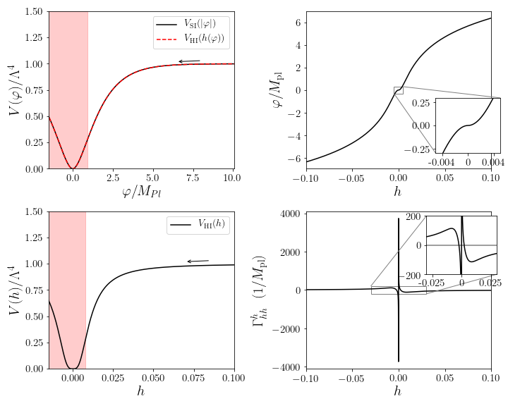
Expanding the above expression and substituting it in the potential (12), one gets, in terms of the -field,
| (15) |
where
| (16) |
is the overall amplitude of the potential.
The energy scale of inflation is given by the amplitude of the potential, . Assuming that the observable modes exited the Hubble radius at efolds before the end of inflation, the scalar and tensor perturbations of the CMB power-spectrum lead to Martin et al. 2014a. Thus, the ratio between the Higgs self-coupling and the non-minimal coupling must obey
| (17) |
Ignoring the running the Higgs self-coupling Degrassi et al. 2012, this is set to the measured value by collider physics,
Tanabashi et al. 2018.
In such a case, Eq. (17) fixes the value of the Higgs non-minimal coupling to .
At leading order, the firsts two slow-roll parameters read
| (18) | ||||
| (19) |
and as long (homogeneous) inflation is granted. In other words, the inflationary trajectory ends when , corresponding to an equation of state . Assuming that inflation lasted, at least, the minimum amount to explain the CMB observations, efolds, this implies that it should have started at a field value of (). Once cosmic inflation takes place, the field slowly rolls down the potential until the kinetic energy breaks the slow-roll conditions. The end of inflation occurs approximately at () Martin et al. 2014b, signifying the beginning of the reheating epoch.
III.2 Higgs with an auxiliary field
Let us consider now the addition of an auxiliary field , into the Higgs inflation model. To keep within the spirit of the original single-field model, in this paper, we restrict ourselves to the case where the auxiliary field is minimally coupled to gravity (). On the other hand, an interaction term is added in the action of Eq. (4),
| (20) |
where is the field-field coupling constant. This term is necessary for a parametric-type preheating to occur at the end of inflation. After this modification, the potential in Eq. (15) becomes
| (21) |
It is relevant to note that the effect of the non-minimal coupling on the potential is crucial. While in the Jordan frame the potential becomes larger at large Higgs-values , in the Einstein frame the potential tends to the constant plateau , effectively suppressing the interaction term and stabilizing the dynamics. This effect applies as well to any other possible coupling between the inflaton and other matter sources, including high energy new physics Branchina et al. 2019, which remarkably generalizes the dynamics at large field values, and thus, during preinflation Linde 1984; Linde 2018.
In this extension of the model, the canonically normalized fields in the Einstein frame are denoted by . Where represents the inflaton, and the auxiliary field.
III.3 Conversion between the fields in the Jordan and Einstein frame notation
The fact that the -field is assumed to be minimally coupled, facilitates the analysis as it simplifies the mixing between the fields and gravity. Indeed, under this assumption, the field-space metric becomes diagonal, . This is convenient because allows us to easily infer the momentum of the Einstein framed fields () the Jordan ones (), by (no index-summation implied)
| (22) |
IV Numerical strategy
The end goal of this paper is to test if Higgs inflation in the presence of an auxiliary field can begin from inhomogeneous initial conditions, and samewise if it is able to preheat the universe after the end of inflation via parametric preheating. To that end, I will be using the GRChombo numerical relativity code Clough et al. 2015; Andrade et al. 2021 to simulate the pre- and post-inflationary dynamics in full general relativity.
In the 3+1 decomposition of General Relativity Gourgoulhon 2007 the line element is written as
| (25) |
where it has been used the conformal decomposition of the metric, . The lapse and shift gauge parameters are given by and , respectively. In this section, is the metric conformal factor which relates to the cosmological scale factor as . The extrinsic curvature is also split into its conformal traceless part and the trace ,
| (26) |
It relates with the Hubble rate , in the homogeneous case, as
| (27) |
The energy-momentum tensor can be decomposed into the scalar fields’ energy density , momentum density and anisotropic tensor ,
| (28) | |||||
| (29) | |||||
| (30) | |||||
| (31) |
where is the unit normal vector to the three-dimensional slices. In analogy to the perfect fluid case with pressure , the effective equation of state can be defined by
| (32) |
In the gravity sector, the energy associated with gravitational vector and tensor modes is given by
| (33) |
and the curvature contribution to the energy budged is written in terms of the Ricci scalar (of the 3-dim metric)
| (34) |
Then one can write the Hamiltonian and momentum constraint equations as
| (35) | ||||
| (36) |
From the Arnowitt-Deser-Misner formalism, it can also be shown that the conditions to have an accelerated expansion of the universe are given when
| (37) |
Averaging overall space, we can use these conditions to determine the beginning of inflation after the preinflationary era, as well as to set the time of which preheating starts.
In the following analyses, the mean value of variable at a given time is denoted with brackets. For instance, for a given variable
| (38) |
where is the spatial volume. Similarly, the root-mean-square (rms) and the standard deviations (std) are computed like
| (39) |
These identities are used to assess the level of inhomogeneity in variable , as well as the scope of local overdensities. Some example includes the density contrast and curvature contrast which are given by
| (40) |
The scalar curvature , as well as the mean number of efolds are computed with
| (41) |
with . Here, denotes the metric conformal factor in Eq. (25).
Evolution in and Evolution in and

IV.1 Computational details
All simulations are done in a grid composed by to cells with an initial grid-size which is of the order of the Hubble size. The topology is of a 3-dimensional torus with periodic boundary conditions in all dimensions. The initial configurations assume conformal flatness, (e.g. and ),
where inhomogeneities are contained in the form of scalar field gradients, which are then compensated by the conformal factor (i.e. gravitational scalar curvature). The valid sets of initial data have been computed by solving the Hamiltonian constraint iteratively, as in most of the previous works Clough et al. 2015; Aurrekoetxea et al. 2020; Joana and Clesse 2021; Garfinkle and Mead 2020. The evolution of the system is computed in the Einstein frame by numerical integration of the BSSN equations Shibata and Nakamura 1995; Baumgarte and Shapiro 1998; Nakamura et al. 1987 in 3+1 dimensions, implemented in the GRChombo code. A more detailed explanation of the structure and validation of the code can be found in the appendixes and in Refs.Clough et al. 2015; Andrade et al. 2021.

Two different evolution schemes have been used for the numerical evolution of the fields. Simulations on the preheating epoch are evolved using the canonical Einstein fields . Therefore, at each timestep, the approximate conversions of Eq. (23) are used to recover the values of needed to evaluate the potential, Eq. (21), and its derivatives. This is done to solve dynamical instabilities occurring at , where the -field experience transients accelerations as a result of the presence of -term in the evolution equations Eq. (8) (see also Fig. 1). Despite that this issue can be overcome by shortening the time integration during the coherent linear phase, the code becomes very unstable during the broad resonance period, when the -field inhomogenizes. This issue is solved when the system is evolved using the Einstein-frame notation, and it allows us to continue the simulations for a longer time. As shown in Sec. V, both evolution schemes give numerically equivalent results. On the other hand, simulations on the preinflationary era are done using the (exact) formalism with the Jordan-framed and fields. This does not represent an issue, as does not continuously oscillate around zero and therefore the instability is not present.
V Dynamics of preheating
At the end of inflation, the inflaton field starts a period of coherent oscillations around the potential minimum. The large amplitude of the oscillations justifies a classical treatment of the inflaton field. The simulations start about -folds before the end of inflation, thus the field is considered to be initially homogeneous22 2 Simulations containing initial perturbations in the Higgs field has also been considered without significant changes in the resonance dynamics. See the Appendix E. in field value at the edge of the plateau, and is rolling down the potential with a background kinetic term. The initial values are set to
| (42) |
which is equivalent to
| (43) |
where and correspond to the fields’ momentum.
On the other hand, the auxiliary field is assumed to be in its vacuum state due to the redshift caused during inflation, where fluctuations of the field are of quantum origin. The initial state of the field is set by
| (44) |
where is the largest perturbation size, is a random phase, and the number of modes is set between and . The momentum of the -field (and ) is initially set to zero.
V.1 Parametric resonances
In the analysis, the evolution of the gravitational and scalar field sector are considered, i.e. . The later one is further decomposed into the inflaton and auxiliary field parts, by assuming
| (45) |
where the kinetic energy of the fields is used as a proxy to estimate their total energy contribution.
Because we can use two evolution schemes for the fields, namely using the Jordan or the Einstein frame definitions, let us first compare both schemes and ensure that we obtain equivalent results. In Fig. 2, this is done by direct comparison of the evolution of the energy densities shown in the top panels. The mean energy density is shown with the orange lines, while the standard deviation of the fields kinetic energies and , corresponding to the green and red lines, respectively. Additionally, the densities from the gravitational curvature (black lines) and shear (blue lines) are also shown. In the bottom panels, the mean and standard deviation of the fields and scalar curvature are shown. It is interesting to note several differences in the evolution of the fields: Because the shape of the potential is different in both representations of the field, this is reflected in the scaling of mean values of the fields Martin and Ringeval 2010. In particular, these simulations show that the mean of Higgs field scales like . On the other hand, the canonically normalized inflaton scales like . The latter is analogous to a quadratic potential around its minimum Martin and Ringeval 2010; Giblin and Tishue 2019. Differences are also noticeable when looking at the field excitations (standard deviations): in the evolution of perturbations in , the Riemann spikes that occur when are clearly visible, while for perturbations in they are hidden because of the mixing with , in the Einstein frame. In both cases, though, the scalar perturbation closely follow the fluctuations of the fields. On the other hand, the auxiliary fields behave very similarly in both schemes, and we can clearly relate the and fields. This is not surprising as the -field is chosen to be minimally coupled to gravity and therefore the mixing after the Weyl transformation is predominantly between and . All in all, we see that, for this particular case, the broad resonance of the fields occurs within efolds, where the excitations of the fields (in all frames) grow exponentially.


In a similar way, Fig. 3 shows simulations for different values in . During the broad resonance period, we find that curvature grows strictly following the excitations of the fields (the std values). The efficiency of resonances is conditioned by the -coupling, as the interaction term (Eq. 20) can be interpreted as the effective mass terms of the fields. For large couplings, , fluctuations of the field are largely suppressed during the last efolds of inflation, pushing the field down to zero. This overdamping, which is partly due to the classical treatment of the initial gradients, impedes the resonance periods at later times and preheating fails. Coupling strengths in the range of does allow preheating. However, while at larger coupling values the broad resonant phase earlier, the produced fluctuations saturate at lower energies resulting in lower energy transfer from the background field.
For even lower coupling values, , the particle production becomes inefficient (at least during the first 3-4 efolds post-inflation) and the energies associated with them fail to co-dominate the dynamics. The preheating of the universe is therefore presumably delayed to later times, but we cannot numerically explore this region.
In summary, within the assumptions of the model, a successful and fast preheating of the Universe occurs for a range in the field-field strength coupling of , with a peak efficiency of around . This is a surprising result because other studies on Higgs inflation Sfakianakis and van de Vis 2019 found that self-resonances from the Higgs, alone, effectively preheat the universe when considering linearized gravity. These simulations show that this is no longer the case when considering full gravity.
V.2 Structure formation
Structure formation starts when the energy fluctuations of the fields grow comparable to the background energy density. In our simulations, this occurs around efolds after the end of inflation, flagging the highly non-linear phase in both matter and gravitational sectors. As shown in Fig. 4, the structure consists of the region of space containing both under- and overdense energies. Overdense (underdense) scalar-field regions coexist with large local positive (negative) Ricci scalar fluctuations of the order of (), reaching even larger values for low-mass particles (i.e. ). The type of structure formed in these simulations resembles to what was reported in other works as oscillons (or transfers Lozanov and Amin 2019). Because during the structure formation the dominant energies are shifted to smaller scales, our simulations can not accurately run long enough to confirm the formation of black holes. However, other works have shown that instabilities on such oscillon-like objects, can lead to the formation of primordial black holes through self-collapse Kou et al. 2021a; Nazari et al. 2021; de Jong et al. 2022. This will be studied with dedicated simulations in future works.
VI Dynamics of preinflation
Super-Hubble perturbations Sub-Hubble perturbations


The preinflationary scenario is dependent on the initial conditions of the universe, and therefore, its properties are unknown. Arguably, in the classical regime, the primordial universe can be thought of as an inhomogeneous inflaton field that successfully leads to inflation when the kinetic and gradient energies fall below the field’s potential energy. The necessary conditions to trigger exponential expansion are a negative effective equation of state that , and a subdominant contribution of gravitational modes, i.e. Eq. (37). If these conditions are satisfied quickly enough, so that the mean field values are still in the flat part of the potential, then inflation starts.
The particular case of (single field) Higgs inflation model was considered in our previous paper, Ref. Joana and Clesse 2021. The model showed to be robust to large inhomogeneities at sub- and super-Hubble scales. Our simulations showed that highly dynamical field fluctuations source large gravitational (shear and tensor) modes that can eventually dominate the energy budget. The energy density associated with field fluctuations decays like radiation, , and these gravitational modes like
. In any case, both scalar-field and gravitational excitations eventually become subdominant in just a few -folds and inflation begins. In the following, these analyses are expanded by adding an auxiliary field.
The simulations on preinflation initially contain field gradients in both the inflaton and auxiliary fields, with perturbation in sub- and super-Hubble configurations. The initial mean value of the Higgs (inflaton) is always considered to be beyond , , so it is deeply located in the flat region of the potential. For the auxiliary field, cases with zero and non-zero mean values have been considered. The selection of these cases have been chosen so that the overall mean energy density is a few orders of magnitude larger than the energy scale of inflation, i.e. . Thus, all considered cases contain inhomogeneities well beyond the linear regime.
Figure 5 shows two example cases, at super-Hubble (left) and sub-Hubble (right) scales. In both cases, the preinflationary phase consists of a homogenization period driven by the (in average) positive expansion of the Universe. Similarly as shown in Ref. Joana and Clesse 2021, super-Hubble initial conditions tend to form trapped surfaces, or pre-inflationary black holes (PIBHs), after Hubble crossing. Because these black holes are always (much) smaller than the Hubble radius, instead of impeding inflation, they tend to facilitate it by trapping the overdense regions, thereby fastening the homogenization. On the other hand, at sub-Hubble scales, perturbation modes transit back-and-forth between gradients and kinetic energies, effectively making the energy density scale like radiation . In that scenario, the optimal conditions for triggering inflation look like a dynamical attractor, and cosmic inflation starts within a few efolds.
Interestingly, in the presence of the auxiliary (spectator) field, these oscillations also trigger energy transfer between the (Jordan framed-) Higgs and the auxiliary field. However, these dynamics do not originate in enhancement of structures like in preheating, because now at field values , the non-minimal coupling of the Higgs has the effect of significantly reducing the impact of the (minimally coupled) auxiliary field when seen in the Einstein frame. This effect can be observed in Fig. 5, where even when perturbations in the -field are larger than in the -field (see Fig. 5 middle panels), the dynamical term is always orders of magnitude smaller in the auxiliary field . The suppression effect comes from the mixing, which is introduced by the field-space metric lower than unity, i.e. and becomes orders of magnitude smaller for large enough -field values (e.g. for ). This suppression factor should apply to all other possible matter components that are minimally coupled to gravity.
VI.1 On the initial conditions for inflation
In this paper we have extended previous works on testing the initial conditions for inflation by including the interplay of an extra (minimally coupled) scalar field. We have tested cases when the initial configuration of the inflation is deeply inhomogeneous but with its mean-field value inside the slow-roll region of the potential. In the context of Higgs inflation, this corresponds to a mean value close to the plateau. Initial states where the mean-field is in the non-inflationary region (i.e. in the bottom of the potential) have not been considered as these cases should not lead to inflationary regions, as tested in Ref. Joana and Clesse 2021. This is because gradients terms make the fields oscillate around the mean value, thus these inhomogeneities are not capable of driving the field up to the plateau. One could still consider large field inhomogeneities which spans the scalar field into the potential’s plateau, however these perturbations are necessarily super-Hubble (at sub-Planckian gradient energies) and, thus, these regions can be treated as separate universes. This is particular to Higgs inflation, as the plateau starts at .
Our initial settings have also assumed a conformally flat expanding universe. These scenarios corresponds to the case with only scalar perturbations in the gravitational part, (i.e. without vector and tensor gravitational modes). This is related to the choice of considering a null kinetic term in the initial hypersurface, which can be seen as a rather “special” slicing choice at the instantaneous initial time where scalar-field kinetic terms have been gauged away, trivially satisfying the momentum constraint Eq. (36). Because these initial setting are highly dynamical, this kind of slicing is not stable and once the system is time-evolved both gravitational modes and scalar field kinetic terms are quickly generated, leading to a less symmetric inhomogeneous system. In particular, one could have chosen an analogous situation with initially homogeneous field values but with largely inhomogeneous kinetic terms which would raise scalar-field inhomogeneities in the immediate time evolution Joana and Clesse 2021. Because the minimally coupled fields are energetically subdominant at high enough Higgs values, the previous picture still holds beyond the single-field case.
Nonetheless, there are still several limitations with such initial settings. The assumption on conformal flatness only allow for gravitational perturbations risen by the scalar field evolution, and therefore independent large tensor metric perturbation are ignored. Studying these cases requires solving (non-trivially) both the Hamiltonian and momentum constraints and future works will deal with this challenge. In addition, this work has assumed that only the Higgs field has a non-minimal coupling to gravity, serving as a reference for other more specific models like quintessential Higgs inflation Es-haghi and Sheykhi 2020, two Higgs doublet models Lee et al. 2022, etc.
Still, systems with two or more non-minimally coupled fields can show a much richer dynamical evolution during (pre-)inflation; Exploring complex trajectories in field space and possibly including multiple inflationary phases at distinct energy stages. All these considerations are left to future works.
Under the previous considerations, in all the considered cases, we find common dynamical patterns of the Higgs pre-inflationary era. This phase can be described as a homogenization era with a varying inhomogeneous equation of state, which effectively correspond to a radiation dominated universe . Once the scalar-field falls below the energy scale of the inflationary potential, the equation of state tends to a de-Sitter Universe with , satisfying the first condition for inflation, i.e. Eq. (37). It has also been shown that strong field dynamics near the Hubble scales develop large gravitational modes that potentially influence the expansion of the Universe until they become subdominant. These modes effectively delay the beginning of inflation, but do not prevent it. Moreover, during the pre-inflationary era, lasting efolds, the variation on the average value of the inflaton is negligible, which prevents the “overshooting” problem seen in other models Aurrekoetxea et al. 2020. All these considerations make me conclude that, under the considered settings, the Higgs inflation model is very robust to the inhomogeneous multi-field initial conditions of the pre-inflationary era.
VII Conclusions
In this paper, I have used fully general relativistic simulations to investigate the robustness of the Higgs inflation model to inhomogeneous multi-field initial conditions. Specifically, in the presence of additional field couplings, these being necessary for a parametric-type reheating.
It is shown that, at large enough Higgs values, the non-minimal coupling of the Higgs protects the dynamics of the inflaton by diminishing the impact of couplings to other fields and matter sectors. And, as shown in Ref. Joana and Clesse 2021, the dynamics from gravitational shear and tensor modes can only delay, but not prevent, cosmic inflation.
Additionally, simulations on the preheating dynamics of the two-field system were presented where full gravitational backreactions in the metric have been considered. As expected, it is shown that the efficiency of the preheating is conditioned to coupling strength between the fields. In particular, for such a simple model, it was found the preheating of the Universe within the first efolds post-inflation to occur for couplings in the range of . On the other hand, self-resonance from the Higgs alone, fails to reheat the Universe within the first efolds after inflation.
These simulations have also shown the formation of complex structures during the preheating, consisting in large under/overdensities as well as strong positive/negative (local) curvature regions, suggesting the possibility of (seeding) later formation of compact structures like primordial black holes. Nonetheless, these results should be taken cautiously as further investigations, including dedicated numerical simulations, are necessary to accurately resolve these highly non-linear objects.
Future works are also necessary to study more realistic preheating scenarios, including the Higgs couplings to the Standard Model particles. These are important, because they potentially could shorten the preheating within one fold after inflation Ema et al. 2017; Ema et al. 2021, if metric backreactions allow it. Other interesting aspects to be studied are the emission of gravitational waves - and possible amplification effectsLin and Sasaki 2016; Lozanov and Amin 2019; Zhou et al. 2020; Cai et al. 2021. Importantly, some of the described phenomena are expected to be in the observable range of future gravitational-wave experiments.
VIII Acknowledgments
The author warmly thanks Christophe Ringeval and Sebastien Clesse for helpful comments and support, as well as Pierre Auclair, Tiago França, Miren Radia, Josu Aurrekoetxea, Katy Clough and Eugene Lim for useful discussions. He is also in gratitude to all members of the GRChombo team (https://www.grchombo.org/#people) for their work and maintenance on the code. This work is supported by the FRIA Grant No.1.E.070.19F of the Belgian Fund for Research, F.R.S.-FNRS. Computational resources have been provided by the Julich Supercomputing Center JUWELS HPC under PRACE grant Tier-0 Proposal No. 202022535, the Consortium des Équipements de Calcul Intensif (CÉCI) under Grant No. 2.5020.11 by the Walloon Region. Parallel code developments were done on the CURL cosmo clusters at UCLouvain, funded by the “Fonds de la Recherche Scientifique - FNRS” under Grant No. T.0198.19. Analysis and visualizations employed the Visit Bethel et al. 2012 and yt-project Turk et al. 2010 software packages.
References
- Starobinsky (1980) A. Starobinsky, Physics Letters B 91, 99 (1980), ISSN 0370-2693, URL https://www.sciencedirect.com/science/article/pii/037026938090670X.
- Guth (1981) A. H. Guth, Phys. Rev. D 23, 347 (1981), URL https://link.aps.org/doi/10.1103/PhysRevD.23.347.
- Sato (1981) K. Sato, Monthly Notices of the Royal Astronomical Society 195, 467 (1981), ISSN 0035-8711, eprint https://academic.oup.com/mnras/article-pdf/195/3/467/4065201/mnras195-0467.pdf, URL https://doi.org/10.1093/mnras/195.3.467.
- Linde (1982) A. Linde, Physics Letters B 108, 389 (1982), ISSN 0370-2693, URL https://www.sciencedirect.com/science/article/pii/0370269382912199.
- Akrami et al. (2020) Y. Akrami, F. Arroja, M. Ashdown, J. Aumont, C. Baccigalupi, M. Ballardini, A. J. Banday, R. B. Barreiro, N. Bartolo, and et al., Astronomy & Astrophysics 641, A10 (2020), ISSN 1432-0746, URL http://dx.doi.org/10.1051/0004-6361/201833887.
- Ade et al. (2016) P. A. R. Ade, N. Aghanim, M. Arnaud, F. Arroja, M. Ashdown, J. Aumont, C. Baccigalupi, M. Ballardini, A. J. Banday, and et al., Astronomy & Astrophysics 594, A20 (2016), ISSN 1432-0746, URL http://dx.doi.org/10.1051/0004-6361/201525898.
- Goldwirth and Piran (1990) D. S. Goldwirth and T. Piran, Phys. Rev. Lett. 64, 2852 (1990).
- Goldwirth (1991) D. S. Goldwirth, Phys. Rev. D43, 3204 (1991).
- Laguna et al. (1991) P. Laguna, H. Kurki-Suonio, and R. A. Matzner, Phys. Rev. D44, 3077 (1991).
- Kurki-Suonio et al. (1993) H. Kurki-Suonio, P. Laguna, and R. A. Matzner, Phys. Rev. D48, 3611 (1993), eprint astro-ph/9306009.
- Deruelle and Goldwirth (1995) N. Deruelle and D. S. Goldwirth, Phys. Rev. D51, 1563 (1995), eprint gr-qc/9409056.
- Martin et al. (2014a) J. Martin, C. Ringeval, R. Trotta, and V. Vennin, JCAP 1403, 039 (2014a), eprint 1312.3529.
- Ijjas et al. (2013) A. Ijjas, P. J. Steinhardt, and A. Loeb, Physics Letters B 723, 261–266 (2013), ISSN 0370-2693, URL http://dx.doi.org/10.1016/j.physletb.2013.05.023.
- Guth et al. (2014) A. H. Guth, D. I. Kaiser, and Y. Nomura, Physics Letters B 733, 112–119 (2014), ISSN 0370-2693, URL http://dx.doi.org/10.1016/j.physletb.2014.03.020.
- Easther et al. (2014) R. Easther, L. C. Price, and J. Rasero, JCAP 1408, 041 (2014), eprint 1406.2869.
- Ijjas and Steinhardt (2016) A. Ijjas and P. J. Steinhardt, Classical and Quantum Gravity 33, 044001 (2016), ISSN 1361-6382, URL http://dx.doi.org/10.1088/0264-9381/33/4/044001.
- Chowdhury et al. (2019) D. Chowdhury, J. Martin, C. Ringeval, and V. Vennin, Phys. Rev. D 100, 083537 (2019), eprint 1902.03951.
- Brandenberger (2017) R. Brandenberger, International Journal of Modern Physics D 26, 1740002 (2017), ISSN 1793-6594, URL http://dx.doi.org/10.1142/S0218271817400028.
- East et al. (2016) W. E. East, M. Kleban, A. Linde, and L. Senatore, Journal of Cosmology and Astroparticle Physics 2016, 010 (2016), URL https://doi.org/10.1088%2F1475-7516%2F2016%2F09%2F010.
- Clough (2017) K. Clough, Ph.D. thesis, King’s Coll. London, Cham (2017), eprint 1704.06811.
- Clough et al. (2018) K. Clough, R. Flauger, and E. A. Lim, JCAP 2018, 065 (2018), eprint 1712.07352.
- Aurrekoetxea et al. (2020) J. C. Aurrekoetxea, K. Clough, R. Flauger, and E. A. Lim, Journal of Cosmology and Astroparticle Physics 2020, 030–030 (2020), ISSN 1475-7516, URL http://dx.doi.org/10.1088/1475-7516/2020/05/030.
- Joana and Clesse (2021) C. Joana and S. Clesse, Phys. Rev. D 103, 083501 (2021), URL https://link.aps.org/doi/10.1103/PhysRevD.103.083501.
- Traschen and Brandenberger (1990) J. H. Traschen and R. H. Brandenberger, Phys. Rev. D 42, 2491 (1990), URL https://link.aps.org/doi/10.1103/PhysRevD.42.2491.
- Dolgov and Kirilova (1990) A. D. Dolgov and D. P. Kirilova, Soviet Journal of Nuclear Physics 51, 172 (1990).
- Martin and Ringeval (2010) J. Martin and C. Ringeval, Physical Review D 82 (2010), ISSN 1550-2368, URL http://dx.doi.org/10.1103/PhysRevD.82.023511.
- Martin et al. (2015) J. Martin, C. Ringeval, and V. Vennin, Physical Review Letters 114 (2015), ISSN 1079-7114, URL http://dx.doi.org/10.1103/PhysRevLett.114.081303.
- Martin et al. (2016) J. Martin, C. Ringeval, and V. Vennin, Physical Review D 93 (2016), ISSN 2470-0029, URL http://dx.doi.org/10.1103/PhysRevD.93.103532.
- Allahverdi et al. (2010) R. Allahverdi, R. Brandenberger, F.-Y. Cyr-Racine, and A. Mazumdar, Annual Review of Nuclear and Particle Science 60, 27–51 (2010), ISSN 1545-4134, URL http://dx.doi.org/10.1146/annurev.nucl.012809.104511.
- Tenkanen and Tomberg (2020) T. Tenkanen and E. Tomberg, JCAP 04, 050 (2020), eprint 2002.02420.
- Kofman et al. (1994) L. Kofman, A. Linde, and A. A. Starobinsky, Physical Review Letters 73, 3195–3198 (1994), ISSN 0031-9007, URL http://dx.doi.org/10.1103/PhysRevLett.73.3195.
- Kofman et al. (1997) L. Kofman, A. Linde, and A. A. Starobinsky, Physical Review D 56, 3258–3295 (1997), ISSN 1089-4918, URL http://dx.doi.org/10.1103/PhysRevD.56.3258.
- Tsujikawa et al. (1999a) S. Tsujikawa, K.-i. Maeda, and T. Torii, Phys. Rev. D 60, 123505 (1999a), URL https://link.aps.org/doi/10.1103/PhysRevD.60.123505.
- Tsujikawa et al. (1999b) S. Tsujikawa, K.-i. Maeda, and T. Torii, Phys. Rev. D 60, 063515 (1999b), URL https://link.aps.org/doi/10.1103/PhysRevD.60.063515.
- Prokopec and Roos (1997) T. Prokopec and T. G. Roos, Physical Review D 55, 3768–3775 (1997), ISSN 1089-4918, URL http://dx.doi.org/10.1103/PhysRevD.55.3768.
- Felder and Kofman (2001) G. Felder and L. Kofman, Physical Review D 63 (2001), ISSN 1089-4918, URL http://dx.doi.org/10.1103/PhysRevD.63.103503.
- García-Bellido et al. (2003) J. García-Bellido, M. García Pérez, and A. González-Arroyo, Physical Review D 67 (2003), ISSN 1089-4918, URL http://dx.doi.org/10.1103/PhysRevD.67.103501.
- Amin et al. (2010) M. A. Amin, R. Easther, and H. Finkel, Journal of Cosmology and Astroparticle Physics 2010, 001–001 (2010), ISSN 1475-7516, URL http://dx.doi.org/10.1088/1475-7516/2010/12/001.
- Frolov (2010) A. V. Frolov, Classical and Quantum Gravity 27, 124006 (2010), ISSN 1361-6382, URL http://dx.doi.org/10.1088/0264-9381/27/12/124006.
- Lozanov and Amin (2014) K. D. Lozanov and M. A. Amin, Physical Review D 90 (2014), ISSN 1550-2368, URL http://dx.doi.org/10.1103/PhysRevD.90.083528.
- Repond and Rubio (2016) J. Repond and J. Rubio, Journal of Cosmology and Astroparticle Physics 2016, 043–043 (2016), ISSN 1475-7516, URL http://dx.doi.org/10.1088/1475-7516/2016/07/043.
- Lozanov and Amin (2019) K. D. Lozanov and M. A. Amin, Physical Review D 99 (2019), ISSN 2470-0029, URL http://dx.doi.org/10.1103/PhysRevD.99.123504.
- van de Bruck et al. (2017) C. van de Bruck, P. Dunsby, and L. E. Paduraru, International Journal of Modern Physics D 26, 1750152 (2017), ISSN 1793-6594, URL http://dx.doi.org/10.1142/S0218271817501528.
- DeCross et al. (2018a) M. P. DeCross, D. I. Kaiser, A. Prabhu, C. Prescod-Weinstein, and E. I. Sfakianakis, Physical Review D 97 (2018a), ISSN 2470-0029, URL http://dx.doi.org/10.1103/PhysRevD.97.023526.
- DeCross et al. (2018b) M. P. DeCross, D. I. Kaiser, A. Prabhu, C. Prescod-Weinstein, and E. I. Sfakianakis, Physical Review D 97 (2018b), ISSN 2470-0029, URL http://dx.doi.org/10.1103/PhysRevD.97.023527.
- DeCross et al. (2018c) M. P. DeCross, D. I. Kaiser, A. Prabhu, C. Prescod-Weinstein, and E. I. Sfakianakis, Physical Review D 97 (2018c), ISSN 2470-0029, URL http://dx.doi.org/10.1103/PhysRevD.97.023528.
- Sfakianakis and van de Vis (2019) E. I. Sfakianakis and J. van de Vis, Physical Review D 99 (2019), ISSN 2470-0029, URL http://dx.doi.org/10.1103/PhysRevD.99.083519.
- Nguyen et al. (2019) R. Nguyen, J. van de Vis, E. I. Sfakianakis, J. T. Giblin, and D. I. Kaiser, Physical Review Letters 123 (2019), ISSN 1079-7114, URL http://dx.doi.org/10.1103/PhysRevLett.123.171301.
- Rubio and Tomberg (2019) J. Rubio and E. S. Tomberg, Journal of Cosmology and Astroparticle Physics 2019, 021–021 (2019), ISSN 1475-7516, URL http://dx.doi.org/10.1088/1475-7516/2019/04/021.
- van de Vis et al. (2020) J. van de Vis, R. Nguyen, E. I. Sfakianakis, J. T. Giblin, and D. I. Kaiser, Physical Review D 102 (2020), ISSN 2470-0029, URL http://dx.doi.org/10.1103/PhysRevD.102.043528.
- Ema et al. (2017) Y. Ema, R. Jinno, K. Mukaida, and K. Nakayama, Journal of Cosmology and Astroparticle Physics 2017, 045–045 (2017), ISSN 1475-7516, URL http://dx.doi.org/10.1088/1475-7516/2017/02/045.
- Ema et al. (2021) Y. Ema, R. Jinno, K. Nakayama, and J. van de Vis, Physical Review D 103 (2021), ISSN 2470-0029, URL http://dx.doi.org/10.1103/PhysRevD.103.103536.
- Hamada et al. (2021) Y. Hamada, K. Kawana, and A. Scherlis, Journal of Cosmology and Astroparticle Physics 2021, 062 (2021), ISSN 1475-7516, URL http://dx.doi.org/10.1088/1475-7516/2021/03/062.
- Bassett et al. (1999) B. A. Bassett, D. I. Kaiser, and R. Maartens, Physics Letters B 455, 84–89 (1999), ISSN 0370-2693, URL http://dx.doi.org/10.1016/S0370-2693(99)00478-5.
- Jedamzik et al. (2010a) K. Jedamzik, M. Lemoine, and J. Martin, Journal of Cosmology and Astroparticle Physics 2010, 034–034 (2010a), ISSN 1475-7516, URL http://dx.doi.org/10.1088/1475-7516/2010/09/034.
- Jedamzik et al. (2010b) K. Jedamzik, M. Lemoine, and J. Martin, Journal of Cosmology and Astroparticle Physics 2010, 021–021 (2010b), ISSN 1475-7516, URL http://dx.doi.org/10.1088/1475-7516/2010/04/021.
- Zhou et al. (2020) Z. Zhou, J. Jiang, Y.-F. Cai, M. Sasaki, and S. Pi, Physical Review D 102 (2020), ISSN 2470-0029, URL http://dx.doi.org/10.1103/PhysRevD.102.103527.
- Giblin and Tishue (2019) J. T. Giblin and A. J. Tishue, Phys. Rev. D 100, 063543 (2019), URL https://link.aps.org/doi/10.1103/PhysRevD.100.063543.
- Kou et al. (2021a) X.-X. Kou, C. Tian, and S.-Y. Zhou, Class. Quant. Grav. 38, 045005 (2021a), eprint 1912.09658.
- Kou et al. (2021b) X.-X. Kou, J. B. Mertens, C. Tian, and S.-Y. Zhou (2021b), eprint 2112.07626.
- Bezrukov and Shaposhnikov (2008) F. L. Bezrukov and M. Shaposhnikov, Phys. Lett. B 659, 703 (2008), eprint 0710.3755.
- García-Bellido et al. (2009) J. García-Bellido, D. G. Figueroa, and J. Rubio, Physical Review D 79 (2009), ISSN 1550-2368, URL http://dx.doi.org/10.1103/PhysRevD.79.063531.
- Callan et al. (1970) J. Callan, Curtis G., S. Coleman, and R. Jackiw, Annals of Physics 59, 42 (1970).
- Martin et al. (2014b) J. Martin, C. Ringeval, and V. Vennin, Physics of the Dark Universe 5-6, 75 (2014b), ISSN 2212-6864, URL https://www.sciencedirect.com/science/article/pii/S2212686414000053.
- Degrassi et al. (2012) G. Degrassi, S. D. Vita, J. Elias-Miró, J. R. Espinosa, G. F. Giudice, G. Isidori, and A. Strumia, Journal of High Energy Physics 2012 (2012), URL https://doi.org/10.1007%2Fjhep08%282012%29098.
- Tanabashi et al. (2018) M. Tanabashi, K. Hagiwara, K. Hikasa, K. Nakamura, Y. Sumino, F. Takahashi, J. Tanaka, K. Agashe, G. Aielli, C. Amsler, et al. (Particle Data Group), Phys. Rev. D 98, 030001 (2018), URL https://link.aps.org/doi/10.1103/PhysRevD.98.030001.
- Branchina et al. (2019) V. Branchina, E. Bentivegna, F. Contino, and D. Zappalà, Physical Review D 99 (2019), ISSN 2470-0029, URL http://dx.doi.org/10.1103/PhysRevD.99.096029.
- Linde (1984) A. D. Linde, Lett. Nuovo Cim. 39, 401 (1984).
- Linde (2018) A. Linde, Found. Phys. 48, 1246 (2018), eprint 1710.04278.
- Clough et al. (2015) K. Clough, P. Figueras, H. Finkel, M. Kunesch, E. A. Lim, and S. Tunyasuvunakool, Classical and Quantum Gravity 32, 245011 (2015), ISSN 1361-6382, eprint 1503.03436, URL http://dx.doi.org/10.1088/0264-9381/32/24/245011.
- Andrade et al. (2021) T. Andrade, L. A. Salo, J. C. Aurrekoetxea, J. Bamber, K. Clough, R. Croft, E. de Jong, A. Drew, A. Duran, P. G. Ferreira, et al., Journal of Open Source Software 6, 3703 (2021), URL https://doi.org/10.21105/joss.03703.
- Gourgoulhon (2007) E. Gourgoulhon (2007), eprint gr-qc/0703035.
- Garfinkle and Mead (2020) D. Garfinkle and L. Mead, Physical Review D 102 (2020), ISSN 2470-0029, URL http://dx.doi.org/10.1103/PhysRevD.102.044022.
- Shibata and Nakamura (1995) M. Shibata and T. Nakamura, Phys. Rev. D 52, 5428 (1995), URL https://link.aps.org/doi/10.1103/PhysRevD.52.5428.
- Baumgarte and Shapiro (1998) T. W. Baumgarte and S. L. Shapiro, Physical Review D 59 (1998), ISSN 1089-4918, URL http://dx.doi.org/10.1103/PhysRevD.59.024007.
- Nakamura et al. (1987) T. Nakamura, K. Oohara, and Y. Kojima, Progress of Theoretical Physics Supplement 90, 1 (1987), ISSN 0375-9687, URL https://doi.org/10.1143/PTPS.90.1.
- Nazari et al. (2021) Z. Nazari, M. Cicoli, K. Clough, and F. Muia, Journal of Cosmology and Astroparticle Physics 2021, 027 (2021), ISSN 1475-7516, URL http://dx.doi.org/10.1088/1475-7516/2021/05/027.
- de Jong et al. (2022) E. de Jong, J. C. Aurrekoetxea, and E. A. Lim, Journal of Cosmology and Astroparticle Physics 2022, 029 (2022), URL https://doi.org/10.1088%2F1475-7516%2F2022%2F03%2F029.
- Es-haghi and Sheykhi (2020) M. Es-haghi and A. Sheykhi (2020), eprint 2012.08035.
- Lee et al. (2022) S. M. Lee, T. Modak, K.-y. Oda, and T. Takahashi, Eur. Phys. J. C 82, 18 (2022), eprint 2108.02383.
- Lin and Sasaki (2016) C. Lin and M. Sasaki, Physics Letters B 752, 84–88 (2016), ISSN 0370-2693, URL http://dx.doi.org/10.1016/j.physletb.2015.11.021.
- Cai et al. (2021) Y.-F. Cai, J. Jiang, M. Sasaki, V. Vardanyan, and Z. Zhou, Phys. Rev. Lett. 127, 251301 (2021), URL https://link.aps.org/doi/10.1103/PhysRevLett.127.251301.
- Bethel et al. (2012) E. W. Bethel, H. Childs, and C. Hansen, High Performance Visualization: Enabling Extreme-Scale Scientific Insight (Chapman; Hall/CRC, 2012), 1st ed., ISBN 1439875723.
- Turk et al. (2010) M. J. Turk, B. D. Smith, J. S. Oishi, S. Skory, S. W. Skillman, T. Abel, and M. L. Norman, The Astrophysical Journal Supplement Series 192, 9 (2010), ISSN 1538-4365, URL http://dx.doi.org/10.1088/0067-0049/192/1/9.
- Baker et al. (2006) J. G. Baker, J. Centrella, D.-I. Choi, M. Koppitz, and J. van Meter, Physical Review Letters 96 (2006), ISSN 1079-7114, URL http://dx.doi.org/10.1103/PhysRevLett.96.111102.
- Campanelli et al. (2006) M. Campanelli, C. O. Lousto, P. Marronetti, and Y. Zlochower, Physical Review Letters 96 (2006), ISSN 1079-7114, URL http://dx.doi.org/10.1103/PhysRevLett.96.111101.
Appendix A BSSN formalism of numerical relativity
In this work, we solve the BSSN formulation of the Einstein equations using GRChombo Clough et al. 2015; Andrade et al. 2021, a multipurpose numerical relativity code. In the context of the 3+1 decomposition of General Relativity, the line element reads
| (46) |
where is the metric of the 3-dimensional hypersurface, and the lapse and shift gauge parameters are given by and respectively. A further conformal decomposition of the 3-metric follows,
| (47) |
where and are two different parametrisations of the metric conformal factor. While the former is used during the temporal integration, the latter is preferred when constructing the initial conditions. The extrinsic curvature is thus split in and , respectively, the conformal traceless part and its trace,
| (48) |
In addition, the first spatial derivatives of the metric are considered as dynamical variables
| (49) |
where are the Christoffel symbols associated with the conformal metric .
A.1 Evolution equations
The evolution equations for the BSSN variables are then given by
| (50) | ||||
| (51) | ||||
| (52) |
| (53) | ||||
| (54) |
where the superscript denotes the trace-free parts of tensors, with being the (3-dimensional) Ricci tensor. The 3+1 decomposition of the energy-momentum tensor gives
| (55) | |||||
| (56) | |||||
| (57) | |||||
| (58) |
where is the unit normal vector to the three-dimensional slices.
The Hamiltonian and momentum constraints,
| (59) | ||||
| (60) |
where is the Ricci scalar, are only solved explicitly when constructing initial data. However, they are also monitored during the time evolution in order to ensure that there is no significant deviations from General Relativity.
A.2 Gauge choice and singularity avoidance
The gauge parameters are initially set to and and then evolved in accordance with the moving puncture gauge Baker et al. 2006; Campanelli et al. 2006, for which evolution equations are
| (61) | |||||
| (62) | |||||
| (63) |
where the constants and are conveniently chosen to improve the numerical stability. This way, and are boosted in the problematic regions with strongly growing extrinsic curvature and spatial derivatives of the three-metric . The goal of this gauge is to prevent the code from resolving the central singularity of any black hole that may eventually form, as well as to prevent coordinate singularities on converging geodesics.
A.3 Scalar field equations
For the Einstein frame canonical scalar field , the energy-momentum tensor is given by
| (64) |
The scalar field dynamics is governed by the the Klein-Gordon equation, split into two first order equations for the field and its momentum
| (65) | ||||
| (66) | ||||
| (67) |
Still in the Einstein frame, but with the Jordan defined scalar fields , the energy momentum is written as
| (68) |
and then the evolution equations are read
| (69) | ||||
| (70) | ||||
If instead, the system is evolved using the Einstein frame notation for the scalar fields , the energy tensor simplifies to
| (71) |
and then, the evolution equations are given by
| (72) | ||||
| (73) | ||||
Appendix B Field-space metric and Christoffel symbols
Given for a two-field model, with non-minimal couplings , the field-space metric in the Einstein frame, takes the form
| (74) |
| (75) |
where is defined as
| (76) |
The Christoffel symbols for this field space take the form
| (77) |
Appendix C Scalar fields in the Jordan and Einstein frame notation
Transforming from the scalar fields in the Jordan frame notation to the Einstein frame once is done by finding an approximate solution to the following system of equations
| (78) |
Assuming two Jordan scalar fields, the Higgs with non-minimal coupling and an auxiliary field with non-minimal coupling . Then we search for a transformation into the Einstein frame such as . Assuming , the above mentioned system of equation simplifies to
| (79) | ||||
| (80) | ||||
| (81) |
By assuming and implies that, in the range of validity of this approximation,
| (82) | ||||
| (83) |
While the first identity is trivially satisfied, the second one (83) is not, because the approximation proposes the solution to be . Thus, the validity of these approximation depend on the region in consideration of the field space, as shown in shown in Fig. 6. In general, the parameter space when this assumptions are valid is generally at when , and when . These regions corresponds to .

Appendix D Code validation and convergence tests
The validation of the code is done by monitoring the constraint equations. The relative Hamiltonian constraint is defined as follows
| (84) |
where
| (85) |
These quantity has been computed for all simulations, which is shown in Fig. 7. Convergence tests using different grid-size resolutions are shown in Fig. 8.
Appendix E Auxiliary figures
In this appendix, we include additional figures corresponding to alternative simulations constructed with some variation in the initial conditions. For the simulations on preheating, we tested whether the inclusion of initial perturbations in the Higgs field induce changes during the resonance period, in particular in the low limit as perturbations in the Higgs field during the last efold of inflation could have been diminished. In addition, a larger initial box size was also considered. These modifications, as shown in Fig. 9, do not significantly change the resonance dynamics of the preheating process. Similarly, alternative initial conditions for the pre-inflationary era are shown in Fig. 10, where larger box sizes where tested, as well as different patterns in the initial field gradients. These simulations also lead to the same conclusions explained in section VI.1.


