A ring of spikes

The goal of this paper is to study a solution to reaction-diffusion model consisting of a ring of spikes. This configuration is highly symmetric, which allows for an in-depth analysis of its stability properties. For simplicity, we will concentrate on the Schnakenberg model schnakenberg1979simple although similar techniques can be extended to other models. We study the following version of the Schnakenberg model xie2017moving:

$$u_{t}=\varepsilon^{2}\Delta u-u+u^{2}v,\ \ \ \ 0=\Delta v+A-u^{2}v\frac{1}{\varepsilon^{2}}\frac{1}{\log\varepsilon^{-1}}$$

(1)

with the usual Neumann boundary conditions inside a radially symmetric domain $\Omega_{b},$ which we take to be either a disk or an annulus of inner radius $b$ and outer radius 1:

$$\Omega_{b}=\left\{x:b<\left|x\right|<1\right\}.$$

(2)

An example of a ring of 6 spikes inside a unit disk is shown in Figure 1 (left).

The general problem of $N$ spikes in 2D and their stability was considered in numerous papers. See wei2008stationary for a good review and stability computations for the Schnakenberg model. See also muratov2001spike; ward2002existence; wei2003existence; chen2010; kolokolnikov2009spot; xie2017moving; wong2020spot for related results in two-dimesions. As is well known, there are two types of instabilities that are possible: due to large $(O(1)$) or small $(O(\varepsilon^{2})$) eigenvalues. Instability triggered by large eigenvalues induces a “structural” or spike profile instability on an O(1) time scale. Numerically, this instability is observed to be subcritical (see also kolokolnikov2021competition; kolokolnikov2020stable for analysis of criticality in 1D) and quickly leads to a reduction in the number of spikes. The small-eigenvalue instability induces a spike motion on a slow timescale. Its criticality depends on the number of spikes as well as domain shape.

In paper wei2008stationary, the authors analysed general equilibrium configurations of $N$ spikes in 2D. They derived a simple threshold on the feed rate $A$ such that an instability with respect to large eigenvalues is triggered as $A$ is decreased past that threshold. For for a general spike equilibrium subject to a natural local-minimality condition related to a Green’s functional, and when $A$ is well above the abovementioned threshold, they also showed that the small eigenvalues are stable.

However, we will show in this work that this is not the case when the feed rate $A$ is close to the large-eigenvalue instability threshold (within $O\left(\frac{1}{\log\varepsilon^{-1}}\right)$ in relative terms). In fact, as we show in this paper, there is a small-eigenvalue threshold just above the large eigenvalue threshold which triggers a small-eigenvalue instability. This instability deforms a ring. In some cases, the deformation is supercritical, and leads to a nearby non-ring state with the same number of spikes. In other cases, the deformation is subcritical and leads to a far-away state and can trigger secondary large-eigenvalue instability, leading to spike death.

Consider a ring of $N=6$ spikes with $\varepsilon=0.05$; see Figure 1. As shown in §4 (see Figure 2), the theory predicts that small eigenvalues are destabilized as $A$ is decreased below $A_{s}=11.35,$ whereas large ones are destabilized when $A$ is decreased below $A_{l}=10.18.$ Note that these two thresholds are relatively close. Numerically, we observe an instability transition at $A\approx 13.5$. The way it becomes unstable is shown in Figure 1. Note how every second spot around the ring shrinks and moves outwards whereas the other three spots move inwards, before half of the spots disappear. This bifurcation appears supercritical. Since $A_{s}$ and $A_{l}$ are very close to each-other, this deformation eventually triggers a dynamical instability that leads to eventual destruction of one of the spikes. We remark that in wei2008stationary, the authors computed an instability threshold of $A_{l,0}=8.89$ (see formula (31)) which is 34% lower than numerics indicate. Our prediction of $A_{s}=11.35$ is more accurate (a difference of about 15% from $A_{\text{numeric}}\approx 13.5$).

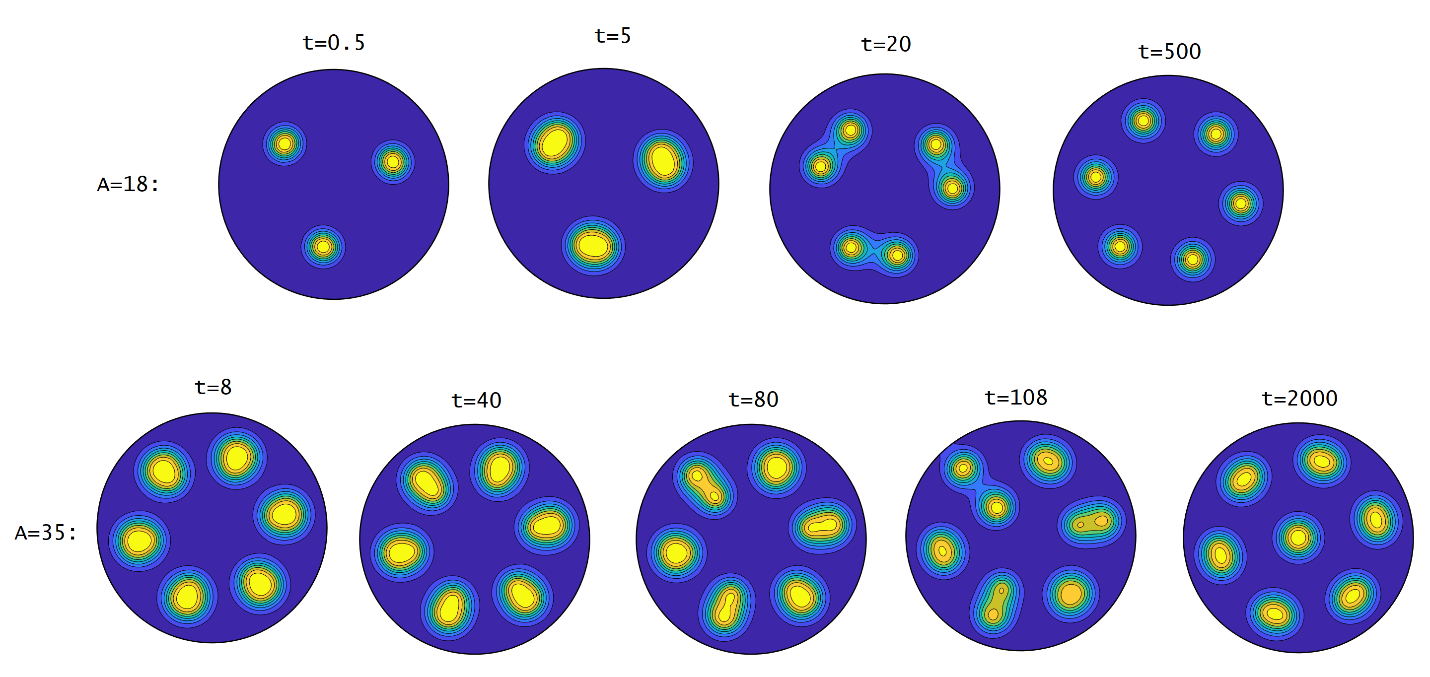
By contrast, Figure 3 shows a near-ring steady state of $N=8$ spikes. As we will see in §4, in the theoretical limit $\varepsilon\rightarrow 0$ and with $A$ sufficiently big, an 8-ring of spikes can be stable. However in practice, to stabilize such a ring, $\varepsilon$ needs to be taken too small to have accurate numerical 2D simulations (smaller than e.g. 0.01). With $\varepsilon=0.02$ our theory predicts $A_{l}=9.08$ and $A_{s}=52.90$ (c.f. Figure 2). But self-replication is observed above $A\approx 34.78$ (see equation (35) for a general formula), so we cannot take $A>52.9$ and still retain 8 spikes, since self-replication will result in more than 8 spots. In Figure 3, we took $A=16.7$. The result is a deformed ring of 8 spikes. In contrast to the 6-ring case, the deformation of an 8-ring appears to be supercritical, and leads to an 8-spike “square-type” configuration as shown in the figure.

For sufficiently large $A$, namely $A\gg O(\frac{N}{\log\varepsilon^{-1}}),$ it was shown in wei2008stationary that large eigenvalues are stable. In that case, the stability of small eigenvalues depends only on the number of spikes $N$ and the inner radius $b$ of annulus (assuming outer radius is 1). The following table gives the threshold value of $b_{c}(N)$ such that $N$ spikes are stable when $b>b_{c}(N):$

$N$ $\leq 8$ 9 10 11 12 13 14 15 16 17 18 19 20 $b_{c}(N)$ 0 0.174 0.293 0.356 0.412 0.450 0.488 0.516 0.545 0.567 0.589 0.607 0.625

(3)

Figure 4 shows a stable 10-spike ring configuration inside an annulus. Our analysis shows that a 10-spike configuration becomes unstable as $b$ is decreased below $b=0.293$ (see the table above) Indeed, the ring is observed to be stable for $b=0.35$ but unstable when $b=0.28.$ The instability is supercritical when $b$ is close to the threshold value and results in a zigzag-type configuration near the ring equilibrium radius.

We summarize this paper as follows. In section 2 we characterize the ring equilibrium radius, and more generally derive the reduced dynamics for $N$ spikes. This computation is relatively standard; see e.g. wei2008stationary; wong2020spot; kolokolnikov2020hexagonal; kolokolnikov2003reduced. In §3 we compute the stability with respect to large eigenvalues, specializing to the case of a spike ring. In §4 we linearize the reduced equations of motion to characterize the stability of a ring with respect to small eigenvalues. An important aspect of this paper are explicit computations with the Green’s functions and related functional for a disk or an annulus. These are performed in appendices. We conclude with some open problems in the §5.

In this section we derive the equilibium ring configuration of $N$ spikes, as well as reduced equations for spike dynamics. This is a relatively standard computation, see for example wei2008stationary; wong2020spot; ward2002dynamics; kolokolnikov2020hexagonal; kolokolnikov2003reduced; here, we follow kolokolnikov2020hexagonal. The ring of spikes is an equilibrium configuration for the reduced dynamics.

We start by deriving equations for reduced spike dynamics; these will subsequently be used to compute the ring radius and its stability with respect to small eigenvalues.

Inner region. We will assume that the spike centers $x_{k}$ move on a slow timescale of $O(\varepsilon^{2})$. This assumption will be seen to be self-consistent with asymptotic expansions below. As such, we start by expanding in the inner region near $k$-th spike

$$y=\frac{x-x_{k}(\varepsilon^{2}t)}{\varepsilon}.$$

(4)

Up to $O(\varepsilon^{2})$ terms, we expand:

	$\displaystyle u$	$\displaystyle=U_{0}(y)+\varepsilon U_{1}(y)+O(\varepsilon^{2});$
	$\displaystyle v$	$\displaystyle=V_{0}(y)+\varepsilon V_{1}(y)+O(\varepsilon^{2}).$

The equations for $U_{0},$ and $V_{0}$ become

	$\displaystyle 0$	$\displaystyle=\Delta_{y}U_{0}-U_{0}+U_{0}^{2}V_{0}$
	$\displaystyle 0$	$\displaystyle=\Delta_{y}V_{0}-\frac{1}{\log\varepsilon^{-1}}U_{0}^{2}V_{0}$

Next we expand in $\frac{1}{\log\varepsilon^{-1}}.$ Since we only need the leading order term, to leading order we have $\Delta_{y}V_{0}\sim 0$, so we approximate $V_{0}$ by a constant:

$$V_{0}\sim v_{k}=v(x_{k}).$$

The solution for $U_{0}$ is then given by

$$U_{0}(y)\sim\frac{w(y)}{v_{k}}$$

where $w$ is the ground state satisfying

$$\Delta w-w+w^{2}=0;\ \ \ w\text{ is radially symmetric; \ }w(y)\rightarrow 0\text{ as }\left|y\right|\rightarrow\infty.$$

(5)

The leading-order equations (in $\frac{1}{\log\varepsilon^{-1}}$) for $U_{1},V_{1}$ then become

	$\displaystyle-\frac{x_{k}^{\prime}(s)}{v_{k}}\nabla w$	$\displaystyle=\Delta U_{1}-U_{1}+2wU_{1}+w^{2}\frac{V_{1}}{v_{k}^{2}},$		(6)
	$\displaystyle\Delta V_{1}$	$\displaystyle=0.$		(7)

Multipying (6) by $\nabla w$ and integrating, we then obtain the equation for $x_{k}^{\prime}(s):$

$$-x_{k}^{\prime}(s)\int\left|\nabla w\right|^{2}=-\frac{1}{3v_{k}}\int w^{3}\nabla V_{1}$$

(8)

Outer region. To estimate the right hand side in (8), we compute the behaviour of $v$ in the outer region away from spike center. We estimate

$$v(x)\sim T-\sum_{j=1}^{N}S_{j}G(x,x_{j})$$

where $G(x,x_{j})$ is the Green’s function satisfying

$$\left\{\begin{array}[c]{l}\Delta G-\frac{1}{\pi}=-\delta(x-\xi),\ \ x,\xi\in\Omega_{b},\\ \partial_{n}G=0,\ \ x\in\partial\Omega_{b},\\ \int_{\Omega_{b}}G(x,\xi)dx=0\end{array}\right.$$

(9)

and $T,\ S_{j}$ satisfy

	$\displaystyle\frac{1}{v_{j}}\frac{1}{\log\varepsilon^{-1}}\int w^{2}dy$	$\displaystyle=S_{j};$
	$\displaystyle\sum S_{j}$	$\displaystyle=\left|\Omega\right|A.$

Recall that the Green’s function has the singularity structure,

$$G(x,x_{j})=-\frac{1}{2\pi}\log\left|x-x_{j}\right|+H\left(x,x_{j}\right).$$

Expanding the outer solution $v$ in the inner variables we then obtain an expansion

$$v(x_{k}+\varepsilon y)\sim T+S_{k}\frac{1}{2\pi}\log\left|y\right|-\sum_{j}S_{j}G_{kj}-\varepsilon y\cdot\sum_{j}S_{j}\nabla G_{kj}+O(\varepsilon^{2})$$

where

$$G_{kj}=\left\{\begin{array}[c]{c}G(x_{k},x_{j}),\ \ \ \ \text{if }k\neq j\\ \frac{1}{2\pi}\log\varepsilon^{-1}+H(x_{j},x_{j}),\text{ \ if }k=j\end{array}\right.,\ \ \ \ \ \nabla G_{kj}=\left\{\begin{array}[c]{c}\nabla_{x_{k}}G(x_{k},x_{j}),\ \ \ \ \text{if }k\neq j\\ \nabla_{x}H(x,\xi)|_{\begin{subarray}{c}x=x_{k}\\ \xi=x_{j}\end{subarray}},\text{ \ if }k=j\end{array}\right.$$

(10)

Matching with the inner expansion,

	$\displaystyle\nabla V_{10}$	$\displaystyle\sim-\sum_{j}S_{j}\nabla G_{kj};$
	$\displaystyle v_{k}$	$\displaystyle=T-\sum_{j}S_{j}G_{kj}$

Finally use the following identities identities, see for e.g. ward2002dynamics:

$$\frac{\int_{\mathbb{R}^{2}}w^{3}dy}{\int_{\mathbb{R}^{2}}w^{2}dy}=3,\ \ \ \ \frac{\int_{\mathbb{R}^{2}}\left|\nabla w\right|^{2}dy}{\int_{\mathbb{R}^{2}}w^{2}(y)dy}=1/2,\ \ \ \int_{\mathbb{R}^{2}}w^{2}dy\approx 31.04.$$

(11)

We summarize the spike dynamics as follows.

Ring equilibrium. In the case of a ring equilibrium with all spikes having identical heigth, we have that $S_{k}=S$ for all $k$, so that

$$S=S_{k}\sim\frac{\left|\Omega\right|A}{N}.$$

The ring equilibrium has the solution of the form

$$x_{k}=re^{2\pi ik/N}$$

We now define

$$J(r,R,l)=\left\{\begin{array}[c]{c}G(r,Re^{i2\pi l/N}),\ \ \ \ \text{if }l\neq 0\text{ (mod }N)\\ \frac{1}{2\pi}\log\varepsilon^{-1}+H(r,R),\text{ \ otherwise}\end{array}\right.$$

(13)

Then $R$ satisfies

$$\sum_{k=0}^{N-1}J_{r}(R,R,k)=0.$$

(14)

The function $J$ as well as the sum in (14) is computed using Fourier series decomposition in polar coordinates (see Appendix A). This yields the following equation for the ring radius $r:$

$$R^{2}-\frac{1}{2}+\frac{1}{2N}+\frac{1}{R^{-2N}-1}=0.$$

(15)

This equation was also derived in wong2020spot (equation (2.41)); in addition, the same equation describes an optimal radius kolokolnikov2005optimizing (equation (4.14)), in the context of optimizing the fundamental Neumann eigenvalue with $N$ small traps on a ring inside a unit disk.

It is easy to see that (15) has a unique root $R\in\left(0,1\right).$ The following table shows $R$ as a function of $N:$

	$$\displaystyle\text{Ring radius }R\text{ for a ring of }N\text{ spikes}$$
	$$\displaystyle\begin{array}[c]{cccccccccc}N&2&3&4&5&6&7&8&9&10\\ R&0.4536&0.5517&0.5985&0.6251&0.6417&0.6527&0.6604&0.6662&0.6706\end{array}$$

More generally, for an annulus $\left|x\right|\in\left(b,1\right),$ the calculations are relegated to Appendix B. As a result, we obtain the following expression for $R$ in terms of a rapidly converging series:

$$0=\frac{R^{2}-b^{2}}{\left(1-b^{2}\right)}-\frac{1}{2}+\frac{1}{2N}+\sum_{p=0}^{\infty}\left\{\frac{b^{2Np}}{R^{-2N}-b^{2Np}}-\frac{b^{2N(p+1)}}{R^{2N}-b^{2N(p+1)}}\right\}.$$

(18)

We now study the stability of a ring state with respect to large eigenvalues. We start by linearizing around the ring steady state as

$$u(x,t)=u(x)+\phi e^{\lambda t},\ \ \ v(x,t)=v(x)+\phi e^{\lambda t},\ \ \$$

to obtain the eigenvalue problem,

$$\lambda\phi=\varepsilon^{2}\Delta\phi-\phi+2uv\phi+u^{2}\psi,\ \ \ \ \Delta\psi-\left(2uv\phi+u^{2}\psi\right)\frac{1}{\varepsilon^{2}\log\varepsilon^{-1}}=0.$$

(19)

Near each spike location $x_{k}$ we let

$$x=x_{k}+\varepsilon y;\ \ \Phi_{k}(y)=\phi(x)\text{ \ and \ }\Psi_{k}=\psi\left(x_{k}\right).$$

Then we obtain the eigenvalue problem

$$\lambda\Phi_{k}=L_{0}\Phi_{k}+w^{2}\frac{\Psi_{k}}{v_{k}};\ \ \ \ \text{where }\ \ \ L_{0}\Phi:=\Delta\Phi-\Phi+2w\Phi.$$

(20)

We estimate

$$\Psi_{k}\sim C-\sum_{j}\left(\int\left(2w\Phi_{j}+w_{j}^{2}\frac{\Psi_{j}}{v_{j}^{2}}\right)dy\right)\frac{1}{\log\varepsilon^{-1}}G_{kj}$$

(21)

where $G_{kj}$ is given in (10); the constant $C$ is determined by integrating the equation for $\psi$ in (19) which results in

$$\sum_{k}\int\left(2w\Phi_{k}+w^{2}\frac{\Psi_{k}}{v_{k}^{2}}\right)dy=0.$$

(22)

Together, equations (20), (21) and (22) constitute an eigenvalue problem for $\lambda.$ Next, we specialize to the case of a ring spike state. The problem can be decoupled by introducing a circulant anzatz for the eigenfunction of the form

$$\Phi_{j}=z^{j}\Phi(y);\ \ \ \Psi_{j}=z^{j}\Psi;\ \ \ \ \ z:=\exp\left(2\pi mi/N\right),\ \ \ m=0\ldots N-1,\ \ \ C=0.$$

Then (20) becomes

$$\lambda\hat{\Phi}=L_{0}\hat{\Phi}+w^{2}\frac{\Psi}{v_{0}^{2}}.$$

Here, $v_{k}=v_{0}$ is the common height of all $N$ spikes, and $\Psi$ satisfies

$$\Psi\sim-\left(2\int w\Phi+\frac{\Psi}{v_{0}^{2}}\int w^{2}\right)\frac{1}{\log\varepsilon^{-1}}\sum_{l=0}^{N-1}z^{l}J.$$

(23)

Here and below, we abbreviate $J=J(R,R,l).$

We now study two cases separately, depending on whether $m=0$ or $m\neq 0.$

Case 1. $m=0.$ Then integrating the equation for $\Psi$ in (19) we obtain $\Psi=-\frac{\int 2w\Phi}{\int w^{2}}v_{0}^{2}$ and (20) becomes

$$\lambda\Phi=L_{0}\Phi-2w^{2}\frac{\int w\Phi}{\int w^{2}}.$$

(24)

This case is covered by Theorem 1.4 of wei1999single. For convenience, we state this theorem as follows.

Theorem (Wei, Theorem 1.4 of wei1999single) Consider the nonlinear eigenvalue problem

$$\lambda\Phi=L_{0}\Phi-\chi w^{2}\frac{\int w\Phi}{\int w^{2}}.$$

(25)

Suppose that $\chi>1.$ Then this problem is stable, that is, $\operatorname{Re}\left(\lambda\right)<0$. Suppose that $\chi<1.$ Then (25) admits a positive (i.e. unstable) eigenvalue $\lambda>0.$ When $\chi=1,$ (25) has a zero eigenvalue $\lambda=0$ corresponding to the eigenfunction $\Phi=w.$

It immediately follows that (24) is stable.

Case 2. $m\neq 0.$ Then (23) becomes (25) with

$$\chi=\frac{2}{1+\left(\frac{1}{\log\varepsilon^{-1}}\frac{\int w^{2}}{v_{0}^{2}}\sum_{l=0}^{N-1}z^{l}J\right)^{-1}}.$$

(26)

By Wei’s Theorem, the critical threshold is given when $\chi=1$, which yields

$$\frac{1}{\log\varepsilon^{-1}}\sum_{l=0}^{N-1}z^{l}J=\frac{v_{0}^{2}}{\int w^{2}}.$$

(27)

Note that $J(R,R,0)\sim\frac{1}{2\pi}\log\varepsilon^{-1}\gg O(1).$ We therefore define

$$\Upsilon\left(m\right):=\sum_{l=0}^{N-1}z^{l}J;\text{ \ and\ \ \ }\tilde{\Upsilon}:=\Upsilon-\frac{1}{2\pi}\log\varepsilon^{-1};$$

Replacing $v_{0}=\frac{1}{\log\varepsilon^{-1}}\frac{N\int w^{2}}{\left|\Omega\right|A}$ in (27) and solving for $A$ we then obtain the critical threshold for large eigenvalues $A_{l},$ given as

$$A_{l,m}=\frac{1}{\log\varepsilon^{-1}}\frac{N}{\left|\Omega\right|}\left(2\pi\int w^{2}\right)^{1/2}\left(1+\frac{2\pi}{\log\varepsilon^{-1}}\tilde{\Upsilon}(m)\right)^{-1/2}.$$

(28)

For values of $N\leq 8$ on a unit disk, the table below gives numerical values for $\tilde{\Upsilon}(m):$

N$\backslash$m 1 2 3 4 5 6 7 2 0.0509 3 0.0771 0.0771 4 0.148 -0.0406 0.148 5 0.233 -0.0579 -0.0579 0.233 6 0.325 -0.0495 -0.1129 -0.0495 0.325 7 0.4214 -0.0301 -0.131 -0.131 -0.0301 0.4214 8 0.5207 -0.00471 -0.1345 -0.164 -0.1345 -0.00471 0.5207

Note that in all cases, $\tilde{\Upsilon}(m)$ attains a minimum at $m=\left\lfloor N/2\right\rfloor.$ An explicit formula for $\tilde{\Upsilon}(m)$ with $N$ even and $m=N/2$ is available; it is given by:

$$\tilde{\Upsilon}(N/2)=\frac{1}{2\pi}\ln\left(\frac{4R}{N}\frac{1+R^{N}}{1-R^{N}}\right).$$

We now summarize our findings.

Note that to leading order, $A_{l}\sim A_{l,m}\sim A_{l0}$ as $\varepsilon\rightarrow 0,$ where

$$A_{l0}:=\frac{N}{\left|\Omega\right|}\frac{1}{\log\varepsilon^{-1}}\left(2\pi\int w^{2}\right)^{1/2}.$$

(31)

Indeed, this recovers the thresold computed in wei2008stationary for an arbitrary configuration of $N$ spikes. However in practice, the $\log\varepsilon$ correction makes a significant difference. Consider for example the case $N=8,$ $\varepsilon=0.05.$ Then formula (31) yields $A_{l0}=11.86$ whereas $A_{l}=14.66$, so that $O(1/\log\varepsilon)$ terms contribute about 25% increase to the instability threshold.

Small eigenvalues control the motion of the spikes. They can be computed by linearizing the reduced ODE (12) around its steady state. Numerical experiments indicate that the dominant small-eigenvalue instability of a ring results in a radial motion: half of the spikes move inside and half outside the ring. Thus, we make a simplifying assumption where $k-$th spike is restricted to move along a ray $\theta=2\pi k/N$. The restricted problem, up time-rescaling, becomes:

$$r_{k}^{\prime}=-S_{k}\sum_{l=0}^{N-1}S_{k+l}J_{r}(r_{k,}r_{k+l},l)\text{ \ with }\theta_{l}=2\pi l/N$$

with

$$\sum S_{k}=\left|\Omega\right|A,$$

$$\frac{1}{\log\varepsilon^{-1}}\frac{\int w^{2}}{S_{k}}=T-\sum_{l=0}^{N}S_{k+l}J(r_{k,}r_{k+l},l).$$

We now linearize around the equilibrium radius $r_{k}=R$ using circular Fourier series:

$$r_{k}=R+\phi z^{k}e^{\lambda t};\ \ \ \ S_{k}=S+\psi z^{k}e^{\lambda t};\ \ \ z=\exp\left(2\pi mi/N\right),\ \ \ m=0\ldots N$$

We then obtain:

	$\displaystyle\lambda\phi$	$\displaystyle=-\phi S^{2}\sum_{l=0}^{N-1}\left(J_{rr}+J_{rR}z^{l}\right)-\psi S\sum_{l=0}^{N-1}z^{l}J_{r},$
	$\displaystyle\frac{1}{\log\varepsilon^{-1}}\frac{\int w^{2}}{S^{2}}\psi$	$\displaystyle=\sum_{l=0}^{N-1}\psi z^{l}J+S\left(J_{r}+J_{R}z^{l}\right)\phi$

Here and below, $J$ denotes $J(R,R,l)$ as defined in (13), and we have used the fact that $\sum_{l=0}^{N-1}J_{r}=0$ for the equilibrium radius $R.$

Eliminating $\psi$ we obtain a single expression for the eigenvalue $\lambda:$

$$\frac{\lambda}{S^{2}}=-\sum_{l=0}^{N-1}\left(J_{rr}+J_{rR}z^{l}\right)-\frac{1}{\frac{1}{\log\varepsilon^{-1}}\frac{\int w^{2}}{S^{2}}-\sum_{l=0}^{N-1}z^{l}J}\left(\sum_{l=0}^{N-1}J_{r}z^{l}\right)^{2};$$

(32)

above we used the fact that $J(r,R,l)=J(R,r,l)$ so that $J_{R}(R,R)=J_{r}(R,R)$. Letting $\Upsilon(r,R,m)=\sum_{l=0}^{N-1}z^{l}J(r,R,l),$ we obtain

$$\frac{\lambda}{S^{2}}=-\Upsilon_{rr}(R,R,0)-\Upsilon_{rR}(R,R,m)-\frac{\Upsilon_{r}^{2}(R,R,m)}{\frac{\kappa}{S^{2}}-\Upsilon(R,R,m)}$$

Recall that

$$S=\frac{\left|\Omega\right|A}{N};\ \ \Upsilon=\frac{1}{2\pi}\log\varepsilon^{-1}+\tilde{\Upsilon}$$

where $\tilde{\Upsilon}$ is independent of $\varepsilon.$ It follows that in the limit $A\gg O(\frac{1}{\log\varepsilon^{-1}})$, the leading-order stability of small eigenvalues is determined by the sign of $\Upsilon_{rr}(R,R,0)+\Upsilon_{rR}(R,R,m).$ This quantity is equivalent to local minimizer condition of the Green’s functional from wei2008stationary, specialized to a ring of spikes. In addition, recall that $A_{l}=O(\frac{1}{\log\varepsilon^{-1}})$ so that $A\gg O(\frac{1}{\log\varepsilon^{-1}})$ automatically implies stability with respect to large eigenvalues. We summarize this as follows.

The following table lists the value of $\Lambda(m)$ on a unit disk, using formula (54):

$$\begin{array}[c]{c}\Lambda(m)\\ \begin{tabular}[c]{|l|l|l|l|l|l|l|l|l|l|}\hline\cr$N\backslash m$&1&2&3&4&5&6&7&8&9\\ \hline\cr 2&-0.7545&&&&&&&&\\ \hline\cr 3&-0.9955&-0.9955&&&&&&&\\ \hline\cr 4&-1.2006&-0.9851&-1.2006&&&&&&\\ \hline\cr 5&-1.3886&-0.9722&-0.9722&-1.3886&&&&&\\ \hline\cr 6&-1.5753&-0.9682&-0.7319&-0.9682&-1.5753&&&&\\ \hline\cr 7&-1.7699&-0.9795&-0.5129&-0.5129&-0.9795&-1.7699&&&\\ \hline\cr 8&-1.9750&-1.0074&-0.3213&-0.0825&-0.3213&-1.0074&-1.9750&&\\ \hline\cr 9&-2.1901&-1.0501&-0.1548&{0.3121}&{0.3121}&-0.1548&-1.0501&-2.1901&\\ \hline\cr 10&-2.4130&-1.1043&-0.0082&{0.6747}&{0.9036}&{0.6747}&-0.0082&-1.1043&-2.4130\\ \hline\cr\end{tabular}\end{array}$$

It shows that the dominant mode corresponds to $m=\left\lfloor N/2\right\rfloor;$ moreover a ring of $N\geq 9$ spikes is unstable for any $A.$

Note that condition $\Lambda<0$ alone does not guarantee ring stability when $A$ is of $O\left(\frac{1}{\log\varepsilon^{-1}}\right).$ The full stability characterisation is obtained by setting $\lambda=0$ in (32). Upon substituting $\lambda=0$ and $S=\frac{\left|\Omega\right|A}{N}$ in (32) and solving for $A,$ we obtain the following small-eigenvalue threshold which exists even when $\Lambda(m)<0$ for all $m\in\left(1,N\right):$

$$A_{s,m}=\frac{1}{\log\varepsilon^{-1}}\frac{N}{\left|\Omega\right|}\left(2\pi\int w^{2}\right)^{1/2}\left\{1+\frac{2\pi}{\log\varepsilon^{-1}}\left[\tilde{\Upsilon}(R,R,m)+\frac{\Upsilon_{r}^{2}(R,R,m)}{\Lambda(m)}\right]\right\}^{-1/2}.$$

(34)

Numerics show that the largest $A_{s,m}$ is attained when $m=\left\lfloor N/2\right\rfloor.$

Let us now contrast the small-eigenvalue threhsold $A_{s,m}$ in (34) with the the large-eigenvalue threshold $A_{l,m}$ in (28). Note that both $A_{s,m}$ and $A_{l,m}$ converge to $A_{l0}\sim\frac{1}{\log\varepsilon^{-1}}\frac{N}{\left|\Omega\right|}\left(2\pi\int w^{2}\right)^{1/2}$ as $\varepsilon\rightarrow 0$, which is independent of the mode $m.$ Moreover, suppose that $\Lambda(m)<0.$ (i.e. the ring is stable for sufficiently large $A$). Then $\frac{\Upsilon_{r}^{2}(R,R,m)}{\Lambda(m)}<0$ and it immediately follows from (34) and (28) that $A_{s}>A_{l}.$ We conclude that that small eigenvalues are destabilized before the big eigenvalues (although both thresholds agree at leading order). This is indeed the case whenever a ring is stable for sufficiently large $A$ (so that $\Lambda<0$). We summarize this as follows.

For a unit disk, this result applies to $N\leq 8$, since a ring of 9 or more spikes is unstable for any $A.$ More generally, (3) gives the radius $b_{c}(N)$ such that $N$ spikes are stable for large $A$ when $b>b_{c}(N).$ This table is generated by solving $\Lambda(\left\lfloor N/2\right\rfloor)=0$ for $b.$ Any number of spikes can be stabilized for sufficiently thin annulus. Deriving the exact asymptotics of this stabilization is an open question.

We have performed the stability analysis of a ring solution inside a unit disk or an annulus $\Omega_{b}=\left\{x:b\leq\left|x\right|\leq 1\right\}$. We found that there are two distinct mechanisms whereby a ring can undergo an instability. First, if $A$ is sufficiently large, the ring can be stabilized by making the annulus sufficiently thin. For a unit disk ($b=0$), the magic number is $N=8:$ less than 9 spikes are stable inside a disk assuming $A$ is sufficiently large (and $\varepsilon$ sufficiently small). Conversely, a ring of 9 or more spikes is unstable inside a unit disk but can be stabilized by increasing $b,$ as shown in (3). In fact, the thinner the annulus, the more spikes can be stable along the ring. It is an open question to work out the asymptotics for stability of a ring in the limit of thin annulus.

On the other hand, an $N-$ring can become unstable regardless of the $b$ if $A$ is decreased sufficiently. It was previously known that such an instability is triggered due to large eigenvalues when $A$ is decreased below $A_{l0}$ in (31). We have shown that there is also a small-eigenvalue instability $A_{s}$ just above $A_{l0}$ which triggers an instability. In particular for an $8-$ring on a disk, this small-eigenvalue instability explains the square-type pattern of 8 spikes observed (c.f. Figure 3). Numerics indicate that it is supercritical for an 8-ring on a unit disk but subcritical for a 6-spike ring. It is an open question to characterize the criticality analytically.

Another well-known instability for the Schnakenberg model is spike-replication, which occurs when $A$ is sufficiently increased. Following the analysis in kolokolnikov2009spot, it can be shown that self-replication of an $N$-ring occurs when $A$ is increased past $A_{r}$, where

$$A_{r}=\sqrt{\frac{1}{\log\varepsilon^{-1}}}\frac{N}{\left|\Omega_{b}\right|}4.3\cdot 2\pi.$$

(35)

Note that unlike competition thresholds $A_{l}$ and $A_{s}$, the formula for $A_{r}$ is independent of ring radius. This is due to the high symmetry (all heights being the same) of the ring. Figure 5 illustrates this phenomenon. Generally, the stability region is $A_{s}<A<A_{r}.$ For an 8-ring, we have $A_{s}\approx A_{r}\approx 33.8$ when $\varepsilon=0.016,$ and the ordering $A_{s}<A_{r}$ holds as long as $\varepsilon<0.016.$ In particular, no stable 8-ring can exist if $\varepsilon=0.02$ regardless of the choice of $A$ (c.f. as in figure 3).

Let us conclude with some open questions regarding ring self-replication. Figure 5 suggests that the direction of replication depends on the particular configuration. In the case of a 3-ring, the direction of self-replication is parallel to the boundary, whereas in the case of 6-ring, it is orthogonal to the boundary. Furthermore, number of spots that simulateneously self-replicate also varies with $N.$ For example, an “aborted” self-replication is observed in 2nd row of Figure 5: initially, all 6 spots exhibit self-replication instability; later on, only three of the six spots continue to replicate, but eventually only one spot succeeds in fully replicating. Further experiments (not shown) indicate that the number of self-replicating events is very sensitive to how much the feed rate $A$ is above the self-replication threshold $A_{r}$, as well as the total number of spots.

In this appendix we summarize the computations involving the Green’s function (9) on a unit disk $\Omega_{0}=\left\{x:\left|x\right|<1\right\}.$

Let $r=\left|x\right|,\ \ R=\left|\xi\right|,$ and let $\theta$ be the angle between $x,\xi.$ We decompose into Fourier series as follows:

$$G=\sum_{n=0}^{\infty}\cos(n\theta)g_{n}(r,R);\ \text{and}\ \ \delta(x-\xi)=\left(\frac{1}{2\pi}+\sum_{n=1}^{\infty}\frac{1}{\pi}\cos\left(n\theta\right)\right)\frac{\delta(r-R)}{r}$$

(36)

so that

	$\displaystyle\left(g_{n}\right)_{rr}+\frac{1}{r}\left(g_{n}\right)_{r}-n^{2}g_{n}$	$\displaystyle=-\frac{1}{\pi R}\delta(r-R),\ \ n\geq 1,$
	$\displaystyle\left(g_{0}\right)_{rr}+\frac{1}{r}\left(g_{0}\right)_{r}$	$\displaystyle=-\frac{1}{2\pi R}\delta(r-R),\ \ n=0.$

It is straighforward to verify that

	$\displaystyle g_{n}(r,R)$	$\displaystyle=\frac{1}{2\pi}\frac{1}{n}\left\{\begin{array}[c]{c}r^{n}\left(R^{n}+R^{-n}\right),\ \ \ r<R\\ R^{n}\left(r^{n}+r^{-n}\right),\ \ \ R<r<1\end{array}\right.,\ \ \ n\geq 1,$
	$\displaystyle g_{0}(r,R)$	$\displaystyle=\frac{1}{2\pi}\left\{\begin{array}[c]{c}\frac{r^{2}}{2}+C(R),\ \ \ r<R\\ \ln R-\ln r+\frac{r^{2}}{2}+C(R),\ \ \ R<r<1\end{array}\right..$

Here, $C(R)$ is determined via the integral constraint $\int G=0,$ which yields

$$C(R)=\frac{R^{2}}{2}-\log R-\frac{3}{4}.$$

(41)

Next, we need to compute the regular part $H=G+\frac{1}{2\pi}\log\left|x-\xi\right|.$ In what follows, we will assume without loss of generality that $r<R.$ We have the following expansion of the $\log\left|x-\xi\right|:$

$$\log\left|x-\xi\right|=\log R-\sum_{n=1}^{\infty}\cos(n\theta)\frac{r^{n}R^{-n}}{n},\ \ \ r<R$$

so that

$$2\pi H(r,R,\theta)=\frac{r^{2}}{2}+C(R)+\log R+\sum_{n=1}^{\infty}\cos(n\theta)\frac{1}{n}r^{n}R^{n}.$$

We remark that these formulas agree with an explicit expression for Green’s function given in ward2002dynamics, namely

	$\displaystyle G(x,\xi)$	$\displaystyle=-\frac{1}{2\pi}\log\left(\left|x-\xi\right|\right)+H(x,\xi);$		(42)
	$\displaystyle H(x,\xi)$	$\displaystyle=\frac{1}{4\pi}\left[-\log(\left|x\right|^{2}\left|\xi\right|^{2}+1-2x\cdot\xi)+\left|x\right|^{2}+\left|\xi\right|^{2}-\frac{3}{2}\right].$		(43)

References

• (1) J. Schnakenberg, Simple chemical reaction systems with limit cycle behaviour, Journal of theoretical biology 81 (3) (1979) 389–400.
• (2) S. Xie, T. Kolokolnikov, Moving and jumping spot in a two-dimensional reaction–diffusion model, Nonlinearity 30 (4) (2017) 1536.
• (3) J. Wei, M. Winter, Stationary multiple spots for reaction–diffusion systems, Journal of mathematical biology 57 (1) (2008) 53–89.
• (4) C. Muratov, V. Osipov, Spike autosolitons and pattern formation scenarios in the two-dimensional gray-scott model, The European Physical Journal B-Condensed Matter and Complex Systems 22 (2) (2001) 213–221.
• (5) M. J. Ward, J. Wei, The existence and stability of asymmetric spike patterns for the schnakenberg model, Studies in Applied Mathematics 109 (3) (2002) 229–264.
• (6) J. Wei, M. Winter, Existence and stability of multiple-spot solutions for the gray–scott model in r2, Physica D: Nonlinear Phenomena 176 (3-4) (2003) 147–180.
• (7) W. Chen, M. J. Ward, The stability and dynamics of localized spot patterns in the two-dimensional Gray-Scott model., SIAM J. Appl. Dynam. Systems, 2010.
• (8) T. Kolokolnikov, M. J. Ward, J. Wei, Spot self-replication and dynamics for the schnakenburg model in a two-dimensional domain, Journal of nonlinear science 19 (1) (2009) 1–56.
• (9) T. Wong, M. J. Ward, Spot patterns in the 2-d schnakenberg model with localized heterogeneities, arXiv preprint arXiv:2009.07882 (2020).
• (10) T. Kolokolnikov, F. Paquin-Lefebvre, M. J. Ward, Competition instabilities of spike patterns for the 1d gierer–meinhardt and schnakenberg models are subcritical, Nonlinearity 34 (1) (2021) 273.
• (11) T. Kolokolnikov, F. Paquin-Lefebvre, M. J. Ward, Stable asymmetric spike equilibria for the gierer–meinhardt model with a precursor field, IMA Journal of Applied Mathematics 85 (4) (2020) 605–634.
• (12) T. Kolokolnikov, J. Wei, Hexagonal spike clusters for some pde’s in 2d, Discrete & Continuous Dynamical Systems-B 25 (10) (2020) 4057.
• (13) T. Kolokolnikov, M. J. Ward, Reduced wave green’s functions and their effect on the dynamics of a spike for the gierer-meinhardt model, European Journal of Applied Mathematics 14 (5) (2003) 513–546.
• (14) M. J. Ward, D. McInerney, P. Houston, D. Gavaghan, P. Maini, The dynamics and pinning of a spike for a reaction-diffusion system, SIAM Journal on Applied Mathematics 62 (4) (2002) 1297–1328.
• (15) T. Kolokolnikov, M. S. Titcombe, M. J. Ward, Optimizing the fundamental neumann eigenvalue for the laplacian in a domain with small traps, European Journal of Applied Mathematics 16 (2) (2005) 161–200.
• (16) J. Wei, On single interior spike solutions of the gierer-meinhardt system: uniqueness and spectrum estimates, European Journal of Applied Mathematics 10 (4) (1999) 353–378.