Performing global sensitivity analysis on simulations of a continuous-time Markov chain model motivated by epidemiology

Consider a finite, closed (i.e. of constant size over time) population in which each individual has a health status (susceptible, infectious, and so on) evolving over time. The set of all possible health statuses is denoted by $\mathbf{V}$. Since those health statuses induce a partition of the whole population at any given time, the elements of $\mathbf{V}$ are also called compartments. Every time an individual changes compartments, we say that a transition occurs. Only certain types of transitions can occur. Let $\mathbf{E}$ denote the set of all possible types of transitions. By definition, for $\alpha,\beta\in\mathbf{V}$, an individual can move from $\alpha$ to $\beta$ if $(\alpha,\beta)\in\mathbf{E}$. The pair $(\mathbf{V},\mathbf{E})$ can be identified with a directed graph where $\mathbf{V}$ is the set of nodes and $\mathbf{E}$ is the set of arrows connecting the compartments between which the individuals can move. Assuming an ordering of the compartments has been chosen, let us identify the set $\mathbf{E}$ with a subset of $\mathbb{R}^{|\mathbf{V}|}$ as follows: with each $(\alpha,\beta)\in\mathbf{E}$, associate the vector of length $|\mathbf{V}|$ with components equal to zero except at the positions corresponding to $\alpha$ and $\beta$, where the components are $-1$ and $1$, respectively. The elements of $\mathbf{E}$ seen as a subset of $\mathbb{R}^{|\mathbf{V}|}$ are called transition vectors.

For every $\alpha\in\mathbf{V}$ and a vector of epidemic parameters $\theta\in\Theta\subset\mathbb{R}^{d}$, let $W^{\theta}_{\alpha}(t)$ be the number of individuals in compartment $\alpha$ at time $t$. Since the population is closed, we have that $\sum_{\alpha\in\mathbf{V}}W^{\theta}_{\alpha}(t)$ is constant over time. Denote by $W^{\theta}=(W_{\alpha}^{\theta})_{\alpha\in\mathbf{V}}$ the stochastic process that describes the whole population over time. It is assumed that $W^{\theta}$ is a continuous-time Markov chain with state space $\mathcal{E}\subset\mathbb{N}^{|\mathbf{V}|}$ and positive rate functions $g_{\mathbf{u}}(\theta,\xi)$, $\mathbf{u}\in\mathbf{E}$, $\xi\in\mathcal{E}$, given by

The initial state $W^{\theta}(0)=:\xi_{0}\in\mathcal{E}$ is supposed to be fixed. A description of the CTMC of the classical SIR model is given in Example 1.

In this section, we first recall the definition of variance-based Sobol’ sensitivity indices introduced in Sobol’ 1993 for deterministic models with scalar output. Following the paradigm of GSA, we model uncertain inputs by a random vector of independent components $\mathbf{X}=(X_{1},\dots,X_{m})$. Let $E_{1},\dots,E_{m}$ be subsets of $\mathbb{R}$ and $f_{1}\,:\,E_{1}\times\ldots\times E_{m}\rightarrow\mathbb{R}$ be some function such that $\mathbb{E}\left(f_{1}(\mathbf{X})^{2}\right)<+\infty$. Then first-order and total Sobol’ indices (see, e.g., Sobol’ 1993; Homma and Saltelli 1996) of the ouput $Y=f_{1}(\mathbf{X})$ associated with input $X_{j},j=1,\cdots,m$, are respectively defined as:

The definition of first-order and total Sobol’ indices can be extended to models with vectorial or functional output (see, e.g., Lamboni et al. 2011; Gamboa et al. 2014). Let ${\color[rgb]{0,0,0}Y=(Y_{1},\ldots,Y_{p})}:=f_{2}(X_{1},\ldots,X_{m})$ be a vectorial output where $f_{2}\,:\,\,E_{1}\times\ldots\times E_{m}\rightarrow\mathbb{R}^{p}$ is some function and $\mathbb{E}\left(\|Y\|^{2}\right)<+\infty$, with $\|\cdot\|$ denoting the Euclidean norm on $\mathbb{R}^{p}$. Aggregated first-order and total Sobol’ indices are defined as:

where $S_{X_{j},k}$ and $S_{X_{j},k}^{\textup{tot}}$ are the first-order and total Sobol’ indices of the scalar output $Y_{k}$ associated with the input $X_{j}$, for $k=1,\ldots,p$ and $j=1,\ldots,m$. If the output of the model of interest is a function of time, it can be reduced to a vectorial output through discretization of time. Then aggregated first-order and total Sobol’ indices can be computed using (3) and (4), where the output components $Y_{k}$ would be the values of the function at the time points of the discretization. Also first-order and total indices defined in Equations (1) and (2) can be computed at each time point of the discretization in order to obtain dynamics of Sobol’ indices.

Let $Y^{\theta}$ denote the random output of some stochastic model with parameters $\theta\in\Theta\subset\mathbb{R}^{d}$. For instance, $Y^{\theta}$ might be the stochastic process $W^{\theta}$ introduced in Section 2.1, or any scalar (or vectorial) quantity of interest defined as a functional of the process $W^{\theta}$. Note that distinct values of the parameters encoded in $\theta$ correspond to distinct epidemiological patterns. We thus consider the collection $\{Y^{\theta}\,,\;\theta\in\Theta\}$ and assume mutual independence between its members.

As in Section 2.2, uncertain parameters are modeled by a random vector $\mathbf{X}=(X_{1},\dots,X_{d})$ with independent components. In addition, it is assumed that $\mathbf{X}$ is independent of $\{Y^{\theta}\,,\;\theta\in\Theta\}$. The pair $(\mathbf{X},Y^{\mathbf{X}})$ represents the input/output pair that an external observer would see should they draw uncertain parameters at random. The object $Y^{\theta}$ is then the output observed conditionally on $\mathbf{X}=\theta$.

It is important to note that in $Y^{\mathbf{X}}$ there are two sources of variability (and hence uncertainty): the one coming from the uncertainty of the parameters (that is, modeled by vector $\mathbf{X}$), and the one coming from the intrinsic randomness of the stochastic model (that is, for a fixed $\theta$ the variability in $Y^{\theta}$). A complete GSA aims at separating these two sources of uncertainty and quantifying interactions between both.

To achieve this aim, it is necessary to control the latent variables modeling intrinsic randomness. More precisely, we aim at finding a function $f$ and a latent or a set of latent variables $Z$, independent of $\mathbf{X}$, such that the probability distributions of $Y^{\theta}$ and $f(\theta,Z)$ coincide. Since $\mathbf{X}$ is independent of $Z$ and $Y^{\theta}$, we immediately have that the input/output pairs $(\mathbf{X},Y^{\mathbf{X}})$ and $(\mathbf{X},f(\mathbf{X},Z))$ are equal in distribution. The pair $(f,Z)$ is called a deterministic representation (or simply a representation) of the stochastic model $Y^{\theta}$. Often, the function $f$ is the function induced by a (deterministic) algorithm which, if the inputs of that algorithm were drawn from the right distribution, would produce an output statistically equal to the given stochastic model.

From the viewpoint of GSA, one advantage of constructing a deterministic representation of a stochastic model is that standard methods of GSA for deterministic models can be applied straightforwardly. For instance, we can compute first-order and total Sobol’ indices by letting $m=d+1$ and $X_{d+1}=Z$ in (1) and (2) (or in (3) and (4) if the output is vectorial or functional).

In general, there is no unique deterministic representation of a stochastic model. The set of latent variables modeling intrinsic randomness $Z$ and the function $f$ may vary from one representation to the other. More precisely, if $Y^{\theta}$ is a stochastic model and $(f,Z)$ a representation of it, there may exist another representation $(\tilde{f},\tilde{Z})$ of $Y^{\theta}$ such that the laws of $(\mathbf{X},\tilde{f}(\mathbf{X},\tilde{Z}))$ and $(\mathbf{X},f(\mathbf{X},Z))$ coincide. (Here the probability distribution of $\tilde{Z}$ may be different from that of $Z$.) An example of a toy stochastic model with two different representations is provided in Example 2 below.

As different representations can be exhibited for a same stochastic model, we can wonder how the choice of representations affects GSA results. Let us consider $(f,Z)$ and $(\tilde{f},\tilde{Z})$ two distinct representations of a same stochastic model with uncertain parameters $\mathbf{X}=\left(X_{1},\cdots,X_{d}\right)$ and output $Y^{\mathbf{X}}$. We say that an index $S_{X_{j}}$ is representation free if $S_{X_{j}}(f,Z)=S_{X_{j}}(\tilde{f},\tilde{Z})$, where here $S_{X_{j}}(f,Z)$ and $S_{X_{j}}(\tilde{f},\tilde{Z})$ denote the values of the index $S_{X_{j}}$ based on the representations $(f,Z)$ and $(\tilde{f},\tilde{Z})$, respectively.

To show that Proposition 3 is true, it suffices to exhibit an example where two distinct representations lead to distinct first-order Sobol’ indices associated with intrinsic randomness and distinct total Sobol’ indices associated with uncertain parameters. Before giving the example, let us give some intuition behind Proposition 3. Note that the random variables $\displaystyle\mathbb{E}\left[f(\mathbf{X},Z)\mid(\mathbf{X}_{-j},Z)\right]$ and $\displaystyle\mathbb{E}\left[\tilde{f}(\mathbf{X},\tilde{Z})\mid(\mathbf{X}_{-j},\tilde{Z})\right]$ have different probability distributions in general. Indeed, since $(f,Z)\neq(\tilde{f},\tilde{Z})$, the way each function $f$ or $\tilde{f}$ combines its (set of) latent variable(s) $Z$ with input $X_{j}$ to generate the output may differ. Thus there is no reason for total Sobol’ indices associated with uncertain parameters to be representation free. Also, there is no reason for the random variables $\mathbb{E}\left[f(\mathbf{X},Z)\mid Z\right]$ and $\mathbb{E}\left[\tilde{f}(\mathbf{X},\tilde{Z})\mid\tilde{Z}\right]$ to have the same probability distributions and hence the first-order Sobol’ index associated with intrinsic randomness to be representation free. This is illustrated on the toy Example 3 below.

We conclude from this section that intrinsic randomness can be modeled in different manners. GSA results naturally depend on the modeling choice. Different modelings bring different insights. We discuss this point further on a SARS-CoV-2 spread model in Section 5. In the following section, we exhibit different meaningful representations for CTMC stochastic compartmental models, based on different simulation algorithms.

Recall from Section 2 that each process $W^{\theta}_{\alpha}$, $\alpha\in\mathbf{V}$, counts the number of individuals in compartment $\alpha$ over time. In this section we let $\mathbf{V}=\{S,E,A,I,H,R,D\}$, where the seven compartments represent seven possible health statuses: an individual can be susceptible (S), exposed (E) (i.e. infected but not yet infectious), asymptomatic infectious (A), symptomatic infectious (I), hospitalized (H), recovered (R) or dead (D). There are nine possible types of transition between these compartments, see Figure 1. Note that infection is neglected within hospitals so that hospitalized individuals cannot infect. Moreover, it is assumed that recovered individuals get perfectly immunized so they cannot be susceptible after recovering. The vector of uncertain parameters is given by $\theta=\left(\beta,\gamma_{E},\gamma_{A},\gamma_{I},\gamma_{H},p_{(E,A)},p_{C},p_{D|C},p_{(H,D)}\right)$. The different types of transition and their characteristics (transition vector $\mathbf{u}$ and associated rate function $g_{\mathbf{u}}$) are described in Table 1.

The list of uncertain epidemic parameters is given in Table 2. Instead of parameterizing the transitions from $I$ to $R$, $H$ or $D$ with the probabilities $p_{IR}$, $p_{IH}$ and $p_{ID}$, that correspond to the probability for an individual in $I$ to recover, to be hospitalized or to die, that are clearly not independent as $p_{IH}+p_{ID}+p_{IR}=1$, we chose to use instead parameters $p_{C}$ corresponding to the probability for an individual in compartment $I$ of being in a critical state and $p_{D|C}$ corresponding to the probability to die without being hospitalized conditionally on being in a critical state. These last two parameters are considered as independent from each other. This re-parameterization was inspired, e.g., from what is done in (Da Veiga et al. 2021, Chapter 7, page 191). More generally all the parameters listed in Table 2 are assumed to be independent. The nominal value and range of variation for each parameter has been chosen in agreement with current knowledge and represent at least plausible values; see, e.g., (Knock et al. 2021, Table S2 on page 15 of the Supplementary Material) and, specifically for parameters $p_{C}$ and $p_{D|C}$, (Da Veiga et al. 2021, Chapter 7).

We consider a population of $N=2005$ individuals including five exposed individuals at the start of the epidemic $t=0$, so that the process $W^{\theta}$ has the initial state

We focus on two quantities of interest (QoIs). First we consider a scalar QoI, namely the extinction time $Y^{\theta}_{ext}$ of the epidemic, defined as the first instant at which there are no exposed (E) nor infectious (A or I) individuals anymore:

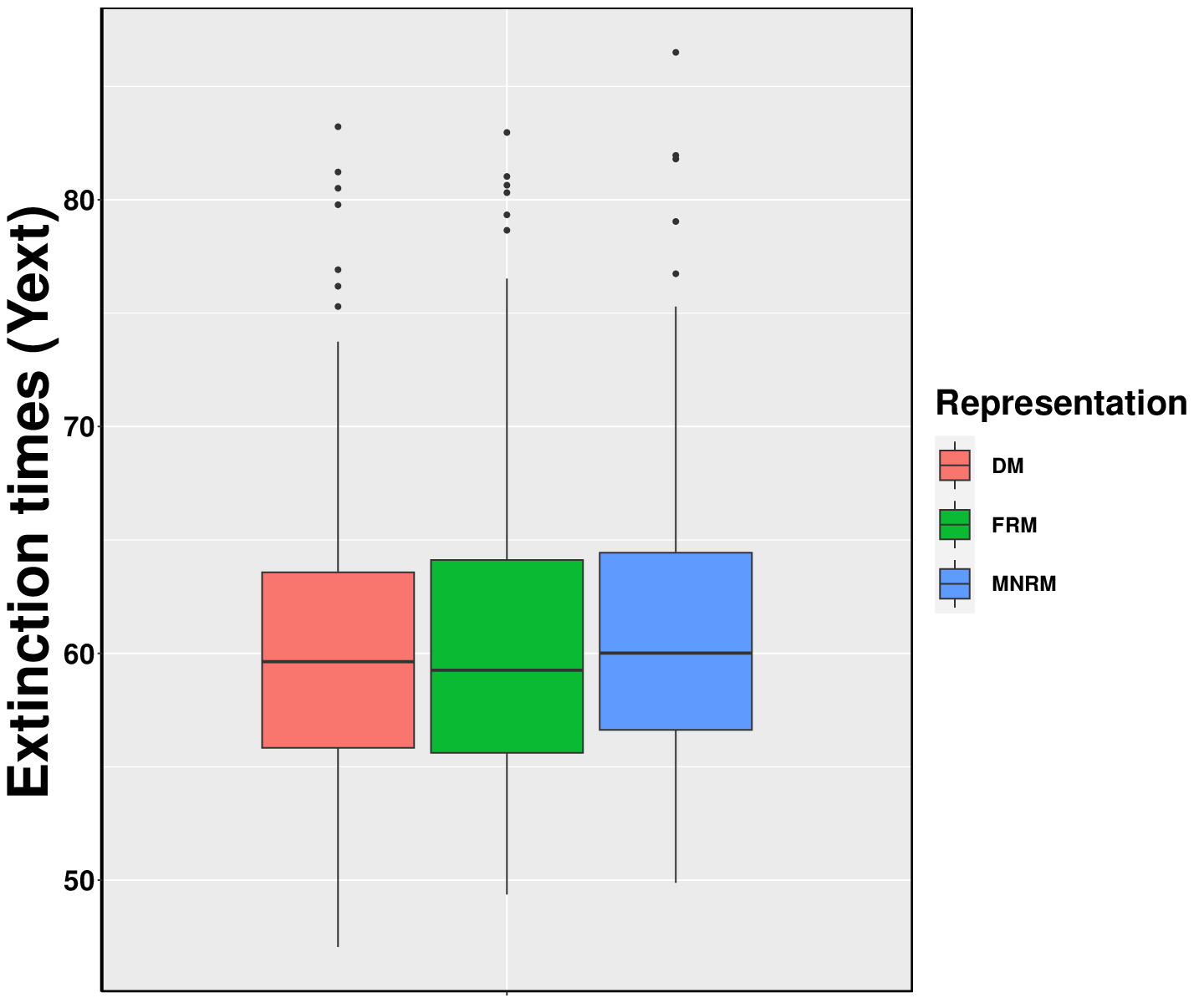
Note that for all $\theta\in\Theta$, $Y^{\theta}_{ext}$ is well-defined, i.e. $Y^{\theta}_{ext}<+\infty$. Indeed, by considering the compartmental model described in Figure 1, after a finite number of transitions, the stochastic process will necessarily reach an absorbing state with empty compartments $E,A$ and $I$. We display in Figure 2 two hundred independent realizations of $Y_{ext}^{\theta}$ for each of the simulation algorithms of Section 4. The uncertain parameters $\theta$ were set to the nominal values given in Table 2. The three boxplots are similar, which was expected since the distributions of the processes returned by each of the three algorithms are the same.

The second QoI we are considering is the dynamic of the number of symptomatic infectious individuals:

where $t_{\mathrm{end}}$ was set to 60. (The process dies out at around that time, see Figure 3.) We display in Figure 3 twenty independent realizations of the process $Y_{I}^{\theta}$ for each of the simulation algorithms of Section 4. The input parameter vector $\theta$ was set to the nominal values given in Table 2. The three charts in Figure 3 display similar sample paths for $Y_{I}^{\theta}$, which was expected since the distribution of the processes returned by each of the three algorithms is the same.

In the top row of Figure 3, we show $20$ independent trajectories of the process $t\mapsto W_{I}^{\theta}(t)$, obtained from Gillespie Direct Method (left), Gillespie First Reaction Method (middle) and Modified Next Reaction Method (right) with the components of the parameter vector $\theta$ fixed to their nominal value (see Table 2). On the bottom row of the same figure, we show the evolution over time of quantiles of different order (from $0.1$ to $0.9$) calculated from $1000$ independent trajectories of each algorithm (from left to right). These plots are in coherence with the fact that Algorithms 1, 2 and 3 are all exact simulation algorithms of the same stochastic process.

In practice, simulations are carried out using the R Statistical Software (R Core Team 2021). Sensitivity indices are estimated by using the R package sensitivity (Iooss et al. 2021). The function soboljansen() is used for total Sobol’ index estimation while sobol2007() is used for first-order Sobol’ index estimation. A priori distributions for model parameters are uniform distributions as described in Table 2 and the a priori for intrinsic randomness is modeled by seeds uniformly distributed in $\{1,\cdots,10^{9}\}$. Sensitivity indices are estimated from two independent designs of $n=2000$ input-output samples, where for each sample a trajectory of $W^{\theta}$ is simulated through either Algorithm 1, Algorithm 2 or Algorithm 3. As the dimension of the input space is large (at least $7$ model parameters plus inputs modeling intrinsic randomness whose number depends on the simulation algorithm), we use Latin Hypercube Sampling (see, e.g., Lin and Tang 2015). Latin Hypercube Samples are generated by using the R package DiceDesign (Dupuy et al. 2015).

This section is devoted to the presentation and comparison of sensitivity analysis results obtained for the algorithms presented in Section 4, namely Gillespie Direct Method, Gillespie First Reaction Method and Modified Next Reaction Method. In Section 5.3.1 we present the results for the scalar output of interest, namely the extinction time of the epidemy $Y_{ext}^{\theta}$. Then in Section 5.3.2 we present the sensitivity analysis results for the functional output corresponding to the dynamic of the number of symptomatic infectious individuals $Y_{I}^{\theta}$. Finally in Section 5.4 we discuss the choice of algorithms, depending on the practitioner’s objectives. Recall that in all the results presented in this section, sensitivity indices were estimated from two independent designs of $n=2000$ input-output samples, and the estimation was repeated independently $50$ times for the different boxplots.

The numerical experiments confirm that the sensitivity analysis results depend on the choice of the simulation algorithm. An interesting conclusion is that Gillespie algorithms are less prone to interactions between uncertain parameters and intrinsic randomness. It implies that simulations with Gillespie algorithms are more robust to a local perturbation of uncertain input parameters as we can see below by perturbing parameter $\beta$.

To plot Figure 10, we first simulate, for each simulation algorithm (Gillespie Direct Method, Gillespie First Reaction, Modified Next Reaction), $2\,000$ trajectories (corresponding to $2\,000$ different seeds) of the difference between the number of symptomatic infectious individuals computed with all uncertain parameters fixed to their nominal value and the number of symptomatic infectious individuals computed by perturbing only parameter $\beta$ by $5\,\%$ from its nominal value. Then in Figure 10 are plotted highest density region (HDR) boxplots. It is clear on these plots that the small perturbation applied to parameter $\beta$ has a much stronger impact when Modified Next Reaction Method is used for simulations. We thus expect that quantities calculated from a Monte-Carlo sampling scheme are less robust to an inaccurate estimate of parameter $\beta$ when using simulations based on Modifed Next Reaction Algorithm.

References

- Anderson [2007] D. F. Anderson. A modified next reaction method for simulating chemical systems with time dependent propensities and delays. The Journal of Chemical Physics, 127(21):214107, 2007. doi: 10.1063/1.2799998.
- Bittihn and Golestanian [2020] P. Bittihn and R. Golestanian. Stochastic effects on the dynamics of an epidemic due to population subdivision. Chaos: An Interdisciplinary Journal of Nonlinear Science, 30(10):101–102, Oct. 2020. ISSN 1054-1500. doi: 10.1063/5.0028972.
- Brauer [2008] F. Brauer. Compartmental Models in Epidemiology, pages 19–79. Springer Berlin Heidelberg, Berlin, Heidelberg, 2008. ISBN 978-3-540-78911-6. doi: 10.1007/978-3-540-78911-6_2.
- Britton [2009] T. Britton. Stochastic epidemic models: a survey. Mathematical biosciences, 225 1:24–35, 2009.
- Cazelles et al. [2021] B. Cazelles, C. Champagne, B. Nguyen-Van-Yen, C. Comiskey, E. Vergu, and B. Roche. A mechanistic and data-driven reconstruction of the time-varying reproduction number: Application to the covid-19 epidemic. PLOS Computational Biology, 17(7):1–20, 07 2021. doi: 10.1371/journal.pcbi.1009211.
- Courcoul et al. [2011] A. Courcoul, H. Monod, M. Nielen, D. Klinkenberg, L. Hogerwerf, F. Beaudeau, and E. Vergu. Modelling the effect of heterogeneity of shedding on the within herd coxiella burnetii spread and identification of key parameters by sensitivity analysis. Journal of Theoretical Biology, 284(1):130–141, 2011. ISSN 0022-5193. doi: https://doi.org/10.1016/j.jtbi.2011.06.017.
- Cristancho Fajardo et al. [2021] L. Cristancho Fajardo, P. Ezanno, and E. Vergu. Accounting for farmers’ control decisions in a model of pathogen spread through animal trade. Scientific Reports, 11(1):9581, May 2021. ISSN 2045-2322. doi: 10.1038/s41598-021-88471-6.
- Da Veiga et al. [2021] S. Da Veiga, F. Gamboa, B. Iooss, and C. Prieur. Basics and trends in sensitivity analysis: Theory and practice in R. SIAM, 2021.
- Dupuy et al. [2015] D. Dupuy, C. Helbert, and J. Franco. DiceDesign and DiceEval: Two R packages for design and analysis of computer experiments. Journal of Statistical Software, 65(11):1–38, 2015.
- Ethier and Kurtz [1986] S. N. Ethier and T. G. Kurtz. Markov processes – characterization and convergence, chapter 4, 6. Wiley Series in Probability and Mathematical Statistics: Probability and Mathematical Statistics. John Wiley & Sons Inc., New York, 1986. ISBN 0-471-08186-8.
- Étoré et al. [2020] P. Étoré, C. Prieur, D. K. Pham, and L. Li. Global sensitivity analysis for models described by stochastic differential equations. Methodology and Computing in Applied Probability, 22(2):803–831, June 2020. ISSN 1387-5841, 1573-7713. doi: 10.1007/s11009-019-09732-6.
- Fort et al. [2021] J.-C. Fort, T. Klein, and A. Lagnoux. Global sensitivity analysis and Wasserstein spaces. SIAM/ASA Journal on Uncertainty Quantification, 9(2):880–921, 2021. doi: 10.1137/20M1354957.
- Gamboa et al. [2014] F. Gamboa, A. Janon, T. Klein, and A. Lagnoux. Sensitivity analysis for multidimensional and functional outputs. Electronic Journal of Statistics, 8(1):575 – 603, 2014. doi: 10.1214/14-EJS895.
- Gillespie [1976] D. T. Gillespie. A general method for numerically simulating the stochastic time evolution of coupled chemical reactions. Journal of Computational Physics, 22(4):403–434, 1976. ISSN 0021-9991. doi: https://doi.org/10.1016/0021-9991(76)90041-3.
- Goel et al. [2023] S. Goel, S. K. Bhatia, J. P. Tripathi, S. Bugalia, M. Rana, and V. P. Bajiya. SIRC epidemic model with cross-immunity and multiple time delays. Journal of Mathematical Biology, 87(3):42, 2023.
- Hanthanan Arachchilage et al. [2023] K. Hanthanan Arachchilage, M. Y. Hussaini, N. Cogan, and M. H. Cortez. Exploring how ecological and epidemiological processes shape multi-host disease dynamics using global sensitivity analysis. Journal of Mathematical Biology, 86(5):83, 2023.
- Hart et al. [2017] J. L. Hart, A. Alexanderian, and P. A. Gremaud. Efficient computation of Sobol’ indices for stochastic models. SIAM Journal on Scientific Computing, 39(4):A1514–A1530, 2017. doi: 10.1137/16M106193X.
- Homma and Saltelli [1996] T. Homma and A. Saltelli. Importance measures in global sensitivity analysis of nonlinear models. Reliability Engineering and System Safety, 52(1):1–17, 1996. ISSN 0951-8320. doi: https://doi.org/10.1016/0951-8320(96)00002-6.
- Hyndman [1996] R. J. Hyndman. Computing and graphing highest density regions. The American Statistician, 50(2):120–126, 1996.
- Hyndman and Shang [2010] R. J. Hyndman and H. L. Shang. Rainbow plots, bagplots, and boxplots for functional data. Journal of Computational and Graphical Statistics, 19(1):29–45, 2010.
- Iooss et al. [2021] B. Iooss, S. Da Veiga, A. Janon, and G. Pujol. sensitivity: Global Sensitivity Analysis of Model Outputs, 2021. URL https://CRAN.R-project.org/package=sensitivity. R package version 1.24.0.
- Jimenez et al. [2017] M. N. Jimenez, O. P. Le Maître, and O. M. Knio. Nonintrusive polynomial chaos expansions for sensitivity analysis in stochastic differential equations. SIAM/ASA Journal on Uncertainty Quantification, 5(1):378–402, Jan. 2017. ISSN 2166-2525. doi: 10.1137/16M1061989.
- Karlin and Taylor [1981] S. Karlin and H. M. Taylor. A second course on stochastic processes. Academic Press, 1981.
- Knock et al. [2021] E. S. Knock, L. K. Whittles, J. A. Lees, P. N. Perez-Guzman, R. Verity, R. G. FitzJohn, K. A. M. Gaythorpe, N. Imai, W. Hinsley, L. C. Okell, A. Rosello, N. Kantas, C. E. Walters, S. Bhatia, O. J. Watson, C. Whittaker, L. Cattarino, A. Boonyasiri, B. A. Djaafara, K. Fraser, H. Fu, H. Wang, X. Xi, C. A. Donnelly, E. Jauneikaite, D. J. Laydon, P. J. White, A. C. Ghani, N. M. Ferguson, A. Cori, and M. Baguelin. Key epidemiological drivers and impact of interventions in the 2020 sars-cov-2 epidemic in england. Science Translational Medicine, 13(602):42–62, 2021. doi: 10.1126/scitranslmed.abg4262.
- Kurtz [1982] T. G. Kurtz. Representation and approximation of counting processes. In W. H. Fleming and L. G. Gorostiza, editors, Advances in Filtering and Optimal Stochastic Control, pages 177–191, Berlin, Heidelberg, 1982. Springer Berlin Heidelberg. ISBN 978-3-540-39517-1.
- Lamboni et al. [2011] M. Lamboni, M. Hervé, and M. David. Multivariate sensitivity analysis to measure global contribution of input factors in dynamic models. Reliability Engineering and System Safety, 96(4):450 – 459, 2011. ISSN 0951-8320. doi: https://doi.org/10.1016/j.ress.2010.12.002.
- Le Maître and Knio [2015] O. Le Maître and O. Knio. PC analysis of stochastic differential equations driven by wiener noise. Reliability Engineering & System Safety, 135:107–124, 2015. ISSN 0951-8320. doi: https://doi.org/10.1016/j.ress.2014.11.002.
- Le Maître et al. [2015] O. P. Le Maître, O. M. Knio, and A. Moraes. Variance decomposition in stochastic simulators. The Journal of Chemical Physics, 142(24):244115, 2015. doi: 10.1063/1.4922922.
- Lin and Tang [2015] C. Lin and B. Tang. Latin hypercubes and space-filling designs. In A. Dean, M. Morris, J. Stufken, and D. Bingham, editors, Handbook of design and analysis of experiments, Handbooks of modern statistical methods. Chapman & Hall/CRC, 2015.
- Marino et al. [2008] S. Marino, I. B. Hogue, C. J. Ray, and D. E. Kirschner. A methodology for performing global uncertainty and sensitivity analysis in systems biology. Journal of Theoretical Biology, 254(1):178–196, 2008. ISSN 0022-5193. doi: https://doi.org/10.1016/j.jtbi.2008.04.011. URL https://www.sciencedirect.com/science/article/pii/S0022519308001896.
- Marrel et al. [2012] A. Marrel, B. Iooss, S. Da Veiga, and M. Ribatet. Global sensitivity analysis of stochastic computer models with joint metamodels. Statistics and Computing, 22(3):833–847, May 2012. ISSN 1573-1375. doi: 10.1007/s11222-011-9274-8.
- Massard et al. [2022] M. Massard, R. Eftimie, A. Perasso, and B. Saussereau. A multi-strain epidemic model for covid-19 with infected and asymptomatic cases: Application to french data. Journal of Theoretical Biology, 545:111117, 2022. ISSN 0022-5193. doi: https://doi.org/10.1016/j.jtbi.2022.111117. URL https://www.sciencedirect.com/science/article/pii/S0022519322001151.
- Mazo [2021] G. Mazo. A trade-off between explorations and repetitions for estimators of two global sensitivity indices in stochastic models induced by probability measures. SIAM/ASA Journal on Uncertainty Quantification, 9(4):1673–1713, 2021. doi: 10.1137/19M1272706.
- Navarro Jimenez et al. [2016] M. Navarro Jimenez, O. P. Le Maître, and O. M. Knio. Global sensitivity analysis in stochastic simulators of uncertain reaction networks. The Journal of Chemical Physics, 145(24):244106, 2016. doi: 10.1063/1.4971797.
- Ngonghala et al. [2015] C. N. Ngonghala, M. I. Teboh-Ewungkem, and G. A. Ngwa. Persistent oscillations and backward bifurcation in a malaria model with varying human and mosquito populations: implications for control. Journal of mathematical biology, 70(7):1581–1622, 2015.
- R Core Team [2021] R Core Team. R: A Language and Environment for Statistical Computing. R Foundation for Statistical Computing, Vienna, Austria, 2021. URL https://www.R-project.org/.
- Richard et al. [2021] Q. Richard, S. Alizon, M. Choisy, M. T. Sofonea, and R. Djidjou-Demasse. Age-structured non-pharmaceutical interventions for optimal control of covid-19 epidemic. PLOS Computational Biology, 17(3):1–25, 03 2021. doi: 10.1371/journal.pcbi.1008776.
- Rimbaud et al. [2018] L. Rimbaud, C. Bruchou, S. Dallot, D. R. J. Pleydell, E. Jacquot, S. Soubeyrand, and G. Thébaud. Using sensitivity analysis to identify key factors for the propagation of a plant epidemic. Royal Society Open Science, 5(1):171435, 2018. doi: 10.1098/rsos.171435.
- Saltelli et al. [2000] A. Saltelli, K. Chan, and E. M. Scott. Sensitivity Analysis. John Wiley & Sons, 2000.
- Sellke [1983] T. Sellke. On the asymptotic distribution of the size of a stochastic epidemic. Journal of Applied Probability, 20(2):390–394, 1983. doi: 10.2307/3213811.
- Sobol’ [1993] I. M. Sobol’. Sensitivity analysis for non-linear mathematical models. Mathematical Modelling and Computational Experiment, 1:407–414, 1993.
- Torii et al. [2023] A. J. Torii, R. Begnini, H. M. Kroetz, O. M. I. Matar, R. H. Lopez, and L. F. F. Miguel. Global sensitivity analysis for mathematical models comparison. Computational and Applied Mathematics, 42(8):345, 2023.
- Veiga [2021] S. D. Veiga. Kernel-based ANOVA decomposition and shapley effects – application to global sensitivity analysis, 2021. arXiv:2101.05487.
- Williams and Rasmussen [2006] C. K. Williams and C. E. Rasmussen. Gaussian processes for machine learning, volume 2. MIT press Cambridge, MA, 2006.
- Yang et al. [2016] J. Yang, Y. Chen, and F. Xu. Effect of infection age on an SIS epidemic model on complex networks. Journal of mathematical biology, 73:1227–1249, 2016.
- Zhu and Sudret [2021] X. Zhu and B. Sudret. Global sensitivity analysis for stochastic simulators based on generalized lambda surrogate models. Reliability Engineering & System Safety, 214:107815, 2021. ISSN 0951-8320. doi: https://doi.org/10.1016/j.ress.2021.107815.
- Zhu and Sudret [2023] X. Zhu and B. Sudret. Stochastic polynomial chaos expansions to emulate stochastic simulators. International Journal for Uncertainty Quantification, 13(2):31–52, 2023. ISSN 2152-5080.