Validation and Improvement of the Pan-STARRS Photometric Calibration with the Stellar Color Regression Method
Abstract
As one of the best ground-based photometric dataset, Pan-STARRS1 (PS1) has been widely used as the reference to calibrate other surveys. In this work, we present an independent validation and re-calibration of the PS1 photometry using spectroscopic data from the LAMOST DR7 and photometric data from the corrected Gaia EDR3 with the Stellar Color Regression (SCR) method. Using per band typically a total of 1.5 million LAMOST-PS1-Gaia stars as standards, we show that the PS1 photometric calibration precisions in the filters are around mmag when averaged over regions. However, significant large- and small-scale spatial variation of magnitude offset, up to over 1 per cent, probably caused by the calibration errors in the PS1, are found for all the filters. The calibration errors in different filters are un-correlated, and are slightly larger for the and filters. We also detect moderate magnitude-dependent errors (0.005, 0.005, 0.005, 0.004, 0.003 mag per magnitude in the 14 – 17 magnitude range for the filters, respectively) in the PS1 photometry by comparing with the Gaia EDR3 and other catalogs. The errors are likely caused by the systematic uncertainties in the PSF magnitudes. We provide two-dimensional maps to correct for such magnitude offsets in the LAMOST footprint at different spatial resolutions from to . The results demonstrate the power of the SCR method in improving the calibration precision of wide-field surveys when combined with the LAMOST spectroscopy and Gaia photometry.
Keywords:
Astronomy data analysis, Stellar photometry, Calibrationsubmitted to AJ \submittedReceived: 2021 December 28; Revised: 2022 February 08; Accepted: 2022 February 09
I Introduction
The current and next-generation wide-field imaging surveys such as the Sloan Digital Sky Survey (SDSS; York et al. 2000), the Panoramic Survey Telescope and Rapid Response System (Pan-STARRS; Kaiser et al. 2002), the Dark Energy Survey (DES; Flaugher et al. 2015; Dark Energy Survey Collaboration et al. 2016; Abbott et al. 2018), the Javalambre Physics of the Accelerating Universe Astrophysical Survey (J-PAS; Benitez et al. 2014), the Wide Field Survey Telescope (WFST; Lou et al. 2016), the Chinese Space Station Telescope (CSST; Zhan 2018), the Legacy Survey of Space and Time (LSST; Ivezić et al. 2019) and the Multi-channel Photometric Survey Telescope (Mephisto; Er et al. 2021, in preparation), are vital in modern astronomy in discovering and characterizing new objects and phenomena. While uniform and accurate photometric calibration play a central role in the wide-field surveys.
Recently, some new approaches have been developed for the high-precision calibration of wide field surveys. The methods can be divided into categories of either: “hardware-driven” or “software-driven” (Huang & Yuan 2022). Approaches of the former category are based on better understanding of the wide-field imaging observations, and include such as the Ubercalibration method (Padmanabhan et al. 2008), the Forward Global Calibration Method (FGCM; Burke et al. 2018), and the Hypercalibration method (Finkbeiner et al. 2016); while those of the latter category are based on better understanding of stellar colors, such as the Stellar Locus Regression method (SLR; High et al. 2009), the Stellar Locus method (SL; López-Sanjuan et al. 2019), and the Stellar Color Regression method (SCR; Yuan et al. 2015).
Owing to the rapid development of multi-fiber spectroscopic surveys, e.g., LAMOST (Deng et al. 2012; Liu et al. 2014), we have entered into the era of millions of stellar spectra. In addition, with the modern template-matching and data-driven based stellar parameter pipelines (e.g., Lee et al. 2008a; Lee et al. 2008b; Wu et al. 2011; Xiang et al. 2015; Xiang et al. 2017), stellar atmospheric parameters, such as , , , can be determined to a very high internal precision (e.g., Niu et al. 2021a). As a result, stellar colors can now be accurately predicted based on the large-scale spectroscopic surveys. Using millions of spectroscopically observed stars as color standards, Yuan et al. 2015 first proposed the spectroscopy-based SCR method and performed precise color (re-)calibrations for the SDSS Stripe 82. Compared to the other “software-driven” methods, the SCR method fully accounts the effects of metallicity, surface gravity, and dust reddening on stellar colors. When applied to the SDSS Stripe 82 (Ivezić et al. 2007), it achieved a precision of 2 – 5 mmag in the SDSS colors. The method has also been applied to the Gaia Data Release 2 and Early Data Release 3 (EDR3) to correct for the magnitude/color-dependent systematic errors in the Gaia colors (Niu et al. 2021a; Niu et al. 2021b), achieving an unprecedented precision of 1 mmag. Together with the high-precision photometry from Gaia, the SCR method can further be used to predict stellar magnitudes accurately and perform photometric calibration. For example, Huang et al. 2021 have applied the method to recalibrate the DR2 of the SkyMapper Southern Survey (SMSS; Wolf et al. 2018), and find large zero-point offsets in the bands. Huang & Yuan 2022 have applied the method to the SDSS Stripe 82 standard stars catalogs (Ivezić et al. 2007; Thanjavur et al. 2021), achieving a precision of 5 mmag in the band, and 2 mmag in the bands. Possible implementations of the SCR method under different situations and improvements are also discussed by Huang & Yuan 2022.
As the first part of the Pan-STARRS (Kaiser et al. 2002; Kaiser et al. 2010), Pan-STARRS1 (PS1; Tonry et al. 2012) has imaged three quarters of the sky repeatly in five broadband filters (, , , , ). Taking advantage of the large amount of over-lapping observations, PS1 photometry has been calibrated using the ubercalibration method to a precision better than 1 per cent (Schlafly et al. 2012; Magnier et al. 2020). As one of the best ground-based photometric dataset, PS1 has been widely used as reference to calibrate other surveys, including the SDSS survey (Finkbeiner et al. 2016), the Beijing–Arizona Sky Survey (BASS; Zou et al. 2017; Zhou et al. 2018), the J-PLUS (López-Sanjuan et al. 2019; López-Sanjuan et al. 2021). It has also been used as cross-calibration of multiple photometric systems to improve the cosmological measurements with Type Ia supernovae (see Scolnic et al. 2015; Brout et al. 2021).
In this work, using the SCR method with the corrected photometric data from the Gaia EDR3 (Yang et al. 2021) and the spectroscopic date from LAMOST DR7, validation and improvement of the PS1 photometric calibration are performed. The paper is organized as follows. In Sections II and III, we introduce the data used and the validation process with the SCR method in this work. The results are presented in Section IV and discussed in Section V. Conclusions are given in Section VI.
II Data
II.1 Pan-STARRS 1 Data Release 1
The PS1 survey has imaged three quarters of the sky in five broadband filters (, , , , ), using its 1.8 meter telescope of a field of view (Hodapp et al. 2004) and 1.4 Gigapixel camera. Its first public data release (DR1) on 16 December 2016 contains the results of the third full reduction of the Pan-STARRS Survey (Magnier et al. 2020). The typical limiting magnitudes for point sources are (23.3, 23.2, 23.1, 22.3, 21.4) in the (, , , , ) bands, respectively (Chambers et al. 2016). PSF magnitudes, Kron magnitudes, and aperture magnitudes are provided in the PS1 DR1. PSF magnitudes are obtained from fitting a predefined PSF model using maximum-likelihood methods, and mainly for stars. Kron magnitudes are mainly for extended sources. Aperture magnitudes measure the total flux for a point source based on integration over an aperture plus an extrapolation according to the PSF. In this work, PSF magnitudes are used as default.
II.2 Gaia Early Data Release 3
The EDR3 (Gaia Collaboration et al. 2021a; Gaia Collaboration et al. 2021b) of the European Space Agency (ESA)’s space mission Gaia (Gaia Collaboration et al. 2016) has delivered not only the best astrometric information but also the best photometric data for about 1.8 billion stars in , and bands, in terms of full sky coverage, uniform calibration at mmag level, and small photometric errors for a very wide range of magnitudes. The overall calibration errors are less than 1 mmag for overall trend except for very blue and bright sources (Riello et al. 2021). More recently, Yang et al. 2021 carried out an independent validation of Gaia EDR3 photometry against about 10,000 Landolt standard stars using a machine-learning technique. They obtained magnitude-dependent corrections up to 10 mmag for the three Gaia bands. Hence, Gaia EDR3 magnitudes hereafter refer to those corrected by Yang et al. 2021.
II.3 LAMOST Data Release 7
The Large Sky Area Multi-Object Fiber Spectroscopic Telescope (LAMOST; Cui et al. 2012; Zhao et al. 2012; Deng et al. 2012; Liu et al. 2014) is a quasi-meridian reflecting Schmidt telescope with 4000 fibers, and has a field of view of 20 deg2. Its Data Release 7 (hereafter DR7; see Luo et al. 2015) includes a total number of 10,640,255 low resolution spectra covering the whole optical wavelength range of 369 – 910 nm at a spectral resolution of about 1800. The LAMOST Stellar Parameter Pipeline (LASP; Wu et al. 2011) has been used to determine the basic stellar parameters including effective temperature , surface gravity and metallicity . The typical precision is about 110 K for , 0.2 dex for , and 0.1 dex for (Luo et al. 2015).
III Validation process with the SCR method
;


An overview of the validation process using the SCR method to the PS1 calibration is shown in Figure 1. The details are as below:
- a.
Combine the PS1 DR1 photometric data with the Gaia EDR3 and the LAMOST DR7. The adopted cross-matching radius is .
- b.
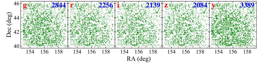
Select main sequence stars () as the calibration samples with the following constraints: 1) mag{} 14 and mag{} 13 to avoid saturation; 2) error{} 0.02 mag; 3) phot_bp_rp_excess_factor to avoid bad Gaia photometry; 4) K, a relatively narrow temperature range for robust fitting of intrinsic colors with atmospheric parameters and the temperature-dependence reddening coefficients, but still with sufficient numbers of stars; 5) for an easy intrinsic color fitting with atmospheric parameters; and 6) Signal-to-noise ratio for the band () of the LAMOST spectra . Finally, 1,688,097, 1,299,006, 1,162,825, 1,113,294 and 1,931,225 stars are selected in the , , , and bands, respectively. The calibration sample in the band is shown in Figure 2 and 3. Then, the control sample stars are selected as those within a small and low-extinction area (). A total number of 2844, 2256, 2139, 2084 and 3389 control stars are selected for the bands, respectively. Their spatial distributions are shown in Figure 4.
For reddening correction, the dust reddening map of Schlegel et al. 1998 is not used as it fails at low Galactic latitudes and shows spatially-dependent systematic errors (Sun et al., submitted). In this work, the values of obtained with the star-pair method (Yuan et al. 2013; Ruoyi & Haibo 2020) are adopted instead.
- c.
Five colors are adopted for the bands, where and . Then, for the control sample, a 2nd-order two-dimensional polynomial (with 6 free parameters, see Equation (1)) as a function of and is used to fit the intrinsic colors (). Here the intrinsic colors are estimated using Equation (2), where represents reddening coefficients.
(1) (2) where
- d.
Moderate magnitude-dependent residuals are found when fitting intrinsic colors as a function of and of the control samples in each band. Therefore, we use a linear polynomial, , to fit the residuals (). To account for magnitude-dependent errors in the PS1 data, corrected magnitudes are obtained by . Then, we put the corrected magnitudes into the previous step (Figure 1(c)). Iterations are performed.
- e.
Based on the results from the above two steps, intrinsic colors are obtained for the calibration stars, so are their reddening values . Then, the reddening coefficients with respect to are derived by linear regression with clipping. Note that the lines are not forced to pass through the origin. The non-zero offsets, , represent the zero-point differences between the control samples and the calibration samples. Iterations are also needed here, as shown in Figure 1. Finally, mag.
In this process, because of the very broad passbands of and , we have also considered the influence of temperature on the reddening coefficients. Temperature-dependent reddening coefficients are adopted for the and colors.
- f.

| Intrinsic Color | Constant Term | |||||
|---|---|---|---|---|---|---|

| Color | Constant | |||
|---|---|---|---|---|


| Slope () | Constant () | |
|---|---|---|


IV Results


The final fitting results of the intrinsic colors as a function of (, ) are shown in Figure 5. The corresponding fitting parameters are listed in Table 1. The fitting residuals are respectively 0.0097, 0.0080, 0.0067, 0.0067 and 0.0106 mag for the , , , and colors, suggesting that one can predict PS1 magnitudes to a precision of 1 per cent or better from the LAMOST and Gaia data for individual stars. The fitting residuals show no dependence on and , and magnitude either after correcting the magnitude-dependent errors. The final fitting coefficients of magnitude-dependence corrections are listed in Table 3. The slopes imply that magnitude-dependent corrections are 0.005, 0.005, 0.005, 0.004, 0.003 mag per magnitude in the 14 – 17 magnitude range for the bands, respectively. Note that the magnitude-dependent corrections are relative. The corrections are zero at () = (15.1, 15.1, 15.2, 15.2, 14.3), which are the typical magnitudes of the control samples.
The results of reddening coefficients with respect to in the five colors are plotted in Figure 6. It can be seen that the reddening coefficients show moderate dependence on stellar temperature for the and colors. Therefore, taking 500 K as the bin width, the calibration stars are divided into 16 overlapping bins according to their temperature. Reddening coefficients of the 16 bins are further obtained via linear regression, with the same offset. Then, we use a cubic polynomial of 4 free parameters to fit the reddening coefficients as a function of . The final fitting parameters are given in Table 2. The temperature dependence of reddening coefficients for the , and colors are very weak and ignored. Their fitting coefficients are given in Figure 6.
Figure 7 shows the spatial variations of magnitude offsets after binning with a window for the , , , and bands. We can see both large-scale and small-scale patterns for all the five bands. The small-scale patterns, having a typical size similar to the PS1 field-of-view (3.3 degree), is more clearly displayed in Figure 8 for the band. The same mottling also appears in Figure 10 of Magnier et al. 2020. The large-scale patterns are different between different bands. The band shows the strongest patterns, probably due to the strong and variable water absorption of the atmosphere. The spatial patterns suggest that the magnitude offsets are caused by calibration errors in the PS1 rather than Gaia.
To investigate whether the derived magnitude offsets are affected by possible systematic errors in reddening correction, the correlations between the magnitude offsets of different bands are calculated and shown in Figure 9. The correlation coefficients are very close to zero, suggesting that systematic errors in reddening correction are very small. However, we note that the magnitude offsets of two bands can show clear correlations in certain sky areas.
To quantitatively estimate calibration errors of the PS1 data, we plot the magnitude offsets as a function of star numbers in one box in Figure 11. The standard deviations are also estimated using Gaussian fitting. The values decrease as the star numbers increases first, then become flat when the star numbers are larger than 10. The convergence values are respectively 4.6, 3.9, 3.5, 3.6, and 4.8 mmag for the , , , and bands, confirming that the PS1 data has achieved an internal precision of mag (Schlafly et al. 2012).
To correct the above patterns, we perform an adaptive median smoothing. The initial box size is . If the star numbers within a box is less than 20, then the box size is doubled until it reaches to . The results of the five bands after smoothing are plotted in Figure 10, and can be used to correct calibration errors in the PS1 data within the LAMOST footprint. The data is publicly available11 1 http://paperdata.china-vo.org/Xiao.Kai/PS1/spatial_corr.zip. The corrected magnitude can be computed as
| (5) |
where is the observed magnitude, is the position-dependent magnitude offset (see Figure 10), and is the magnitude-dependent magnitude offset (see Table 3). To check the effect of correction, we over-plot the magnitude offsets after correction as a function of star numbers in Figure 11. The standard deviations decrease to 0.4 – 0.5 mmag for the five bands.
We also apply our corrected magnitudes of PS1 back to the linear regression process of reddening coefficients. All the fitting residuals are smaller, decreasing from 9.5 to 8.3, 9.1 to 8.2, 7.4 to 6.8, 8.1 to 7.3, and 11.0 to 9.5 mmag for the bands, respectively. These numbers are consistent with those in Figure 11. For example, 4.6.
V Discussions
After correcting for the magnitude-dependent errors, we plot variation of magnitude offsets with magnitudes and color of the calibration samples in Figure 12. As expected, no dependence on magnitudes is found. The dependence on is also ignorable.
To further verify the magnitude-dependent corrections, we perform an independent check using data from the re-calibrated SDSS Stripe 82 standard stars catalog (V4.2; Huang & Yuan 2022) and DES DR1. Stars within a sub-stripe of and are used. All these stars are in the high Galactic latitude region and suffer very low extinction. First, we construct different color-color relations, e.g., versus , and use them to obtain the predicted PS1 magnitudes from the SDSS/DES magnitudes and colors. Note that the filter differences between different surveys are corrected here via color-color relations. Then we plot the offsets between the predicted and observed PS1 magnitudes as a function of PS1 magnitude. An example of the magnitude offset in band from the SDSS Stripe 82 varying with is shown in Figure 13. The results are summarized in Figure 14. Note that the results from the SDSS and DES are shifted slightly in the vertical direction for easy comparison.
Figure 14 shows that for the , , and bands, both the results of SDSS stripe 82 and DES DR1 agree well with our corrections from Gaia EDR3 for magnitudes between 14 – 17. For the band, our corrections are consistent with those of DES DR1 only. For the band, only result from the DES DR1 is obtained, with a much deeper slope. The results suggest that the moderate magnitude-dependent errors in the PS1 magnitudes are real.
To investigate the possible causes of the magnitude-dependent errors, we select 20,000 stars from PS1 DR1 and compare their aperture-based and PSF magnitudes. Note that all the magnitudes mentioned earlier refer to the PSF magnitudes in this work. The results are plotted in Figure 15. These results are also plotted in Figure 14 with green dots for comparison, after shifting of the zero points. Figure 14 suggests that our corrections from Gaia EDR3 agree with the differences between the aperture-based and PSF magnitudes in each band. It implies that most of the magnitude-dependent errors in the PS1 PSF magnitudes probably come from systematic errors in the PSF magnitudes. Note that the uncertainties in the non-linearity corrections of the CCDs may also contribute partly.
Portillo et al. 2020 noted that the PSF photometry using maximum-likelihood methods systematically overestimate the flux, with a bias scaling with the inverse signal-to-noise ratio and the number of model parameters involved in the fit. One expects a 1 per cent bias for a 10 point source and 0.01 per cent bias for a 100 point source. Given the brightness of the calibration stars used in this work, such effect may contribute only a small fraction to the systematic errors in the PS1 PSF magnitudes.
VI Conclusions
In this paper, using the SCR method with the photometric data from the corrected Gaia EDR3 and the spectroscopic data from LAMOST DR7, we have performed an independent validation and recalibration of the PS1 photometry. Using typically a total of 1.5 million LAMOST-PS1-Gaia FGK dwarf stars as standards per band, we show that the PS1 photometric calibration precisions are respectively 4.6, 3.9, 3.5, 3.6, and 4.8 mmag in the bands when averaged over regions. However, significant large- and small-scale spatial variation of magnitude offsets, up to over 1 per cent and caused by calibration errors in the PS1, are found for all the filters. The calibration errors in different filters are un-correlated in most sky areas. The band shows the strongest patterns, probably due to the strong and variable water absorption of the atmosphere.
We also detect the moderate magnitude-dependent errors in the PS1 photometry, i.e., 0.005, 0.005, 0.005, 0.004, 0.003 mag per magnitude in the 14 – 17 magnitude range for the filters, respectively. Such errors are further confirmed by comparing the PS1 magnitudes with those predicted from the re-calibrated SDSS Stripe 82 standard stars catalog (V4.2) and DES DR1. Such errors are likely caused by systematic uncertainties in the PSF magnitudes.
It implies that most of the magnitude-dependent errors in the PS1 PSF magnitudes probably come from systematic errors in the PSF magnitudes. Note that the uncertainties in the non-linearity corrections of the CCDs may also contribute partly.
We provide two-dimensional maps to correct for position-dependent magnitude offsets in the LAMOST footprint at resolutions from to . The maps, together with the magnitude-dependent corrections, are useful in the usage of the PS1 photometry for high-precision investigations (e.g., Niu et al. 2021c; Xu et al. 2021) and as the reference to calibrate other surveys.
The results demonstrate the power of the SCR method in improving calibration precision of wide-field surveys when combined with Gaia photometry. We suggest that the SCR method should be incorporated into the calibration process of future releases of the PS1 data.
References
- Abbott et al. (2018) Abbott, T. M. C., Abdalla, F. B., Allam, S., et al. 2018, ApJS, 239, 18. doi:10.3847/1538-4365/aae9f0
- Benitez et al. (2014) Benitez, N., Dupke, R., Moles, M., et al. 2014, arXiv:1403.5237
- Brout et al. (2021) Brout, D., Taylor, G., Scolnic, D., et al. 2021, arXiv:2112.03864
- Burke et al. (2018) Burke, D. L., Rykoff, E. S., Allam, S., et al. 2018, AJ, 155, 41. doi:10.3847/1538-3881/aa9f22
- Chambers et al. (2016) Chambers, K. C., Magnier, E. A., Metcalfe, N., et al. 2016, arXiv:1612.05560
- Cui et al. (2012) Cui, X.-Q., Zhao, Y.-H., Chu, Y.-Q., et al. 2012, Research in Astronomy and Astrophysics, 12, 1197. doi:10.1088/1674-4527/12/9/003
- Dark Energy Survey Collaboration et al. (2016) Dark Energy Survey Collaboration, Abbott, T., Abdalla, F. B., et al. 2016, MNRAS, 460, 1270. doi:10.1093/mnras/stw641
- Deng et al. (2012) Deng, L.-C., Newberg, H. J., Liu, C., et al. 2012, Research in Astronomy and Astrophysics, 12, 735. doi:10.1088/1674-4527/12/7/003
- Finkbeiner et al. (2016) Finkbeiner, D. P., Schlafly, E. F., Schlegel, D. J., et al. 2016, ApJ, 822, 66. doi:10.3847/0004-637X/822/2/66
- Flaugher et al. (2015) Flaugher, B., Diehl, H. T., Honscheid, K., et al. 2015, AJ, 150, 150. doi:10.1088/0004-6256/150/5/150
- Gaia Collaboration et al. (2016) Gaia Collaboration, Prusti, T., de Bruijne, J. H. J., et al. 2016, A&A, 595, A1. doi:10.1051/0004-6361/201629272
- Gaia Collaboration et al. (2021a) Gaia Collaboration, Brown, A. G. A., Vallenari, A., et al. 2021a, A&A, 649, A1. doi:10.1051/0004-6361/202039657
- Gaia Collaboration et al. (2021b) Gaia Collaboration, Brown, A. G. A., Vallenari, A., et al. 2021b, A&A, 650, C3. doi:10.1051/0004-6361/202039657e
- High et al. (2009) High, F. W., Stubbs, C. W., Rest, A., et al. 2009, AJ, 138, 110. doi:10.1088/0004-6256/138/1/110
- Huang & Yuan (2022) Huang, B. & Yuan, H. 2022, ApJS, in press
- Huang et al. (2021) Huang, Y., Beers, T. C., Wolf, C., et al. 2021, arXiv:2104.14154
- Huang et al. (2021) Huang, Y., Yuan, H., Li, C., et al. 2021, ApJ, 907, 68. doi:10.3847/1538-4357/abca37
- Hodapp et al. (2004) Hodapp, K. W., Kaiser, N., Aussel, H., et al. 2004, Astronomische Nachrichten, 325, 636. doi:10.1002/asna.200410300
- Ivezić et al. (2007) Ivezić, Ž., Smith, J. A., Miknaitis, G., et al. 2007, AJ, 134, 973. doi:10.1086/519976
- Ivezić et al. (2019) Ivezić, Ž., Kahn, S. M., Tyson, J. A., et al. 2019, ApJ, 873, 111. doi:10.3847/1538-4357/ab042c
- Kaiser et al. (2002) Kaiser, N., Aussel, H., Burke, B. E., et al. 2002, Proc. SPIE, 4836, 154. doi:10.1117/12.457365
- Kaiser et al. (2010) Kaiser, N., Burgett, W., Chambers, K., et al. 2010, Proc. SPIE, 7733, 77330E. doi:10.1117/12.859188
- Lee et al. (2008a) Lee, Y. S., Beers, T. C., Sivarani, T., et al. 2008a, AJ, 136, 2022. doi:10.1088/0004-6256/136/5/2022
- Lee et al. (2008b) Lee, Y. S., Beers, T. C., Sivarani, T., et al. 2008b, AJ, 136, 2050. doi:10.1088/0004-6256/136/5/2050
- Liu et al. (2014) Liu, X.-W., Yuan, H.-B., Huo, Z.-Y., et al. 2014, Setting the scene for Gaia and LAMOST, 298, 310. doi:10.1017/S1743921313006510
- Lou et al. (2016) Lou, Z., Liang, M., Yao, D., et al. 2016, Proc. SPIE, 10154, 101542A. doi:10.1117/12.2248371
- López-Sanjuan et al. (2019) López-Sanjuan, C., Varela, J., Cristóbal-Hornillos, D., et al. 2019, A&A, 631, A119. doi:10.1051/0004-6361/201936405
- López-Sanjuan et al. (2021) López-Sanjuan, C., Yuan, H., Vázquez Ramió, H., et al. 2021, A&A, 654, A61. doi:10.1051/0004-6361/202140444
- Luo et al. (2015) Luo, A.-L., Zhao, Y.-H., Zhao, G., et al. 2015, Research in Astronomy and Astrophysics, 15, 1095. doi:10.1088/1674-4527/15/8/002
- Magnier et al. (2020) Magnier, E. A., Schlafly, E. F., Finkbeiner, D. P., et al. 2020, ApJS, 251, 6. doi:10.3847/1538-4365/abb82a
- Niu et al. (2021a) Niu, Z., Yuan, H., & Liu, J. 2021a, ApJ, 909, 48. doi:10.3847/1538-4357/abdbac
- Niu et al. (2021b) Niu, Z., Yuan, H., & Liu, J. 2021b, ApJ, 908, L14. doi:10.3847/2041-8213/abe1c2
- Niu et al. (2021c) Niu, Z., Yuan, H., Wang, S., et al. 2021c, ApJ, 922, 211. doi:10.3847/1538-4357/ac2573
- Padmanabhan et al. (2008) Padmanabhan, N., Schlegel, D. J., Finkbeiner, D. P., et al. 2008, ApJ, 674, 1217. doi:10.1086/524677
- Portillo et al. (2020) Portillo, S. K. N., Speagle, J. S., & Finkbeiner, D. P. 2020, AJ, 159, 165. doi:10.3847/1538-3881/ab76ba
- Riello et al. (2021) Riello, M., De Angeli, F., Evans, D. W., et al. 2021, A&A, 649, A3. doi:10.1051/0004-6361/202039587
- Ruoyi & Haibo (2020) Ruoyi, Z. & Haibo, Y. 2020, ApJ, 905, L20. doi:10.3847/2041-8213/abccc4
- Schlafly et al. (2012) Schlafly, E. F., Finkbeiner, D. P., Jurić, M., et al. 2012, ApJ, 756, 158. doi:10.1088/0004-637X/756/2/158
- Schlegel et al. (1998) Schlegel, D. J., Finkbeiner, D. P., & Davis, M. 1998, ApJ, 500, 525. doi:10.1086/305772
- Scolnic et al. (2015) Scolnic, D., Casertano, S., Riess, A., et al. 2015, ApJ, 815, 117. doi:10.1088/0004-637X/815/2/117
- Thanjavur et al. (2021) Thanjavur, K., Ivezić, Ž., Allam, S. S., et al. 2021, MNRAS, 505, 5941. doi:10.1093/mnras/stab1452
- Tonry et al. (2012) Tonry, J. L., Stubbs, C. W., Lykke, K. R., et al. 2012, ApJ, 750, 99. doi:10.1088/0004-637X/750/2/99
- Wolf et al. (2018) Wolf, C., Onken, C. A., Luvaul, L. C., et al. 2018, PASA, 35, e010. doi:10.1017/pasa.2018.5
- Wu et al. (2011) Wu, Y., Luo, A.-L., Li, H.-N., et al. 2011, Research in Astronomy and Astrophysics, 11, 924. doi:10.1088/1674-4527/11/8/006
- Xiang et al. (2015) Xiang, M. S., Liu, X. W., Yuan, H. B., et al. 2015, MNRAS, 448, 822. doi:10.1093/mnras/stu2692
- Xiang et al. (2017) Xiang, M.-S., Liu, X.-W., Shi, J.-R., et al. 2017, MNRAS, 464, 3657. doi:10.1093/mnras/stw2523
- Xu et al. (2021) Xu, S., Yuan, H., Niu, Z., et al. 2021, arXiv:2111.11725
- Yang et al. (2021) Yang, L., Yuan, H., Zhang, R., et al. 2021, ApJ, 908, L24. doi:10.3847/2041-8213/abdbae
- York et al. (2000) York, D. G., Adelman, J., Anderson, J. E., et al. 2000, AJ, 120, 1579. doi:10.1086/301513
- Yuan et al. (2013) Yuan, H. B., Liu, X. W., & Xiang, M. S. 2013, MNRAS, 430, 2188. doi:10.1093/mnras/stt039
- Yuan et al. (2015) Yuan, H., Liu, X., Xiang, M., et al. 2015, ApJ, 799, 133. doi:10.1088/0004-637X/799/2/133
- Zhan (2018) Zhan, H. 2018, 42nd COSPAR Scientific Assembly, 42, E1.16-4-18
- Zhao et al. (2012) Zhao, G., Zhao, Y.-H., Chu, Y.-Q., et al. 2012, Research in Astronomy and Astrophysics, 12, 723. doi:10.1088/1674-4527/12/7/002
- Zhou et al. (2018) Zhou, Z., Zhou, X., Zou, H., et al. 2018, PASP, 130, 085001. doi:10.1088/1538-3873/aaca7e
- Zou et al. (2017) Zou, H., Zhang, T., Zhou, Z., et al. 2017, AJ, 153, 276. doi:10.3847/1538-3881/aa72d9