Lagrangian mean curvature flow in the
complex projective plane

Let $(M,g,J,\omega)$ be a Kähler–Einstein manifold with Einstein constant $\kappa$. We call $M$ a Fano manifold if $\kappa>0$. This definition is non-standard in the literature, but is most appropriate from the point of view of Lagrangian mean curvature flow. A half-dimensional immersed submanifold $F:L^{n}\to M^{2n}$ is called Lagrangian if the symplectic form $\omega$ vanishes on $L$, i.e. $F^{*}\omega=0$. We will frequently refer to the immersed Lagrangian $F(L)$ by $L$ where it is unlikely to cause confusion.

Lagrangians contain a great deal of information about the symplectic topology of the manifold they live in, but since symplectic geometry is always trivial locally, it is often necessary to restrict to a subclass of Lagrangians in order to obtain interesting results. For Fano manifolds, the most important subclass is that of monotone Lagrangians. An embedded Lagrangian $L$ is called monotone if for any disc $D\in\pi_{2}(M,L)$, the Maslov class of $D$ is related to its holomorphic area by

$$\kappa\int_{D}\omega=\pi\mu(D).$$

The prototypical and arguably most important Fano manifolds are the complex projective spaces $\mathbb{CP}^{n}$, realised as quotients of Euclidean space $\mathbb{C}^{n+1}$ by the Hopf fibration

$$(z_{0},\dots,z_{n})\mapsto[z_{0}:\cdots:z_{n}],$$

where $[z_{0}:\cdots:z_{n}]=[w_{0}:\cdots:w_{n}]$ if and only if $(w_{0},\dots,w_{n})=\lambda(z_{0},\dots,z_{n})$, for some $\lambda\in\mathbb{C}$. Of course, the Hopf fibration can also be taken from the unit $S^{2n+1}$ sphere in $\mathbb{C}^{n+1}$.

The first complex projective space, the complex projective line $\mathbb{CP}^{1}$ is the round 2-sphere $S^{2}$ with Einstein constant $\kappa=4$. Since we only have 2 real dimensions, it is easy to find all the Lagrangians: any curve in $\mathbb{CP}^{1}$ is Lagrangian since $F^{*}\omega$ is always zero. It is also easy to spot the monotone Lagrangians: an embedded circle $F:S^{1}\to\mathbb{CP}^{1}$ is monotone if and only if $F(S^{1})$ divides the sphere into two pieces of equal area. All monotone Lagrangians are Hamiltonian isotopic.

The second complex projective space, the complex projective plane $\mathbb{CP}^{2}$, has Einstein constant $\kappa=6$, which immediately distinguishes it from the $4$-sphere $S^{4}$. From a symplectic point of view, $\mathbb{CP}^{2}$ is vastly more complicated than $\mathbb{CP}^{1}$, as evidenced by the abundance of interesting monotone Lagrangians one can construct. The first encountered monotone Lagrangian is the Clifford torus $L_{\text{Cl}}$ given by the projection of the “equator” of the $5$-sphere $S^{5}\subset\mathbb{C}^{3}$:

$$(e^{i\theta_{0}},e^{i\theta_{1}},e^{i\theta_{2}})\mapsto[e^{i\theta_{0}}:e^{i\theta_{1}}:e^{i\theta_{2}}].$$

Unlike $\mathbb{CP}^{1}$, there are a great wealth of embedded monotone tori not Hamiltonian isotopic to $L_{\text{Cl}}$. The first is the Chekanov torus, discovered in the 90s [23]. One way to obtain the Chekanov torus is from the Clifford torus by a process known as a mutation, which we now discuss.

It is a fact first proven by Smoczyk [24] that the gradient-descent flow of area, i.e. mean curvature flow, preserves the Lagrangian condition in Kähler–Einstein manifolds. This gives rise to Lagrangian mean curvature flow. The preservation of the Lagrangian condition is no coincidence; for a Lagrangian in a Kähler–Einstein manifold, the mean curvature $\vec{H}$ can be written as a closed $1$-form $H$ on $L$, making use of the isomorphism between the tangent, normal and cotangent bundles of a Lagrangian given by the Kähler condition.

Within the Lagrangian class, there are further preserved conditions. If the ambient manifold is Calabi–Yau, the most important preserved types are zero-Maslov and almost-calibrated, which have attracted a great deal of interest. For Fano manifolds, the monotone condition is the most important preserved quantity (we provide an elementary proof that the monotone condition is preserved in Section 2.5.)

Singularities of the flow occur at times $T$ when $|A|^{2}\to\infty$ as $t\to T$, where $A$ is the second fundamental form. As in hypersurface mean curvature flow, singularities for Lagrangian mean curvature flow can be divided into two types. A type I singularity occurs when the rate at which $|A|^{2}$ blows up is at most parabolic in time. All other singularities are of type II. As a general principle, the important preserved classes mentioned above do not have type I singularities; this statement is due to Wang [30] in the Calabi–Yau case. We prove that monotone Lagrangians in Fano manifolds do not attain type I singularities in Section 3.

As an example, consider the case of Lagrangians in $\mathbb{CP}^{1}=S^{2}$. It is well-known that an embedded circle has a finite-time singularity if and only if it is not monotone. In this case, the singularity is of type I. On the other hand, monotone Lagrangians in $\mathbb{CP}^{1}$, i.e. circles dividing the sphere into equal area pieces, exist for all time under mean curvature flow and converge to a geodesic equator.

Results of the latter type are known as Thomas–Yau-type results. The general idea is that the important preserved classes should exist for all time and converge to minimal Lagrangians. However, this is known to be false since for higher-dimensional examples, singularities are inevitable. Finite-time singularities are unavoidable, hence attention has turned to methods to resolve finite-time singularities via surgery in order to continue the flow. Geometric flows with surgery are well-studied, for instance the ground-breaking work of Perelman [22] on Ricci flow with surgery, or the work of Huisken–Sinistrarri [15] on mean convex mean curvature flow with surgery. However, without proper understanding of singularity formation, it is impossible to perform surgery. This has presented the most difficult obstacle to defining a Lagrangian mean curvature flow with surgery.

We note one final property of singularities of mean curvature flow. In general, geometric flows may have infinite-time singularities; indeed, this occurs in Ricci flow and in Yang–Mills flow, amongst others. In mean curvature flow however, one can rule out infinite-time singularities in certain cases. For simplicity, we state the following result of Chen–He [8] as we need it in this paper, though it applies in a far wider generality.

Let $\Omega$ be a holomorphic volume form defining a Lagrangian angle by $\Omega_{L}=e^{i\theta}\operatorname{vol}_{L}$. If $\Omega$ is parallel, as is the case in Calabi–Yau manifolds, we have the following important result:

Note that the above proof implies that for any holomorphic volume form $\Omega$ defining a Lagrangian angle by $\Omega_{L}=e^{i\theta}\operatorname{vol}_{L}$, we have

$$H(X)\cdot\Omega=d\theta(X)\cdot\Omega-i\nabla_{X}\Omega$$

for any $X\in T_{p}L$, even without the parallel condition.

Let $\{L_{\alpha}\}_{\alpha\in I}$ be a Lagrangian torus fibration of a subset $U\in M$ of a Kähler–Einstein manifold. For each $\alpha$, define a holomorphic volume form $\Omega_{L_{\alpha}}$ along $L_{\alpha}$, i.e. a unit section of the canonical bundle $K_{M|_{L_{\alpha}}}$, by

	$\displaystyle\Omega_{L}(X_{1},\dots,X_{n})$	$\displaystyle=\operatorname{vol}_{L}(X_{1},\dots,X_{n}),$
	$\displaystyle\Omega_{L}(JX_{1},X_{2},\dots,X_{n})$	$\displaystyle=i\operatorname{vol}_{L}(X_{1},\dots,X_{n}),\quad\text{etc.}$

for tangent vectors $X_{i}\in T_{p}L$. Now let $x\in U$. There is a unique $\alpha(x)\in I$ such that $x\in L_{\alpha(x)}$, so we define a section of $K_{M|_{U}}$ by

$$\Omega(x)(X_{1},\dots,X_{n})=\Omega_{L_{\alpha(x)}}(X_{1},\dots,X_{n}),$$

for $X_{i}\in T_{x}M$. We call $\Omega$ a relative holomorphic volume form (to the fibration $L_{\alpha}$).

In contrast to the Calabi–Yau case where $\Omega$ was always parallel, the volume form defined here is in general not parallel. In [17], the form $\Omega_{L}$ is differentiated in tangent and normal directions. For tangent vector fields $X\in\Gamma(TL)$ we have

(2.1)

$$\overline{\nabla}_{X}\Omega_{L}=iH_{L}(X)\,\Omega_{L}$$

where $H_{L}$ is the mean curvature 1-form on $L$. On the other hand, if $JY=\frac{\partial A_{s}}{\partial s}|_{s=0}$ is the normal vector field corresponding to a 1-parameter family $A_{s}:L\to M$ of Lagrangians immersions then the normal derivative is

(2.2)

$$\overline{\nabla}_{JY}\Omega_{L}=-i\operatorname{div}_{L}(Y)\,\Omega_{L}.$$

Now suppose the fibration $\{L_{\alpha}\}$ are the level sets of a moment map for an isometric Hamiltonian $T^{n}$-action on $U$. Since the action is an isometry, any vector field $\tilde{X}$ generated by the subgroup $\exp(tX)$ of $T^{n}$ has $\mathcal{L}_{\tilde{X}}\operatorname{vol}_{L_{\alpha}}=\operatorname{div}_{L_{\alpha}}(\tilde{X})\operatorname{vol}_{L_{\alpha}}=0$. Furthermore, since the action is Hamiltonian, $J\tilde{X}$ is a normal vector field corresponding to a 1-parameter family of Lagrangian immersions. So we have shown the following:

This allows us to relate the curvature of a Lagrangian to the curvature of a fibration via the Lagrangian angle. Choosing a fibration with easily calculable curvature, this will vastly simplify the calculation of mean curvature. We use this technique in Section 4.2.

The following calculation appears in Thomas–Yau [27], but the results were known by Oh [21] and Smoczyk [25]. For any holomorphic volume form $\Omega$ defining a Lagrangian angle by $\Omega_{L}=e^{i\theta}\operatorname{vol}_{L}$, we have

	$\displaystyle i\frac{\partial}{\partial t}\theta e^{i\theta}\operatorname{vol}_{L}+e^{i\theta}\frac{\partial}{\partial t}\operatorname{vol}_{L}=$	$\displaystyle\frac{\partial}{\partial t}\left(e^{i\theta}\operatorname{vol}_{L}\right)=\mathcal{L}_{V}\Omega_{L}=d\left(V\lrcorner\Omega_{L}\right)=-i\,d\left(e^{i\theta}(JV)\lrcorner\operatorname{vol}_{L}\right)$
	$\displaystyle=$	$\displaystyle e^{i\theta}d\theta\wedge\left(JV\lrcorner\operatorname{vol}_{L}\right)-ie^{i\theta}d^{\dagger}(JV)\operatorname{vol}_{L}$

In Calabi–Yau manifolds, we have that $\vec{H}=J\nabla\theta$, and hence under mean curvature flow where $V=\vec{H}$ we have the evolution equations

(2.3)

$$\begin{split}\frac{\partial}{\partial t}\theta&=d^{\dagger}d\theta=\Delta\theta\\ \frac{\partial}{\partial t}\operatorname{vol}_{L}&=-|\vec{H}|^{2}\operatorname{vol}_{L}\,.\end{split}$$

The mean curvature 1-form $H$ satisfies the evolution equation

(2.4)

$$\frac{\partial}{\partial t}H=dd^{\dagger}H+\kappa H,$$

where $\kappa$ is the Einstein constant, i.e. $\rho=\kappa\omega$. It is clear then that the cohomology class $[He^{-\kappa t}]$ is preserved under the flow. In particular, $H$ exact is preserved.

Recall that the space of Lagrangian subspaces $\mathcal{L}(n)$ in $\mathbb{R}^{2n}$ is isomorphic to $U(n)/O(n)$, and hence $\det^{2}$ induces an isomorphism from $\mu:\pi_{1}(\mathcal{L}(n))\to\mathbb{Z}$, called the Maslov index. The Maslov class of a disc is defined to be the Maslov index of the boundary under any local trivialisation. Then we have the following theorem of Cieliebak–Goldstein [9], which is fundamental to the rest of this paper:

We call a Lagrangian submanifold monotone if for any disc $u:(D,\partial D)\to(M,L)$,

(2.6)

$$\int_{D}\omega=c\mu(D),$$

for a constant $c$ dependent on $M$ and $L$ but not $u$. We call a disc $u$ Maslov $m$ if the $\mu(u)=m$. In the case of a monotone Lagrangian in an exact Calabi–Yau manifold (i.e. $\omega=d\lambda$), and in view of (2.5), we see that (2.6) is equivalent to

$$\int_{\partial D}\lambda=\int_{D}\omega=c\mu(D)=\frac{c}{\pi}\int_{\partial D}H=\frac{c}{\pi}\int_{\partial D}d\theta,$$

hence in the literature for Lagrangian mean curvature flow where the Calabi–Yau case (specifically $\mathbb{C}^{n}$) is frequently the primary focus, the definition of monotone is often taken as

$$[\lambda]=C[d\theta].$$

The above remark helps to motivate a mild generalisation of the Cieliebak–Goldstein formula to include $J$-holomorphic polygons with boundary on multiple intersecting Lagrangians, comparable to generalising Gauss–Bonnet with a smooth boundary to a piecewise-smooth boundary with corners and turning angles.

Let us now consider the implications of the Cieliebak–Goldstein formula for Lagrangian mean curvature flow. From (2.5) and the evolution equation (2.4) we obtain

(2.8)

$$\begin{split}\frac{\partial}{\partial t}\int_{D}\omega=-\frac{1}{\kappa}\int_{\partial D}dd^{\dagger}H+\kappa H&=-\int_{\partial D}H\\ &=\kappa\int_{\partial D}\omega-\pi\mu(D).\end{split}$$

$L$ is monotone when $\mu(D)$ is proportional to $\int_{D}\omega$, so we note two immediate corollaries for $\kappa\neq 0$.

To illustrate the theory so far, we consider the best understood example of Lagrangian mean curvature flow in non-Ricci-flat manifolds.

Consider the two sphere $S^{2}=\mathbb{CP}^{1}$ with the standard Kähler metric and let $\gamma$ be an embedded closed curve in $S^{2}$. Then there are, up to reparametrisation, exactly two $J$-holomorphic discs $u_{1},u_{2}:D\to S^{2}$ with $u_{i}(\partial D)=\gamma$. We have that $\gamma$ is monotone when

$$\int_{D}u_{1}^{*}\omega=\int_{D}u_{2}^{*}\omega,$$

where $\omega$ is the standard Fubini–Study form on $\mathbb{CP}^{1}=S^{2}$, i.e. when $\gamma$ divides $S^{2}$ into two pieces of equal area. Then we have two behaviours:

Our goal is to study the behaviour of Clifford and Chekanov tori in $\mathbb{CP}^{2}$ under mean curvature flow, but this presents a number of difficulties. The main problem is the class of potential singularities is too great. Heuristically, singular behaviour is local and since $\mathbb{CP}^{2}$ looks flat on sufficiently small scales, we expect that a priori any singular behaviour observed for zero-Maslov Lagrangians in $\mathbb{C}^{2}$ should also occur for monotone Lagrangians in $\mathbb{CP}^{2}$. In particular, zero-object singularities²² 2 As a note on the terminology: The obvious surgery at such a singularity bubbles off an immersed Lagrangian sphere with a single transverse self-intersection. Since such a sphere represents a zero object in the Fukaya category, it seems sensible to call these singularities which are collapsing zero-homotopic curves zero-object singularities. See Joyce [16, Section 3.7] for a more detailed description. like those studied in Neves [19, Figure 3] (Figure 4) can occur and currently we have little understanding about the nature of these singularities. A second issue is that there is no control over where the singularity happens and what Lagrangian cone the type I blow-up produces, even under the assumption that we obtain Lawlor neck singularities. Since these are general problems in Lagrangian mean curvature flow, we choose a symmetric subclass of Lagrangians in $\mathbb{CP}^{2}$ which cannot have the zero-object singularities and where we have strong control over the location and type of the singularities.

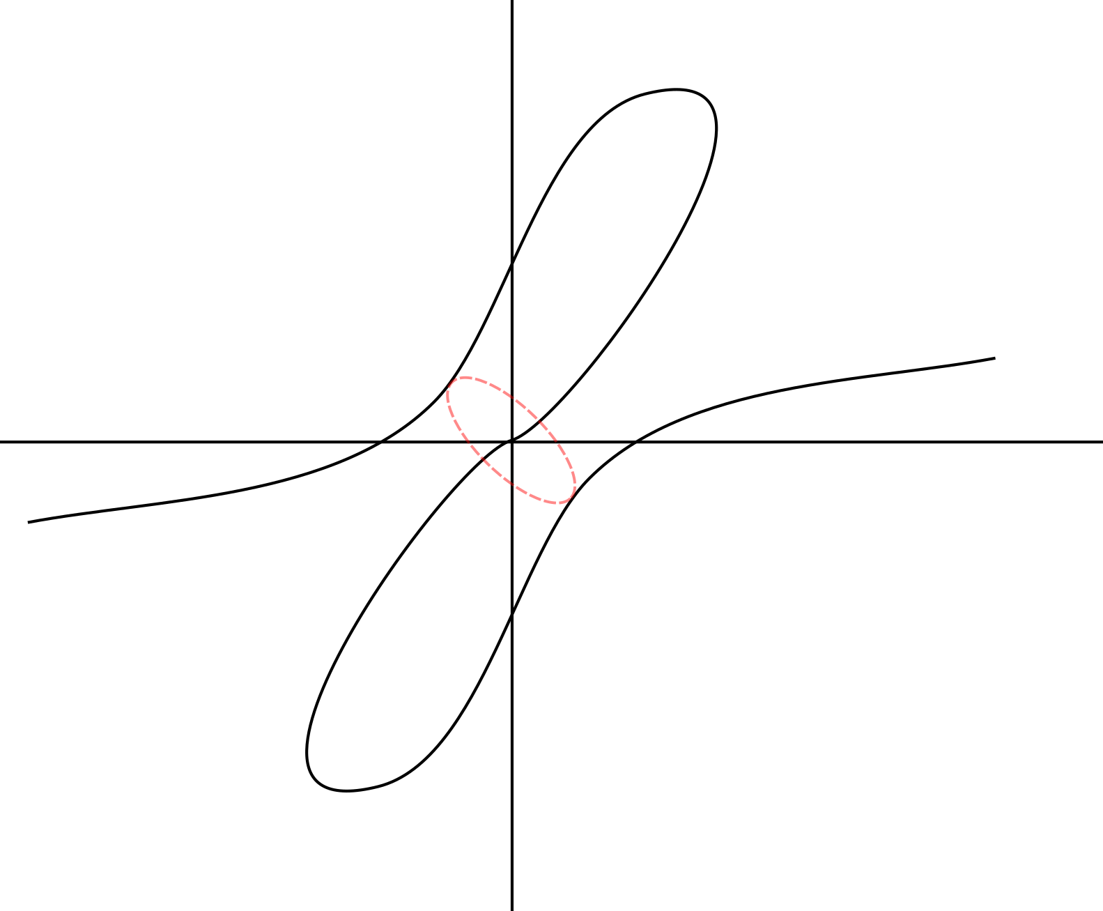
We consider two rational maps $\mathbb{CP}^{2}\to\mathbb{CP}^{1}$. The first is the Lefschetz fibration

$$f([x:y:z])=[xy:z^{2}]$$

in the complement of the anti-canonical divisor $D=\{(xy-z^{2})z=0\}$. The second is the projection

$$\pi([x:y:z])=[y:z].$$

This extends to a foliation of $\mathbb{CP}^{2}$ by holomorphic spheres each intersecting at a single point $[0:0:1]$ with intersection number 1.

We call a subset $U\subset\mathbb{C}$ point-symmetric if $x\in U$ if and only if $-x\in U$. For a point-symmetric curve $\gamma(s)\in\mathbb{C}$, define

$$L_{\gamma}^{0}=\left\{\left[\gamma(s)e^{i\alpha}:\gamma(s)e^{-i\alpha}:1\right]\,\big|\;\alpha\in\mathbb{R},s\in\mathbb{R}\right\}$$

and notice that since $\gamma$ is point-symmetric, $f(L_{\gamma}^{0})=\{[\gamma(s)^{2}:1]:s\in\mathbb{R}\}$ is an embedded curve in $\mathbb{CP}^{1}$ if $\gamma(s)$ is embedded in $\mathbb{C}$. We will also allow unions of two smooth non-intersecting curves such that the union is point-symmetric. By an abuse of notation, we refer to such a curve as $\gamma(s)$ where the parameter $s$ is now allowed to vary over two intervals or circles.

First, we identify various Lagrangians in this format. Let $\gamma(s)=s\in\mathbb{R}\subset\mathbb{C}$. Then

$$\{[se^{i\alpha}:se^{-i\alpha}:1]\}$$

lies above $\gamma$ and is compactified by the circle $[e^{i\alpha}:e^{-i\alpha}:0]$ at infinity. The resulting manifold is

$$L_{\mathbb{R}}^{0}:=\{[se^{i\alpha}:se^{-i\alpha}:1]\}\cup\{[e^{i\alpha}:e^{-i\alpha}:0]\}=\{[1:e^{-2i\alpha}:re^{-i\alpha}]\}\cup\{[0:0:1]\}$$

or equivalently, using the substitution $s=\cot\phi$,

$$L_{\mathbb{R}}^{0}=\{[\cos\phi e^{i\alpha}:\cos\phi e^{-i\alpha}:\sin\phi]:\phi\in[0,\pi/2],\alpha\in\mathbb{R}\}.$$

Note that $L_{\mathbb{R}}^{0}$ is fixed under the anti-symplectic involution $X:[x:y:z]\mapsto[\bar{y}:\bar{x}:\bar{z}]$, hence is isomorphic to $\mathbb{RP}^{2}$. The same applies for any other line through the origin in $\mathbb{C}$.

The curve $\gamma_{r}(s)=re^{is}$ lifts to a Lagrangian torus of Clifford-type, which is monotone and minimal if and only if $r=1$. Furthermore, any point-symmetric closed curve enclosing the origin lifts to a torus of Clifford-type, monotone if and only if the symplectic area contained is equal to $4\pi/6=2\pi/3.$ This follows from the Cieliebak–Goldstein formula (2.5), $\kappa=6$ and the fact that the disc is Maslov 4. Any closed circle $\gamma$ not enclosing the origin and its point-symmetric image $-\gamma$ together lift to a torus of Chekanov-type (provided $\gamma$ does not intersect $-\gamma$), monotone if and only if the area contained is $2\pi/6=\pi/3$. The fact that these Lagrangians are Clifford and Chekanov respectively can be checked by observing their images under the Lefschetz fibration $f$ and comparing with the standard definitions in Auroux, for instance, [4].

We will distinguish between Clifford tori and Chekanov tori by their intersections with real projective planes $\mathbb{RP}^{2}$. Immediately we observe that any closed curve $\gamma$ enclosing the origin intersects any line $l$ through the origin in at least two points, hence any equivariant Clifford torus $L_{\gamma}\cong L_{\text{Cl}}$ intersects $L_{l}\cong\mathbb{RP}^{2}$ in at least one circle. Indeed, this result is generalisable: $L_{\text{Cl}}$ is non-displaceable from $\mathbb{RP}^{2}$, as can be shown in multiple different ways (see for instance [5] or [10]). Indeed, Amorim and Alston [2] give a lower bound of 2 for the number of intersections between a Clifford torus and $\mathbb{RP}^{2}$. On the other hand, one can easily observe that there exists a pair of point-symmetric circles $\gamma(s)\in\mathbb{C}$ each containing a disc of area 2 and not intersecting the imaginary axis $i\mathbb{R}\in\mathbb{C}$. Hence Chekanov tori are displaceable from $\mathbb{RP}^{2}$.

In the sequel, it will be useful to consider cones of real projective planes intersecting our flowing Lagrangian tori, so we make the following definition:

Finally, we define the symmetry condition we will be using.

The point-symmetry is an $S^{1}$-symmetry on the level of $L_{\gamma}$, so the equivariance considered is an $(S^{1}\times\mathbb{Z}_{2})$-symmetry. The main reason for this symmetry condition is to greatly restrict the variety of singularities that can occur. Specifically, we want to have only Lawlor neck singularities occurring at the origin, with type I blow-up given by $C^{0}_{\pi/2}$. We shall see how the equivariance gives this in Section 5.2.

Before proceeding to the proofs of the main theorems, we calculate the evolution equation satisfied by the profile curve $\gamma$ under mean curvature flow. Despite being the governing equation for the rest of the results in the paper, we do not need the precise formulation frequently: it is only necessary for the explicit construction of various barriers. However, the derivation of the evolution equation for $\gamma$ is interesting in its own right since we calculate the mean curvature of $L_{\gamma}$ by a novel method.

Recall the fibration $\{L_{\alpha}\}$ by Clifford-type tori given by the fibres of the moment map

$$\mu([x:y:z])=\frac{1}{|x|^{2}+|y|^{2}+|z|^{2}}\left(|x|^{2},|y|^{2}\right).$$

The equivariant fibres are

$$L_{r}=\{L_{re^{i\phi}}:r>0\}$$

and for the rest of this paper, we denote by $\Omega$ the holomorphic volume form relative to $\{L_{\alpha}\}$. We first calculate the mean curvature of $L_{r}$, then we calculate the mean curvature of any other equivariant torus $L_{\gamma}$ by calculating the relative Lagrangian angle between $L_{\gamma}$ and $L_{r}$ using Theorem 2.3. Recall that Theorem 2.3 implies that the relative Lagrangian angle $\theta=\theta_{\operatorname{rel}}$ defined by $\Omega$ satisfies

$$H_{L_{\gamma}}(X)=d\theta_{\operatorname{rel}}(X)+H_{L_{r}}(\pi X)$$

where $\pi$ is the projection onto the tangent bundle of $L_{r}$.

We calculate the mean curvature 1-form of Clifford tori $L_{r}$ indirectly. The curve $\gamma(s)=re^{is}$ bounds a $J$-holomorphic disc which lifts to $\mathbb{CP}^{2}$ giving a disc

$$u:z\mapsto[rz:rz:1]$$

with boundary on $L_{r}$ of Maslov index 4. Cieliebak–Goldstein gives

$$-\int_{\partial D}H_{L_{r}}=6\int_{D}\omega-4\pi$$

since $\kappa=6$ for $\mathbb{CP}^{2}$ with the Fubini–Study metric. We calculate $\int_{D}\omega$ directly. We have that in radial coordinates $x=r_{1}e^{i\theta_{1}}$, $y=r_{2}e^{i\theta_{2}}$, the Kähler form is

	$\displaystyle\omega=\frac{1}{\left(1+r_{1}^{2}+r_{2}^{2}\right)^{2}}\Big($	$\displaystyle r_{1}(1+r_{2}^{2})dr_{1}\wedge d\theta_{1}-r_{1}r_{2}^{2}dr_{1}\wedge d\theta_{2}$
		$\displaystyle-r_{1}^{2}r_{2}dr_{2}\wedge d\theta_{1}+r_{2}(1+r_{1}^{2})dr_{2}\wedge d\theta_{2}\Big),$

so

(4.1)

$$\int_{D}\omega=2\pi\int_{0}^{r}\frac{2\tilde{r}}{(1+2\tilde{r}^{2})^{2}}\,d\tilde{r}=\pi\frac{2r^{2}}{1+2r^{2}}.$$

Hence using Cieliebak–Goldstein, we have

$$-\int_{\partial D}H_{L_{r}}=6\pi\frac{2r^{2}}{1+2r^{2}}-4\pi=4\pi\left(\frac{r^{2}-1}{1+2r^{2}}\right).$$

Note that $r=1$ is the monotone flat Clifford torus. Then by the symmetry of the tori $L_{r}$, we have that

(4.2)

$$H_{L_{r}}=-2\left(\frac{r^{2}-1}{1+2r^{2}}\right)ds$$

as a 1-form on $L_{r}$.

Next we calculate the relative Lagrangian angle. If $\gamma(s)=r(s)e^{i\phi(s)}$, then $L_{\gamma}$ is given by the embedding

$$F_{\gamma}:(s,\alpha)\to\left[r(s)e^{i\phi(s)}e^{i\alpha}:r(s)e^{i\phi(s)}e^{-i\alpha}:1\right].$$

Identifying the tangent space of $\mathbb{CP}^{2}$ in the coordinate patch where $z=1$ with $\mathbb{C}^{2}$ in the obvious way, we find that

$$\omega\left(\frac{\partial F_{\gamma}}{\partial s},\frac{\partial F_{\gamma}}{\partial\alpha}\right)=\omega\left(\partial_{r_{1}}+\partial_{r_{2}},\partial_{\theta_{1}}-\partial_{\theta_{2}}\right)=0,$$

which verifies that $L_{\gamma}$ is Lagrangian, and furthermore, we have

$$\Omega_{L_{r}}\left(\frac{\partial F_{\gamma}}{\partial s},\frac{\partial F_{\gamma}}{\partial\alpha}\right)=\Omega_{L_{r}}\left(-r^{-1}r^{\prime}J\partial_{\phi}+\phi^{\prime}\partial_{\phi},\frac{\partial F_{\gamma}}{\partial\alpha}\right),$$

where $\partial_{\phi}=\partial_{\theta_{1}}+\partial_{\theta_{2}}$ and we have used $J\partial_{\theta_{i}}=-r_{i}\partial_{r_{i}}$. Since $\frac{\partial F_{\gamma}}{\partial\alpha}$ is tangent to $L_{r}$, the Lagrangian angle $\theta$ relative to $\Omega_{L_{r}}$ is given by

$$\theta=\arg\left(\phi^{\prime}-ir^{\prime}r^{-1}\right)=-\tan^{-1}\left(\frac{r^{\prime}}{r\phi^{\prime}}\right)$$

and hence

(4.3)

$$d\theta=\frac{-r^{\prime\prime}r\phi^{\prime}+r^{\prime 2}\phi^{\prime}+r^{\prime}r\phi^{\prime\prime}}{r^{\prime 2}+r^{2}\phi^{\prime 2}}ds.$$

But the Euclidean planar curvature $k$ of $\gamma$ is

(4.4)

$$\begin{split}k&=\frac{-r^{\prime\prime}r\phi^{\prime}+2r^{\prime 2}\phi^{\prime}+r^{\prime}r\phi^{\prime\prime}+r^{2}\phi^{\prime 3}}{\left(r^{\prime 2}+r^{2}\phi^{\prime 2}\right)^{3/2}}\\ &=\left(\frac{-r^{\prime\prime}r\phi^{\prime}+r^{\prime 2}\phi^{\prime}+r^{\prime}r\phi^{\prime\prime}}{\left(r^{\prime 2}+r^{2}\phi^{\prime 2}\right)}+\phi^{\prime}\right)\frac{1}{\sqrt{r^{\prime 2}+r^{2}\phi^{\prime 2}}}\end{split}$$

We have that the projection of $\frac{\partial F_{\gamma}}{\partial s}$ onto $L_{r}$ is

$$\pi\left(\frac{\partial F_{\gamma}}{\partial s}\right)=\frac{\omega\left(\frac{\partial F_{\gamma}}{\partial s},J\frac{\partial F_{r}}{\partial s}\right)}{\omega\left(\frac{\partial F_{r}}{\partial s},J\frac{\partial F_{r}}{\partial s}\right)}\frac{\partial F_{r}}{\partial s}=\phi^{\prime}\frac{\partial F_{r}}{\partial s}$$

so we are led to conclude that

(4.5)

$$H_{L_{r}}\left(\pi\left(\frac{\partial F_{\gamma}}{\partial s}\right)\right)=-2\left(\frac{r^{2}-1}{1+2r^{2}}\right)\phi^{\prime}.$$

Combining the above equations, we obtain

	$\displaystyle H_{L_{\gamma}}=d\theta+H_{L_{r}}(\pi(\cdot))$	$\displaystyle=\left(k\sqrt{r^{\prime 2}+r^{2}\phi^{\prime 2}}-\phi^{\prime}-2\left(\frac{r^{2}-1}{1+2r^{2}}\right)\phi^{\prime}\right)\,ds$
		$\displaystyle=\left(k\sqrt{r^{\prime 2}+r^{2}\phi^{\prime 2}}+\left(\frac{1-4r^{2}}{1+2r^{2}}\right)\phi^{\prime}\right)\,ds.$

Hence we have that

$$\omega\left(\frac{\partial F_{\gamma}}{\partial s},\vec{H}_{L_{\gamma}}\right)=k\sqrt{r^{\prime 2}+r^{2}\phi^{\prime 2}}+\left(\frac{1-4r^{2}}{1+2r^{2}}\right)\phi^{\prime},$$

but

	$\displaystyle\omega\left(\frac{\partial F_{\gamma}}{\partial s},J\frac{\partial F_{\gamma}}{\partial s}\right)$	$\displaystyle=\omega\left(r^{\prime}(\partial_{r_{1}}+\partial_{r_{2}})+\phi^{\prime}(\partial_{\theta_{1}}+\partial_{\theta_{2}}),r^{\prime}r^{-1}(\partial_{\theta_{1}}+\partial_{\theta_{2}})-r\phi^{\prime}(\partial_{r_{1}}+\partial_{r_{2}})\right)$
		$\displaystyle=\left(r^{\prime 2}r^{-1}+r\phi^{\prime 2}\right)\omega\left(\partial_{r_{1}}+\partial_{r_{2}},\partial_{\theta_{1}}+\partial_{\theta_{2}}\right)$
		$\displaystyle=2\frac{r^{\prime 2}+r^{2}\phi^{\prime 2}}{(1+2r^{2})^{2}}.$

So we conclude that

$$\vec{H}_{L_{\gamma}}=\frac{1}{2}\left(1+2r^{2}\right)^{2}\left(k+\left(\frac{1-4r^{2}}{1+2r^{2}}\right)\frac{\phi^{\prime}}{\sqrt{r^{\prime 2}+r^{2}\phi^{\prime 2}}}\right)DF_{\gamma}(\nu)$$

where $\nu$ is the Euclidean normal to $\gamma$ in $\mathbb{C}$. Since $\langle\gamma,\nu\rangle=-r^{2}\phi^{\prime}/|\gamma^{\prime}|$, we have that the mean curvature flow of $F_{\gamma}$ in $\mathbb{CP}^{2}$ induces an equivariant flow on $\gamma$ given by

(4.6)

$$\frac{\partial\gamma}{\partial t}=\frac{1}{2}\left(1+2r^{2}\right)^{2}\left(k-\left(\frac{1-4r^{2}}{1+2r^{2}}\right)\frac{\langle\gamma,\nu\rangle}{r^{2}}\right)\nu$$

References

- [1] (1986) The normalized curve shortening flow and homothetic solutions. Journal of Differential Geometry 23 (2). Cited by: §1.
- [2] (2011) Floer cohomology of torus fibers and real Lagrangians in Fano toric manifolds. International Mathematics Research Notices. Cited by: §4.1.
- [3] (1991) Parabolic equations for curves on surfaces: part II. Intersections, blow-up and generalized solutions. The Annals of Mathematics 133 (1), pp. 171. Cited by: item 1.
- [4] (2007) Mirror symmetry and T-duality in the complement of an anticanonical divisor. Journal of Gökova Geometry Topology 1, pp. 51––91. Cited by: §2.1.1, §4.1.
- [5] (2009) Rigidity and uniruling for Lagrangian submanifolds. Geometry & Topology 13 (5), pp. 2881––2989. Cited by: §4.1.
- [6] (1978) The motion of a surface by its mean curvature. Princeton University Press. Cited by: Appendix A.
- [7] (2018) Evolution by mean curvature flow of Lagrangian spherical surfaces in complex Euclidean plane. Journal of Mathematical Analysis and Applications 462 (1), pp. 637––647. Cited by: §5.2.
- [8] (2010) A note on singular time of mean curvature flow. Mathematische Zeitschrift 266, pp. 921––931. Cited by: §2.2.
- [9] (2004) A note on mean curvature, Maslov class and symplectic area of Lagrangian immersions. Journal of Symplectic Geometry 2 (2), pp. 261––266. Cited by: §1, §2.5.
- [10] (2009) Rigid subsets of symplectic manifolds. Compositio Mathematica 145 (03), pp. 773––826. Cited by: §4.1.
- [11] (2020) Remarks on the self-shrinking Clifford torus. Journal für die reine und angewandte Mathematik (Crelle’s Journal) (765), pp. 139––170. Cited by: §2.1.1.
- [12] (2022) Lagrangian mean curvature flow in the complex projective plane. Ph.D. Thesis, University College London. Cited by: §2.5, §4.4, §4.4, §4.4, §4.4, item 3, §5.2, §5.2, §5.2, §5.2, Acknowledgments.
- [13] (1989) Shortening embedded curves. The Annals of Mathematics 129 (1), pp. 71. Cited by: §2.5.
- [14] (2007) Mean curvature flow of monotone Lagrangian submanifolds. Mathematische Zeitschrift 257 (2), pp. 295–327. Cited by: §3, §3.
- [15] (2009) Mean curvature flow with surgeries of two–convex hypersurfaces. Inventiones mathematicae 175 (1), pp. 137–221. External Links: ISSN 1432-1297, Link Cited by: §2.2.
- [16] (2015) Conjectures on Bridgeland stability for Fukaya categories of Calabi-–Yau manifolds, special Lagrangians, and Lagrangian mean curvature flow. EMS Surveys in Mathematical Sciences 2 (1), pp. 1––62. Cited by: §1, footnote 2.
- [17] (2018) From minimal Lagrangian to J-minimal submanifolds: persistence and uniqueness. Bollettino dell Unione Matematica Italiana. Cited by: §2.3.
- [18] (2013) Lecture notes on mean curvature flow. Springer Basel. Cited by: Appendix A.
- [19] (2007) Singularities of Lagrangian mean curvature flow: zero-Maslov class case. Inventiones mathematicae 168 (3), pp. 449––484. Cited by: Appendix A, §1, §4.1, §5.2.
- [20] (2010) Singularities of Lagrangian mean curvature flow: monotone case. Math. Res. Lett. 17 (1), pp. 109–126. External Links: ISSN 1073-2780, Link, Review MathReviews Cited by: Appendix A, §1, §5.2, §5.2, §5.2, §5.2.
- [21] (1994) Mean curvature vector and symplectic topology of Lagrangian submanifolds in Einstein-Kähler manifolds. Mathematische Zeitschrift 216 (1), pp. 471––482. Cited by: §2.3, §2.4.
- [22] The entropy formula for the Ricci flow and its geometric applications. Note: arXiv:math/0211159 Cited by: §2.2.
- [23] (2010) Notes on monotone Lagrangian twist tori. Electronic Research Announcements in Mathematical Sciences 17, pp. 104––121. Cited by: §2.1.1, §2.1.
- [24] A canonical way to deform a Lagrangian submanifold. External Links: Link Cited by: §2.2.
- [25] (1999) Harnack inequality for the Lagrangian mean curvature flow. Calculus of Variations and Partial Differential Equations 8 (3), pp. 247–258. External Links: ISSN 1432-0835, Link Cited by: §2.4.
- [26] (1836) Sur une classe d’equations a differences partielles. J. Math. Pures Appl. 1, pp. 373––444. Cited by: item 1.
- [27] (2002) Special Lagrangians, stable bundles and mean curvature flow. Communications in Analysis and Geometry 10 (5), pp. 1075––1113. Cited by: §1, §2.3, §2.4.
- [28] (2014) On exotic Lagrangian tori in . Geometry & Topology 18 (4), pp. 2419––2476. Cited by: §1.
- [29] (2016) Infinitely many exotic monotone Lagrangian tori in . Journal of Topology 9 (2), pp. 535––551. Cited by: §1, §2.1.1.
- [30] (2001) Mean curvature flow of surfaces in Einstein four-manifolds. J. Differential Geom. 57 (2), pp. 301–338. External Links: Link Cited by: §1, §2.2, §3.
- [31] (2019) Singularities of equivariant Lagrangian mean curvature flow. Note: ArXiv preprint, arXiv:1910.06122 External Links: Link Cited by: Appendix A, §1, §1, §5.2.
- [32] (2020) Singularities of Lagrangian mean curvature flow. Ph.D. Thesis, University College London. Cited by: Appendix A, §1, §1, item 4, §5.2.