Acknowledgments
First and foremost, I am extremely grateful to my supervisor and mentor, Professor Naftali Tishby, who passed away recently. His invaluable advice, continuous support, and patience during my Ph.D. study were so important. His immense knowledge and plentiful experience have encouraged me in all the time of my academic research and daily life. He was a remarkable man who gave me so much, and I learned a lot from him. An incredible scholar and a lovely person.
I would also like to thank Prof. Haim Sompolinsky and Dr. Alex Alemi for their support and guidance during my study. I wish to thank also my collaborators, Zoe Piran and Dr. Amichai Painsky. It was a great privilege to work with them.
Finally, I cannot begin to express my gratitude to my wife and children. Without their tremendous understanding and encouragement in the past few years, it would be impossible for me to complete my study. There were always there to support me and encourage me to succeed.
Abstract
While deep neural networks have been immensely successful, a comprehensive theoretical understanding of how they work or how they are structured does not exist. Deep networks are often viewed as black boxes, where the interpretation of predictions and their reliability are still unclear. Today, understanding the groundbreaking performance of deep neural networks is one of the greatest challenges facing the scientific community. To use these algorithms more effectively and improve them, we need to understand their dynamic behavior and their ability to learn new representations.
This thesis addresses these issues by applying principles and techniques from information theory to deep learning models to increase our theoretical understanding and use it to design better algorithms. The main results and contributions of this thesis are structured in three parts, as detailed below.
Chapters 2 and 3 present our information-theoretic approach to deep learning models. As an explanation for deep learning systems, we propose using the Information Bottleneck (IB) theory. The novel paradigm for analyzing networks sheds light on their layered structure, generalization capabilities, and learning dynamics. Based on our analysis, we find that deep networks optimize each layer’s mutual information on input and output variables, resulting in a trade-off between compression and prediction for each layer. Our analytical and numerical study of these networks demonstrated that the stochastic gradient descent (SGD) algorithm follows the IB trade-off principle by working in two phases: a fast empirical error minimization phase followed by a slow representation compression phase. These phases are distinguished by different signal-to-noise ratios (SNRs) for each layer. Moreover, we demonstrated that the SGD achieved this optimal bound due to the compression phase, derived a new Gaussian bound on the representation compression, and related it to the compression time. Furthermore, our results indicate that the network’s layers converge to the IB theoretical bound, leading to a self-consistent relationship between the encoder and decoder distributions.
Chapter 4 deals with one of the most difficult problems of applying the IB to deep neural networks — estimating mutual information in high dimnesional space. Despite being an important quantity in data science, mutual information has historically posed a computational challenge. Computing mutual information is only tractable for discrete variables or for a limited number of problems where probability distributions are known. To better estimate information-theoretic quantities and to investigate generalization signals, we research several frameworks and utilize recent theoretical developments, such as the neural tangent kernel (NTK) framework. In our study, we found that for infinite ensembles of infinitely wide neural networks, we could obtain tractable computations of many information-theoretic quantities and their bounds. Many quantities can be described in a closed-form solution by the network’s kernels. By analyzing these derivations, we can learn the important information-theoretic quantities of the network and how compression, generalization, and the sample size are related.
Chapter 5 presents the dual Information Bottleneck (dualIB), a new information-theoretic framework. Despite the IB framework’s advantages, it also has several drawbacks: The IB is completely non-parametric and operates only on the probability space. In addition, the IB formulation does not relate to the task of prediction over unseen patterns and assumes full access to the joint probability. Therefore, we developed the dualIB, which resolves some of the IB’s drawbacks through a mere switch between terms in the distortion function. The dualIB can account for known features of the data and use them to make better predictions over unseen examples. We provide dualIB self-consistent equations, allowing us to obtain analytical solutions. A local stability analysis revealed the underlying structure of the critical points of the solutions, resulting in a full bifurcation diagram of the optimal pattern representations. We discovered several interesting properties of dualIB’s objective. First, the dualIB retains its structure when expressed in a parametric form. It also optimizes the mean prediction error exponent, thereby improving prediction accuracy with respect to sample size. In addition to dualIB’s analytic solutions, we provided a variational dualIB framework that optimizes the functional using deep neural networks. The framework enables a practical implementation of dualIB for real-world datasets. With it, we empirically evaluated its dynamics and validated the theoretical predictions in modern deep neural networks.
In conclusion, this thesis proposes a new information-theoretic perspective for studying deep neural networks that draws upon the correspondence between deep learning and the IB framework. Our unique perspective can provide a number of benefits, such as attaining a deeper understanding of deep neural networks, explaining their behavior, and improving their performance. At the same time, our study opens up new theoretical and practical research questions.
Letter of Contribution
This dissertation includes four manuscripts that summarize Ravid Shwartz-Ziv’s research under the supervision of Naftali Tishby. The work on this dissertation was also done in collaboration with Dr. Alex Alemi (Google), Dr. Amichai Painsky (Tel Aviv University) and Zoe Piran (The Hebrew University). They provided valuable guidance and contributed to the writing of the papers as co-authors. The lead author and primary contributor for three of these manuscripts is Ravid Shwartz-Ziv. Ravid Shwartz-Ziv and Zoe Piran each contributed equally to the manuscript “The Dual Information Bottleneck.” For this manuscript, Ravid Shwartz-Ziv did the variational dual IB section and the numerical experiments. The manuscripts are listed below. One was published in a peer-reviewed venue, and three are yet to be published.
- 1.
“Opening the Black Box of Deep Neural Networks via Information”.
Co-author: Naftali Tishby. 2018. - 2.
“Representation Compression and Generalization in Deep Neural Networks”.
Co-authors: Amichai Painsky and Naftali Tishby. 2019. - 3.
“Information in Infinite Ensembles of Infinitely-Wide Neural Network”.
Co-author: Alex Alemi. Published in the Proceedings of the Symposium on Advances in Approximate Bayesian Inference, PMLR, 2020. - 4.
“The Dual Information Bottleneck”.
Co-authors: Zoe Piran and Naftali Tishby. 2020.
Table of Contents
Introduction
Learning representations is at the core of many problems in computer vision, natural language processing, cognitive science, and machine learning (bengio2013representation). A complex data representation is required for classification and prediction since physical parameters, such as location, size, orientation, and intensity, are considered (salakhutdinov2013learning). However, it is unclear what constitutes a good representation and how it is related to learning and to the specific problem type.
By combining multiple transformations of simple neurons, deep neural networks (DNNs) can produce a more useful (and, in most cases, more abstract) representation. Due to their versatility and success across various domains, these systems have gained popularity over the past few years. The performance of DNNs demonstrates great improvements over conventional machine learning methods in various domains, including images, audio, and text (devlin2018bert; he2016deep; oord2016wavenet). The latest deep learning models are more complex, and their architectures are becoming more complex with more parameters that need to be optimized. The ResNet- network, for example, contains about million parameters optimized over millions of images.
However, the reasons for these performances are only partially understood from a theoretical perspective, and we only have a heuristic understanding of them. It is unclear why deep models perform so well on real-world data and what their key components are. In addition, current metrics do not provide insight into the internal structure of a network or the quality of its layers. As a result, even if the model is extremely accurate, it is difficult to use it as a basis for further scientific research. To make these algorithms more effective and improve them, we must understand their underlying dynamic behavior and how they learn representations.
In this thesis, we propose studying DNNs from the perspective of information theory. As an explanation for modern deep learning systems, we propose the information bottleneck (IB) theory. We hope to shed light on their layered structures, generalization capabilities, and learning dynamics through this innovative approach for analyzing DNNs.
To better understand DNNs, the first question is as follows: How can information theory in general and the IB framework, in particular, be used to better understand DNNs?
Shannon invented the information theory to determine the number of bits needed to transmit a message over a noisy channel. This theory has since been shown to be an invaluable measure of the influence between variables (shannon1948mathematical). Given two random variables and , the mutual information between them measures the divergence of their joint probability distribution from the product of their marginals to determine how dependent or independent they are. The notion of mutual information, unlike correlation, can capture nonlinear statistical relationships between variables, strengthening our ability to analyze complex system dynamics (kinney2014equitability). Although mutual information is an essential quantity in data science, it has historically been challenging to estimate (paninski2003estimation). Exact computations are tractable only for a limited number of problems with well-defined probability distributions (e.g., the exponential family). The calculation of mutual information is not possible for finite samples of data or general problems.
This leads us to the following research question: How can we calculate the mutual information for large-scale DNNs? To derive an exact calculation of information-theoretic quantities and to search for generalization signals, we examined several frameworks and utilized current theoretical developments, including the Neural Tangent Kernel (NTK) framework (lee2019wide). We obtained tractable calculations of information-theoretic quantities and their bounds for infinite ensembles of infinitely-wide neural networks. Our analysis revealed that the kernels described many quantities in a closed form. Furthermore, we found that the input’s compression contributed to the generalization in this model family.
Although the IB framework has its advantages, it also has a few disadvantages, including an inability to preserve the structure of the data and suboptimal performance with finite data. The final research question concerns whether we can derive a new framework that can solve these problems and apply it to DNNs.
Therefore, we developed the dual IB (dualIB), which switches between the terms in the distortion function to solve some of the problems with the IB. A local stability analysis revealed the underlying structure and optimal pattern representations. We discovered that the dualIB retains its structure when expressed in a parametric form. Furthermore, it optimizes the mean prediction error exponent, improving the predictions’ accuracy with respect to sample size. dualIB can be applied to real-world datasets using neural networks with the help of a variational framework. Using this framework, we evaluated the dynamics of the dualIB and validated the theoretical predictions.
First, we examine some of the information-theoretic principles upon which this thesis is based. The chapter concludes by highlighting the main contributions of the thesis.
1.1 Information theory
In 1948, Shannon’s paper established the area of information theory (shannon1948mathematical). Communication, which refers to sending information with the receiver’s intent, is one of the main topics in information theory. Shannon’s work served as the basis for quantifying the questions regarding this information. Let us review the results of information theory relevant to this thesis. In the present work, we use the following notation: Upper-case letters denote random variables (e.g., ), calligraphic letters denote their support (e.g., ), and lower-case letters denote specific realizations (e.g., ).
1.1.1 Theoretical information quantities
As a formal concept, information is a function of several basic measures based solely on the probability distribution of random variables without any particular assumptions.
Consider and as random variables with the joint distribution function of . Our first definition of information is entropy, which takes into account the amount of uncertainty involved with a given distribution.
Definition 1.1.1.
Entropy
The entropy of is defined as
Shannon axiomatically derived this definition by defining three intuitive properties of uncertainty measures (continuity, additivity, and monotonicity). Entropy is the only function that satisfies these requirements. Intuitively, entropy reflects the minimum description length of because it is (roughly) the minimal number of bits or binary questions needed to determine the exact value of .
If the distribution is uniform, then the entropy reaches its maximum. If it is deterministic, then it is zero. As is concave, the more strays away from being completely unpredictable, the more it is punished by .
Our next informational measure is the Kullback-Leibler (KL) divergence, also known as relative entropy, which measures the divergence between two distributions.
Definition 1.1.2.
Kullback Leibler Divergence
The KL divergence between two distributions and is defined as
In the case where for some , then it will not contribute to . If for all , , then . When and have a low Kullback-Leibler distance, they are similar. Conversely, a high distance indicates they are dissimilar.
It can be shown that and that equality holds if and only if almost everywhere. Note that the KL divergence is not a metric because it is not symmetric and does not obey the triangle inequality. However, it is still useful to think of it as the natural ”distance” between distributions for several reasons. First, notice that is the expected log-likelihood ratio between and . Thus, it controls the discriminability between these two distributions when is the true underlying distribution of . Secondly, the KL divergence reflects the difference between the minimal description length of and the description length if is used instead of . To see this, notice that , and recall that is the minimal description length. Third, Pinsker’s inequality implies that the KL divergence upper bounds the distance between and . Therefore, it also bounds any distance for .
The last piece of information we will present is mutual information.
Definition 1.1.3.
Mutual Information
Let , and let and be their marginal distributions, respectively. The mutual information between and is defined as
Mutual information is a useful method for measuring statistical dependence between variables and has many beneficial properties. For example, it remains invariant under bijective transformations. Its predecessor, called the transmission rate, was first introduced by Shannon in 1948 (shannon1948mathematical) for a communication system. Mutual information can be axiomatically derived as a function satisfying several natural ‘informativeness’ conditions (cover1999elements).
Mutual information could be understood by thinking of the divergence between and the hypothetical joint distribution if and were independent.
It thus follows that and if and only if and are independent. Alternatively, mutual information can be interpreted as reducing uncertainty regarding one variable due to the knowledge of the other variable.
Since , it holds that . If , that is, is completely known given , then . As a special case, it holds that . In this sense, mutual information is more general than entropy, whereas entropy is sometimes referred to as self-information.
One of the important properties of mutual information is the data processing inequality (DPI), which implies that the information about contained in cannot be increased by processing . Formally, we say that form a Markov chain if their joint distribution can be decomposed as , is a function of and given , it is independent of . Then, the DPI implies
| (1.1) |
for any 3 variables that form a Markov chain .
Mutual information is also invariant with respect to invertible transformations:
| (1.2) |
for any invertible functions and .
1.2 Representation learning
Machine learning is a field of Artificial Intelligence (AI) that automatically learns and improves from experience. These models use an internal representation of the input based on prior observations or data records to make better decisions. Learning representations lie at the core of many computer vision problems, natural language processing, cognitive science, and machine learning (bengio2013representation). Even so, the question of what constitutes a good representation or the relationship between representation, learning process, and specific features of a problem remains unanswered.
David Marr (marr2010vision) defined representation as a formal system for making explicit particular entities and types of information that an algorithm can use to process information. In this thesis, we focus on the second part – the idea that algorithms operate on representations. Representation learning refers to learning structures in the data. This learning makes it easier to extract useful information to classify and make predictions based on the data (Goodfellow-et-al-2016-Book). The question of what a good representation is has many answers. For probabilistic models, a good representation often captures the posterior distribution of the underlying explanatory factors for the observed input (natureDeepLeraning). In their AI-tasks, Bengio and LeCun (BengioAndLecunMIT) introduced the concept of complex but highly structured dependencies. In most cases, the tasks require transforming a high-dimensional input structure into a low-dimensional output or learning low-level representations. Accordingly, most of the input’s entropy is not relevant for the output, and it is difficult to extract the input’s relevant features (TishbyZ15).
1.2.1 Large deviation theory and the Sanov theorem
Statisticians, information theorists, and machine learning scientists share concepts for defining and extracting the optimal representation from observations. How would we characterize the optimal representation of the random input variable ? In general, we would like to have a representation that achieves high values for some reward function. In addition, we aim to learn efficiently these representations by using an empirical sample of the (unknown) joint distribution, which will enable us to generalize to unknown datasets.
As we will see in the following section, the large deviation theory can be used to illustrate the idea that constraining information with the representation will produce a representation that is more likely to generalize. This approach is derived from the type analysis and the Sanov theorem (cover1999elements). It is presented here for an independent and identically distributed (i.i.d.) process, although a Markov type analysis is also available (csiszar1987conditional).
With the large deviation theory, we can understand the probability of rare events, i.e., events with an exponentially small probability. Type analysis is applied to analyze the most likely samples from a given probability distribution following a constraint. Sanov’s theorem identifies the rate function for large deviations of the empirical measure of a sequence of i.i.d. random variables. The type definition and the Sanov Theorem for i.i.d. processes (cover1999elements) are presented here with an adaptation of the annotation to our needs.
Let be i.i.d. random variables with values in a finite set and with a distribution . Denote by the set of probabilities on . Let be the empirical distribution of :
The law of large numbers states that almost surely. To define a rare event, we fix that does not contain . We are interested in the behavior of probabilities of the form , as .
It is a trivial observation that each possible value must appear an integer number of times among the samples . This implies, however, that the empirical measure cannot take arbitrary values.
Definition 1.2.1.
Type of the sequence is the relative proportion of occurrences of each value. That is, where is the number of times occurs in the sequence t.
By definition, each type contains only information about how often each value shows up in the sample, discarding the order in which they appear. The importance of it is that large numbers of sequences are associated with each type, and each type is associated with a single reward value . It is always the case that , where we define as the set of types associated with sequences of samples with length .
Theorem 1.2.1.
Sanov Let be i.i.d. sequence from . Let be a set of types that is equal to the closure of its interior.
where .
For our needs, we define the set to be all the types (and the sequences that are associated with them) that achieve a reward above the desired threshold ; i.e., .
Sanov’s theorem gives us an important insight: the most likely sequence to be selected as a type that is the closest from the perspective to the distribution (denoted as ). This insight can be formalized as a trade-off, where on one side, we have the reward , and on the other, we have . The selected solution is governed by a parameter , which is the Lagrange multiplier coefficient. Given the nature of the types, they can be visualized and represented as points of a simplex whose axes are the probabilities of each symbol to appear. In this space, the two crucial points are the maximal reward point (a deterministic point at the edge of the simplex) and . The trade-off parameter defines a set of distributions that form a line between these points. These are known as geodesic lines. No two points along this line have the same , and therefore they do not have the same value.
1.2.2 Minimal sufficient statistic
An alternative definition of what constitutes a good representation is based on minimal sufficient statistics.
Definition 1.2.2.
Let . Let , where is a deterministic function. We call T a sufficient statistic of for if forms a Markov chain.
Therefore, a sufficient statistic captures all the information about that is available in . The following theorem states this property:
Theorem 1.2.2.
cover1999elements Let be a probabilistic function of . Then, is a sufficient statistic for if and only if (iff )
As we can see, the sufficiency definition includes the trivial identity statistic . Such statistics accomplish nothing since all they do is ”copy” rather than ”extract” important information. Therefore, it is necessary to prevent statistics from using observations in an inefficient manner.
To address this issue, the concept of minimal sufficient statistics was introduced:
Definition 1.2.3.
(Minimal sufficient statistic (MSS)) A sufficient statistic is minimal if for any other sufficient statistic , there exists a function such that almost surely (a.s.).
MMS are the simplest sufficient statistics and induce the coarsest sufficient partition on . MSS try to group the values of into as few partitions as possible without sacrificing any information. In addition, MSS can be shown to be the statistic with all the available information about while retaining as little information about as possible. Generally, sufficient statistics are restricted, in the sense that their dimension always depends on the sample size, unless the data comes from an exponential family distribution (koopman1936distributions).
1.2.3 The Information Bottleneck
Since exact minimal sufficient statistics only exist for special distributions, tishby2000information relaxed this optimization problem in two ways: (i) allowing the map to be stochastic, defined as an encoder , and (ii) allowing the map to capture only as much as possible of , but not necessarily all of it. They introduced the Information Bottleneck (IB) as a principled approach to extract relevant information from observed signals related to a target. For a random variable , this framework finds the best trade-off between the accuracy and the complexity related to another random variable with a joint distribution. The IB has been used in several fields, including neuroscience (buesing2010spiking; palmer2015predictive), slow feature analysis (turner2007maximum), speech recognition (hecht2009speaker) and deep learning (TishbyZ15; shwartz2017opening; alemi2016deep).
Let be an input random variable, a target variable, and their joint distribution. A representation is a stochastic function of defined by a mapping . This mapping can be viewed as transforming into a representation of in the space.
The triple forms a Markov chain in that order w.r.t. the joint probability measure and the mutual information terms and .
As part of the IB framework, we aim to find a representation that extracts as much information as possible about (high performance), while compressing maximally (keeping small). We could also interpret it as extracting only the relevant information that contains about .
The DPI implies , so the compressed representation cannot convey more information than the original signal. As a result, there is a tradeoff between compressed representation and the preservation of relevant information about . The construction of an efficient representation variable is characterized by its encoder and decoder distributions, and , respectively. The efficient representation of means minimizing the complexity of the representation while maximizing . Formally, the IB optimization involves minimizing the following objective function:
| (1.3) |
where is a parameter that controls the trade-off between the complexity of and the amount of relevant information it preserves. Intuitively, we pass the information that contains about through a “bottleneck” via the representation . It can be shown that
| (1.4) |
IB representations can be found using the IB method, a variant of the Blatu Arimoto algorithm (blaArimo). For any , the conditions for a stationary point of equation 1.3, can be expressed via the following self-consistent equations (tishby2000information):
| (1.5) |
where is a normalization term. If , , and take values in finite sets, and is known, then alternating iterations of 1.5 locally converge to a solution, for any initial .
If we denote and , the optimal information curve is defined as the optimal values of the trade-off for some . The information plane is the two-dimensional plane in which the IB curve resides. The equations in 1.5 are satisfied along the information curve, which separates the feasible and unfeasible regions of the information plane by a monotonic concave line.
1.3 Deep neural networks
In 1958, Frank Rosenblatt developed the perceptron algorithm, the first artificial neural network component (rosenblatt1958perceptron). The system was designed to mimic the way the human brain processes visual data and identifies recognizable objects. It was extended to pattern recognition in the late 1980s.
Deep learning can perform hierarchical learning of the data by applying nonlinear transformations, which distinguishes it from traditional neural networks. The data are cumulatively passed across multiple layers, which may be fully connected or partially connected. DNNs are multilayer structures constructed by processing units that are called neurons. Each neuron’s activation involves the weighted summation of neuron inputs from the previous layer, followed by the transfer function’s operation. Interconnected layers of these basic computing blocks are used to build complex deep learning architectures (DBLP:journals/corr/Schmidhuber14). Using this structure, DNNs can learn hierarchically sophisticated features directly from raw data without manually constructing them (salakhutdinov2013learning). Deep architectures are often more challenging to effectively train. They bring, however, two significant advantages: (1) they promote the reuse of features, and (2) they can potentially lead to progressively more abstract features at higher layers of representation, which hopefully make it easier to separate the explanatory factors in the data (erhan2009difficulty).
Although deep architectures have long existed, the term “deep learning” was first used in by hinton2006fast. This work showed that a multilayer feedforward neural network could be more efficient by applying pretraining of one layer at a time and considering each layer as an unsupervised Restricted Boltzmann Machine (RBM) by using supervised backpropagation for finetuning. In 2007, bengio2007greedy developed the Stack AutoEncoder (SAE), which comprises a deep architecture of many AutoeEcoders (AEs).
In 2012, krizhevsky2012imagenet proposed the AlexNet architecture, which won the ImageNet challenge. This was a significant breakthrough in artificial neural networks. They proposed a deep convolutional neural network with nine layers and implemented it over GPUs for the first time. Several extensions of the vanilla AlexNet network have been developed since then, including deeper convolutional nets as proposed by simonyan2014very and residual connections as demonstrated by ren2015faster. DNNs have demonstrated their ability to improve state-of-the-art results in a wide range of machine learning tasks over the past few years. In many areas, from visual object recognition to speech recognition and genomics to drug discovery, they work well and enhance state-of-the-art results dramatically (DBLP:journals/corr/abs-1303-5778; DBLP:journals/corr/ZhangL15; DBLP:journals/corr/abs-1207-0580; DBLP:journals/corr/HeZRS15; natureDeepLeraning).
1.4 Information Bottleneck and DNNs
Even though DNN has been highly successful, little is known about its reasons for success, and no underlying principles have driven its development. DNNs are often considered black boxes, where the interpretation of predictions and reliability are still open questions. Additionally, their internal structure and the optimization process are still not fully understood. To use these algorithms more efficiently and improve them, we need to understand their dynamic behavior and their ability to learn representations.
In the literature, two areas of work involve DNNs and the IB. One uses the IB concept to analyze DNNs, while the other uses the IB to improve the learning algorithm for DNNs. The rest of this section is divided into these categories.
1.4.1 Information Bottleneck as optimization objective
Recently, the IB framework was explored as an objective for deep learning. This concept was achieved by optimizing the IB Lagrangian using a variational bound (alemi2016deep; olchinsky2019nonlinear).
The variational information bottleneck (VIB) approach presented in (alemi2016deep) used DNNs to parameterize the IB model. A variational approximation of the objective is parametrized using DNN, and an efficient training algorithm is suggested for obtaining a stochastic network that maps inputs to randomized representations.
Given a DNN, denote its output representation as , a randomized mapping operating on the input feature , where the corresponding label is . The encoding of into is defined through a conditional probability distribution, which is parametrized as . The VIB optimization objective is
| (1.6) |
However, since the data distributions and are unknown, a direct optimization of Equation 1.6 is intractable. To overcome it, alemi2016deep suggested to lower bound Equation 1.6 in a form that we can optimize:
| (18) |
In this case, we parametrize the decoder by a DNN. However, the main difficulty of this optimization is intractable marginal distribution . To circumvent this, we take and distributions with a closed-form KL solution. In this case, we treat the network output’s encoder as the parameters of .
Using the reparametrization trick from kingma2013auto and replacing with its empirical proxy, the loss function of IB can be approximated as
| (19) |
is an auxiliary noise variable, and the expectation is w.r.t to its law. Note that if represents the output of a DNN, the first term is cross-entropy, which is derived from the loss function common in deep learning. The second term acts as a regularization term that penalizes the dependence of on , thus encouraging compression. An unbiased estimate of the true variational lower bound can be obtained through standard stochastic gradient-based methods by calculating the estimator’s gradient.
Since alemi2016deep, various extensions have been developed, demonstrating promising attributes (strouse2017deterministic; elad2019direct; kolchinsky2019nonlinear). Recently, the conditional entropy bottleneck (CEB) (fischer2020ceb) has been proposed. The CEB provides variational optimizing bounds on and using a variational decoder , variational conditional marginal, , and a variational encoder, , all implemented by DNNs. alemi2016deep also showed that the variational auto-encoder (VAE) (kingma2013auto) can be considered as an estimation for a special case of IB when , and the prior distribution function is fixed.
1.4.2 Information Bottleneck theory for deep learning
TishbyZ15 proposed a theoretical framework to analyze DNNs based on the principle of the IB. They formulated the ultimate goal of the network as a trade-off between compression and prediction. An optimal point on the information curve exists for each layer where this trade-off can be addressed effectively. The layer’s network structure forms a Markov chain, where each layer processes inputs from the previous layer. Due to DPI, any loss of information about in one layer is not recoverable in higher layers.
Formally, define as the compressed representation of in the i-th layer and as the network’s output. is uniquely mapped to a single point in the information-plane with coordinates . We map a network with layers to monotonic connected points in the plane. For any , it holds that
| (1.7) |
and the equality in the second line is achieved IFF each layer is a sufficient statistic of its input. Using this framework, each layer should extract a compact representation while preserving the relevant information.
By successively decreasing , we shift the network from low representations and construct higher and more abstract ones. On the one hand, measures how much of the predictive features in for is captured by the layer and can view it as an upper bound of the layer’s quality. On the other hand, can be interpreted as the complexity of the layer. As a result, we can assess the performance of DNNs not just in terms of output, as we do when we use other measures of error when evaluating DNNs.
Based on the theoretical IB limit and the limitations imposed by the DPI on the information flow between layers, we can get a good sense of each layer’s optimality in the network. With each successive layer, the IB distortion level increases, but it also compresses the inputs, hopefully removing only non-relevant information (TishbyZ15).
.9
1.4.3 Information bounds on the generalization gap
Based on the statistical learning theory, models with many parameters tend to overfit by modeling learned data too accurately, which reduces their ability to generalize to new data (boucheron2005theory). In practice, however, we see that DNNs have a minimal generalization gap between training and testing. Recently, there has been much interest in understanding implicit regularization. Researchers’ findings indicate that network size is not the most important factor involved in the process of learning multilayer feedforward networks and that some unknown factors are important (neyshabur2014search). Moreover, conventional statistical learning theories, such as Rademacher complexity, VC-dimension, and uniform stability (stavac; bartlett2002rademacher; bousquet2002stability), do not explain all of the unexpected results of numerical experiments. According to zhang2016understanding, regularization plays a unique role in deep learning that differs from empirical risk minimization. However, convincing experiments have indicated that the generalization gap can be reduced even without explicit regularization. In recent years, several works have demonstrated that the mutual information between the training inputs and the inferred parameters provides a concise bound on the generalization gap (xu2017information; pensia2018generalization; NIPS2019_9282; NIPS2018_7954; russo2016controlling; steinke2020reasoning; achille2019information). achille2018emergence investigated how using an IB objective on network parameters (rather than the representations) could avoid overfitting while enforcing invariant representations.
1.5 Infinitely-wide neural networks
Neural tangent kernel (NTK) is a powerful theoretical tool for modeling neural networks. lee2019wide showed that if neural network training is modeled as gradient flow, the training trajectory can be modeled by ordinary differential equations (ODEs). Equations like these represent a finite-width tangent kernel encoded by the network architecture and its current time-dependent weights. Moreover, they showed that if one scales the learning rate per layer appropriately (”NTK parametrization”) and lets the width tend to infinity, this kernel converges to the infinite-width NTK. By being independent of weights and staying constant throughout training, this model simplifies the ODE in this limit. They showed that for loss, the predictor at convergence would be produced by a kernel regression using an infinite-width NTK. Importantly, the NTK depends only on the architecture of the network and is not learned.
Infinitely-wide neural networks behave as they are linear in their parameters (lee2019wide):
| (1.8) |
This makes them particularly analytically tractable. An infinitely-wide neural network, trained by gradient flow to minimize the squared loss, admits a closed form expression for the evolution of its predictions as a function of time:
| (1.9) |
Here, denotes the output of our neural network acting on the input . is a dimensionless representation of the time of our training process. denotes the whole training set of examples, with their targets ; denotes the neural networks output at initialization. The evolution is governed by (the NTK). For a finite width network, the NTK corresponds to , the neural network gradients’ gram matrix. As the network’s width increases to infinity, this kernel converges in probability to a fixed value. Tractable ways to calculate the exact infinite-width kernel for broad classes of neural networks are available (lee2019wide). The shorthand denotes the kernel function evaluated on the train data ().
Observe that infinitely-wide networks trained with gradient flow and squared loss behave as affine transformations of their initial predictions. As a result, for an infinite ensemble of such networks, if the initial weight configurations are drawn from a Gaussian distribution, the law of large numbers guarantees the distribution of the output conditioned on the input is Gaussian. As the evolution is an affine transformation of the initial predictions, the predictions remain Gaussian throughout.
| (1.10) | ||||
| (1.11) | ||||
| (1.12) |
Here, denotes another kernel, the neural network gaussian process kernel (NNGP). For a finite width network, the NNGP corresponds to the expected gram matrix of the output- . In the infinite width limit, this concentrates to a fixed value. Just as for the NTK, the NNGP can be tractably computed (lee2019wide) and should be considered only a function of the neural network architecture. These results, which give us a conditional posterior distribution for each time step, enable us to create a powerful model family to investigate DNNs. These tractable distributions can be used to derive many intractable information-theoretic quantities.
1.6 The impact of the work
In summary, the IB theory offers a new perspective on DNNs and their capability to learn meaningful representations. This theory suggests studying the system by grouping each layer in the network into two information pairs, one with input and another with output: .
Following this study, which provided a theoretical foundation for understanding deep learning, several studies have offered further explorations of DNNs using information theory tools. We now discuss some of these works and whether they support or challenge our claims. A partial list includes achille2018emergence; saxe2019information; yu2020understanding; cheng2018evaluating; goldfeld2018estimating; wickstrom2019information; amjad2019learning; goldfeld2020convergence; cvitkovic2019minimal.
Following this study, several researchers have analyzed the information plane using different estimation mechanisms in various DNN datasets, architectures, and activation functions. They found conflicting results: The authors of saxe2019information did not observe compression in DNNs with ReLU activation functions. However, according to chelombiev2019adaptive, compression can occur earlier in training or later in training, depending on how the DNN parameters are initialized. goldfeld2018estimating developed a noisy DNNs framework with a rigorous estimator for . Using this estimator, they observed the input’s compression in various models. The authors related the noisy DNN to an information-theoretic communication problem, demonstrating that compression is driven by the progressive clustering of inputs belonging to the same class. The study clarified the geometric effects of mutual information compression during training. Other methods that have been proposed for estimating mutual information in DNNs are generative decoder networks (darlow2020information; nash2018inverting), the mutual information neural estimator (MINE) (elad2019direct), ensemble dependency graph estimator (EDGE) (noshad2018scalable), adaptive approaches for density estimation (chelombiev2019adaptive), and noisy sounding entropy estimator (goldfeld2018estimating), and more. For a detailed review of these works, see geiger2020information.
In another line of research, our idea was used to analyze networks using information with the weights (achille2018emergence; achille2018critical; achille2018information). It has been demonstrated that flat minima, which have better generalization properties, bound the information with the weights, which bounds the information with the activations. In achille2018critical, they used Fisher information on the weights to illustrate the two stages of learning that DNNs go through: increasing the information followed by progressively decreasing the information. By compressing the information with the weights, the network also compresses the information with the activations.
As shown in achille2018information, minimizing a stochastic network using an approximation of the compression term as a regularizer is equivalent to minimizing cross-entropy over deterministic DNNs with multiplicative noise (information dropout). In addition, they found that Bernoulli noise is a special case that leads to the dropout method. elad2019direct shows that the binned information can be interpreted as a weight decay penalty, which is typical of DNN training.
Furthermore, many competing information objectives have been proposed for training DNNs based on the IB principle, which can be difficult to compute for high dimensions. kirsch2020unpacking examined these quantities and compared, unified, and related them to surrogate objectives that are more easily optimized. The unifying view provided insights into IB training limitations and demonstrated how to avoid the pathological behavior of IB objectives. In addition, they discussed how simple objectives, based on this intuition, could capture many desirable features of IB algorithms while also scaling to complex deep learning problems. Furthermore, they explored how applying practical constraints to a neural network’s expressivity can provide new insights into measuring compression and possibly improving regularization.
1.7 Overview and main contributions
The purpose of our thesis is to provide an explanation of deep learning by using an information-theoretic framework, supported by empirical evidence, and overcoming some of the shortcomings of IB. We have outlined the major results and contributions of the thesis in three sections below:
- •
Part 1 – Opening the Black Box of Deep Neural Networks – The first contribution of this thesis is a presentation of an information-based theory for DNNs. Combining two papers shows that DNNs can learn to optimize the mutual information that each layer preserves on the input and output variables, resulting in a trade-off between compression and prediction. We present a theoretical and numerical analysis of DNNs in the information plane and explain how the SGD algorithm follows the information bottleneck trade-off principle. SGD achieves this optimal bound by compressing each layer to a maximum conditional entropy state subject to the constraints of the labels’ information. Moreover, we find that the network’s training is characterized by a rapid increase in the mutual information between the layers and the target label, followed by a slower decrease in the mutual information between the layers and the input variable. By introducing a new generalization error bound, which is exponential in the input representation compression, we propose a novel analytic bound on the mutual information between successive layers in the network. Combining these with the empirical case study enables a comprehensive understanding of optimization dynamics, SGD training properties, and deep architectures’ computational benefits.
- •
Part 2 – Information in Infinite Ensembles of Infinitely-wide neural networks – As previously mentioned, it is often challenging to measure information-theoretic quantities. We developed tractable computations for a wide range of information-theoretic quantities using the NTK framework. These results are used to investigate the critical quantities that correlate with generalization, dynamics, and optimality during the learning process in high-dimensional networks.
- •
Part 3 – The Dual Information Bottleneck – As mentioned before, the IB framework has several known drawbacks, including that it is not optimal for training with finite samples and that it does not preserve the problem structure. We present the dualIB, a framework for addressing some of these shortcomings. By switching the order between the representation decoder and data in the IB’s distortion function, the optimal decoding becomes the geometric mean of input points instead of the arithmetic mean. Whenever the data can be modeled in a parametric form, this conversion preserves its structure and, thus, the original properties of the data. Furthermore, the prediction accuracy is improved by optimizing the mean prediction error exponent for each data size. By analyzing the framework’s structure, we show how to solve this new representation learning formulation. A variational formulation of the dualIB for DNNs, (VdualIB) is presented to address large-scale problems. We examine its properties using real-world datasets and compare them to the original IB.
Opening the Black Box of Deep
Neural Networks via Information
Unpublished
Ravid Shwartz-Ziv and Naftali Tishby (2018)
Opening the Black Box of Deep Neural Networks via Information
Ravid Shwartz-Ziv 1 Naftali Tishby1,2
1 The Edmond and Lilly Safra Center for Brain Sciences, The Hebrew University,
Jerusalem, Israel.
2 School of Computer Science and Engineering,
The Hebrew University,
Jerusalem, Israel.
Abstract
Despite their great success, there is still no comprehensive theoretical understanding of learning with Deep Neural Networks (DNNs) or their inner organization. Previous work suggested analyzing DNNs in the Information-Plane; the plane of the mutual information values that each layer preserves on the input and output variables. They suggested that the network’s goal is to optimize the Information Bottleneck (IB) trade-off between compression and prediction, successively, for each layer. In this work, we demonstrate the effectiveness of the information-plane visualization of DNNs. We first show that the stochastic gradient descent (SGD) epochs have two distinct phases: fast empirical error minimization followed by slow representation compression for each layer. We then argue that the DNN layers end up very close to the IB theoretical bound and present a new argument for the hidden layers’ computational benefit.
Introduction
DNNs heralded a new era in predictive modeling and machine learning. Their ability to learn and generalize has set a new bar on performance, compared to state-of-the-art methods. This improvement is evident across almost every application domain (DBLP:journals/corr/abs-1303-5778; DBLP:journals/corr/ZhangL15; DBLP:journals/corr/abs-1207-0580; DBLP:journals/corr/HeZRS15; natureDeepLeraning).
However, despite their success, there is still little understanding of their internal organization or optimization process. They are often seen as mysterious ”black boxes” (probes2016).
The authors in TishbyZ15 pointed out that layered neural networks’ representations of input layers form a Markov chain. They suggested studying these in the information-plane - The plane of the mutual information values of any other variable with the input variable and the desired output variable (Figure 1.4). The rationale for this analysis was based on the mutual information’s invariance to invertible re-parameterization and the data processing inequalities (DPI) (Cover:2006) along the Markov chain of the layers. Moreover, they suggested that optimized DNNs layers should approach the Information Bottleneck (IB) bound (DBLP:journals/corr/Tishby1999) of the optimally achievable representations of the input .
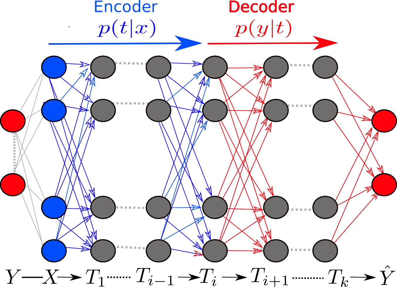
In this paper, we extend their work and demonstrate the effectiveness of visualizing DNNs in the information-plane to understand better the training dynamics, learning processes, and internal representations of deep learning.
Our analysis reveals that the SGD optimization, commonly used in deep networks, has two different and distinct phases: empirical error minimization (ERM) and representation compression. Each of these phases displays a very different signal-to-noise ratio of the stochastic gradients. During the ERM phase, gradient norms are much larger than their stochastic fluctuations, leading to a sharp increase in the mutual information on the label variable . At the compression phase, the errors fluctuate much more than their means, causing the weights to change much like Weiner processes, or random diffusion, with a small influence of error gradients. In this phase, the input variable undergoes slow representation compression or reduction of the mutual information.
In our experiments, most of the optimization iterations are spent on compressing the internal representations under the training error constraint. This compression occurs by the SGD without any other explicit regularization or sparsity imposed. We suspect that this helps avoid overfitting in deep networks. This observation also suggests that many (exponential in the number of weights) different randomized networks have essentially optimal performance. Hence, the interpretation of a single neuron (or weight) in the layers is practically meaningless.
Then we show that the optimized layers lay on or relatively close to the optimal IB bound for large enough training samples, resulting in a self-consistent relationship between each layer’s encoder and decoder distributions (Figure 1.4). The hidden layers in the optimized model converge along particular lines in the information-plane and move up as the training sample size increases. In addition to this, the diffusive nature of the SGD dynamics explains the computational benefit of the hidden layers.
Information Theory of Deep Learning
In supervised learning, we are interested in good representations, , of the input patterns , which enable good predictions of the label . Moreover, we want to efficiently learn such representations from an empirical sample of the (unknown) joint distribution , in a manner that provides good generalization.
DNNs generate a Markov chain of such representations, the hidden layers, by minimizing the empirical error over the network’s weights, layer by layer. This optimization occurs via SGD, using a noisy estimate of the empirical error gradient at each weight through the backpropagation algorithm (rumelhart1986learning).
Our first important insight is to treat the whole layer , as a single random variable, characterized by its encoder, , and decoder, distributions. As we are only interested in the information flowing through the network, invertible transformations of the representations that preserve information generate equivalent representations even if the individual neurons encode entirely different input features. For this reason, we quantify the representations by two numbers, or order parameters, that are invariant to any invertible re-parameterization of , the mutual information of with the input , , and the desired output , .
Next, the layers’ quality is quantified by comparing them to the information-theoretic optimal representation - the IB representations. Furthermore, we explore how the SGD can be used to obtain these optimal representations in DNNs.
Mutual information
Given any two random variables, and , with a joint distribution , their mutual information is defined as:
| (1.13) | ||||
| (1.14) | ||||
| (1.15) |
where is the Kullback-Liebler divergence of the distributions and , and and are the entropy and conditional entropy of and , respectively.
The mutual information quantifies the number of relevant bits that the input variable contains about the label , on average. The optimal learning problem can be cast as the construction of an optimal encoder of that relevant information via an efficient representation - a minimal sufficient statistic of with respect to . A minimal sufficient statistic can enable the decoding of the relevant information with the smallest number of binary questions (on average); i.e., an optimal code. The connection between mutual information and minimal sufficient statistics is discussed in the next section.
Among the characteristics of mutual information, two stand out particularly in relation to DNNs. The first is its invariance to invertible transformations:
| (1.16) |
for any invertible functions and .
The second is the DPI – (Cover:2006) For any three variables that form a Markov chain ,
The information-plane
Any representation variable, , defined as a (possibly stochastic) map of the input , is characterized by its joint distributions with and , or by its encoder and decoder distributions, and , respectively. Given , is uniquely mapped to a point in the information-plane with coordinates . When applied to the Markov chain of a K-layers DNN, with denoting the hidden layer as a single multivariate variable (Figure 1.4), the layers are mapped to monotonic connected points in the plane. Therefore, a unique information path which satisfies the following DPI chains:
Layers related by invertible re-parametrization appear at the same point, meaning that each information path in the plane corresponds to a multitude of different DNNs, possibly corresponding to very different architectures.
The Information Bottleneck optimal bound
What characterizes the optimal representations of w.r.t. ? The classical notion of minimal sufficient statistics provides good candidates for optimal representations. Sufficient statistics, in our context, are maps or partitions of , , capturing all the information that has on . Namely, (Cover:2006).
Minimal sufficient statistics, , are the simplest sufficient statistics and induce the coarsest sufficient partition on . Thus, they are functions of any other sufficient statistic. A simple way of formulating this is through the Markov chain: , which should hold for a minimal sufficient statistics with any other sufficient statistics . Using DPI, we can cast it into a constrained optimization problem:
Since exact minimal sufficient statistics only exist for special distributions (i.e., exponential families), DBLP:journals/corr/Tishby1999 relaxed this optimization problem by first allowing the map to be stochastic, defined as an encoder , and then, by enabling the map to capture as much as possible of , not necessarily all of it.
This leads to the IB trade off (DBLP:journals/corr/Tishby1999), which provides a computational framework for finding approximate minimal sufficient statistics, or the optimal trade-off between compression of and prediction of . In that sense, efficient representations are approximate minimal sufficient statistics.
If we define as the compressed representations of , the representation of is now defined by the mapping . This IB trade-off is formulated by the following optimization problem, carried independently for the distributions, , with the Markov chain: ,
| (1.17) |
The Lagrange multiplier determines the level of relevant information captured by the representation , , which is bounding the error in the label prediction from this representation. The local optimal solution to this problem is given by three self-consistent equations, the IB equations:
| (1.18) |
where is the normalization function. These equations must be satisfied along the information curve which is a monotonic concave line that separates the achievable and unachievable regions in the information-plane. For smooth distributions; i.e., when is not a completely deterministic function of , the information curve is strictly concave with a unique slope, , at every point, and a finite slope at the origin. In these cases, determines a single point on the information curve with specified encoder, , and decoder, , distributions that are related through Eq.(1.18).
Visualizing DNNs in the information-plane
As proposed by TishbyZ15, we study the information paths of DNNs in the information-plane. It is possible to do so when the underlying distribution, , is known and the encoder and decoder distributions, and , can be derived directly. In ”real-world” problems, these distributions and mutual information values should be estimated from samples or other modeling assumptions. We use two order parameters, and , to visualize and compare different network architectures in terms of their efficiency in preserving the relevant information in .
By visualizing the paths of different networks in the information-plane, we explore the following fundamental issues:
- 1.
The SGD layer’s dynamics in the information-plane.
- 2.
The effect of the training sample size on the layers.
- 3.
The benefit of the hidden layers.
- 4.
The final location in the information-plane of the hidden layers.
- 5.
The optimality of the layers’ representation.
Experiments
This section is organized as follows; First, we describe the experimental settings. Next, we discuss the results of our experiments, including the dynamics of the optimization process in the information-plane, the stochastic gradients, and the computational benefit of the hidden layers. In the last part, we present the layers’ optimality and their evolution with the training size.
Experimental setup
The numerical studies in this paper explore fully connected feed-forward neural networks with no further architecture constraints. The activation function of all hidden layers is the hyperbolic tangent function. For the final layer, we use a sigmoidal function. The networks train using SGD and the cross-entropy loss function (with no explicit regularization). Unless otherwise noted, the DNNs use up to seven fully connected hidden layers, with widths of neurons (see Figure ). In our results below, layer one is the hidden layer closest to the input and the highest is the output layer.
To simplify our analysis, the tasks were chosen as binary decision rules, which are invariant under rotations of the sphere. We define the input to be binary inputs representing uniformly distributed points on a sphere (for other, non-symmetric rules, see Supplementary material). The different patterns of the input variable are divided into disjoint orbits of the rotation group. These orbits form a minimal sufficient statistics for spherically symmetric rules (Kazhdan2003).
Given a function defined on the sphere, we can obtain a rotation and reflection invariant representation by computing the spherical harmonic decomposition of the function.
and calculate the energy ( norms) of the frequency components.
| (1.19) |
We refer the reader to Kazhdan2003 for a good exposition on the above. To generate the input-output distribution, , we consider spherically symmetric real valued function of the pattern minus a threshold, , and apply a sigmoidal function, :
| (1.20) |
The threshold was selected such that , with uniform . The sigmoidal gain was high enough to keep the mutual information bits.
Estimating the mutual information of the layers
As mentioned above, we model each layer in the network as a single variable , and calculate its mutual information with the input and the labels.
To calculate the mutual information of the networks’ layers with the input and output variables, we binned the neuron’s output activation into equal intervals between and . These discretized values for each neuron in the layer, , are used to directly calculate the joint distributions, over the equally likely input patterns , and , using the Markov chain for every hidden layer. Using the above discrete joint distributions, we calculate the decoder mutual information, , and the encoder mutual information, , for each hidden layer. Note that is calculate with the full data distribution; thus, it corresponds to the generalization error.
We repeat these calculations with different randomized initialization of the network’s weights and different random selections of the training samples, randomly distributed according to the rule in Eq.(1.20).
The dynamics of the optimization process
To understand the network’s SGD optimization dynamics, we evaluate and visualize pairs of and for each layer along the learning process. We repeat this process for different randomized initializations with different randomized training samples. Figure 1.6 depicts the layers (each one in a different color) of all the networks, trained with a randomized percents of the input patterns, in the information-plane, at various times during the training.
As can be seen, the deeper layers of the randomly-initialized network do not preserve the relevant information at the beginning of the optimization, and decreases sharply along the path. During the SGD optimization, the layers first increase , then significantly decrease – compressing the representation. One striking observation is that the different randomized networks’ layers follow similar paths through the optimization process and eventually converge to nearby points in the information-plane. The randomized networks are thus averaged over, and the average layer trajectory plot is shown in Figure 1.8.


The graph on the left shows those same trajectories when trained with percent of all patterns, whereas on the right, the same trajectories when trained with only percent. Note that the mutual information is calculated with the full rule distribution. Thus, corresponds to the test or generalization error. In each case, the two optimization phases are visible. During the fast - ERM phase, which lasts a few hundred epochs, the layers increase the information on the labels (increase ). However, the layers’ information on the input, , decreases in the second phase of training, resulting in loss of irrelevant information until converging (yellow points). We call this phase the representation compression phase. Because of the cross-entropy loss approximate up to a constant (see shwartz2018representation), the increase of in the ERM phase is expected. However, the compression phase is surprising. There is no explicit regularization that could simplify the representations, such as regularization, and there is no sparsification or norm reduction of the weights (see supplementary).
While both the small () and large () training sample sizes exhibit the same ERM phase, the compression phase drastically reduces the layers’ label information for a small number of examples. However, with large sample sizes, the layers’ label information increases. Those results seem very much to be caused by overfitting the small sample noise, a problem that can be eliminated by early stopping methods (Larochelle:2009:EST:1577069.1577070). This overfitting is mainly the consequence of the compression phase. It simplifies the layers’ representations and loses relevant information. Understanding what determines the convergence points of the layers in the information-plane for different training data sizes is an interesting theoretical goal.

The two phases of SGD optimization
By examining the stochastic gradients’ behavior along the epochs, a better understanding of the ERM and the representation-compression phases can be gained. For each layer, we look at the mean and standard deviations of the weights’ stochastic gradients (in the sample batches). Namely, and where and are the mean and the element-wise standard deviation respectively, and denotes the Frobenius norm. Figure shows the mean and standard deviation of the weights’ gradients for one layer in our network, as a function of the iterations (in log-log scale). As can be seen, there is a transition between two distinct phases (the vertical line). The phases are defined by the ratio between the means of the gradients and their standard deviations. We refer to this ratio as the signal-to-noise ratio (SNR). The first phase is an drift phase, when the gradient means are much larger than the standard deviations, indicating relatively small gradient stochasticity (high SNR). Gradient means are very small compared to batch-to-batch fluctuations (low SNR) in the second phase, which we call the diffusion phase. This transition is generally expected when the empirical error becomes saturated, and SGD is dominated by its fluctuations (bertsekas2011incremental). We claim that these distinct SGD phases (grey line in Figure ), correspond and explain the ERM and compression phases we observe in the information plane (marked green paths in Figure 1.8).
This dynamic phase transition occurs in the same number of iterations as in the layers’ trajectories in the information plane. To relate the transition phase in the information plane to the gradients, we examine the mini-batch size effect on them. For each mini-batch size, we find both the starting point of the information compression and the gradient phase transition (the iteration where the derivative of the SNR is maximal). This is given in Figure . The -axis is the iteration where compression is started, and -axis is the iteration at which a phase transition occurs in the gradient. There is a linear trend between the two.
In the drift phase, increases for every layer, as it rapidly reduces the empirical error. Conversely, the diffusion phase adds random noise to the weights, which evolve like Wiener processes under the training error or label information constraint. A Focker-Planck equation can describe such diffusion processes (see, e.g., risken1989fokker), whose stationary distribution maximizes the entropy of the distribution of the weight under the training error constraint. That, in turn, maximizes the conditional entropy, , or minimizes the mutual information , because the input entropy, is constant. This entropy maximization by additive noise, also known as stochastic relaxation, is constrained by the empirical error or equivalently (for small errors) by .
It remains unclear why different hidden layers converge to different points in the information-plane. Our analysis suggests that different layers have different noise levels in the gradients during the compression phase, explaining why they end up in different maximum entropy distributions. However, the gradient noises appear to vary and eventually decrease when the layers converge, suggesting that the convergence points are related to the critical slowing down of stochastic relaxation near phase transitions on the IB curve.
An interesting outcome of compression by diffusion is the randomized nature of the network’s final weights. The correlations between the in-weights of different neurons in the same layer, which converge to essentially the same point in the plane, are very small. This indicates that there are many different networks with essentially optimal performance, and attempts to interpret single weights or even single neurons in such networks are meaningless.
The benefit of the hidden layers


What is the benefit of the hidden layers? This question is one of the fundamentals of deep learning. For this reason, we train networks with a different number of layers () and determine the minimum iteration for which the network converges. As before, we repeat each training times with randomized initial weights and training samples. Figure 1.11(b) shows the information-plane paths for these six architectures during the training epochs, while Figure 1.11(d) shows the iteration number that the different networks reached 98% accuracy.
There are several important results from this experiment:
- 1.
The addition of hidden layers dramatically reduces the number of training iterations required for good generalization. As more layers are added, the convergence time decreases by a factor of where .
- 2.
When starting from previously compressed layers, each compression phase will be shorter. By comparing the time to good generalization with four hidden layers and five hidden layers, we can see that convergence with four layers is much slower than with five or six hidden layers, where it takes half the time to reach the endpoints.
- 3.
The compression rate is faster for the deeper (narrower) layers, which are located closer to the output. While in the drift phase, the lower layers move first (as a result of DPI), in the diffusion phase, the top layers compress first and pull the lower ones after them. Adding more layers seems to accelerate the compression.
The IB optimality of the layers
Finally, to quantify the IB optimality of the layers, we test whether the converged layers satisfy the encoder-decoder relations of Eq. (1.18), for some value of the Lagrange multiplier . With the encoder and decoder distributions based on quantized values of layer neurons, and , respectively, we compute the information values for each converged layer.
To test the IB optimality of the layers, we calculate the optimal IB encoder, using the layer decoder, , through Eq.(1.18). This can be done for any value of , with the known . Then, we find the optimal for each layer, by minimizing the average KL divergence between the IB and the layer’s encoders,
In figure 1.14 we see the information plotted over the layers together with the IB curve (blue line). The five empirical layers (trained with SGD) lie remarkably close to the theoretical IB limit. Furthermore, the slope of the curve, , matches their estimated optimal .

Hence, the DNN layers’ encoder-decoder distributions satisfy the IB self-consistent equations within our numerical precision, decreasing as we go deeper in the network. The error bars are calculated over randomized networks. As predicted by the IB equations, near the information curve .
The evolution of the layers with training size
Another problem in machine learning, which we just briefly discuss in this paper, is the importance of the training data size (cho2015much). It is useful to visualize the hidden layers’ converged locations for different training data sizes in the information-plane (Figure 1.16).

As before, we train the network using six hidden layers, with different sample sizes ranging from 3 percent to 85 percent of the data. As expected, the layer’s true label information, pushed up and gets closer to the theoretical IB bound on the rule distribution with increasing training size.
Despite the randomizations, the converged layers for different training sizes line up on a smooth line with remarkable regularity for each layer. We claim that the layers converge to specific points on the finite sample information curves, which can be calculated using the IB self-consistent equations (Eq. (1.18)), with the decoder replaced by the empirical distribution. This finite sample IB bound also explains the bounding shape on the left of Figure 1.8. Since the IB information curves are convex for any distribution, the layers converge to a convex curve in the plane even with very small samples.
However, the layers’ training size effect is different for and . The training size hardly changes the information in the lower layers since even random weights keep most of the mutual information on both and . However, for deeper layers, the network learns to preserve the relevant information about and compress the irrelevant information in . More details on are relevant for with a larger training set, and increases in the middle layers.
Related Work
Recently, the IB theory of deep learning has received much attention, including criticism of its rationale. Follow-up works attempt to address several points:
Information compression
saxe2018information constructed several experiments to explore and refute the IB interpretation. They claim that the compression phase is an artifact of the quantization used to approximate and the activation function (saturating nonlinearity). They observed no compression for the nonsaturating ReLU activation function.
Getting a reasonable estimate of mutual information between joint distributions in high-dimensional contexts is one of the main challenges in applying information-theoretic measures to real-world data. This problem has been extensively studied over the years (e.g., Paninski:2003:EEM:795523.795524), showing that there is no “efficient” solution when the dimension of the problem is large and known approximations do not scale well with dimension and sample size (gao2015efficient).
Several recent works have attempted to develop novel and efficient methods for estimating mutual information for DNNs. One line of works uses a generative decoder network (PixelCNN++) to estimate a lower bound on the mutual information (darlow2020information; nash2018inverting). In darlow2020information, the authors observed compression in the hidden layers during learning on the ImageNet dataset, using both ResNet and autoencoder architectures. This work confirms our two-stage learning for both classification and autoencoding tasks, characterized by (1) an initial short increase phase (2) following by a longer decrease in the mutual information with the input. Further, they observe that when the information is maximally compressed, the input images’ class-irrelevant features are discarded; Namely, conditionally generated samples vary more while retaining information relevant to classification. nash2018inverting reproduced our work using a similar approach. They observed a compression phase when using a convolution network with ReLU activation on the MNIST dataset. A two-phase behavior including a compression phase on the MNIST dataset with both fully-connected networks and convolutional networks was also reported by Noshad & Alfred (noshad2018scalable). The authors introduced a new mutual information estimator, the ensemble dependency graph estimator (EDGE), which combines locality-sensitive hashing with dependency graphs and ensemble bias-reduction methods. The authors of chelombiev2019adaptive proposed adaptive approaches to estimating mutual information. These adaptive approaches compared the behavior of different activation functions and observed compression in DNNs with nonsaturating activation functions. It was observed that unlike saturating activation functions, compression does not always happen, and it is sensitive to initialization. They also observed that DNNs with L2 regularization strongly compress information.
In 2018Estimating, the authors propose a new theoretical noisy entropy estimator to estimate mutual information. With both ReLU and linear activations, they observed the compression phase on our dataset and the MNIST dataset and related this compression behavior to geometric clustering. They also found that the behavior of is strongly influenced by the ”binning size,” which is used for estimating the mutual information.
In elad2018effectiveness, the authors utilized the mutual information neural estimator (MINE) (Belghazi2018MutualIN), which estimates the KL divergence through the maximization of the dual representation of Donsker & Varadhan (donsker1975asymptotic). They showed that for the MNIST dataset with ReLU activation, the compression phase did not appear for “vanilla” cross-entropy training but did appear for training with weight decay regularization.
The authors in achille2017critical used Fisher information on the weights to demonstrate a two-phase learning process, involving an initial short increase, followed by a longer phase of decreasing information. Their paper described the reduction in information in the weights as implying a reduction in information in the activation. An additional confirmation on the two-phase behavior of DNNs can found in li2017convergence, who investigated shallow neural networks with residual connections and normal input distribution and showed that the SGD has two phases; (1) search and (2) convergence. Additionally, in dieuleveut2017bridging they presented transient and stationary phases by looking at the inner product between successive mini-batch gradients in the network.
Generalization and compression
Another claim ofsaxe2018information is that the generalization does not require compression. They constructed a deep linear network toy example to illustrate generalization without compression.
The authors in chelombiev2019adaptive found that generalization accuracy was positively correlated with the degree of compression of the last layer. The connection of the generalization to compression is also discussed in shwartz2018representation. They showed that the generalization error depends exponentially on , once becomes smaller than - the query sample complexity. Moreover, They showed that M bits of compression of are equivalent to an exponential factor of training examples. Furthermore, achille2017emergence proved that flat minima, which have better generalization properties, bound information with the weights, and the information in the weights bound information in the activations.
Information in deterministic networks
Several works (saxe2018information; amjad2018not; 2018Estimating), state that the term in the IB functional is theoretically either infinite or a constant for deterministic DNNs with continuous input. Thus, they wonder about the meaning of measuring it.
This problem was addressed in the literature by (1) training stochastic DNNs, which ensure the information is finite, and by (2) using a tractable variational approximation of the mutual information (alemi2016deep; kolchinsky2017estimating; chalk2016relevant; achille2018information; belghazi2018mine). These works inject stochasticity by adding noise (or quantizing the input), only for quantifying the mutual information between the input and the hidden layer and not into the DNN itself. 2018Estimating introduced an auxiliary (noisy) DNN framework and showed that it is a good proxy for the original (deterministic) DNN both regarding performance and the learned representations.
To add noise, we can inject it directly into the representation (the activation values) and get a noisy variable we can measure. saxe2018information used a non-parametric KDE estimator outlined by kolchinsky2017estimating, which directly adds small Gaussian noise to the data. However, all the training processes had a fixed level of noise, which led to failure due to the huge variation in the activation values (See (chelombiev2019adaptive) for detailed explanation).
It is also possible to add noise by discretizing the continuous variables into bins and approximating the representation as a discrete variable. In 2018Estimating, they claimed that this estimation injects noise that is not present in the actual network, which is highly sensitive to selecting bin size and does not track for different choices of the bin size. They developed a noisy DNNs framework and a rigorous estimator for . Using this estimator, they observed compression in various models. By relating in the noisy DNN to an information-theoretic communication problem, they showed that compression is driven by the progressive clustering of hidden representations of inputs from the same class. They also proved that the estimator of using binning is a measure for clustering.
Binning saturating activation functions facilitates mutual information estimation since all hidden activity is bounded within a predetermined range. However, with nonsaturating functions, the estimation procedure’s noise level must be adapted for every layer of the network each time. In saxe2018information, the activation values are binned using a single range for the whole training, which is terminated by the maximum value across all epochs and all layers. However, since the network at every epoch is different, by this binning procedure, the network’s estimation mixes unrelated factors (chelombiev2019adaptive).
achille2018information stated that minimizing a stochastic network with an approximate compression term from the IB functional as a regularizer is equivalent to minimizing cross-entropy over deterministic DNNs with multiplicative noise (information dropout). Moreover, they proved that the special case of a Bernoulli noise results in the dropout method. In elad2018effectiveness, the authors showed that the binned information could be interpreted as a weight decay penalty, which aligns with common practice in DNN training.
Invertible convolutional neural networks
The invertible DNN (jacobsen2018irevnet) is a network’s architecture that achieves state-of-the-art performance. The authors claimed that in such networks, is never discarded regardless of the network parameters, and it is possible to reconstruct the input from each layer. However, although reversible networks do not discard the input’s irrelevant components, we hypothesize that these networks progressively separate the irrelevant components from the relevant, allowing the final classification mapping to discard this information.
Discussion and Conclusions
Motivated by the IB framework, our numerical experiments demonstrate that the visualization of the layers in the information-plane reveals many - so far unknown, details about the inner working of DNNs. They reveal the distinct phases of the SGD optimization, drift, and diffusion, explaining the ERM and the representation compression trajectories of the layers’ information. The stochasticity of SGD methods is usually motivated by escaping local minima of the training error. In this paper, we give it a new, perhaps much more important role: It generates highly efficient internal representations through compression by diffusion. This is consistent with other recent suggestions on the role of noise in DNNs (achille2018information; Kadmon2016OptimalAI).
We also argue that SGD seems an overkill during the diffusion phase, which consumes most of the training epochs, and that much simpler optimization algorithms, such as Monte-Carlo relaxations (geman1988stochastic), can be more efficient. However, the IB framework may provide even more. If the layers converge to the IB theoretical bounds, there is an analytic connection between the encoder and decoder distributions for each layer, which can be exploited during training. Combining the IB iterations with stochastic relaxation methods may significantly boost DNN training.
To conclude, our analysis suggests that SGD with DNNs is, in essence, learning algorithms that effectively find efficient representations approximate minimal sufficient statistics in the IB sense.
Acknowledgments
This work is partially supported by the Gatsby Charitable Foundation, The Israel Science Foundation, and Intel ICRI-CI center.
Representation Compression
and Generalization in Deep Neural Networks
Unpublished
Ravid Shwartz-Ziv, Amichai Painsky and Naftali Tishby (2019)
Representation Compression and Generalization in Deep Neural Networks
Ravid Shwartz-Ziv 1 Amichai Painsky 2 Naftali Tishby1,2
1 The Edmond and Lilly Safra Center for Brain Sciences, The Hebrew University,
Jerusalem, Israel.
2 School of Computer Science and Engineering,
The Hebrew University,
Jerusalem, Israel.
Abstract
Understanding the groundbreaking performance of Deep Neural Networks (DNNs) is one of the most significant challenges to the scientific community today. In this work, we introduce an information-theoretic viewpoint on the behavior of deep network optimization processes and their generalization abilities. Specifically, we study DNNs on the information plane, the plane of the MI between each layer with the input variable, and the desired label, during the training dynamics. We show that we can characterize the network’s training by a rapid increase in the mutual information (MI) between the layers and the target label, followed by a longer decrease in the MI between the layers and the input variable.
Furthermore, we explicitly show that these two fundamental information-theoretic quantities govern the network’s generalization error by introducing a new generalization gap bound that is exponential in the input representation compression. The analysis focuses on typical patterns of large-scale problems. For this purpose, we introduce a novel analytic bound on the MI between consecutive layers in the network. An important consequence of our analysis is a superlinear boost in training time with the number of non-degenerate hidden layers, demonstrating the hidden layers’ computational benefit.
Introduction
Deep Neural Networks (DNNs) heralded a new era in predictive modeling and machine learning. Their ability to learn and generalize has set a new bar on performance compared to state-of-the-art methods. This improvement is evident across almost every application domain, especially in areas involving complicated dependencies between the input variable and the target label (natureDeepLeraning). However, despite their great empirical success, there is still no comprehensive understanding of their optimization process and its relationship to their (remarkable) generalization abilities.
This work examines DNNs from an information-theoretic viewpoint. For this purpose, we utilize the Information Bottleneck (IB) principle (DBLP:journals/corr/Tishby1999). The IB is a computational framework for extracting the most compact yet informative representation of the input variable () with respect to a target label variable (). The IB bound defines the optimal tradeoff between representation complexity and its predictive power. Specifically, it is achieved by minimizing the mutual information (MI) between the representation and the input, subject to the level of MI between the representation and the target label.
Recent results (shwartz2017opening), demonstrated that the layers of DNNs tend to converge to the IB optimal bound. The results pointed to a distinction between the two phases of the training process. The first phase is characterized by an increase in the MI with the label (i.e., fitting the training data), whereas in the second and most important phase, the training error slowly reduces the MI between the layers and the input (i.e., representation compression). These two phases appear to correspond to fast convergence to a flat minimum (drift) following a random walk, or diffusion, in the vicinity of the training error’s flat minimum, as reported in other studies (e.g., (DBLP:journals/corr/abs-1801-02254)).
These observations raised several interesting questions: (a) which properties of the SGD optimization cause these two training phases? (b) how can the diffusion phase improve the generalization performance? (c) can the representation compression explain the convergence of the layers to the optimal IB bound? (d) can this diffusion phase explain the benefit of many hidden layers?
In this work, we attempt to answer these questions. Specifically, we draw important connections between recent results inspired by statistical mechanics and information-theoretic principles. We show that the layers of a DNN indeed follow the behavior described by shwartz2017opening. We claim that the reason is the Stochastic Gradient Descent (SGD) optimization mechanism. We show that the first phase of the SGD is characterized by a rapid decrease in the training error, which corresponds to an increase in the MI with the labels. Then, the SGD behaves like a nonhomogeneous Brownian motion in the weights space, in the proximity of a flat error minimum. This nonhomogeneous diffusion corresponds to a decrease in MI between the layers and the input variable, in “directions” that are irrelevant to the target label.
One of the main challenges in applying information-theoretic measures to real-world data is a reasonable estimation of high-dimensional joint distributions. This problem has been extensively studied over the years (e.g., (Paninski:2003:EEM:795523.795524)) and has led to the conclusion that there is no “efficient” solution when the dimension of the problem is large. Recently, several studies have focused on calculating the MI in DNNs using statistical mechanics. These methods have generated promising results in various special cases (gabrie2018entropy).
In this work, we provide an analytic bound on the MI between consecutive layers, which is valid for any nonlinearity of the units and directly demonstrates the representation’s compression during the diffusion phase. Specifically, we derive a Gaussian bound that only depends on the linear part of the layers. This bound gives a superlinear dependence of the layers’ convergence time, which enables us to prove the superlinear computational benefit of the hidden layers. Furthermore, the Gaussian bound allows us to study the MI in DNNs in real-world data without estimating it directly.
Preliminaries and Notations
Let and be a pair of random variables of the input patterns and their target label (respectively). We consider the practical setting where and are continuous random variables represented in a finite precision machine throughout this work. This means that both and are practically binned (quantized) into a finite number of discrete values. Alternatively, , may be considered as continuous random variables measured in the presence of small independent additive (Gaussian) noise, corresponding to their numerical precision. We use these two interpretations interchangeably, at the limit of infinite precision, where the limit is applied at the final stage of our analysis.
We denote the joint probability of and as , whereas their corresponding MI is defined as We use the standard notation for the Kullback-Liebler (KL) divergence between the probability distributions and . Let denote a DNN, with hidden layers, where each layer consists of neurons, each with some activation function , for . We denote the values of the layer by the random vector . The DNN mapping between two consecutive layers is defined as , where is a real weight matrix. Note that we consider both the weights, and the layer representations, , as stochastic entities because they depend on the network’s stochastic training rule and the random input pattern (as described in the next section). However, when the network weights are given, the weights are fixed realizations of the random training process (i.e., they are “quenched”). Note that given the weights, the layers form a Markov chain of successive internal representations of the input variable : , and their MI values obey a chain of Data Processing Inequalities (DPI), as discussed by shwartz2017opening.
We denote the set of all layers weight matrices as . Let the training sample, be a collection of independent samples from . Let be a (differentiable) loss function that measures the discrepancy between a prediction of the network and the corresponding true target value , for a given set of weights . Then, the empirical error is defined as The corresponding error gradients (with respect to the weights) are denoted as .
Deep Neural Networks
DNNs opened a new era of machine learning capabilities. They dramatically improved predictive abilities as they outperform state-of-the-art methods in a wide variety of fields, ranging from visual object recognition, speech recognition to drug discovery, genomics, and automatic game playing (DBLP:journals/corr/abs-1303-5778). DNNs are multilayer data structures, where each layer consists of multiple simple processing units called neurons (as an analogy to the structure of a biological brain). Each layer’s neurons are defined as a linear function of the neurons of the previous layer, followed by a nonlinear activation function.
Training the Network – the SGD Algorithm
Training a DNN corresponds to setting the weights from a given set of samples . It is typically done by minimizing the empirical error, which approximates the expected loss. The SGD algorithm is a standard optimization method for this purpose (robbins1951stochastic).
Let be a random set of samples drawn (uniformly, with replacement) from , where . We refer to as a mini-batch of . Define the corresponding empirical error and gradient of the minibatch as and respectively. Then, the SGD algorithm is defined by the update rule: , where are the weights after iterations of the SGD algorithm and is the learning rate.
The Different Phases of SGD Optimization
The SGD algorithm plays a key role in the astonishing performance of DNNs. As a result, it has been extensively studied in recent years, especially in the context of flexibility and generalization (chee2017convergence). Here, we examine the SGD as a stochastic process that can be decomposed into two separate phases. This idea has been studied in several works (murata1998statistical; jin2017escape; hardt2015train). Murata argued that stochastic iterative procedures are initiated at some starting state and then move through a fast transient phase towards a stationary phase, where the distribution of the weights becomes time-independent. However, this may not be when the SGD induces non-isotropic state-dependent noise, as argued, for example, by DBLP:journals/corr/abs-1710-11029.
In contrast, shwartz2017opening described the transient phase of the SGD as having two very distinct dynamic phases. The first is a drift phase, where the means of the error gradients in every layer are large compared to their batch-to-batch fluctuations. This behavior indicates small variations in the gradient directions, or high-SNR gradients. In the second part of the transient phase, which they refer to as diffusion, the gradient means become significantly smaller than their batch-to-batch fluctuations – low-SNR gradients. The transition between the two phases occurs when the training error saturates and the weights growth is dominated by the gradient batch-to-batch fluctuations. Typically, most SGD updates are expended in the diffusion phase before reaching Murata’s stationary phase. In this work, we rigorously argue that this diffusion phase causes the representation compression, the observed reduction in , for most hidden layers.
Drift and Diffusion with SGD
It is well known that the discrete-time SGD can be considered as an approximation of a continuous-time stochastic gradient flow if the discrete-time iteration parameter is replaced by a continuous parameter . li2015stochastic showed that when the minibatch gradients are unbiased with bounded variance, the discrete-time SGD is an approximation of a continuous-time Langevin dynamics,
| (1.21) |
where is the sample covariance matrix of the weights, is a standard Brownian motion (Wiener process) and is the Langevin temperature constant. The first term in (1.21) is called the gradient flow or drift component, and the second term corresponds to random diffusion. Although this stochastic dynamics holds for the entire SGD training process, the first term dominates the process during the high SNR gradient phase, while the second term becomes dominant when the gradients are small, due to the saturation of the training error in the low SNR gradient phase. Hence, these two SGD phases are referred to as drift and diffusion.
The mean displacement (MSD) measures the Euclidean distance from a reference position over time, which is used to characterize a diffusion process. Normal diffusion processes are known to exhibit a power-law MSD in time, , where is the diffusion time, is related to the diffusion coefficient, and is the diffusion exponent. For a standard flat space diffusion, the MSD increases as a square root of time (). hu2017diffusion showed (empirically) that the weights’ MSD in a DNN trained with SGD, indeed behaves (asymptotically) like a normal diffusion, where the diffusion coefficient depends on the batch size and learning rate. In contrast, hoffer2017train showed that the weights’ MSD demonstrates a much slower logarithmic increase. This type of dynamics is also called ”ultra-slow” diffusion.
Information Plane Analysis
Following DBLP:journals/corr/TishbyZ15 and shwartz2017opening, we study the layer representation dynamics in the two-dimensional plane . Specifically, for any input and target variables, , let denote a representation, or an encoding (not necessarily deterministic), of . Clearly, is fully characterized by its encoder, the conditional distribution . Similarly, let denote any (possibly stochastic) decoder of from . Given a joint probability function , the information plane is defined the set of all possible pairs and for any possible representation, .
It is evident that not all points on the plane are feasible (achievable), as there is a tradeoff between these quantities; the more we compress (reduce ), the less information can be maintained about the target, .
Our analysis is based on the fundamental role of these two MI quantities. We argue that for large-scale (high dimensional ) learning, for almost all (typical) input patterns, with mild assumptions (ergodic Markovian input patterns): (i) the MI values concentrate with the input dimension, (ii) the minimal sample complexity for a given generalization gap is controlled by , and (iii) the accuracy - the generalization error - is governed by , with the Bayes optimal decoder representation.
We argue that these two MI quantities characterize the sample-size and the accuracy tradeoff of large-scale representation learning. For DNNs, this amounts to a dramatic reduction in the complexity of the analysis of the problem. We discuss these ideas in the following sections and prove the connection between the input representation compression, the generalization gap (the difference between training and generalization errors), and the minimal sample complexity (Theorem 1 below).
Label Information and Generalization Error
The optimization of MI quantities is not a new concept in supervised or unsupervised learning (deco2012information; linsker1988self; painsky2016generalized). This is not surprising, as it can be shown that corresponds to the irreducible error when minimizing the logarithmic loss (painsky2018universality; harremoes2007information). Here, we emphasize that , for the optimal decoder of the representation , governs all reasonable generalization errors (under the mild assumption that label is not entirely deterministic; is in the interior of the simplex, , for all typical ). First, note that for the Markov chain , . By using the Pinsker inequality (cover2012elements), the variation distance between the optimal and the representation decoders can be bounded by their KL divergence,
| (1.22) |
Hence, by maximizing we minimize the expected variation risk between the representation decoder and . For more similar bounds on the error measures see (painsky2018bregman).
Representation Compression and Sample Complexity
The Minimum Description Length (MDL) principle (rissanen1978modeling) suggests that the best representation for a given set of data is the one that leads to the minimal code length needed to represent the data. This idea has inspired the use of as a regularization term in many learning problems (e.g., chigirev2004optimal; painsky2018information). Here, we argue that plays a much more fundamental role; we show that for large scale learning (high dimensional ) and typical input patterns, controls the sample complexity of the problem, given a generalization error gap.
Theorem 1 (Input Compression bound).
Let be a -dimensional random variable that obeys an ergodic Markov random field probability distribution, asymptotically in . Let be a representation of and denote by an -sample vector of and , generated with independent samples of , with and . Assume that is bounded away from 0 and 1 (strictly inside the simplex interior). Then, for large enough , with probability , the typical expected squared generalization gap satisfies
| (1.23) |
where the typicality follows the standard Asympthotic Equipartition Property (AEP) (cover2012elements).
The proof of this theorem is given in Appendix A. This theorem is also related to the bound proved by SHAMIR20102696, with the typical representation cardinality, . The ergodic Markovian assumption is common in many large-scale learning problems. It means that , where is a finite set of adjacent ”parents” of in the dimensional pattern .
The consequences of this input-compression bound are quite striking: the generalization error decreases exponentially with , once becomes smaller than - the query sample-complexity. Moreover, it means that bits of representation compression, beyond , are equivalent to a factor of training examples. The tightest bound on the generalization bound is obtained for the most compressed representation or the last hidden layer of the DNN. The input-compression bound can yield a tighter and more realistic sample complexity than any of the worst-case PAC bounds with any reasonable estimate of the DNN class dimensionality, as typically, the final hidden layers are compressed to a few bits.
Nevertheless, two important caveats are in order. First, the layer representation in deep learning is learned from the training data; hence, the encoder, the partition of the typical patterns , and the effective ”hypothesis class”, depend on the training data. This can lead to considerable overfitting. Training with SGD avoids this potential overfitting because of the way the diffusion phase works. Second, for low , there are exponentially (in ) many random encoders (or soft partitions of ) with the same value of . This seems to suggest that there is a missing exponential factor in our estimate of the hypothesis class cardinality. However, note that the vast majority (almost all) of these possible encoders are never encountered during a typical SGD optimization. Moreover, as increases, the number of such random encoders rapidly collapses to when approaches the optimal IB limit, as we show next.
The Information Bottleneck Limit
As presented above, we are interested in the boundary of the achievable region in the information plane, or encoder-decoder pairs that minimize the sample complexity (minimize ) and generalize well (maximize ).
These optimal encoder-decoder pairs are given precisely by the IB framework (DBLP:journals/corr/Tishby1999), which is formulated by the following optimization problem: over all possible encoders-decoders pairs that satisfy the Markov condition . Here, is a positive Lagrange multiplier associated with the decoder information on , which determines the representation’s complexity.
The IB limit defines the set of optimal encoder-decoder pairs for the joint distribution . Furthermore, it characterizes the achievable region in the information plane, similar to Shannon’s rate-distortion theory (cover2012elements). This analysis, also determines the optimal tradeoff between sample complexity and generalization error. The IB can only be solved analytically in exceptional cases (e.g., jointly Gaussian (chechik2005information)). In general, a (locally optimal) solution can be found by iterating the self-consistent equations, similar to the Blahut-Arimoto algorithm in rate-distortion theory (DBLP:journals/corr/Tishby1999). For general distributions, no efficient algorithm for solving the IB is known, though there are several approximation schemes (chalk2016relevant; painsky2017gaussian).
The self-consistent equations are satisfied along the information curve. This monotonic curve separates between the achievable and non-achievable regions on the information plane. Notice that for smooth joint distributions , the information curve is strictly concave with a unique slope, , at every point, and a finite slope at the origin. In these cases of interest (where is not a deterministic function of ), every value of corresponds to a single point on the information curve with a corresponding optimal encoder-decoder pair.
The Information Plane and SGD Dynamics for DNNs
By applying the DPI to the Markov chain of the DNN’s layers, we obtain the following chains:
where is the output of the network.
The pairs , for each SGD update, form a unique concentrated information path for each layer of a DNN, as demonstrated by shwartz2017opening.
As we are only interested in the information that flows through the network, invertible transformations of the representations that preserve information generate equivalent representations even if the individual neurons encode entirely different input features. Therefore, we quantify the representations by two numbers, or order parameters for each layer - the MI of with the input (the decoder’s information) and with the desired output (the information of the encoder). These quantities are invariant to any invertible re-parameterization of .
For any fixed realization of the weights, the network is, in principle, a deterministic map. This does not imply that information is not lost between the layers; the layers’ inherent finite precision, with possible saturation of the nonlinear activation function , can result in non-invertible mapping between the layers. Moreover, we argue below that for large networks, this mapping becomes effectively stochastic due to the diffusion phase of the SGD.
On the other hand, the paths of the layers in the information plane are invariant to invertible transformations of the representation . Thus, the same paths are shared by very different weights and architectures and possibly different encoder-decoder pairs. This freedom is drastically reduced when the target information, , increases, and the layers approach the IB limit. Minimizing the training error, together with standard uniform convergence arguments, clearly increases . This raised the question what in the SGD dynamics can lead to the observed representation compression, which further improves the generalization? Moreover, can the SGD dynamics push the layer representations to the IB limit, as claimed in shwartz2017opening?
We provide affirmative answers to both questions, using the properties of the drift and diffusion phases of the SGD dynamics.
Representation Compression by Diffusion
This section quantifies the roles of the drift and diffusion SGD phases and their influence on the MI between consecutive layers. Specifically, we show that the drift phase corresponds to an increase in information with the target label , whereas the diffusion phase corresponds to representation compression or reduction of the . The representation compression is accompanied by further improvement in the generalization.
The general idea is as follows: the drift phase increases as it reduces the cross-entropy empirical error. On the other hand, the diffusion phase in high-dimensional weight space effectively adds an independent nonuniform random component to the weights, mainly in the directions that do not influence the loss - i.e., irrelevant directions. This results in a reduction of the SNR of the patterns’ irrelevant features, which leads to a reduction in , or representation compression. We further argue that different layers filter out different irrelevant features, resulting in their convergence to different information plane locations.
The SGD Compression Mechanism
First, DPI implies that . We focus on the second term during the diffusion phase and prove an asymptotic upper bound for , which reduces sub-linearly with the number of SGD updates.
For clarity, we describe the case where is a vector and is a scalar. The generalization to higher is straightforward. We examine the network during the diffusion phase, after iterations of the SGD beyond the drift-diffusion transition. For each layer,, the weights matrix, can be decomposed as follows,
| (1.24) |
The first term, , denotes the weights at the end of the drift phase () and remains constant with increasing . As we assume that the weights converge to a (local, flat) optimum during the drift phase, is close to the weights at this local optimum. The second term, , is the accumulated Brownian motion in steps due to the batch-to-batch fluctuations of the gradients near the optimum. For large we know that where is the time of the beginning of the diffusion phase. Note that at any given , we can treat the weights as a fixed (quenched) realization, , of the random Brownian process . We can now model the mapping between the layers and at that time as
| (1.25) |
where is the SGD’s empirical minimizer, and is a realization from a Gaussian vector , of the Brownian process. In addition, we consider to be the small Gaussian measurement noise, or quantization, independent of and . This standard additive noise allows us to treat all the random variables as continuous.
For simplicity, we assume that the components of have zero mean and are asymptotically independent for , and that almost surely.
Proposition 2.
Assume that the moments of are finite. Further assume that the components of and are in-general-positions, satisfying and almost surely. Then,
| (1.26) |
almost surely, where is the variance of the components of .
A proof for this CLT proposition is given in Appendix B.
Proposition 2 shows that under the standard conditions above, and are asymptotically jointly Gaussian and independent, almost surely. We stress that the components of do not have to be identically distributed to satisfy this property; Proposition 2 may be adjusted for this case with different normalization factors. Similarily, the i.i.d. assumption on can be relaxed to Markovian ergodic. It is easy to verify that Proposition 2 can be extended to the general case where , under similar general position conditions, with almost sure orthogonality of and .
We can now bound the mutual information between and the linear projection of the previous layer , during the diffusion phase, for sufficiently high dimensions , under the above conditions. Note that in this case, Equation 1.25 behaves like an additive Gaussian channel where is the signal and is an independent additive Gaussian noise (i.e., independent of signal and normally distributed). Hence, for sufficiently large and , we can write
| (1.27) | ||||
almost surely, where the first inequality is due to DPI for the Markov chain . Finally, we apply an orthogonal eigenvalue decomposition to the multivariate Gaussian channel in Equation 1.27. Let where and is a diagonal matrix whose diagonal elements are the corresponding eigenvalues, , of . Then, we have that
| (1.28) | ||||
where . The last inequality is due to the Hadamard inequality. Plugging Equation 1.28 into Equation 1.27 yields that for sufficiently large and ,
| (1.29) | ||||
As previously established, is a Brownian motion along the SGD iterations during the diffusion phase. This process is characterized by a low (and fixed) variance of the informative gradients (relevant dimensions), whereas the remaining irrelevant directions suffer from increasing variances as the diffusion proceeds (see, e.g. sagun2017empirical; zho2018; jastrzkebski2017three). In other words, we expect the “informative” to remain fixed, while the irrelevant consistently grow as sub-linearly with time. Denote the set of “informativ” directions as and the set of “non-informative” as . Then our final limit, as the number of SGD steps grows, is
Note that for real problems the distinction between informative and non-informative directions may not be that sharp and we can expect a gradual (exponential asymptotically) decrease of with . Which directions are compressed and which are preserved depend on the required compression level. This is why different layers converge to different values of .
Relation to Other Works
The analysis above suggests that the SGD compresses during the diffusion phase in many directions of the gradients. We argue that these directions are the ones in which the gradients’ variance is increasing (non-informative), whereas the information is preserved in the directions where the variance of the gradients remains small.
This statement is consistent with recent work on the statistical properties of gradients and generalization (sagun2017empirical; zho2018; zhang2018energy). These works showed that the gradients’ covariance matrix is typically highly non-isotropic and that this is crucial for generalization by SGD. They suggested that the reason lies in the gradients’ covariance matrix’s proximity to the Hessian of the loss approximation. Furthermore, zhang2018energy; keskar2016large; jastrzkebski2017three argued that SGD tends to converge to flat minima, which often results in a better generalization. zhang2018energy emphasized that SGD converges to flat minima values characterized by high entropy due to the non-isotropic nature of the gradients’ covariance and its alignment with the error Hessian at the minima. In other words, the findings above suggest that non-isotropic gradients and Hessian typically characterize good generalization performance in orthogonal directions to the flat minimum of the training error objective.
The Computational Benefit of the Hidden Layers
Our Gaussian bound on the representation compression (Equation 1.29) allows us to relate the convergence time of the layer representation information, , to the diffusion exponent , defined above. Denote the representation information at the diffusion time as . It follows from Eqaution 1.29 that
| (1.30) |
where depends on the informative for this layer, but not on .
Notice that are the singular values of the weights of a diffusion process, which grow as , where is the diffusion exponent. Hence, . Therefore,
Inverting this relation, the time to compress the representation by scales as: , where . Note that depends solely on the problem, or , and not on the architecture. The idea behind this argument is as follows - one can expand the function in any orthogonal basis (e.g. Fourier transform). The expansion coefficients determine both the dimensionality of the relevant/informative dimensions and the total trace of the irrelevant directions. Since these traces are invariant to the specific function basis, these traces remain the same when expanding the function in the network functions using the weights.
With hidden layers, each layer only needs to compress from the previous (compressed) layer, by , and the total compression is . Under these assumptions, even if the layers compress one after the other, the total compression time can be broken down into smaller steps, as at
If the are similar, we obtain a super-linear boost in the computational time by a factor . Since this is at least a quadratic boost in . For ultra-slow diffusion, we obtain an exponential boost (in ) in the convergence time to a good generalization.
Experiments
We now illustrate our results in a series of experiments. We examine several different setups.

MNIST dataset – In the first experiment, we evaluate the MNIST handwritten digit recognition task (lecun1990handwritten). For this data set, we use a fully connected network with hidden layers of width , with an hyperbolic tangent (tanh) activation function. The relatively low dimension of the network and the bounded activation function allow us to empirically measure the MI in the network. The MI is estimate by binning the neurons’ output into the interval . The discretized values are then used to estimate the joint distributions and the corresponding MI, as described by shwartz2017opening.
Figure depicts the norms of the weights, the signal-to-noise ratio (the ratio between the means of the gradients and their standard deviations), the compression rate and the Gaussian upper bound on , as defined in Equation 1.29. As expected, the two distinct phases correspond to the drift and diffusion phases. Furthermore, these two phases are evident by independently observing the SNR, the change of the weights , the MI, and the upper bound. In the first phase, the weights grow almost linearly with the iterations, the SNR of the gradients is high, and there is almost no change in the MI. Then, after the transition point (that accrues almost at the same iteration for all the measures above), the weights behave as a diffusion process. In this phase, the SNR and MI decrease remarkably. In this phase, there is also a clear-cut reduction of the bound.
CIFAR-10 and CIFAR-100 – Next, we validate our theory on large-scale modern networks. In the second experiment, we consider two data sets, CIFAR-10 and CIFAR-100. Here, we train a ResNet-32 network, using a standard architecture (including ReLU activation functions as described in (he2016deep). In this experiment, we do not estimate the MI directly due to the problem’s large scale. Figure 1.19 shows the SNR of the gradients and the Gaussian bound for one layer in CIFAR-10 and CIFAR-100 on the ResNet-32 network averaged over 50 runs. Here, we observed similar behavior, as reported in the MNIST experiment. Specifically, there is a clear distinction between the two phases and a reduction of the MI bound along with the diffusion phase. Note that the same behavior was observed in most of the layers in the network.
Recently, several attempts characterize the correspondence between the diffusion rate of the SGD and the size of the mini-batch (hu2017diffusion; hoffer2017train). In these articles, the authors claimed that a larger mini-batch size corresponds to a lower diffusion rate. Here, we examine the effect of the mini-batch size on the transition phase in the information plane. For each mini-batch size, we find both the starting point of the information compression and the gradient phase transition (the iteration where the derivative of the SNR is maximal). Figure illustrates the results. The -axis is the iteration where the compression started, and the -axis is the iteration where the phase transition in the gradients accrued for different minibatch sizes. There is a clear linear trend between the two. This further justifies our suggested model since the two measures are strongly related.


NNext, we validate our results on the computational benefit of the layers. We train networks with different number of layers (1-5 layers) and examine the number of iterations a network takes to converge. Then, we find the which fits the best trend , where is the number of layers. Figure 1.21 shows the results for two data-sets - MNIST and the symmetric dataset from shwartz2017opening. As our theory suggest, as we increase the number of layers, the convergence time decreases with a factor of for different values of .

Discussion and Conclusions
In this work, we study DNNs using information-theoretic principles. We describe the network’s training process as two separate phases, as has been previously done by others. In the first phase (drift), we show that increases, corresponding to an improved generalization with ERM. In the second phase (diffusion), the representation information, slowly decreases, while continues to increase. We rigorously prove that the representation compression is a direct consequence of the diffusion phase, independent of the nonlinearity of the activation function. We provide a new Gaussian bound on the representation compression and then relate the diffusion exponent to the compression time. One key outcome of this analysis is a new proof of the computational benefit of the hidden layers, where we show that they boost the overall convergence time of the network by at least a factor of , where is the number of non-degenerate hidden layers. This boost can be exponential in the number of hidden layers if the diffusion is “ultra-slow”, as recently reported.
Appendix
Appendix A - proof of Theorem 1
We first revisit the well-known Probably Approximately Correct (PAC) bound. Let be a finite set of hypotheses. Let be a bounded loss function, for every . For example, is the squared loss while is the logarithmic loss (which may be treated as bounded, assuming that the underlying distribution is bounded away from zero and one). Let be the empirical error. Hoeffding’s inequality hoeffding1963probability shows that for every
| (1.31) |
Then, we can apply the union bound and conclude that
We want to control the above probability with a confidence level of . Therefore, we ask that . This leads to a PAC bound, which states that for a fixed and for every , we have with probability that
| (1.32) |
Note that under the definitions stated above, we have that . However, the PAC bound above also holds for a infinite hypotheses class, where is replaced with the VC dimension of the problem, with several additional constants (vapnik1968uniform; shelah1972combinatorial; sauer1972density).
Let us now assume that is a -dimensional random vector that follows a Markov random field structure. As stated above, this means that where is a set of components in the vector that are adjacent to . Assuming that the Markov random field is ergodic, we can define a typical set of realizations from as a set that satisfies the Asymptotic Equipartition Property (AEP) (cover2012elements). Therefore, for every , the probability of a sequence drawn from to be in the typical set is greater than and . Hence, if we only consider a typical realization of (as opposed to every possible realization), we have that asymptotically . Finally, let be a mapping of . Then, is the number of typical realizations of that are mapped to . This means that the size of the typical set of is bounded from above by . Plugging this into the PAC bound above yields that with probability , the typical squared generalization error of , satisfies
| (1.33) |
Appendix B - Proof of Proposition 2
We make the following technical assumptions:
- 1.
and satisfy almost surely.
- 2.
The moments of are finite.
- 3.
The components of and are in-general-positions, satisfying
and
almost surely.
Consider a sequence of i.i.d. random variables, with zero mean and finite moments, for every .
Let be a sequence of constants. Denote , so that are independent with zero mean and . Let and denote .
The Lyapunov Central Limit Theorem (CLT) billingsley2008probability states that if there exists some for which
| (1.34) |
then
| (1.35) |
Plugging yields the following sufficient condition,
| (1.36) |
Let us apply the Lyapunov CLT to our problem. Here, the components of are i.i.d. for sufficiently large , with zero mean and finite moments for every . Furthermore, we assume that the components of and are in-general-positions. This means that Lyapunov condition (1.36) is satisfied for both and almost surely, which means that
| (1.37) |
and
| (1.38) |
almost surely, where is the variance of the components of .
Furthermore, for every pair of constants and , the linear combination also satisfies Lyapunov’s condition almost surely, which means that and are asymptotically jointly Gaussian, with
almost surely.
Information in Infinite Ensembles of Infinitely-Wide Neural Networks
Proceedings of the Symposium on Advances in Approximate Bayesian Inference, PMLR, 2020
Ravid Shwartz-Ziv and Alexander A. Alemi.
Information in Infinite Ensembles of Infinitely-Wide Neural Networks
Ravid Shwartz-Ziv 1 Alexander A. Alemi2
1 The Edmond and Lilly Safra Center for Brain Sciences, The Hebrew University,
Jerusalem, Israel.
2 Google Research
USA
Abstract
In this work, we study the generalization properties of infinite ensembles of infinitely-wide neural networks. Amazingly, this model family admits tractable calculations for many information-theoretic quantities. We report analytical and empirical investigations in the search for signals that correlate with generalization.
Introduction
According to the statistical learning theory (boucheron2005theory), models with many parameters tend to overfit by representing the learned data too accurately, therefore diminishing their ability to generalize to unseen data. However, in DNNs, we see that the ’generalization gap; i.e., the difference between ’training error’ and ’test error’ is minimal. One promising research direction is to view deep neural networks through the lens of information theory(tishbydeep). Abstractly, deep connections exist between the information a learning algorithm extracts and its generalization capabilities (littlebits; bayesianbounds). Inspired by these general results, recent papers have attempted to measure information-theoretic quantities in ordinary deterministic neural networks (blackbox; emergence; whereinfo).
Both practical and theoretical problems arise in the deterministic case (hownot; saxe; brendan). These difficulties stem from the fact that mutual information (MI) is reparameterization independent (coverthomas).11 1 This implies that if we send a random variable through an invertible function, its MI with respect to any other variable remains unchanged. One workaround is to make a network explicitly stochastic, either in its activations (vib) or its weights (emergence). Here we take an alternative approach, harnessing the stochasticity in our choice of initial parameters. We consider an ensemble of neural networks, all trained with the same training procedure and data. This generates an ensemble of predictions. In other words, we consider an infinite ensemble of neural networks that describes a distribution over the output space when we marginalize out our choice of initial parameters. Characterizing the generalization properties of the ensemble should characterize the generalization of individual draws from this ensemble. However, the challenge is in describing this ordinarily intractable distribution.
Infinitely-wide neural networks behave as if they are linear in their parameters (widelinear). Their evolution is fully described by the neural tangent kernel (NTK). The NTK is constant in time and can be tractably computed (neuraltangents) as a function of the network’s architecture, e.g., the number and the structure of layers, nonlinearity, initial parameters’ distributions, etc.
(widelinear) showed that the output of an infinite ensemble of infinitely-wide neural networks initialized with Gaussian weights and biases and trained with gradient flow to minimize a square loss is simply a conditional Gaussian distribution:
| (1.39) |
where is the output of the network and is its input. The mean and covariance functions can be computed (neuraltangents).
Recently, there has been much interest in understanding the importance of implicit regularization as a tool for explaining the generalization gap of DNNs. Numerical experiments demonstrate that network size may not be the main form of capacity control, and hence, some other unknown form plays a central role in learning multi-layer network (neyshabur2014search; neyshabur2015norm). A line of works have derived interesting results proving that some information-theoretic quantities provide concise bounds on the generalization gap, hence behave as implicit regularization (russo2019much; xu2017information; pensia2018generalization; NIPS2019_9282; NIPS2018_7954; russo2016controlling; steinke2020reasoning; whereinfo; bayesianbounds; littlebits). However there is not direct evidence what are the most important quantities which determinate the generalization ability of the network.
In this work, the simple structure of the NTK allows us to bound several interesting information-theoretic quantities, including: the MI between the representation and the targets, , the MI between the representation and the inputs after training, , and the MI between the representations and the training set, conditioned on the input, . We are also able to compute in closed form: the Fisher information metric, the distance the parameters move and the MI between the parameters and the data, . All derivation of all these information-theoretic quantities allow us to explore what are the important factors in the generalization ability of DNNs.
Background
1.7.1 Neural Tangent Kernel
In this section we describe fully-connected deep neural net architecture and its infinite width limit, and how training it with respect to the loss gives rise to a kernel regression problem involving the NTK. We denote by the output of a neural network at time where is all the parameters in the network and is the input. Let denote the loss function where the first argument is the prediction and the second argument the true label. Given a training dataset , consider training the neural network by minimizing the empirical loss over training data: . Let be the learning rate. Via continuous time gradient descent, the evolution of the parameters and the logits can be written as
Lemma 1.7.1.
where , the vector of concatenated logits for all example, and is the tangent kernel at time t - an positive semidefinite matrix whose -th entry is
The shorthand denotes the kernel function evaluated on the train data (). For a finite width network, the NTK corresponds to , the gram matrix of neural network gradients. As the width of a network increases to infinity, this kernel converges in probability to a fixed value. There exist tractable ways to calculate the exact infinite-width kernel for wide classes of neural networks (neuraltangents).
1.7.1.1 Linearized network
Infinitely-wide neural networks behave as though they were linear in their parameters (widelinear):
| (1.40) |
This makes them particularly analytically tractable. An infinitely-wide neural network, trained by gradient flow to minimize squared loss admits a closed form expression for evolution of its predictions as a function of time. For an arbitrary point
| (1.41) |
Notice that the behavior of infinitely-wide neural networks trained with gradient flow and squared loss is just a time-dependent affine transformation of their initial predictions. As such, if we now imagine forming an infinite ensemble of such networks as we vary their initial weight configurations, if those weights are sampled from a Gaussian distribution, the law of large numbers enforces that the distribution of outputs of the ensemble of networks at initialization is Gaussian, conditioned on its input. Since the evolution is an affine transformation of the initial predictions, the predictions remain Gaussian at all times.
Corollary 1.7.1.1.
For every test points and , converges in distribution as width goes to infinity to
For more details see widelinear.
Here, denotes the neural network gaussian process kernel (NNGP). For a finite width network, the NNGP corresponds to the expected gram matrix of the outputs: . In the infinite width limit, this concentrates on a fixed value. Just as for the NTK, the NNGP can be tractably computed (neuraltangents), and should be considered just a function of the neural network architecture. For this family of models, we would like to derive information-theoretic characterizations of their performance.
1.7.2 The Information Bottleneck Optimal Bound
What characterizes the optimal representations of w.r.t. ? One of the candidate to this question is the classical notion of minimal sufficient statistics. Sufficient statistics, are maps or partitions of , , capturing all the information that has on . Namely,
(coverthomas).
Minimal sufficient statistics, , are the simplest sufficient statistics and induce the coarsest sufficient partition on . In other words, they are functions of any other sufficient statistic. A simple way of formulating this is through the Markov chain: , which should hold for a minimal sufficient statistics with any other sufficient statistics . Using DPI we can cast it into a constrained optimization problem:
Since exact minimal sufficient statistics only exist for very special distributions, (i.e., exponential families), (Tishby1999) relaxed this optimization problem by first allowing the map to be stochastic, defined as an encoder , and then, by enabling the map to capture as much as possible of , not necessarily all of it.
This leads to the Information Bottleneck (IB) trade off (Tishby1999), which provides a computational framework for finding approximate minimal sufficient statistics, or the optimal trade off between compression of and prediction of .
If we define as the compressed representations of , the representation of is now defined by the mapping . This IB trade off is formulated by the following optimization problem, carried independently for the distributions, , with the Markov chain: ,
| (1.42) |
The Lagrange multiplier determines the level of relevant information captured by the representation , .
If we denote and for some , the optimal information curve is then defined as the optimal values of the trade-off for each . The two-dimensional plane in which the IB curve resides is coined as the information plane. The information curve is a monotonic concave line of optimal representations that separates the achievable and unachievable regions in the information-plane.
1.7.2.1 Gaussian Information Bottleneck
Generally speaking, solving the IB problem 1.42 for an arbitrary joint distribution is an hard task. Tishby1999 defined a set of self-consistent equations which formulate the necessary conditions for the optimal solution of 1.42. In general, these equations do not hold a tractable solution and are usually approximated by different means (slonim2002information).
A special exception is the Gaussian case, where and are follow a jointly normal distribution. Namely -
In this case, the Gaussian IB problem is analytically solved by linear projections to the canonical correlation vector space (gaussib). In this case, the Gaussian IB problemis solved by a noisy linear projection, and everything is governed by the eigenspectrum of:
1.7.3 Information Bounds on the Generalization Gap
Many works tried to understand the importance of implicit regularization in the small generalization gap of DNNs. Numerical experiments in (neyshabur2014search; neyshabur2015norm) demonstrate that network size may not be the main factor to explain the capacity of the network, and hence, some other unknown form plays a central role in the learning. Further work in zhang2016understanding, found that in contrast with classical convex empirical risk minimization, regularization plays a rather different role in deep learning. From the theoretical viewpoint, regularization seems to be an indispensable component, while convincing experiments support the idea that the absence of explicit regularization does not necessarily induce poor generalization. A line of works have derived interesting results proving that the mutual information between the training inputs and the inferred parameters provides a concise bound on the gap, which crucially depends on a mapping of the training set into the network parameters, whose characterization is not an easy task (russo2019much; xu2017information; pensia2018generalization; NIPS2019_9282; NIPS2018_7954; russo2016controlling; steinke2020reasoning; whereinfo). (emergence) explored how the use of an IB objective on the network parameters may help avoid overfitting while enforcing invariant representations. On the other side, direct use of statistical learning theory, such as Rademacher complexity (bartlett2002rademacher), VC-dimension (stavac), and uniform stability (bousquet2002stability) seem to be inadequate to explain the unexpected numerical observations on the generalization gap.
Family of Trained Models
In the recent years there are two lines of works which investigate generalization in DNNs; (1) Some works try to use information quantities to train DNNs better, while others (2) try to explain the current DNNs generalization ability. In this work, we would like to follow the second line of works.
Based on the NTK framework, we derive several information-theoretic quantities that are good candidates to explain the performance of DNNs. Following this, we empirically investigate these measures by varying the hyperparameters of the networks. Specifically, we check three types of hyperparameters relevant to the NTK framework –
- •
Network architecture (number of layers, activation’s function, etc.).
- •
The initial noise of the weights and biases.
- •
The dataset (type, number of training examples, etc.) – We train the networks on three different datasets - MNIST, CIFAR-10, and a jointly Gaussian dataset where we can compare the network performance to that of an optimal analytical solution
The NTK framework is full batch training, so there is no effect of the learning rate or the learning algorithm on dynamics.
More train examples, for example, should in principle store more information about the data. However, the usual PAC-Bayes generalization bounds for information suggest that a high-performance network should be compressed(bayesianbounds).
Derive Information Metrics
We can compute several information-theoretic quantities in the presence of a tractable form for representing an infinitely-wide ensemble of networks. As a result, we can shed light on previous attempts to explain generalization in neural networks and identify candidates for empirical investigations into quantities that can predict generalization.
Loss
To compute our ensemble’s expected loss, we need to marginalize the stochasticity in the output of the network. Training with squared loss is equivalent to assuming a Gaussian observation model . We can marginalize out our representation to obtain
| (1.43) |
The expected log loss has contributions both from the square loss of the mean prediction, as well as a term which couples to the trace of the covariance:
| (1.44) |
here is the dimensionality of .
The informativeness, or accuracy, of the representation is measured by , which is the amount of relevant information about preserved by the representation. It measures how much of the predictive features in for is captured by our model. Because we know that , we would like to estimating the conditional entropy. To calculate an lower bound, similarly to what we did before, we need to marginalize the stochasticity in the output by finding the observation model which gives us the lowest conditional entropy. However, in this case, we are not assuming a model with Gaussian’s variance one, that could be sub-optimal.
While the MI between the network’s output and the targets is intractable in general, we can obtain a tractable variational lower bound: (vmibounds)
| (1.45) |
According to IB, the complexity of the representation is measured by , which is roughly the number of bits that are required for representing the input () using the network’s output () conditioned on the dataset ():
| (1.46) |
This requires knowledge of the marginal distribution . Without knowledge of , this is in general intractable, but there exist simple tractable multi sample upper and lower bounds (vmibounds):
| (1.47) |
In this work, we show the minibatch lower bound estimates, which are upper bounded themselves by the log of the batch size.
We can also estimate a variational upper bound on the MI between the representation of our networks and the training dataset.
| (1.48) |
Here, the MI we extract from the dataset involves the expected log ratio of our posterior distribution of outputs to the marginal over all possible datasets. Not knowing the data distribution, this is intractable in general, but we can variationally upper bound it with an approximate marginal. A natural candidate is the prior distribution of outputs, for which we have a tractable estimate.
Fisher information
It is usually assumed that the Fisher matrix approximates the Hessian spectrum, which can be used to estimate the objective function shape. In the literature on deep learning, it has been shown that eigenvalues close to zero locally form flat minima, leading to better generalization empirically (keskar2016large; liang2019fisher). whereinfo connected flat minima (low Fisher information) to path stability of SGD (hardt2016train) and information stability (xu2017information), showing that optimization algorithms that converge to flat minima and are path stable also satisfy a form of information stability, and hence generalization, by PAC-Bayes bound (xu2017information).
Infinitely-wide networks behave as though they were linear in their parameters with a fixed Jacobian. This leads to trivially flat information geometry. For squared loss, the true Fisher can be computed simply as (fisher). While the trace of the Fisher information has recently been proposed as an important quantity for controlling generalization in neural networks (whereinfo), for infinitely-wide networks we can see that the trace of the Fisher is the same as the trace of the NTK, which is a constant and does not evolve with time
. In so much as infinite ensembles of infinitely-wide neural networks generalize, the degree to which they cannot be explained by the time evolution of the trace of the Fisher, given that the trace of the Fisher does not evolve.
Parameter distance
How much do the parameters of an infinitely-wide network change? widelinear emphasizes that the relative Frobenius norm change of the parameters throughout training vanish in the limit of infinite width. This is a justification for the linearization becoming more accurate as the network becomes wider. But is it thus fair to say the parameters are not changing? Instead of looking at the Frobenius norm we can investigate the length of the parameters path over the course of training. This reparameterization independent notion of distance utilizes the information geometric metric provided by the Fisher information:
| (1.49) |
The length of the trajectory in parameter space is the integral of a norm of our residual at initialization projected along . This integral is both positive and finite even as . To get additional understanding into the structure of this term, we can consider its expectation over the ensemble, where we can use Jensen’s inequality to bound the expectation of trajectory lengths. Since we know that at initialization we obtain further simplifications:
| (1.50) | ||||
| (1.51) | ||||
| (1.52) |
The MI between the parameters and the dataset has been shown to control for overfitting (littlebits). We can generate a variational upperbound on this quantity by consider the KL divergence between the posterior distribution of our parameters and the prior distribution , a quantity that itself has been shown to provide generalization bounds in PAC Bayes frameworks (emergence). For our networks, the prior distribution is known and simple, but the posterior distribution can be quite rich. However, we can use the instantaneous change of variables formula (neuralode)
| (1.53) |
which gives us a value for the log likelihood the parameters of a trained model at any point in time in terms of its initial log likelihood and the integral of the trace of the kernel governing its time evolution. For our infinitely-wide neural networks this is tractable:
| (1.54) | ||||
| (1.55) | ||||
| (1.56) | ||||
| (1.57) | ||||
| (1.58) | ||||
| (1.59) | ||||
| (1.60) | ||||
| (1.61) |
This tends to infinity as the time goes to infinity. This renders the usual PAC-Bayes style generalization bounds trivially vacuous for the generalization of infinitely wide neural networks at late times. Yet, infinite networks can generalize well (cando).
WAIC
Watanabe-Akaike Information Criterion (WAIC) first introduced in (watanabe2010asymptotic), and gives an asymptotically correct estimate of the gap between the training set and test set expectations. It is defined by the difference between Bayes’ and Gibb’s’ errors;
Training with squared loss is equivalent to assuming a Gaussian observation model and as we showed before that the expected log loss (Gibbs loss) has contributions both from the square loss of the mean prediction, as well as a term which couples to the trace of the covariance:
| (1.62) | |||
| (1.63) | |||
| (1.64) |
For the Bayes loss
The Woodbury matrix identity tells us –
and if , and , and –
we get:
Combining all together
Experiments
The Gaussian Information Bottleneck (gaussib) gives the optimal trade-off betweenn and for jointly Gaussian data, where is the input, is the label, and is a stochastic representation, of the input.
In the following, we fit infinite ensembles of infinitely-wide neural networks to jointly Gaussian data and calculate estimates of their mutual information. This allows us to determine how close these networks are to being optimal.
The Gaussian dataset we create has and (for details, see Appendix A). We train a three-layer FC network with both ReLU and Erf activation functions.
1.23 shows the test set loss as a function of time for different choices of initial weight variance (). For both the ReLU and Erf networks, at the highest shown (darkest purple), the networks underfit. For lower initial weight variances, they all show signs of overfitting in the sense that the networks would benefit from early stopping. This overfitting is worse for the Erf nonlinearity, where we see a divergence in the final test set loss as decreases. For all of these networks, the training loss goes to zero.


In 1.25 we show the performance of these networks on the information plane. The -axis shows a variational lower bound on the complexity of the learned representation: . The -axis shows a variational lower bound on learned relevant information: . For details on the calculation of the MI estimates see Derive Information Metrics. The curves show trajectories of the networks’ representation as time varies from to for different weight variances (the bias-variance in all networks was fixed to 0.01). The red line is the optimal theoretical IB bound.
There are several features worth highlighting. First, we emphasize the somewhat surprising result that, as time goes to infinity, the MI between an infinite ensemble of infinitely-wide neural networks output and their input is finite and quite small. Even though every individual network provides a seemingly rich deterministic representation of the input, when we marginalize over the random initialization, the ensemble compresses the input quite strongly. The networks overfit at late times. For Erf networks, the more complex representations () overfit more. With optimal early stopping, over a wide range, these models achieve a near-optimal tradeoff in prediction versus compression. Varying the initial weight variance controls the amount of information the ensemble extracts.


Next, we repeat the result of the previous section on the MNIST dataset (mnist). Unlike the typical setup, we turn MNIST into a binary regression task for the parity of the digit (even or odd). This time, the network is a standard two-layer convolutional neural network with filters and either ReLU or Erf activation functions.
1.27 shows the results. Unlike in the jointly Gaussian dataset case, here both networks show some region of initial weight variances that do not overfit in the sense of demonstrating any advantage from early stopping. The Erf network at higher variances does show overfitting at low initial weight variances, but the ReLU network does not. Notice that in the information plane, the Erf network shows overfitting at higher representational complexities ( large), while the ReLU network does not.


Conclusions
Infinite ensembles of infinitely-wide neural networks provide an interesting model family. Being linear in their parameters, they permit a high number of tractable calculations of information-theoretic quantities and their bounds. Despite their simplicity, they still can achieve good generalization performance (cando). This challenges existing claims for the purported connections between information theory and generalization in deep neural networks. In this preliminary work, we laid the groundwork for a larger-scale empirical and theoretical study of generalization in this simple model family. Given that real networks approach this Family in their infinite width limit, we believe a better understanding of generalization in the NTK limit will shed light on generalization in deep neural networks.
Appendix
Appendix A - Gaussian Dataset
For our experiments we used a jointly Gaussian dataset, for which there is an analytic solution for the optimal representation (gaussib).
Imagine a jointly Gaussian dataset, where we have with . Make just an affine projection of with added noise.
| (1.65) |
Both and will be mean zero. We can compute their covariances.
| (1.66) |
Next look at the covariance of .
For the cross covariance:
So we have for our entropy of :
as for the marginal entropy, we will assume the SVD decomposition
So, solving for the mutual information between and we obtain:
Appendix B - Additional Results
shows , , and the loss as function of time for a fixed initial weight’s variance (). (in log-log scale, notice that -axes are different for each measure). For both the ReLUand Erfnetworks, we see clear features in each plot near the optimal test loss.
WAIC
We know that the WAIC is the diffrence betweem the Bayes and the Gibbs errors, namely -
Training with squared loss is equivalent to assuming a Gaussian observation model . We can marginalize out our representation to obtain
| (1.67) |
The expected log loss (Gibbs loss) has contributions both from the square loss of the mean prediction, as well as a term which couples to the trace of the covariance:
| (1.68) | |||
| (1.69) | |||
| (1.70) | |||
| (1.71) |
here is the dimensionality of .
For the Bayes loss
and by the Woodbury matrix identity -
and we get
Combining all together
The Dual Information Bottleneck
Unpublished
Zoe Piran, Ravid Shwartz-Ziv and Naftali Tishby (2020)
The Dual Information Bottleneck
Zoe Piran 1 Ravid Shwartz-Ziv 2 Naftali Tishby2,3
1 Racah Institute of Physics
The Hebrew University of Jerusalem
Jerusalem, Israel
2 The Edmond and Lilly Safra Center for Brain Sciences, The Hebrew University,
Jerusalem, Israel.
3 School of Computer Science and Engineering,
The Hebrew University,
Jerusalem, Israel.
Abstract
The Information Bottleneck (IB) framework is a general characterization of optimal representations obtained using a principled approach for balancing accuracy and complexity. Here we present a new framework, the Dual Information Bottleneck (dualIB), which resolves some of the known drawbacks of the IB. We provide a theoretical analysis of the dualIB framework; (i) solving for the structure of its solutions (ii) unraveling its superiority in optimizing the mean prediction error exponent and (iii) demonstrating its ability to preserve exponential forms of the original distribution. To approach large scale problems, we present a novel variational formulation of the dualIB for Deep Neural Networks. In experiments on several data-sets, we compare it to a variational form of the IB. This exposes superior Information Plane properties of the dualIB and its potential in improvement of the error.
Introduction
The Information Bottleneck (IB) method tishby99information, is an information-theoretic framework for describing efficient representations of a “input” random variable that preserve the information on an “output” variable . In this setting the joint distribution of and , , defines the problem, or rule, and the training data are a finite sample from this distribution. The stochastic nature of the label is essential for the analytic regularity of the IB problem. In the case of deterministic labels, we assume a noise model which induces a distribution. The representation variable is in general a stochastic function of which forms a Markov chain , and it depends on only through the input . We call the map the encoder of the representation and denote by the Bayes optimal decoder for this representation; i.e., the best possible prediction of the desired label from the representation .
The IB has direct successful applications for representation learning in various domains, from vision and speech processing ma2019unpaired, to neuroscience schneidman2001analyzing, and Natural Language Processing li-eisner-2019. Due to the notorious difficulty in estimating mutual information in high dimension, variational approximations to the IB have been suggested and applied also to Deep Neural Networks (DNNs) (Alemi2016DeepVI; achille2018emergence; Parbhoo2018CausalDI; poole2019variational, e.g.,). Additionally, following (shwartz2017), several recent works tackled the problem of understanding DNNs using the IB principle (nash2018inverting; goldfeld2018estimating)
Still, there are several drawbacks to the IB framework which motivated this work. While the standard approach in representation learning is to use the topology or a specific parametric model over the input, the IB principle and equations are completely non-parametric, and operate directly on the encoder and decoder probability distributions. Moreover, the original IB formulation, as common in Information Theory, assumes full knowledge of the pattern-label distribution and does not relate directly to the task of prediction the label for unseen input patterns, when trained from finite samples. These issues were addressed before for general learning with the IB (slonim_MIB; DBLP:conf/alt/ShamirST08) and by extending it in the context of large DNNs by Achille et. al. (achille2018emergence; achille2019information).
Here, we address the above drawbacks by introducing a novel theoretical framework, the Dual Information Bottleneck (dualIB). The dualIB can account for known features of the data and use them to make better predictions over unseen examples, from small samples for large scale problems. Further, it emphasizes the prediction problem, inferring , which wasn’t present in the original IB formulation due to the complete distributional knowledge assumption.
1.7.4 Contributions of this work
We present here the Dual Information Bottleneck (dualIB) aiming to obtain optimal representations, which resolves the IB drawbacks:
- •
We provide a theoretical analysis which obtains an analytical solution to the framework and compare its behaviour to the IB.
- •
For data which can be approximated by exponential families we provide closed form solutions, dualExpIB, which preserves the sufficient statistics of the original distribution.
- •
We show that by accounting for the prediction variable, the dualIB formulation optimizes a bound over the error exponent.
- •
We present a novel variational form of the dualIB for Deep Neural Networks (DNNs) allowing its application to real world problems. Using it we empirically investigate the dynamics of the dualIB and validate the theoretical analysis.
Background
The Information Bottleneck (IB) framework is defined as the trade off between the encoder and decoder mutual information values. It is defined by the minimization of the Lagrangian:
| (1.72) |
independently over the convex sets of the normalized distributions, , and , given a positive Lagrange multiplier constraining the information on , while preserving the Markov Chain . Three self-consistent equations for the optimal encoder-decoder pairs, known as the IB equations, define the solutions to the problem. An important characteristic of the equations is the existence of critical points along the optimal line of solutions in the information plane (presenting vs. ) (wu2020phase; parker). The IB optimization trade off can be considered as a generalized rate-distortion problem Cover:2006:EIT:1146355 with the distortion function, . For more background on the IB framework see §Appendix A - The Information Bottleneck method.
The Dual Information Bottleneck
Supervised learning is generally separated into two phases: the training phase, in which the internal representations are formed from the training data, and the prediction phase, in which these representations are used to predict labels of new input patterns (shalev2014understanding). To explicitly address these different phases we add to the IB Markov chain another variable, , the predicted label from the trained representation, which obtains the same values as but is distributed differently:
| (1.73) |
The left-hand part of this chain describes the representation training, while the right-hand part is the Maximum Likelihood prediction using these representations slonim_MIB. So far the prediction variable has not been a part of the optimization problem. It has been implicitly assumed that the Bayes optimal decoder, , which maximizes the full representation-label information, , for a given , is also the best choice for making predictions. Namely, the prediction of the label, , from the representation through the right-hand Markov chain by the mixture using the internal representations, is optimal when is the Bayes optimal decoder. However, this is not necessarily the case, for example when we train from finite samples DBLP:conf/alt/ShamirST08.
Focusing on the prediction problem, we define the dualIB distortion by switching the order of the arguments in the KL-divergence of the original IB distortion, namely:
| (1.74) |
In geometric terms this is known as the dual distortion problem Ay2019. The optimization can then be written as the following rate-distortion problem:
| (1.75) |
As the decoder defines the prediction stage () we can write (see proof in §Appendix B - The dualIB mathematical formulation) the average distortion in terms of mutual information on , and :
| (1.76) |
This is similar to the known IB relation: with an extra positive term . Both terms, and , vanish precisely when is a sufficient statistic for with respect to . In such a case we can reverse the order of and in the Markov chain equation 1.73. This replaces the roles of and as the variable for which the representations, , are approximately minimally sufficient statistics. In that sense the dualIB shifts the emphasis from the training phase to the prediction phase. This implies that minimizing the dualIB functional maximizes a lower bound on the mutual information .
1.7.5 The dualIB equations
Solving the dualIB minimization problem equation 1.75, we obtain a set of self consistent equations. Generalized Blahut-Arimoto (BA) iterations between them converges to an optimal solution. The equations are similar to the original IB equations with the following modifications: (i) Replacing the distortion by its dual in the encoder update; (ii) Updating the decoder by the encoder’s geometric mean of the data distributions .
Theorem 1.7.2.
The dualIB equations are given by:
| (1.77) |
where are normalization terms.
The proof is given in §Appendix C - The DualIB solutions. It is evident that the basic structure of the equations of the dualIB and IB is similar and they approach each other for large values of . In the following sections we explore the implication of the differences on the properties of the new framework.
1.7.6 The critical points of the dualIB
As mentioned in §Background and wu2020phase, the “skeleton” of the IB optimal bound (the information curve) is constituted by the critical points in which the topology (cardinality) of the representation changes. Using perturbation analysis over the dualIB optimal representations we find that small changes in the encoder and decoder that satisfy equation 1.77 for a given are approximately determined through a nonlinear eigenvalues problem. 22 2 For simplicity we ignore here the possible interactions between the different representations.
Theorem 1.7.3.
The dualIB critical points are given by non-trivial solutions of the nonlinear eigenvalue problem:
| (1.78) |
The matrices have the same eigenvalues , with . With binary , the critical points are obtained at .
The proof to Theorem 1.7.3 along with the structure of the matrices is given in §Appendix D - Stability analysis. We found that this solution is similar to the nonlinear eigenvalues problem for the IB, given in §Appendix A - The Information Bottleneck method. As in the IB, at the critical points we observe cusps with an undefined second derivative in the mutual information values as functions of along the optimal line. That is the general structure of the solutions is preserved between the frameworks, as can be seen in Figure 1.29(f).
The Information Plane, vs. , is the standard depiction of the compression-prediction trade-off of the IB and has known analytic properties(Gilad-bachrach). First, we note that both curves obey similar constraints, as given in lemma 1.7.4 below.
Lemma 1.7.4.
along the optimal lines of and the curves are non-decreasing piece-wise concave functions of . When their second derivative (with respect to ) is defined, it is strictly negative.
Next, comparing the dualIB’s and IB’s information planes we find several interesting properties which are summarized in the following Theorem (see §Appendix E - Information plane analysis for the proof).
Theorem 1.7.5.
(i) The critical points of the two algorithms alternate, , . (ii) The distance between the two information curves is minimized at . (iii) The two curves approach each other as .
From Theorem 1.7.5 we deduce that as the dimensionality of the problem increases (implying the number of critical points grows) the dualIB’s approximation of the IB’s information plane becomes tighter. We illustrate the behavior of the dualIB’s solutions in comparison to the IB’s on a low-dimensional problem that is easy to analyze and visualize, with a binary and only possible inputs (the complete definition is given in §1.7.11). For any given , the encoder-decoder iterations converge to stationary solutions of the dualIB or IB equations. The evolution of the optimal decoder, , , as a function of , forms a bifurcation diagram (Figure 1.29(b)), in which the critical points define the location of the bifurcation. At the critical points the number of iterations diverges (Figure 1.29(d)). While the overall structure of the solutions is similar, we see a “shift” in the appearance of the representation splits between the two frameworks. Specifically, as predicted by Theorem 1.7.5 the dualIB bifurcations occur at lower values than those of the IB. The inset of Figure 1.29(f) depicts this comparison between the two information curves. While we know that is always larger, we see that for this setting the two curves are almost indistinguishable. Looking at as a function of (Figure 1.29(f)) the importance of the critical points is revealed as the corresponding cusps along these curves correspond to “jumps” in the accessible information. Furthermore, the distance between the curves is minimized precisely at the dual critical points, as predicted by the theory.
The Exponential Family dualIB
One of the major drawbacks of the IB is that it fails to capture an existing parameterization of the data, that act as minimal sufficient statistics for it. Exponential families are the class of parametric distributions for which minimal sufficient statistics exist, forming an elegant theoretical core of parametric statistics and often emerge as maximum entropy Jaynes58 or stochastic equilibrium distributions, subject to observed expectation constraints. As the IB ignores the structure of the distribution, given data from an exponential family it won’t consider these known features. Contrarily, the dualIB accounts for this structure and its solution are given in terms of these features, defining the dualExpIB equations.
We consider the case in which the rule distribution is of the form, , where are functions of the input and are functions of the label , or the parameters of this exponential family 33 3 The normalization factors, , are written, for brevity, as with . We do not constrain the marginal .. For exponential forms the mutual information, , is fully captured by the conditional expectations. This implies that all the relevant information (in the training sample) is captured by -dimensional empirical expectations which can lead to a reduction in computational complexity.
Next we show that for the dualIB, for all values of , this dimension reduction is preserved or improved along the dual information curve. The complete derivations are given in §Appendix F - Derivation of the dualExpIB.
Theorem 1.7.6.
(dualExpIB) For data from an exponential family the optimal encoder-decoder of the dualIB are given by:
| (1.79) |
with the constraints and multipliers expectations,
| (1.80) |
This defines a simplified iterative algorithm for solving the dualExpIB problem. Given the mapping of to the problem is completely independent of and we can work in the lower dimensional embedding of the features, . Namely, the update procedure is reduced to the dimensions of the sufficient statistics. Moreover, the representation is given in terms of the original features, a desirable feature for any model based problem.
Optimizing the Error Exponent
The dualIB optimizes an upper bound on the error exponent of the representation multi class testing problem. The error exponent accounts for the decay of the prediction error as a function of data size . This implies the dualIB tends to minimize the prediction error. For the classical binary hypothesis testing, the classification Bayes error, , is the weighted sum of type 1 and type 2 errors. For large , both errors decay exponentially with the test size , and the best error exponent, , is given by the Chernoff information. The Chernoff information is also a measure of distance defined as, , and we can understand it as an optimization on the -partition function of to obtain (for further information see Cover:2006:EIT:1146355 and §Appendix G - Optimizing the error exponent).
The intuition behind the optimization of by the dualIB is in its distortion, the order of the prediction and the observation which implies the use of geometrical mean. The best achievable exponent (see Cover:2006:EIT:1146355) in Bayesian probability of error is given by the KL-distortion between () to or , such that is the mid point between and on the geodesic of their geometric means. By mapping the dualIB decoder to , it follows that the above minimization is proportional to the -partition function of , namely we obtain the mapping .
In the generalization to multi class classification the error exponent is given by the pair of hypotheses with the minimal Chernoff information westover2008asymptotic. However, finding this value is generally difficult as it requires solving for each pair in the given classes. Thus, we consider an upper bound to it, the mean of the Chernoff information terms over classes. The representation variable adds a new dimension on which we average on and we obtain a bound on the optimal (in expectation over ) achievable exponent, . This expression is bounded from above by the dualIB minimization problem. Thus, the dualIB (on expectation) minimizes the prediction error for every . A formal derivation of the above along with an analytical example of a multi class classification problem is given in §Appendix G - Optimizing the error exponent. In §1.7.7.3 we experimentally demonstrate that this also holds for a variational dualIB framework using a DNN.
Variational Dual Information Bottleneck
The Variational Information Bottleneck (VIB) approach introduced by Achille and Soatto (achille2018information) and Alemi et al. (Alemi2016DeepVI) allows to parameterize the IB model using Deep Neural Networks (DNNs). The variational bound of the IB is obtained using DNNs for both the encoder and decoder. Since then, various extensions have been made (strouse2017deterministic; elad2019direct) demonstrating promising attributes. Recently, along this line, the Conditional Entropy Bottleneck (CEB) (fischer2018conditional) was proposed. The CEB provides variational optimizing bounds on , using a variational decoder , variational conditional marginal, , and a variational encoder, , all implemented by DNNs.
Here, we present the variational dualIB (VdualIB), which optimizes the variational dualIB objective for using in DNNs. Following the CEB formalism, we bound the dualIB objective. We develop a variational form of the dualIB distortion and combine it with the bound for (as in the CEB). This gives us the following Theorem (for the proof see §Derivation of the VdualIB objective.).
Theorem 1.7.7.
The VdualIB objective is given by:
| (1.81) |
where is a distribution based on the given labels of the data-set, which we relate to as the noise model. Under the assumption that the noise model captures the distribution of the data the above provides a variational upper bound to the dualIB functional equation 1.75.
Due to the nature of its objective the dualIB requires a noise model. We must account for the contribution to the objective arising from which could be ignored in the VIB case. The noise model can be specified by its assumptions over the data-set. In §1.7.7.2 we elaborate on possible noise models choices and their implications on the performance. Notice that the introduction of implies that, unlike most machine learning models, the VdualIB does not optimize directly the error between the predicted and desired labels in the training data. Instead, it does so implicitly with respect to the noisy training examples. This is not unique to the VdualIB, as it is equivalent to training with noisy labels, often done to prevent over-fitting. For example, in (muller2019does) the authors show that label noise can improve generalization that results in a reduction in the mutual information between the input and the output.
In practice, similarly to the CEB, for the stochastic encoder, , we use the original architecture, replacing the final softmax layer with a linear dense layer with outputs. These outputs are taken as the means of a multivariate Gaussian distribution with unit diagonal covariance. For the variational decoder, , any classifier network can be used. We take a linear softmax classifier which takes the encoder as its input. The reverse decoder is implemented by a network which maps a one-hot representation of the labels to the -dimensional output interpreted as the mean of the corresponding Gaussian marginal.
1.7.7 Experiments
To investigate the VdualIB on real-world data we compare it to the CEB model using a DNN over two data-sets, FasionMNIST and CIFAR10. For both, we use a Wide ResNet (zagoruyko2016wide) as the encoder, a one layer Gaussian decoder and a single layer linear network for the reverse decoder (similarly to the setup in (fischer2020ceb)). We use the same architecture to train networks with VdualIB and VIB objectives. (See §Experimental setup for details on the experimental setup). We note that in our attempts to train over the CIFAR100 data-set the results did not fully agree with the results on the above data-sets (for more information see §CIFAR100 results). An open source implementation is available \hrefhttps://github.com/ravidziv/dual_IB.githere.
1.7.7.1 The variational information plane
As mentioned, the information plane describes the compression-prediction trade-off. It enables us to compare different models and evaluate their “best prediction level” in terms of the desired label information, for each compression level. In (fischer2020ceb) the authors provide empirical evidence that information bottlenecking techniques can improve both generalization and robustness. Other works (fischer2018conditional; achille2018emergence; achille2018information) provide both theoretical and conceptual insights into why these improvements occur.
In Figure 1.31 we present the information plane of the VdualIB where the distribution (the noise model) is a learnt confusion matrix, ConfVdualIB (similarly to (wu2020phase)). We compare it to the VIB over a range of values (). Figure 1.31(b) validates that, as expected, the information growth is approximately monotonic with . Comparing the VdualIB to the VIB model, we can see significant differences between their representations. The VdualIB successfully obtains better compressed representations in comparison to the VIB performance, where only for large values of their performances match. As predicted by the theory, in the limit the models behaviour match. Furthermore, the VdualIB values are smoother and they are spread over the information plane, making it easier to optimize for a specific value in it. In Figure 1.31(d) we consider the dynamics of for several values of . Interestingly, at the initial training stage the representation information for all values of decreases. However, as the training continues, the information increases only for high s.


1.7.7.2 The VdualIB noise model
As mentioned above, learning with the VdualIB objective requires a choice of a noise model for the distribution . To explore the influence of different models on the learning we evaluate four types, with different assumptions on the access to the data. (i) Adding Gaussian noise to the one-hot vector of the true label (GVdualIB); (ii) An analytic Gaussian integration of the log-loss around the one-hot labels; (iii) A pre-computed confusion matrix for the labels (ConfVdualIB) as in (wu2020phase); (iv) Using predictions of another trained model as the induced distribution. Where for (i) and (ii) the variance acts as a free parameter determining the noise level. The complexity of the noise models can be characterized by the additional prior knowledge on our data-set they require. While adding Gaussian noise does not require prior knowledge, using a trained model requires access to the prediction for every data sample. The use of a confusion matrix is an intermediate level of prior knowledge requiring access only to the pre-computed matrix. Here we present cases (i) and (iii) (see §The VdualIB noise models for (ii) and (iv)). Note that although using the VIB does not require the use of a noise model we incorporate it by replacing the labels with . In the analysis below, the results are presented with the VIB trained with the same noise model as the VdualIB (see §The VdualIB noise models for a comparison between training VdualIB with noise and VIB without it).
Figure 1.33 depicts the information plane of the CIFAR10 data-set. Figure 1.33(b) shows the information obtained from a range of . The colors depict the different models ConfVdualIB, GVdualIB and the VIB. As we can see, training a VdualIB with Gaussian noise achieves much less information with the labels at any given . We note that we verified that this behaviour is consistent over a wide range of variances. The ConfVdualIB model performance is similar to the VIB’s with the former showcasing more compressed representations. When we present the prediction accuracy (Figure 1.33(d)), here all models attain roughly the same accuracy values. The discrepancy between the accuracy and information, , is similar to the one discussed in (dusenberry2020efficient).


1.7.7.3 Performance with different training set sizes
Our theoretical analysis (§Optimizing the Error Exponent) shows that under given assumptions the dualIB bounds the optimal achievable error exponent on expectation hence it optimizes the error for a given data size . We turn to test this in the VdualIB setting. We train the models on a subset of the training set and evaluate them on the test set. We compare the VIB and the VdualIB to a deterministic network (Det; Wide Res Net 28-10). Both the VIB and VdualIB are trained over a wide range of values (). Presented is the best accuracy value for each model at a given . Figure 1.31(f) and Figure 1.33(f) show the accuracy of the models as a function of the training set size over FashionMNIST and CIFAR10 respectively. The VdualIB performance is slightly better in comparison to the VIB, while the accuracy of the deterministic network is lower for small training sets. The superiority of the variational models over the deterministic network is not surprising as minimizing acts as regularization.
Conclusions
We present here the Dual Information Bottleneck (dualIB), a framework resolving some of the known drawbacks of the IB obtained by a mere switch between the terms in the distortion function. We provide the dualIB self-consistent equations allowing us to obtain analytical solutions. A local stability analysis revealed the underlying structure of the critical points of the solutions, resulting in a full bifurcation diagram of the optimal pattern representations. The study of the dualIB objective reveals several interesting properties. First, when the data can be modeled in a parametric form the dualIB preserves this structure and it obtains the representation in terms of the original parameters, as given by the dualExpIB equations. Second, it optimizes the mean prediction error exponent thus improving the accuracy of the predictions as a function of the data size. In addition to the dualIB analytic solutions, we provide a variational dualIB (VdualIB) framework, which optimizes the functional using DNNs. This framework enables practical implementation of the dualIB to real world data-sets. While a broader analysis is required, the VdualIB experiments shown validate the theoretical predictions. Our results demonstrate the potential advantages and unique properties of the framework.
Appendix
Appendix A - The Information Bottleneck method
The Information Bottleneck (IB) trade off between the encoder and decoder mutual information values is defined by the minimization of the Lagrangian:
| (1.82) |
independently over the convex sets of the normalized distributions, , and , given a positive Lagrange multiplier . As shown in tishby99information; DBLP:conf/alt/ShamirST08, this is a natural generalization of the classical concept of Minimal Sufficient Statistics Cover:2006:EIT:1146355, where the estimated parameter is replaced by the output variable and exact statistical sufficiency is characterized by the mutual information equality: . The minimality of the statistics is captured by the minimization of , due to the Data Processing Inequality (DPI). However, non-trivial minimal sufficient statistics only exist for very special parametric distributions known as exponential families Exp_forms. Thus in general, the IB relaxes the minimal sufficiency problem to a continuous family of representations which are characterized by the trade off between compression, , and accuracy, , along a convex line in the Information-Plane ( vs. ). When the rule is strictly stochastic, the convex optimal line is smooth and each point along the line is uniquely characterized by the value of . We can then consider the optimal representations as encoder-decoder pairs: 44 4 Here we use the inverse encoder, which is in the fixed dimension simplex of distributions over . - a point in the continuous manifold defined by the Cartesian product of these distribution simplexes. We also consider a small variation of these representations, , as an infinitesimal change in this (encoder-decoder) continuous manifold (not necessarily on the optimal line(s)).
1.7.8 IB and Rate-Distortion Theory
The IB optimization trade off can be considered as a generalized rate-distortion problem Cover:2006:EIT:1146355 with the distortion function between a data point, and a representation point taken as the KL-divergence between their predictions of the desired label :
| (1.83) |
The expected distortion for the optimal decoder is simply the label-information loss: , using the Markov chain condition. Thus minimizing the expected distortion is equivalent to maximizing , or minimizing equation 1.72. Minimizing this distortion is equivalent to minimizing the cross-entropy loss, and it provides an upper-bound to other loss functions such as the -loss (due to the Pinsker inequality, see also Painsky2019). Pinsker implies that both orders of the cross-entropy act as an upper bound to the -loss,
1.7.9 The IB Equations
For discrete and , a necessary condition for the (local) minimization is given by the three self-consistent equations for the optimal encoder-decoder pairs, known as the IB equations:
| (1.84) |
where is the normalization function. Iterating these equations is a generalized, Blahut-Arimoto, alternating projection algorithm CIS-58533; Cover:2006:EIT:1146355 and it converges to a stationary point of the Lagrangian, equation 1.72 tishby99information. Notice that the minimizing decoder, (equation 1.84-), is precisely the Bayes optimal decoder for the representation , given the Markov chain conditions.
1.7.10 Critical points and critical slowing down
One of the most interesting aspects of the IB equations is the existence of critical points along the optimal line of solutions in the information plane (i.e. the information curve). At these points the representations change topology and cardinality (number of clusters) ZaslavskyTishby:2019; parker and they form the skeleton of the information curve and representation space. To identify such points we perform a perturbation analysis of the IB equations:55 5 We ignore here the possible interaction between the different representations, for simplicity.:
| (1.85) |
| (1.86) |
Substituting equation 1.86 into equation 1.85 and vice versa one obtains:
Thus by defining the matrices:
| (1.87) |
We obtain the following nonlinear eigenvalues problem:
| (1.88) |
These two matrices have the same eigenvalues and have non-trivial eigenvectors (i.e., different co-existing optimal representations) at the critical values of , the bifurcation points of the IB solution. At these points the cardinality of the representation (the number of “IB-clusters") changes due to splits of clusters, resulting in topological phase transitions in the encoder. These critical points form the “skeleton" of the topology of the optimal representations. Between critical points the optimal representations change continuously (with ). The important computational consequence of critical points is known as critical slowing down CriticalSlowingDown:2004. For binary , near a critical point the convergence time, , of the iterations of equation 1.84 scales like: , where is the second eigenvalue of either or . At criticality, and the number of iterations diverges. This phenomenon dominates any local minimization of equation 1.84 which is based on alternate encoder-decoder optimization.
The appearance of the critical points and the critical slowing-down is visualized in Figure in the main text.
Appendix B - The dualIB mathematical formulation
The dualIB is solved with respect to the full Markov chain () in which we introduce the new variable, , the predicted label. Thus, in analogy to the we want to write the optimization problem in term of .
Developing the expected distortion we find:
Allowing the dual optimization problem to be written as:
Appendix C - The DualIB solutions
To prove theorem we want to obtain the normalized distributions minimizing the dualIB rate-distortion problem.
Proof.
Given that the problem is formulated as a rate-distortion problem the encoder’s update rule must be the known minimizer of the distortion function. Cover:2006:EIT:1146355. Thus the encoder with the dual distortion is plugged in. For the decoder, by considering a small perturbation in the distortion , with the normalization Lagrange multiplier, we obtain:
Hence, minimizing the expected distortion becomes:
which yields Algorithm , row . ∎
Considering the encoder-decoder, Algorithm , we find that reduces to the expectation of the decoder’s partition function:
Appendix D - Stability analysis
Here we provide the detailed stability analysis allowing the definition of the matrices (theorem ) which allows us to claim that they obey the same rules as the matrices of the IB. Similarly to the IB in this calculation we ignore second order contributions which arise form the normalization terms. Considering a variation in we get:
| (1.89) |
| (1.90) |
We now define the matrices as follows:
Using the above definition we have an equivalence to the IB stability analysis in the form of:
Note that for the binary case, the matrices may be simplified to:
We turn to show that the matrices share the same eigenvalues with .
Proof.
The matrices, , , are given by:
with:
Given that the matrices are obtained by the multiplication of the same matrices, it follows that they have the same eigenvalues .
To prove that we show that . We present the exact calculation for a binary label (the argument for general follows by encoding the label as a sequence of bits and discussing the first bit only, as a binary case):
Given that the determinant is implies that . ∎
For a binary problem we can describe the non-zero eigenvalue using . That is:
1.7.11 Definition of the sample problem
We consider a problem for a binary label and possible inputs uniformly distributed, i.e. and the conditional distribution, , given by:
| 0.12 | 0.23 | 0.4 | 0.6 | 0.76 | |
| 0.88 | 0.77 | 0.6 | 0.4 | 0.24 |
Appendix E - Information plane analysis
We rely on known results for the rate-distortion problem and the information plane:
Lemma 1.7.8.
is a non-increasing convex function of the distortion with a slope of .
We emphasis that this is a general result of rate-distortion thus holds for the as well.
Lemma 1.7.9.
For a fixed encoder and the Bayes optimal decoder :
Thus, the information curve, vs. , is a non-decreasing concave function with a positive slope, . The concavity implies that increases along the curve.
Cover:2006:EIT:1146355; Gilad-bachrach.
1.7.12 Proof of Lemma 3
In the following section we provide a proof to lemma , for the and dualIB problems.
Proof.
We want to analyze the behavior of , , that is the change in each term as a function of the corresponding . From lemma 1.7.9, the concavity of the information curve, we can deduce that both are non-decreasing functions of . As the two derivatives are proportional it’s enough to discuss the first one.
Next, we focus on their behavior between two critical points. That is, where the cardinality of is fixed (clusters are "static"). For ”static" clusters, the derivative of , along the optimal line is given by:
This first of all reassures that the function is non-decreasing as .
The piece-wise concavity follows from the fact that when the number of clusters is fixed (between the critical points) - increasing decreases the clusters conditional entropy , as the encoder becomes more deterministic. The mutual information is bounded by and it’s derivative decreases. Further, between the critical points there are no sign changes in the second derivative. ∎
1.7.13 Proof of Theorem 4
Proof.
The proof follows from lemma together with the critical points analysis above, and is only sketched here. As the encoder and decoder at the critical points, and , have different left and right derivatives, they form cusps in the curves of the mutual information ( and ) as functions of . These cusps can only be consistent with the optimality of the IB curves ( implying that sub-optimal curves lie below it; i.e, the IB slope is steeper) if (this is true for any sub-optimal distortion), otherwise the curves intersect.
Moreover, at the critical points, the distance between the curves is minimized due to the strict concavity of the functions segments between the critical points. As the critical points imply discontinuity in the derivative, this results in a ”jump" in the information values. Therefore, at any the distance between the curves has a (local) minimum. This is depicted in Figure (in the main text), comparing and and their differences for the two algorithms.
The two curves approach each other for large since the two distortion functions become close in the low distortion limit (as long as is bounded away from ). ∎
Appendix F - Derivation of the dualExpIB
We provide elaborate derivations to theorem ; that is, we obtain the dualIB optimal encoder-decoder under the exponential assumption over the data. We use the notations defined in §The Exponential Family dualIB.
- •
The decoder. Substituting the exponential assumption into the dualIB -decoder yields:
Taking a closer look at the normalization term:
From which it follows that is given by:
and we can conclude that the decoder takes the form:
- •
The encoder.
The core of the encoder is the dual distortion function which may now be written as:substituting this into the encoder’s definition we obtain:
We can further write down the information quantities under these assumptions:
Appendix G - Optimizing the error exponent
We start by to expressing the Chernoff information for the binary hypothesis testing problem using :
where . Now, if we consider the mapping, we can write the above as:
The above term in minimization is proportional to -partition function of , namely we get the mapping . Next we shall generalize the setting to the -hypothesis testing problem. Having that solving for the Chernoff information is notoriously difficult we consider an upper bound to it, taking the expectation over the classes. Instead of choosing as the maximal value of the minimimum we consider it w.r.t the full set . Using the above mapping we must take the expectation also over the representation variable . Thus we get the expression:
From the definition of we obtain the desired bound of the dualIB:
1.7.14 Error exponent optimization example
To demonstrate the above properties we consider a classification problem with classes, each class characterized by . The training is performed according to the above algorithms to obtain the IB (dualIB) encoder and decoder. For the prediction, given a new sample defining an empirical distribution the prediction is done by first evaluating . Next, using the (representation) optimal decision rule, we obtain the prediction:
and we report , the probability of miss-classification. This represents the most general classification task; the distributions represent the empirical distributions over a training data-set and then testing is performed relative to a test set. Looking at the results, Figure 1.36, it is evident that indeed the dualIB improves the prediction error (at the algorithms performance is identical due to the similarity of the algorithms behavior as increases).
Appendix H - The variational dualIB
Derivation of the VdualIB objective
Just as (fischer2020ceb) did, we can variationally upper bound the information of the input with the representation variable using:
where is a variational class conditional marginal. In contradiction to the CEB, in order to bound the dualIB distortion, we replace the bound on with a bound over the expected dualIB distortion. Here, given the assumption of a noise model which we evaluate the expected distortion with respect to it:
Combining the above together gives the variational upper bound to the dualIB as the following objective:
Experimental setup
For both CIFAR10 and FasionMNIST We trained a set of 30 Wide ResNet models in a range of values of (). The training was doneusing Adam (kingma2014adam) at a base learning rate of . We lowered the learning rate two times by a factor of each time. Additionally, following fischer2020ceb, we use a jump-start method for . We start the training with , anneal down to the target over 1000 steps. The training includes data augmentation with horizontal flip and width height shifts. Note, that we exclude from the analysis runs that didn’t succeed to learn at all (for which the results look as random points).
The variational information plane
Note that, for the information plane analysis, there were several runs that failed to achieved more than random accuracy. In such cases, we remove them. The confusion matrix used for the FashionMNIST data-set is:
The VdualIB noise models
As described in the main text we consider two additional noise models; (i) An analytic Gaussian integration of the log-loss around the one-hot labels (AnGVdualIB) (ii) Using predictions of another trained model as the induced distribution (PrdTrVdualIB). In this case, we use a deterministic wide ResNet network that achieved accuracy on CIFAR10. In Figure 1.38 we can see all the different models, noise models for the VdualIB and the VIB). As expected, we can see that analytic Gaussian integration noise model obtains similar results to adding Gaussian noise to the one-hot vector of the true label, while the performance of the noise models that are based on a trained network are similar to the ConfVdualIB.

1.7.14.1 Training VIB model with noise
In our analysis, we train a VIB model with the same noise model as the VdualIB. Namely, instead of training with a deterministic label (one-hot vector of zeros and ones), we use our noise model also for the VIB. As mentioned in the text, this training procedure is closely related to label smoothing. In Figure 1.40, we present the loss function of the VIB on CIFAR10 with and without the noise models along the training process for different values of . For a small (left) both regimes under-fit the data as expected. However, when we enlarge , we can see that the labels’ noise makes the training more stable and for a high value of (right) training without noise over-fits the data and the loss increases.

The confusion matrix for the CIFAR10 data set is:
CIFAR100 results
As mentioned in the text, we trained VdualIB networks also on CIFAR100. For this, we used the same Wide ResNet with a confusion matrix as our noise model. The confusion matrix was calculated based on the predictions of a deterministic network. The deterministic network achieved accuracy on CIFAR100. In 1.41(b), we can see the information plane for both VdualIB and the VIB models. As we can see, both models are monotonic with , however the VIB’s performance is better. The VIB achieves higher values of information with the labels along with more compressed representation at any given level of predication. Although a broader analysis is required, and possible further parameter tuning of the architecture, we hypothesize that the caveat is in the noise model used for the VdualIB. Using a noise model which is based on a network that achieves almost error might be insufficient in this case. It might be that “errors” in the noise model becomes similar to random errors, similar to the Gaussian case, and hence depicting similar learning performance to the GVdualIB case.
When we look at the information with the input as a function of time ,Figure 1.41(d), we see that similar to the FasionMNIST and CIFAR10 results, the information saturates for small values of , but over-fits for higher values of it.


General Discussion
This thesis explored DNNs via an information theory perspective. Using the Information Bottleneck (IB) principle, we explored the underlying behavior of DNNs. We formulated deep learning as an information-theoretic trade-off between compression and prediction, which gives an optimal representation for each layer. Our theory is rooted in the idea that DNN learning with SGD aims to learn optimal representations in the IB sense. At its core, our theory aims to summarize each hidden layer using mutual information with the input and output. In the first section of this thesis, we combined the novel perspective with an empirical case study to make claims about phase transitions in SGD optimization dynamics, the computational benefits of deep networks, and the relation between generalization and compressed representation. These observations were collected to a new information-theoretic paradigm to explain deep learning, which inspired multiple follow-up works. As several researchers have noticed, measuring information in deterministic DNNs is hard (goldfeld2018estimating). To overcome this problem, in the second section of this thesis, we utilized the NTK framework to derive many information-theoretic quantities in infinitely wide neural networks. These quantities allow us to explore where the information is in DNNs and the relationship between generalization, compression, and information. By ensemble over different initial conditions, we tried to find the hyperparameters’ effect on the network’s information. Our analysis revealed several interesting connections between the different information-theoretic quantities in this framework, the optimally of DNNs, their generalization ability, and capacity.
In the last section of this thesis, we presented the dualIB framework, which enabled an optimal representation that resolves some of the original IB’s drawbacks. We provided the dualIB self-consistent equations, which allowed us to obtain analytical solutions; we characterized the structure of the critical points of the solutions, resulting in a full bifurcation diagram of its representation; we derived several interesting properties of the dualIB: First, when the data can be modeled in a parametric form, it preserves the original distribution’s statistics. Second, it optimizes the mean prediction error exponent, therefore improving the predictions as a function of the data size. Additionally, we provide a variational dualIB framework. By optimizing its functional using DNNs, we can apply the dualIB for real-world datasets. These results demonstrate the potential advantages of the framework in the context of information in DNNs.
Although many works have been done based on ideas from this thesis, the framework, and the experiments laid out in it open several more important avenues for future research. A few examples are outlined below.
- •
Generalization and compression – One of the most important questions in DNNs is their generalization ability. The followed-up works that have presented empirically investigations of the connection between compression of the information and generalization have attained mixed results. While the authors of entropy2019 saw a clear connection, the authors of gabrie2018entropy concluded that compression and generalization may not be linked. This contradicts many PAC-Bayes bounds on the information, which bound the generalization gap between train and test error by these information-theoretic quantities. The natural question that arises is the reason for this discrepancy. Is it due to poor information estimators in DNNs? Are these bounds not tight enough? This research line can shed light on the important information quantities and how useful they can explain DNNs. Our work involving infinitely-wide neural networks is the first step in this direction. However, a broader analysis is needed to understand the connections between the different factors.
- •
Multi-domain, semi-supervised representation learning – Semi-supervised learning takes advantage of a large amount of unlabeled data that are available for many uses in addition to typically smaller sets of labeled data (van2020survey). However, semi-supervised learning’s advantages are unclear from an information and probabilistic perspective. Taking advantage of this approach to multi-domain data allows us to better control information in our network. Using information-theoretic principles and self-supervised approaches, we can create compressed representation learning from multi-domain and multi-task data. Several questions remain to be examined: How should data from different modalities be stored? For each domain, what are the main factors leading to better generalizations? By compressing irrelevant information within each domain, how can we make our models more robust by using semi-supervised learning? The generalization and robustness should be improved with the integration of multimodality models using semi-supervised learning.
- •
The benefits of the hidden layers in DNNs – This thesis suggested that one of the benefits of hidden layers is computational; by adding layers, the amount of compression each layer needs to do is reduced, resulting in a dramatic reduction in training time. Nevertheless, training very neural networks is challenging, and the network’s performance does not monotonically increase with layers (zagoruyko2017diracnets). Understanding this trade-off between learning from finite samples and computational benefit will allow us to develop better principle designs for DNNs.
- •
Finite-sample information plane – In sections and , we illustrated the network’s behavior in the information plane for different dataset sizes. It remains a challenge, however, to pinpoint the exact relationship between the two. We need to investigate further how the finite-sample problem affects the optimization dynamics and whether a corresponding IB problem exists for each dataset size.
- •
Variational dualIB – Our thesis presented a variational \dualib formulation. A study comparing the differences between the IB and the \dualib models would be an interesting future direction. According to our initial analysis, the variational \dualib model compresses better than the regular VIB model. It will be interesting to explore it on larger datasets, more noise models, and different architectures. In addition, the question whether the differences between the models affect network properties, such as robustness, remains open.
- •
Biologically plausible models – The question of how the brain processes sensory input and elevates it was at the heart of much of the early interest in neural networks. In spite of being inspired by brains, deep artificial neural networks do not exhibit brain-like characteristics. Adapting biologically plausible deep learning algorithms to information-theoretic learning principles would be an interesting future direction. Gradient back-propagation, for example, relies on mechanisms that seem biologically implausible. It is not possible to alternate between a bottom-up forward pass and a top-down backward pass, and the labels are not available for each example. These problems may be solveable by the IB principle. For example, by combining a bottleneck objective with self-supervised learning, neural networks can be trained layer-wise without labels presented and through alternative bottom-up forward passes and top-down backward passes (pogodin2020kernelized).
More generally, in this thesis, we outlined the foundation for a novel, comprehensive theory of large-scale learning via deep neural networks that builds upon the correspondence between deep learning and the information bottleneck framework. One of the most important and challenging directions in this field is to use theoretical tools from other fields to analyze deep networks. Even though most deep learning studies use practical applications, they can only be effective if they are backed up by good theoretical knowledge. Our theory offers a number of benefits, such as providing a deeper understanding of the information that resides within DNNs, identifying different explanations for their behavior, and opening up theoretical and practical research opportunities in the field. Hence, many open questions remain for further research, and by combining these directions, we may arrive at a stronger theory of the field that can also bring practical benefits and specific design principles.