Conditional Generation Net for Medication RecommendationConference: Proceedings of the ACM Web Conference 2022; April 25–29, 2022; Virtual Event, Lyon, FranceProceedings of the ACM Web Conference 2022 (WWW ’22), April 25–29, 2022, Virtual Event, Lyon, FrancePrice: 15.00DOI: 10.1145/3485447.3511936ISBN: 978-1-4503-9096-5/22/04CCS: Information systems Data miningCCS: Applied computing Health informatics
Abstract.
Medication recommendation targets to provide a proper set of medicines according to patients’ diagnoses, which is a critical task in clinics. Currently, the recommendation is manually conducted by doctors. However, for complicated cases, like patients with multiple diseases at the same time, it’s difficult to propose a considerate recommendation even for experienced doctors. This urges the emergence of automatic medication recommendation which can help treat the diagnosed diseases without causing harmful drug-drug interactions. Due to the clinical value, medication recommendation has attracted growing research interests. Existing works mainly formulate medication recommendation as a multi-label classification task to predict the set of medicines. In this paper, we propose the Conditional Generation Net (COGNet) which introduces a novel copy-or-predict mechanism to generate the set of medicines. Given a patient, the proposed model first retrieves his or her historical diagnoses and medication recommendations and mines their relationship with current diagnoses. Then in predicting each medicine, the proposed model decides whether to copy a medicine from previous recommendations or to predict a new one. This process is quite similar to the decision process of human doctors. We validate the proposed model on the public MIMIC data set, and the experimental results show that the proposed model can outperform state-of-the-art approaches.
Keywords:
medication recommendation, electronic health record, generation1. Introduction
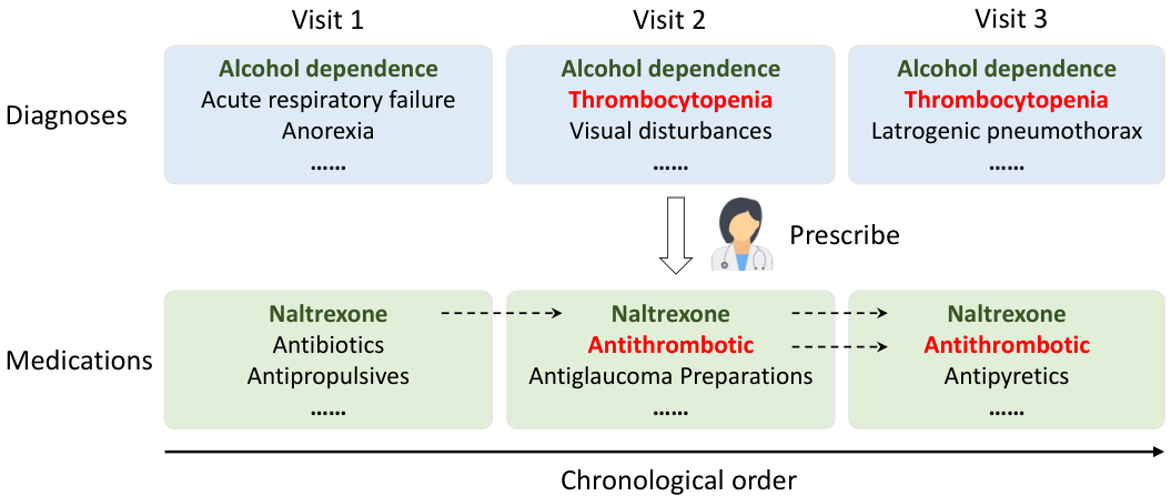
Medication recommendation aims to provide a set of medicines to treat the set of diagnosed diseases of a patient. Take the patient in Figure 1 for example, this patient visits the hospital for three times. In each visit, this patient is diagnosed with a set of diseases and is prescribed a set of medicines to treat these diseases. Currently, medication recommendation is mainly conducted by doctors according to their expertise and experiences. However, many patients are diagnosed with multiple diseases at one time. To conduct a considerate medication recommendation, on one hand, the doctor needs to select proper medicines for each disease; on the other hand, the doctor needs to avoid harmful drug-drug interactions (DDI) among selected medicines. Therefore, for complicated cases, medication recommendation is time-consuming for experienced doctors and error-prone for inexperienced doctors. To address this problem, the automatic medication recommendation that can assist doctors in decision making is urged.
Due to the clinical value, medication recommendation has attracted growing research interests. A series of deep learning based medication recommendation methods (Yang et al. 2021b; Yang et al. 2021a) have been proposed, which can be divided into two categories: Instance-based models (Zhang et al. 2017; Read et al. 2009; Gong et al. 2021) only use patient’s current diagnoses and procedures to conduct recommendations while ignoring the longitudinal patient history. In this manner, instance-based based models fail to consider the historical disease development process. To address this issue, Longitudinal models (Yang et al. 2021b; Shang et al. 2019; Yang et al. 2021a; Le et al. 2018) are designed to take use of the longitudinal patient history and capture the temporal dependencies. Existing longitudinal models usually consist of two stages, first aggregating the known information into a patient-level representation, and then conducting medication recommendation based on it.
One problem of existing works is that they do not explicitly model the relationship between medication recommendations for the same patient. However, in clinical practice, the recommendations for the same patients are closely related. For example, for patients with chronic diseases, they may keep using the same medicine all their lives. As shown in Figure 1, we conduct a statistical analysis on the MIMIC-III dataset. For each visit, we calculate the proportion of medications that have appeared in history and the Jaccard between current medications and past medications. We can see that in the most visits, a large portion of prescribed medicines have been recommended before. Inspired by this, we rethink about taking use of historical information from a medication-level perspective. The challenge here is how to accurately determine whether a historical medication is still relevant at present.
In this paper, we propose an encoder-decoder based generation network to produce the appropriate medications in a sequential manner, named Conditional Generation Net (COGNet). The proposed COGNet consists of the basic model and the copy module. The basic model conducts recommendation only based on patients’ health conditions in current visit; the copy module introduces the information of historical visits in modeling. Different from the basic model, in generating each medicine, the copy module decides whether to copy a medicine from historical recommendations or to predict a new one. The experiments on a public dataset demonstrate the effectiveness of the proposed model. We summarize our major contributions as follows:
- •
We propose a medication recommendation model, COGNet, which introduces a novel copy-or-predict mechanism. COGNet can leverage historical recommendations to produce a more accurate recommendation.
- •
We develop a novel hierarchical selection mechanism, which chooses the reusable medicines to copy from both medication-level and visit-level perspectives. This increases the intepretability of the proposed COGNet.
- •
We conduct comprehensive experiments on a public dataset MIMIC-III to demonstrate the effectiveness of the proposed COGNet.
2. Problem Formulation
2.1. Electrical Health Records (EHR)
The basic unit of EHR is patient and each patient consists of several visits. Let denote a longitudinal EHR of patients. Each patient has visited the hospital as least once and the -th patient can be represented as a sequence of multivariate observations . Here is the number of visits of the -th patient. To simplify the notation, we ignore the index and describe our methods with a single patient, then a patient is represented as . Let denotes the set of diagnoses, denotes the set of procedures and denotes the set of medications. , and indicate the number of all possible diagnoses, procedures and medications, respectively. Then, each visit of the patient can be represented by , where , and .
2.2. EHR&DDI Graph
and denote the EHR graph and DDI graph respectively, where is all the possible medication combinations in and is the known DDIs. Formally, we use the adjacency matrix to illustrate the construction of the graphs. means the -th and -th medications have appeared in the same visit. For , only the pair-wise DDIs are considered, means the -th and -th medications are mutually interacted. and are the same for all patients.
2.3. Medication Recommendation Problem
Given a patient’s current diagnoses , procedures , historical visit information , and the EHR and DDI graphs and , the goal is to train a model (i.e., COGNet) which can recommend the proper medication combination for this patient.
| Notation | Description |
|---|---|
| Electronic Health Records | |
| Record for a single patient | |
| Diagnoses, Procedure and Medication set | |
| EHR or DDI Graph | |
| Edge set and adjacency matrix of graph | |
| Origin embedding tables | |
| Graph embedding for medications |
3. Framework
Figure 3 illustrates the architecture of COGNet. We employ an encoder-decoder based generative network to generate the appropriate medication combination based on the patient’s current and historical health conditions. In the encoder, we encode all medical codes of the historical visits (i.e., ,,,) to represent the patient’s historical health conditions and encode the diagnosis and procedure codes of the th visit to represent the patient’s current health condition. In the decoder, we will generate the medication one by one to compose the recommendation drug combination. During each decoding step, the decoder combines the information of the diagnoses, procedures and generated medications to recommend the next medication. Moreover, if some diseases in current visit keep consistent with the past visits, the copy module will directly copy the corresponding medications from historical drug combinations. We will first describe the basic encoder-decoder based generation model and then address the copy module in detail in the following subsections.
3.1. Input Representations
We design three embedding tables, , and , where each row is an embedding vector for a distinct diagnosis code, procedure code or medication code. Here denotes the dimension of the embedding space. For each diagnosis set (), we first convert its every element to a -dimensional vector via the embedding matrix . Then, we can obtain the representation of the diagnosis set . For each procedure set () and medication set (), we can also obtain their representations and via the embedding matrices and , respectively.
3.2. Basic Model
In the basic model, we recommend the medication combination only based on the patient’s health condition in current visit. The basic model is an encoder-decoder generation model. It consists of four modules: diagnosis encoder, procedure encoder, medication graph encoder, and medication combination decoder.
3.2.1. Diagnosis Encoder
The diagnosis encoder aims to represent the patient’s health conditions based on the diagnosis codes. It is a Transformer-based (Vaswani et al. 2017) network and has the following two major sub-layers.
Multi-Head Self-Attention. This sub-layer aims to capture relations among all diagnoses in the same visit. Given three input matrices , and where , the attention function is defined as:
| (1) |
Multi-head attention layer will further project the input to multiple representation subspaces and capture the interaction information from multiple views (Qiu et al. 2021).
| (2) |
, , and are the parameters to learn. is the number of heads.
Position-wise Feed-Forward. This sub-layer consists of two linear projections with a ReLU activation in between.
| (3) |
where , , and are trainable parameters.
The diagnosis encoder then employs the residual connection and layer normalization function defined in (Ba et al. 2016) around the above two sub-layers to extract the diagnosis representation:
| (4) |
where is the diagnosis representation of the -th visit encoded by this encoder.
3.2.2. Procedure Encoder
The procedure encoder has the same network structure as the diagnosis encoder but their parameters are different. Through the same encoding process, we can also obtain the procedure representation via the procedure encoder:
| (5) |
3.2.3. Medication Graph Encoder
This encoder aims to model two kinds of drug relations:
- •
Medication EHR co-occurrence relationship: Some medications are often prescribed together for better efficacy. For example, ranitidine and sucralfate are the popular drug combination used to treat acute gastritis. Hence, modeling these co-occurrence relations can help the decoder to recommend the drug according to the partially generated medications.
- •
DDI: As mentioned above, some medications have the DDI and can not be used together. When recommending the drug, the decoder should avoid that it is conflict with the past recommended drugs. Hence, modeling this relation can help to recommend a safe and effective medication combination.
Inspired by (Shang et al. 2019), we use the Graph Convolutional Network (Kipf and Welling 2017) to model two kinds of relations based on the medication EHR and DDI graphs.
Given the input medication features and the medication graph adjacency matrix , the will obtain the new medication representations as follows:
| (6) |
, is the identity matrix and is the diagonal node degree matrix of (i.e., ).
First, we use a two-layer GCN to model the medication EHR co-occurrence relations based on the EHR graph adjacency matrix .
| (7) |
where is the learnable parameter.
Then, we use another two-layer GCN to model the DDI relations based on the DDI graph .
| (8) |
where is the learnable parameter.
Finally, we fuse two medication relation representations and to obtain the relation-aware medication representations.
| (9) |
where is a learnable parameter.
3.2.4. Medication Combination Decoder
The decoder will recommend the medication one by one for the th visit. For example, at the -th decoding step, the decoder will recommend the next medication based on the partially generated medication combination and the patient health conditions in the -th visit (i.e., and ). The decoding process is as follows.
First, we convert all generated medications to vectors via the original embedding matrix and relation representation matrix and can obtain two representations of the partially generated medication combination and . We fuse two representations to obtain the relation-aware medication combination representation.
| (10) |
Then, we use the multi-head self-attention mechanism (defined in Eq.(2)) to capture the interactions among the recommended medications.
| (11) |
Intuitively, the medication recommendation task aims to generate the recommendation of drugs that can cover all diseases of the patient. Thus, the patient’s disease and procedure representations and play an auxiliary role during the decoding process. To this end, we align the patient’s health conditions to adaptively model the uncovered diseases to guide the next medication recommendation.
| (12) |
Finally, we use the last row of (i.e., ) to predict the -th medication via an MLP layer.
| (13) |
where and are learnable parameters. denotes the probabilities of all medications in the vocabulary in which the medication with the maximum probability is the predicted medication at step .
3.3. Copy Module
In Basic Model section, we introduce the encoder-decoder based model to generate the medication recommendation results based on the patient’s current health conditions. It doesn’t consider the information of patient’s historical visits. In this section, we design a novel copy module to extend the basic model, which first compares the health conditions of current and historical visits and then copies the reusable medications to prescribe for current visit according to the condition changes.
Since the patient may have multiple visits, we use the hierarchical selection mechanism to conduct the copy process at each decoding step. First, we use the visit-level selection to pick a similar visit by comparing their health conditions. Then, at the specific decoding step, we use the medication-level selection to pick a particular medication from the prescriptions of the selected visit and add it to the recommendation results. Finally, we repeat the above process to copy the reusable medications iteratively to form the complete recommendation medication list. Note that the selection process is “soft” like the attention mechanism (Xu et al. 2015) and assigns different probabilities for all visits/medications to highlight the choice. We will take the -th medication recommendation of the -th visit (i.e., ) as an example to illustrate the copy process.
3.3.1. Visit-level Selection
We first uses two gated aggregation layers to encode the visit-level health conditions of all visits by aggregating their diagnosis and procedure representations, respectively:
| (14) |
| (15) |
where , , and are trainable parameters. Then we calculate the visit-level selection score of the past -th visit () by measuring the similarity between it and the current -th visit.
| (16) |
denotes the selection score of the -th visit.
3.3.2. Medication-level Selection
We use the hidden state formulated in Eq.(12), which comprehensively encodes the information of diagnoses, procedures and recommended medications, to determine which historical medications are reusable in current situation.
We firstly obtain the medication representations of all past visits through the similar process in Section 3.2.1:
| (17) |
where .
Then, we use the hidden state as the query vector to calculate the selection score along the medication dimension. The selection score of -th medication in -th visit ( and ) is
| (18) | |||
| (19) |
where is a learnable parameter. denotes the medication-level selection score.
3.3.3. Copy Mechanism
We combine the visit-level and medication-level scores to determine the copy probability of each medication in past visits. Moreover, since a medication may be used in multiple past prescriptions, we gather its final copy probability as follows:
| (20) | |||
| (21) |
where is an indicator function which returns 1 if , and 0 if . The copy probabilities of all medications is .
Finally, we combine the generation probabilities and copy probabilities to conduct the prediction.
| (22) | |||
| (23) |
where and are learnable parameters. denotes the probabilities of all medications in the medication set in which the medication with the maximum probability is the predicted -th medication of the th visit.
3.4. Training
We train the model by minimizing regular cross-entropy loss:
| (24) |
where is the training EHR set. is the -th medication of the medication set of the th visit. is the predicted probability of the and can be calculated by the Eq.(22). denotes all trainable parameters in COGNet.
During the training phase, we use the teacher-forcing to train the model. Specifically, when predicting the -th medication, the model takes the real -th medication rather than the predicted -th medication as the input of the decoder. At the first step, the input of the decoder is set to a special token .
| Model | Jaccard | F1 | PRAUC | DDI | Avg. # of Drugs |
|---|---|---|---|---|---|
| LR | 0.4865 0.0021 | 0.6434 0.0019 | 0.7509 0.0018 | 0.0829 0.0009 | 16.1773 0.0942 |
| ECC | 0.4996 0.0049 | 0.6569 0.0044 | 0.6844 0.0038 | 0.0846 0.0018 | 18.0722 0.1914 |
| RETAIN | 0.4887 0.0028 | 0.6481 0.0027 | 0.7556 0.0033 | 0.0835 0.0020 | 20.4051 0.2832 |
| LEAP | 0.4521 0.0024 | 0.6138 0.0026 | 0.6549 0.0033 | 0.0731 0.0008 | 18.7138 0.0666 |
| DMNC | 0.4864 0.0025 | 0.6529 0.0030 | 0.7580 0.0039 | 0.0842 0.0011 | 20.0000 0.0000 |
| GAMENet | 0.5067 0.0025 | 0.6626 0.0025 | 0.7631 0.0030 | 0.0864 0.0006 | 27.2145 0.1141 |
| MICRON | 0.5100 0.0033 | 0.6654 0.0031 | 0.7687 0.0026 | 0.0641 0.0007 | 17.9267 0.2172 |
| SafeDrug | 0.5213 0.0030 | 0.6768 0.0027 | 0.7647 0.0025 | 0.0589 0.0005 | 19.9178 0.1604 |
| COGNet | 0.5336 0.0011 | 0.6869 0.0010 | 0.7739 0.0009 | 0.0852 0.0005 | 28.0903 0.0950 |
| Item | Number |
|---|---|
| # of visits / # of patients | 14,995 / 6,350 |
| diag. / prod. / med. space size | 1,958 / 1430 / 131 |
| avg. / max # of visits | 2.37 / 29 |
| avg. / max # of diagnoses per visit | 10.51 / 128 |
| avg. / max # of procedures per visit | 3.84 / 50 |
| avg. / max # of medications per visit | 11.44 / 65 |
| total # of DDI pairs | 448 |
3.5. Inference
During the inference phase, inspired by the medication recommendation method (Zhang et al. 2017) and some NLP generation methods (Zhou et al. 2017; Nema et al. 2019; Qiu et al. 2020), we use the beam search trick to improve the performance. Different from the greedy search which only selects one best candidate as the partially generated medication combination for each decoding step, the beam search algorithm selects multiple alternatives at each decoding step based on conditional probability.
4. Experiments
In this section, we first introduce the experimental setups. Then we conduct some experiments to demonstrate the effectiveness of our COGNet model11 1 https://github.com/BarryRun/COGNet.
4.1. Dataset
We use the Medical Information Mart for Intensive Care (MIMIC-III)22 2 https://mimic.physionet.org/(Johnson et al. 2016) dataset released on PhysioNet. It contains a total of 46520 patients and 58976 hospital admissions from 2001 to 2012. For a fair comparison, we use the data processing script 33 3 https://github.com/ycq091044/SafeDrug released by (Yang et al. 2021b) and take the processed data as our benchmark. Details of the processing can be found in Appendix. Table 3 shows some statistics on the processed data.
4.2. Baselines and Metrics
We evaluate the performance of our approach by comparing it with several baseline methods.
- •
LR, standard Logistic Regression;
- •
ECC (Read et al. 2009), Ensemabled Classifier Chain, which uses a multi-hot vector to encode the diagnosis and procedure sets and leverage multiple SVM classifiers to make multi-label prediction;
- •
RETAIN (Choi et al. 2016), which uses the attention and gate mechanism to improve the prediction interpretability;
- •
LEAP (Zhang et al. 2017), which uses the LSTM based generation model to conduct medication recommendation based on the diagnose information;
- •
DMNC (Le et al. 2018), which proposes a new memory augmented neural network model to improve the patient encoder;
- •
GAMENet (Shang et al. 2019), which further combines the memory network and graph neural network to recommend the medication combinations;
- •
MICRON (Yang et al. 2021a), which first uses an recurrent residual learning model to predict the medication changes and then conducts medication recommendation based on the medication changes and the medication combination of the last visit;
- •
SafeDrug (Yang et al. 2021b), which combines the drug molecular graph and DDI graph to predict the safe medication combination.
Following the previous medication recommendation work (Shang et al. 2019; Yang et al. 2021b; Yang et al. 2021a), we use Jaccard Similarity Score (Jaccard), Average F1 (F1), Precision Recall AUC (PRAUC), and DDI Rate as our evaluation metrics. Each metric is averaged over all patients. The metric definitions can be found in Appendix.
| Model | Jaccard | F1 | PRAUC | DDI | Avg. # of Drugs |
|---|---|---|---|---|---|
| COGNet w/o Copy | 0.5163 0.0010 | 0.6713 0.0009 | 0.7637 0.0018 | 0.0842 0.0005 | 28.3139 0.0766 |
| COGNet w/o | 0.5119 0.0016 | 0.6629 0.0014 | 0.7588 0.0014 | 0.0813 0.0005 | 26.8944 0.0953 |
| COGNet w/o | 0.5306 0.0013 | 0.6836 0.0012 | 0.7706 0.0013 | 0.0840 0.0002 | 29.1076 0.0795 |
| COGNet w/o | 0.4937 0.0011 | 0.6496 0.0011 | 0.7443 0.0014 | 0.0887 0.0004 | 28.0519 0.0995 |
| COGNet w/o | 0.5117 0.0010 | 0.6669 0.0010 | 0.7625 0.0016 | 0.0831 0.0002 | 28.9554 0.0885 |
| COGNet w/o BS | 0.5266 0.0021 | 0.6805 0.0019 | 0.7729 0.0013 | 0.0840 0.0004 | 28.5592 0.0701 |
| COGNet | 0.5336 0.0011 | 0.6869 0.0010 | 0.7739 0.0009 | 0.0852 0.0005 | 28.0903 0.0950 |
4.3. Result Analysis
4.3.1. Overall Comparison
Table 2 shows the results of all methods. Overall, our proposed model COGNet outperforms all baselines with the higher Jaccard, F1 and PRAUC. The performances of LR, ECC and LEAP are poor as they are instance-based models that only consider the diagnoses and procedures in the current visit. RETAIN, DMNC, GAMENet, SafeDrug and MICRON perform relatively better because they preserve longitudinal patient information in different ways. RETAIN and DMNC only encode the patients’ historical information, while GAMENet introduces additional graph information and SafeDrug incorporates the drug molecule structures in medication recommendation, resulting in a further performance improvement. MICRON also notices that some medications in the current visit keeps consistent with the last visit and uses the recurrent residual method to inherit the unchanged part. However, it fails to consider the correlations among the recommended medications and the recurrent like method is hard to model the long range visit information. Hence, COGNet performs better than MICRON. SafeDrug achieves a lower DDI rate by introducing the additional drug molecule information. However, the MIMIC-III dataset itself has an average DDI of 0.08379 and our COGNet has a similar performance. It suggests that COGNet mimics the behavior of physicians in prescribing medications well.
4.3.2. Effect of number of visits
To further explore whether our COGNet can better capture historical medication information, we investigate the impact of the number of visits on the performance of different models. Since most patients in MIMIC visit the hospital less than five times, we take the first five visits for each patient in the test set to conduct the analysis. As a comparison, we also take the two strongest baselines SafeDrug and MICRON, which also incorporate historical information, to conduct the analysis. Figure 4 shows the results. We can see that COGNet achieves relatively better performance with more visits, while the performance of SafeDrug almost stays flat and MICRON shows a decreasing trend. The reason may be that COGNet uses the attention based hierarchical selection mechanism, which can more effectively incorporate the information of past visits than RNN like mechanism used in SafeDrug. Moreover, MICRON iteratively updates the past medication combination to form the new medication set, which will be affected by the error accumulation problem.
4.4. Ablation Study
To verify the effectiveness of each module of COGNet, we design the following ablation models:
- •
COGNet w/o Copy: We remove the copy module, which means changing the Eq.(22) to .
- •
COGNet w/o : We maintain the copy module but remove the visit-level selection by changing the in Eq.(21) to .
- •
COGNet w/o : We remove the EHR and DDI graphs in decoder, which means changing the Eq.(10) to .
- •
COGNet w/o : We remove the diagnoses information in each visit.
- •
COGNet w/o : We remove the procedures information in each visit.
- •
COGNet w/o BS. We use the greedy search strategy in the inference phase rather than beam search.
Table 4 shows the results for the different variants of COGNet. As expected, the results of COGNet w/o Copy indicate that the copy mechanism brings a significant improvement to the basic model. COGNet can improve the medication recommendation by replicating historical drugs. COGNet w/o illustrates the effectiveness of visit-level selection scores.
Both COGNet w/o and COGNet w/o yield poor results among all ablation models, which suggest that diagnosis and procedure information play a great role in medication recommendation. The results of COGNet w/o and COGNet w/o BS indicate that graphs and beam search also have contributions to the final result. Overall, the complete COGNet outperforms all ablation models, which means each component of our model is integral.

4.5. Case Study
We present an example patient in MIMIC-III to illustrate how COGNet conducts the copy mechanism to improve medication recommendation. This patient visited the hospital twice. At the first time, the patient was mainly diagnosed with pneumonia, septicemia, sepsis, etc. Later, the patient returned for a second visit. In addition to the previously diagnosed diseases, the patient also had some new diseases, like gastroesophageal laceration and gastric ulcer. The table in Fig 5 shows the details. Due to space constraints, we use International Classification of Diseases (ICD)44 4 http://www.icd9data.com/ codes to represent diagnosis results and Anatomical Therapeutic Chemical (ATC)55 5 https://www.whocc.no/atc/structure_and_principles/ classification system to represent medications.
As shown in Figure 5, we visualize the copy probability computed by Eq.(20) at each decoding step of recommending the medications for the second visit. We can see that some reusable medications, like A11D, N07B and H03A, are correctly copied by assigning high probabilities to them in previous visit. In addition, some new drugs, like J01C and R03A, can also be appropriately generated. It indicates that COGNet can not only copy historical drugs according to unhealed diseases, but also generate new drugs based on new diagnosis results. The visualization results also hint that COGNet can provide a good way for the interpretation of the medication recommendation process.
5. Related Work
5.1. Medication Recommendation
Due the clinical value, medication recommendation has received increasing attention in recent years. According to the used information, existing approaches can be broadly categorized into rule-based, instance-based, and longitudinal methods.
5.1.1. Rule-based Methods
Rule-based methods (Almirall et al. 2012; Chen et al. 2016; Gunlicks-Stoessel et al. 2016; Lakkaraju and Rudin 2017) rely on the human-designed recommendation protocols. For example, Gunlicks-Stoessel et al. (Gunlicks-Stoessel et al. 2016) attempts to recommend porper treatments for adolescent depression based on rules. However, these methods require a lot of effort from clinicians and lack generalization.
5.1.2. Instance-based Methods
Instance-based methods (Zhang et al. 2017; Gong et al. 2021) only take the information of current visit as input. For example, Zhang et al. (Zhang et al. 2017) firstly encode the patient’s current diagnose and then use a recurrent decoder to generate the medication recommendations based on the encoded information. However, they ignore the historical visit information of the patient.
5.1.3. Longitudinal Methods
These approaches (Wang et al. 2018; Wang et al. 2019; Shang et al. 2019; Yang et al. 2021a; Yang et al. 2021b; Bhoi et al. 2020) use the historical information of patients and explore the sequential dependency between visits. Most of them basically model the longitudinal patient information by RNNs. Le et al. (Le et al. 2018) and Shang et al. (Shang et al. 2019) combine memory networks with RNNs to enhance the memory ability. Yang et al. (Yang et al. 2021b) further incorporate the drugs’ molecule information to improve the medication representation learning. Yang et al. (Yang et al. 2021a) explicitly model the health condition changes of the patient to enhance the correlations between continuous visits by a recurrent residual learning approach. However, these methods do not explicitly consider the relationship between the medication recommendations of the same patient and the RNN like methods are hard to handle the long range visit dependency.
5.2. Graph Neural Network
Recently, graph neural networks (GNN) (Kipf and Welling 2017; Zhuang and Ma 2018; Hamilton et al. 2017; Atwood and Towsley 2016; Velickovic et al. 2018; Vasile et al. 2016) have received wide attention in many fields. The convolutional GNN can learn powerful node representations by aggregating the neighbors’ features over the graph. Some works (Shang et al. 2019; Yang et al. 2021b) have attempted to leverage the GNN to improve the medication recommendation. For example, Yang et al. (Yang et al. 2021b) take the drugs’ molecule structures as graphs and use GNN to learn the better medication representations to improve medication recommendation. Shang et al. (Shang et al. 2019) use the GNN to encode the EHR and DDI graphs to introduce the medication correlation information. In this paper, inspired by (Shang et al. 2019), we use the GNN to encode the medication co-occurrence and DDI relationships to improve the recommendation.
6. Conclusion
In this paper, we proposed a novel medication recommendation model, COGNet, to better leverage historical information from a medication-level perspective. COGNet works under an encoder-decoder based framework and introduces a copy-or-predict mechanism to accurately determine whether a historical medication is still relevant at present. Experiment results on the publicly available MIMIC-III dataset demonstrate that COGNet outperforms existing medication recommendation methods. We also investigate the impact of number of visits on the performance, which shows that COGNet can effectively incorporate the information of multiple past visits. Further ablation study results also suggest the effectiveness of each module of COGNet.
Acknowledgements.
This work was supported by National Key R&D Program of China, No. 2018YFC0117000. This work was also partially supported by Natural Science Foundation of China grant, No. U21A20488.References
- (1)
- Almirall et al. (2012) Daniel Almirall, Scott N Compton, Meredith Gunlicks-Stoessel, Naihua Duan, and Susan A Murphy. 2012. Designing a pilot sequential multiple assignment randomized trial for developing an adaptive treatment strategy. Statistics in medicine 31, 17 (2012), 1887–1902.
- Atwood and Towsley (2016) James Atwood and Don Towsley. 2016. Diffusion-Convolutional Neural Networks. In Advances in Neural Information Processing Systems 29: Annual Conference on Neural Information Processing Systems 2016, December 5-10, 2016, Barcelona, Spain, Daniel D. Lee, Masashi Sugiyama, Ulrike von Luxburg, Isabelle Guyon, and Roman Garnett (Eds.). 1993–2001. https://proceedings.neurips.cc/paper/2016/hash/390e982518a50e280d8e2b535462ec1f-Abstract.html
- Ba et al. (2016) Jimmy Lei Ba, Jamie Ryan Kiros, and Geoffrey E. Hinton. 2016. Layer Normalization. arXiv:1607.06450 [cs.LG]
- Bhoi et al. (2020) Suman Bhoi, Mong-Li Lee, and Wynne Hsu. 2020. PREMIER: Personalized REcommendation for Medical prescrIptions from Electronic Records. CoRR abs/2008.13569 (2020). arXiv:2008.13569 https://arxiv.org/abs/2008.13569
- Chen et al. (2016) Zhuo Chen, Kyle Marple, Elmer Salazar, Gopal Gupta, and Lakshman Tamil. 2016. A Physician Advisory System for Chronic Heart Failure management based on knowledge patterns. Theory Pract. Log. Program. 16, 5-6 (2016), 604–618. https://doi.org/10.1017/S1471068416000429
- Choi et al. (2016) Edward Choi, Mohammad Taha Bahadori, Jimeng Sun, Joshua Kulas, Andy Schuetz, and Walter F. Stewart. 2016. RETAIN: An Interpretable Predictive Model for Healthcare using Reverse Time Attention Mechanism. In Advances in Neural Information Processing Systems 29: Annual Conference on Neural Information Processing Systems 2016, December 5-10, 2016, Barcelona, Spain, Daniel D. Lee, Masashi Sugiyama, Ulrike von Luxburg, Isabelle Guyon, and Roman Garnett (Eds.). 3504–3512. https://proceedings.neurips.cc/paper/2016/hash/231141b34c82aa95e48810a9d1b33a79-Abstract.html
- Gong et al. (2021) Fan Gong, Meng Wang, Haofen Wang, Sen Wang, and Mengyue Liu. 2021. SMR: Medical Knowledge Graph Embedding for Safe Medicine Recommendation. Big Data Res. 23 (2021), 100174. https://doi.org/10.1016/j.bdr.2020.100174
- Gunlicks-Stoessel et al. (2016) Meredith Gunlicks-Stoessel, Laura Mufson, Ana Westervelt, Daniel Almirall, and Susan Murphy. 2016. A pilot SMART for developing an adaptive treatment strategy for adolescent depression. Journal of Clinical Child & Adolescent Psychology 45, 4 (2016), 480–494.
- Hamilton et al. (2017) William L. Hamilton, Zhitao Ying, and Jure Leskovec. 2017. Inductive Representation Learning on Large Graphs. In Advances in Neural Information Processing Systems 30: Annual Conference on Neural Information Processing Systems 2017, December 4-9, 2017, Long Beach, CA, USA, Isabelle Guyon, Ulrike von Luxburg, Samy Bengio, Hanna M. Wallach, Rob Fergus, S. V. N. Vishwanathan, and Roman Garnett (Eds.). 1024–1034. https://proceedings.neurips.cc/paper/2017/hash/5dd9db5e033da9c6fb5ba83c7a7ebea9-Abstract.html
- Johnson et al. (2016) Alistair E. W. Johnson, Tom J. Pollard, Lu Shen, Li wei H. Lehman, Mengling Feng, Mohammad Mahdi Ghassemi, Benjamin Moody, Peter Szolovits, Leo Anthony Celi, and Roger G. Mark. 2016. MIMIC-III, a freely accessible critical care database. Scientific Data 3 (2016).
- Kingma and Ba (2015) Diederik P. Kingma and Jimmy Ba. 2015. Adam: A Method for Stochastic Optimization. In 3rd International Conference on Learning Representations, ICLR 2015, San Diego, CA, USA, May 7-9, 2015, Conference Track Proceedings, Yoshua Bengio and Yann LeCun (Eds.). http://arxiv.org/abs/1412.6980
- Kipf and Welling (2017) Thomas N. Kipf and Max Welling. 2017. Semi-Supervised Classification with Graph Convolutional Networks. In 5th International Conference on Learning Representations, ICLR 2017, Toulon, France, April 24-26, 2017, Conference Track Proceedings. OpenReview.net. https://openreview.net/forum?id=SJU4ayYgl
- Lakkaraju and Rudin (2017) Himabindu Lakkaraju and Cynthia Rudin. 2017. Learning Cost-Effective and Interpretable Treatment Regimes. In Proceedings of the 20th International Conference on Artificial Intelligence and Statistics, AISTATS 2017, 20-22 April 2017, Fort Lauderdale, FL, USA (Proceedings of Machine Learning Research, Vol. 54), Aarti Singh and Xiaojin (Jerry) Zhu (Eds.). PMLR, 166–175. http://proceedings.mlr.press/v54/lakkaraju17a.html
- Le et al. (2018) Hung Le, Truyen Tran, and Svetha Venkatesh. 2018. Dual Memory Neural Computer for Asynchronous Two-view Sequential Learning. In Proceedings of the 24th ACM SIGKDD International Conference on Knowledge Discovery & Data Mining, KDD 2018, London, UK, August 19-23, 2018, Yike Guo and Faisal Farooq (Eds.). ACM, 1637–1645. https://doi.org/10.1145/3219819.3219981
- Nema et al. (2019) Preksha Nema, Akash Kumar Mohankumar, Mitesh M. Khapra, Balaji Vasan Srinivasan, and Balaraman Ravindran. 2019. Let’s Ask Again: Refine Network for Automatic Question Generation. In Proceedings of the 2019 Conference on Empirical Methods in Natural Language Processing and the 9th International Joint Conference on Natural Language Processing, EMNLP-IJCNLP 2019, Hong Kong, China, November 3-7, 2019, Kentaro Inui, Jing Jiang, Vincent Ng, and Xiaojun Wan (Eds.). Association for Computational Linguistics, 3312–3321. https://doi.org/10.18653/v1/D19-1326
- Qiu et al. (2020) Zhaopeng Qiu, Xian Wu, and Wei Fan. 2020. Automatic Distractor Generation for Multiple Choice Questions in Standard Tests. In COLING. International Committee on Computational Linguistics, 2096–2106.
- Qiu et al. (2021) Zhaopeng Qiu, Xian Wu, Jingyue Gao, and Wei Fan. 2021. U-BERT: Pre-training User Representations for Improved Recommendation. In AAAI. AAAI Press, 4320–4327.
- Read et al. (2009) Jesse Read, Bernhard Pfahringer, Geoffrey Holmes, and Eibe Frank. 2009. Classifier Chains for Multi-label Classification. In Machine Learning and Knowledge Discovery in Databases, European Conference, ECML PKDD 2009, Bled, Slovenia, September 7-11, 2009, Proceedings, Part II (Lecture Notes in Computer Science, Vol. 5782), Wray L. Buntine, Marko Grobelnik, Dunja Mladenic, and John Shawe-Taylor (Eds.). Springer, 254–269. https://doi.org/10.1007/978-3-642-04174-7_17
- Shang et al. (2019) Junyuan Shang, Cao Xiao, Tengfei Ma, Hongyan Li, and Jimeng Sun. 2019. GAMENet: Graph Augmented MEmory Networks for Recommending Medication Combination. In The Thirty-Third AAAI Conference on Artificial Intelligence, AAAI 2019, The Thirty-First Innovative Applications of Artificial Intelligence Conference, IAAI 2019, The Ninth AAAI Symposium on Educational Advances in Artificial Intelligence, EAAI 2019, Honolulu, Hawaii, USA, January 27 - February 1, 2019. AAAI Press, 1126–1133. https://doi.org/10.1609/aaai.v33i01.33011126
- Tatonetti et al. (2012) Nicholas P Tatonetti, P Ye Patrick, Roxana Daneshjou, and Russ B Altman. 2012. Data-driven prediction of drug effects and interactions. Science translational medicine 4, 125 (2012), 125ra31–125ra31.
- Vasile et al. (2016) Flavian Vasile, Elena Smirnova, and Alexis Conneau. 2016. Meta-Prod2Vec: Product Embeddings Using Side-Information for Recommendation. In RecSys. ACM, 225–232.
- Vaswani et al. (2017) Ashish Vaswani, Noam Shazeer, Niki Parmar, Jakob Uszkoreit, Llion Jones, Aidan N. Gomez, Lukasz Kaiser, and Illia Polosukhin. 2017. Attention is All you Need. In Advances in Neural Information Processing Systems 30: Annual Conference on Neural Information Processing Systems 2017, December 4-9, 2017, Long Beach, CA, USA, Isabelle Guyon, Ulrike von Luxburg, Samy Bengio, Hanna M. Wallach, Rob Fergus, S. V. N. Vishwanathan, and Roman Garnett (Eds.). 5998–6008. https://proceedings.neurips.cc/paper/2017/hash/3f5ee243547dee91fbd053c1c4a845aa-Abstract.html
- Velickovic et al. (2018) Petar Velickovic, Guillem Cucurull, Arantxa Casanova, Adriana Romero, Pietro Liò, and Yoshua Bengio. 2018. Graph Attention Networks. In 6th International Conference on Learning Representations, ICLR 2018, Vancouver, BC, Canada, April 30 - May 3, 2018, Conference Track Proceedings. OpenReview.net. https://openreview.net/forum?id=rJXMpikCZ
- Wang et al. (2018) Lu Wang, Wei Zhang, Xiaofeng He, and Hongyuan Zha. 2018. Supervised Reinforcement Learning with Recurrent Neural Network for Dynamic Treatment Recommendation. In Proceedings of the 24th ACM SIGKDD International Conference on Knowledge Discovery & Data Mining, KDD 2018, London, UK, August 19-23, 2018, Yike Guo and Faisal Farooq (Eds.). ACM, 2447–2456. https://doi.org/10.1145/3219819.3219961
- Wang et al. (2019) Shanshan Wang, Pengjie Ren, Zhumin Chen, Zhaochun Ren, Jun Ma, and Maarten de Rijke. 2019. Order-free Medicine Combination Prediction with Graph Convolutional Reinforcement Learning. In Proceedings of the 28th ACM International Conference on Information and Knowledge Management, CIKM 2019, Beijing, China, November 3-7, 2019, Wenwu Zhu, Dacheng Tao, Xueqi Cheng, Peng Cui, Elke A. Rundensteiner, David Carmel, Qi He, and Jeffrey Xu Yu (Eds.). ACM, 1623–1632. https://doi.org/10.1145/3357384.3357965
- Xu et al. (2015) Kelvin Xu, Jimmy Ba, Ryan Kiros, Kyunghyun Cho, Aaron C. Courville, Ruslan Salakhutdinov, Richard S. Zemel, and Yoshua Bengio. 2015. Show, Attend and Tell: Neural Image Caption Generation with Visual Attention. In Proceedings of the 32nd International Conference on Machine Learning, ICML 2015, Lille, France, 6-11 July 2015 (JMLR Workshop and Conference Proceedings, Vol. 37), Francis R. Bach and David M. Blei (Eds.). JMLR.org, 2048–2057. http://proceedings.mlr.press/v37/xuc15.html
- Yang et al. (2021a) Chaoqi Yang, Cao Xiao, Lucas Glass, and Jimeng Sun. 2021a. Change Matters: Medication Change Prediction with Recurrent Residual Networks. In Proceedings of the Thirtieth International Joint Conference on Artificial Intelligence, IJCAI 2021, Virtual Event / Montreal, Canada, 19-27 August 2021, Zhi-Hua Zhou (Ed.). ijcai.org, 3728–3734. https://doi.org/10.24963/ijcai.2021/513
- Yang et al. (2021b) Chaoqi Yang, Cao Xiao, Fenglong Ma, Lucas Glass, and Jimeng Sun. 2021b. SafeDrug: Dual Molecular Graph Encoders for Safe Drug Recommendations. CoRR abs/2105.02711 (2021). arXiv:2105.02711 https://arxiv.org/abs/2105.02711
- Zhang et al. (2017) Yutao Zhang, Robert Chen, Jie Tang, Walter F. Stewart, and Jimeng Sun. 2017. LEAP: Learning to Prescribe Effective and Safe Treatment Combinations for Multimorbidity. In Proceedings of the 23rd ACM SIGKDD International Conference on Knowledge Discovery and Data Mining, Halifax, NS, Canada, August 13 - 17, 2017. ACM, 1315–1324. https://doi.org/10.1145/3097983.3098109
- Zhou et al. (2017) Qingyu Zhou, Nan Yang, Furu Wei, Chuanqi Tan, Hangbo Bao, and Ming Zhou. 2017. Neural Question Generation from Text: A Preliminary Study. In NLPCC (Lecture Notes in Computer Science, Vol. 10619). Springer, 662–671.
- Zhuang and Ma (2018) Chenyi Zhuang and Qiang Ma. 2018. Dual Graph Convolutional Networks for Graph-Based Semi-Supervised Classification. In Proceedings of the 2018 World Wide Web Conference on World Wide Web, WWW 2018, Lyon, France, April 23-27, 2018, Pierre-Antoine Champin, Fabien Gandon, Mounia Lalmas, and Panagiotis G. Ipeirotis (Eds.). ACM, 499–508. https://doi.org/10.1145/3178876.3186116
Appendix A Additional Experimental Setups
A.1. Dataset Processing
In this section, we elaborate the operation of data processing. The original data is from “ADMISSIONS.csv”, “DIAGNOSES_ICD.csv“, “PROCEDURES_ICD.csv“ and ”PRESCRIPTIONS.csv“ files from the 1.40 version MIMIC-III. These tables are merged through admission id and subject id ("Admission" has the same meaning as "Visit" in this paper). We utilized all the patients with at least 2 visits. We prepared the available medications by retaining the top 300 medications in terms of number of occurrences. This is to improve the training speed for easier analysis. We extracted Top-40 severity DDI types from TWOSIDES (Tatonetti et al. 2012), which are reported by ATC Third Level codes. In order to be able to compute DDI score, we transform the NDC drug codes to same ATC level codes. After the above operation was completed, we divided the data into training, validation and test by the ratio of . We counted the frequency of all drug occurrences on the training set,and then resort the medications in ascending order by frequency for all patients.
A.2. Implementation Details
Our method is implemented by PyTorch 1.9.0 based on python 3.9.6, tested on an Intel Xeon 8255C machine with 315G RAM and 8 NVIDIA Tesla V100 GPUs. We choose the optimal hyperparameters based on the validation set, where the dimension size , number of beam search states is 4 and maximum generation length is 45. Models are trained on Adam optimizer (Kingma and Ba 2015) with learning rate and batch size 16 for 50 epochs. We fixed the random seed as 1203 for PyTorch to ensure the reproducibility of the models. During the test process, for a fair comparison, we apply bootstrapping sampling instead of cross-validation according to (Yang et al. 2021b). Precisely, we random sample data from test set for a round of evaluation and the results of 10 rounds are used to calculate the mean and standard deviation, which are finally reported. As the sampling process is random, the final experimental results may vary slightly.
A.3. Metrics
In this section, we present the definition of each metric used in the experiment section.
- •
Jaccard for a patient is calculated as below:
(25) where is the ground-truth medication combination and is the predicted result.
- •
F1 is the harmonic mean of precision and recall. For a patient, it is calculated as follows:
(26) (27) (28) - •
PRAUC refers to Precision Recall Area Under Curve. To compute PRAUC, each medication should correspond to a probability to be recommended (Yang et al. 2021b). However, since we model the medication recommendation as a sequential generation problem, it means that each medication will have a probability at every generation step. To resolve this issue, we adopt the following methods. For each recommended medications, we directly take the probability corresponding to the step in which they are recommended. For the other medications, we take the average of probabilities at all steps. Then the PRAUC can be calculated by
(29) where is the rank in the sequence of drugs. is the precision at cut-off in ordered retrieval list, and is the change in recall when deriving the -th drug.
- •
DDI measure the interaction between the recommended medications, which is calculated by:
(30) where is the adjacency matrix of DDI graph defined in section 4, denoted the -th recommended medication and is a function that return 1 when expression in is true, otherwise 0.
Appendix B Additional Experiments
B.1. Performance with Different Label Order
Since new medications are recommended under the conditions of already recommended medications, the relative order of the medications may have an impact on the final results. To explore which kind of sequencing would be more appropriate of medication recommendation, we conduct four different heuristics to order the data:
- •
Rare first ranks medications by their frequencies in the training data, placing the those that appear less frequently first.
- •
Frequent first put frequent medications before more rare medications.
- •
Early first sorts medications by chronological order, with those used earlier placed first.
- •
Late first arranges the medications in reverse chronological order.
Fig 6 shows the performance of COGNet with different ordering heuristics over training epochs. Rare first outperform the alternative labeling strategies, because it allows the model to focus more on unusual medications, thereby alleviating the data imbalance problem. Frequent first converges faster but performs poorly. The main reason is that the recommended medications are predominated by non-informative popular medications. The final results of Early first and Late first are weak, which indicates that chronological order is not a good choice in this task. In addition, we tried to randomly disrupt all the drugs, which is far worse than the above heuristics, so we do not show it.