跳到论文正文
W Papers独立论文阅读器 arXiv:2202.06392 论文正文 计算阅读时间 · 0%
引用这篇论文根据当前论文元数据生成,正式投稿前建议核对。


License: arXiv.org perpetual non-exclusive license
arXiv:2202.06392v2 [math.NA] 01 Dec 2022

Local approximation of operators

H. N. Mhaskar Thanks:  Institute of Mathematical Sciences, Claremont Graduate University, Claremont, CA 91711. email: hrushikesh.mhaskar@cgu.edu. The research is supported in part by NSF grant DMS 2012355 and ARO Grant W911NF2110218.
Abstract

Many applications, such as system identification, classification of time series, direct and inverse problems in partial differential equations, and uncertainty quantification lead to the question of approximation of a non-linear operator between metric spaces 𝔛\mathfrak{X} and 𝔜\mathfrak{Y}. We study the problem of determining the degree of approximation of such operators on a compact subset K𝔛⊂𝔛K_{\mathfrak{X}}\subset\mathfrak{X} using a finite amount of information. If ℱ:K𝔛→K𝔜\mathcal{F}:K_{\mathfrak{X}}\to K_{\mathfrak{Y}}, a well established strategy to approximate ℱ⁡(F)\mathcal{F}(F) for some F∈K𝔛F\in K_{\mathfrak{X}} is to encode FF (respectively, ℱ⁡(F)\mathcal{F}(F)) in terms of a finite number dd (repectively mm) of real numbers. Together with appropriate reconstruction algorithms (decoders), the problem reduces to the approximation of mm functions on a compact subset of a high dimensional Euclidean space ℝd{\mathbb{R}}^{d}, equivalently, the unit sphere 𝕊d{\mathbb{S}}^{d} embedded in ℝd+1{\mathbb{R}}^{d+1}. The problem is challenging because dd, mm, as well as the complexity of the approximation on 𝕊d{\mathbb{S}}^{d} are all large, and it is necessary to estimate the accuracy keeping track of the inter-dependence of all the approximations involved. In this paper, we establish constructive methods to do this efficiently; i.e., with the constants involved in the estimates on the approximation on 𝕊d{\mathbb{S}}^{d} being 𝒪⁡(d1/6){\cal O}(d^{1/6}). We study different smoothness classes for the operators, and also propose a method for approximation of ℱ⁡(F)\mathcal{F}(F) using only information in a small neighborhood of FF, resulting in an effective reduction in the number of parameters involved. To further mitigate the problem of large number of parameters, we propose prefabricated networks, resulting in a substantially smaller number of effective parameters. The problem is studied in both deterministic and probabilistic settings.

Keywords: Approximation of operators, zonal function networks, approximation on high dimensional spheres.

AMS Classification 2000: 41A25, 41A63, 42C10.

1 Introduction

While much of approximation theory deals with the question of approximation of functions on subsets of a Euclidean space, many applications require an approximation of non-linear functionals and even non-linear operators defined on compact subsets of function spaces. We give a few examples here; many more are listed in the references cited in Section 2.

  1. 1.

    In system identification problems, the hidden states of a non-linear system are not known, but need to be modeled using observations of the input-output relationships of the system (e.g., [46, 20]). Both the input signals and the output signals are functions of time, and the model is thus an unknown non-linear operator which needs to be approximated.

  2. 2.

    In prediction of time series, a time series (tℓ)ℓ=0∞(t_{\ell})_{\ell=0}^{\infty} is modeled by a functional relationship

    tℓ+q=F(tℓ,⋯,tℓ+q−1),ℓ=0,1,⋯,t_{\ell+q}=F(t_{\ell},\cdots,t_{\ell+q-1}),\qquad\ell=0,1,\cdots,

    for a judiciously chosen qq, where FF is some possibly non-linear function (e.g., [46, 39]). In order to use such a model for classification of time series, different time series are modeled by different functions FF, so that the class label is a non-linear functional on a class of functions.

  3. 3.

    In the theory of non-linear partial differential equations (PDEs), the mapping from the initial/boundary conditions to the solution or in the case of inverse problems, from the solution to the initial/boundary conditions or the coefficient functions in the differential equations are all non-linear operators.

  4. 4.

    In uncertainty quantification problems, the coefficients of the PDEs are random functions of the variables, and one is interested in some quantity of interest (e.g., [4]). Clearly, the quantity of interest is a possibly non-linear functional on the space of functions involved.

An obvious and natural way to solve such problems is to encode the input functions as well as output functions using finitely many parameters, and treat the problem as a problem of approximation of functions between finite dimensional Euclidean spaces. For example, a time series can be encoded in a variety of ways, such as thresholded PCA components of snippets [26], values of the empirical mode decomposition at certain points [27], parameters of an ARMA model [59], etc. In the context of PDEs, the input and output functions can be encoded using values of the functions involved [24], coefficients with respect to certain frames/bases [9], random features [16], etc. Clearly, any encoder needs to be associated with a decoder which can approximate the input and output functions well11 1 An encoder is referred to also as a parameter selection, feature map, or information operator. A decoder is referred to also as approximation operator, or reconstruction algorithm.. The exact nature of the encoder and decoder need to depend upon the specific application, but it is clear intuitively that the number of parameters defined by the encoders must be very large in order for the corresponding decoders to achieve a good approximation. Therefore, even though the idea behind the reduction to the problem of operator approximation to that approximation of functions between Euclidean spaces is obvious, the dimensions of these spaces poses a formidable problem. In this paper, we assume that the appropriate encoder/decoder pairs have been selected, and focus on the technical problems arising from the high dimensionality of the Euclidean spaces to which the parameters generated/desired by the encoders belong. We will discuss the issues involved in Section 3.1.

After pointing out a few papers related to the current paper in Section 2, we will formalize in Section 3 the intuitive thinking just described in an abstract manner. We will explain there how the problem can be reduced to the problem of efficient approximation of functions on a high dimensional sphere, and highlight the technical contributions of the current paper. In the rest of the paper, we will focus on approximation on a high dimensional sphere. In Section 4, we will review some preparatory material required both to formulate our results and to prove them. In Section 5, we will formulate our main theorems about approximation on the sphere. In Section 6, we illustrate an example on the application of our theory for approximation of operators defined on the space of continuous functions on a smooth, compact, Riemannian manifold. The proofs of all the new results in this paper are given in Section 7. In Appendix A, we make some comments on a possible computational scheme for the kernels introduced in Section 4.4. In Appendix B, we give another example to illustrate a certain technical point which could not be commented upon in the main part of the paper.

2 Related work

An early and widely cited work on the problem of functional/operator approximation is the paper [3] by Chen and Chen. They consider approximation by neural networks for nonlinear operators using what is sometimes called trunk and branch networks. First, one obtains an approximation of ℱ⁡(F)​(y)≈∑kβk​(F)​τk​(y)\mathcal{F}(F)(y)\approx\sum_{k}\beta_{k}(F)\tau_{k}(y), where τk\tau_{k} is a basis for range space of ℱ\mathcal{F}. The trunk networks are neural network approximations to τk\tau_{k}, and the branch networks approximate the coefficients βk​(F)\beta_{k}(F). In turn, each branch network is a composition of two networks, one to approximate FF and one to approximate βk\beta_{k} as a function of the parameters of the network to approximate FF. The authors prove universal approximation theorems for the resulting networks. While this approach is adequate for universal approximation theorems, it introduces extra error terms due to the approximation of ℱ⁡(F)\mathcal{F}(F) in the indicated format (see Appendix B).

From the point of view of system identification, the problem was studied already in early works of Sandberg [53, 52], Modha and Hecht-Nielsen [44], Dingankar [8], among others. This work motivated our own work [36].

In [36], we have taken a simpler approach than that of [3] for the approximation of nonlinear functionals (such as βk\beta_{k}) on spaces of the form Lp​([−1,1]s)L^{p}([-1,1]^{s}). We have constructed networks with a single hidden layer by considering the functional as a function of the coefficients of FF in a tensor product Legendre polynomial series. We have proved estimates on the degree of approximation in terms of the size of the networks, and proved that they are optimal in the sense of non-linear widths. The current paper is a substantial generalization and refinement of this work. The paper [55] obtains results similar to those in [36] in the case when the activation function is an ReLU function.

The problem of approximation of functions of infinitely many variables, especially on tensor product domains has a long history of research in the information based complexity community - there are too many papers in the Journal of Complexity alone to give a reasonably good bibliography. A detailed treatment from this point of view can be found in the series of books by Novak and Woźniakowski [49]. We point out only two recent papers. In [60], Werschulz and Woźniakowski study the tractability of approximating solutions of Volterra equations in high dimensions. In [18], Kritzer, Pillichshammer, and Woźniakowski study the tractability of approximation of operators between tensor product weighted Hilbert spaces.

In the last couple of years, a great deal of interest in this direction is triggered by possible applications to the solutions of direct and inverse problems involving partial differential equations (PDEs). For example, in [21, 47] the authors introduce the concept of Fourier neural networks, and examime the feature selection and training algorithms for solutions of PDEs. The paper [16] establishes a universal approximation theorem for deep networks in the topology of uniform convergence on compact sets using Hilbert space norms. This paper has a long list of related papers and the correspondingly long discussion. Universal approximation property for deep networks is established also in [15, 6], where the rates of convergence are studied for special PDEs. The paper [19] follows the approach of Chen and Chen, approximating the functionals βk​(F)\beta_{k}(F) using values of FF. Error estimates are given in terms of an appropriate L2L^{2} norm. Lower bounds are established on the degree of approximation and it is pointed out that the curse of dimensionality is avoided for holomorphic functions and solutions of certain PDEs. We note that every compact set of functions on ℝq{\mathbb{R}}^{q} has a non-linear width, depending necessarily on qq, usually increasing with qq. In [23], the authors give statistical estimates on the error in approximation in the presence of noisy data for the solution of judiciously formulated optimization problems involved in training the networks used for approximation.

3 Approximation of operators

In this section, we wish to formulate the problem of approximation of operators in an abstract setting. Before doing so in Section 3.2, we illustrate the main technical problems by means of a simple example in Section 3.1. After discussing in Section 3.3 the transformation of the problem of approximating functions on ℝd{\mathbb{R}}^{d} to that of approximating functions on the unit sphere 𝕊d{\mathbb{S}}^{d} embedded in ℝd+1{\mathbb{R}}^{d+1}, we discuss the main technical contributions of the current paper in Section 3.4.

3.1 An elementary example

The purpose of this section is illustrate the issues that arise in our approach to the approximation of operators. Although we will strive to keep the notation consistent with the rest of the paper, the notation here will expire at the end of this subsection.

Let 𝕋=ℝ/(2​π​ℤ)\mathbb{T}={\mathbb{R}}/(2\pi{\mathbb{Z}}), so that functions on 𝕋\mathbb{T} are exactly the 2​π2\pi-periodic function on ℝ{\mathbb{R}}. The space L2L^{2} comprises measurable functions F:𝕋→ℂF:\mathbb{T}\to{\mathbb{C}} for which

‖F‖={12​π​∫−ππ|F⁡(t)|2​𝑑t}1/2<∞,\|F\|=\left\{\frac{1}{2\pi}\int_{-\pi}^{\pi}|F(t)|^{2}dt\right\}^{1/2}<\infty,

where two functions are considered equal if they are equal almost everywhere with respect to the Lebesgue measure. In this example, we are interested in approximating a possibly non-linear operator ℱ:L2→L2\mathcal{F}:L^{2}\to L^{2} that satisfies

‖ℱ⁡(F1)−ℱ⁡(F2)‖≤‖F1−F2‖,F1,F2∈L2.\|\mathcal{F}(F_{1})-\mathcal{F}(F_{2})\|\leq\|F_{1}-F_{2}\|,\qquad F_{1},F_{2}\in L^{2}. (3.1)

For F∈L2F\in L^{2}, we define

F^​(k)=12​π​∫−ππF⁡(t)​e−i​k​t​𝑑t,k∈ℤ.\hat{F}(k)=\frac{1}{2\pi}\int_{-\pi}^{\pi}F(t)e^{-ikt}dt,\qquad k\in{\mathbb{Z}}.

For integer n≥1n\geq 1, the Fourier partial sum operator is defined by

sn​(F)​(x)=∑|k|<nF^​(k)​exp⁡(i​k​x).s_{n}(F)(x)=\sum_{|k|<n}\hat{F}(k)\exp(ikx).

It is well known that limn→∞sn​(F)=F\lim_{n\to\infty}s_{n}(F)=F in L2L^{2} so that for every nn, an information operator (encoder) is defined by ℐn​(F)=(F^​(k))|𝐤|<n∈ℝn\mathcal{I}_{n}(F)=(\hat{F}(k))_{|\mathbf{k}|<n}\in{\mathbb{R}}^{n}, and the corresponding reconstruction algorithm (decoder) is defined by 𝒜n((ak)|k|<n)=∑|k|<nakexp(ik∘)\mathcal{A}_{n}((a_{k})_{|k|<n})=\sum_{|k|<n}a_{k}\exp(ik\circ). In particular, sn​(F)=𝒜n​(ℐn​(F))s_{n}(F)=\mathcal{A}_{n}(\mathcal{I}_{n}(F)).

Although the operator ℱ\mathcal{F} itself is defined on L2L^{2}, we are interested in approximating it only on the compact subset K⊂L2K\subset L^{2} comprising F∈L2F\in L^{2} for which

‖F‖L=‖F‖+max0<h<1⁡∥F(∘+h)−F(∘)∥h≤1.\|F\|_{L}=\|F\|+\max_{0<h<1}\frac{\|F(\circ+h)-F(\circ)\|}{h}\leq 1. (3.2)

It is well known that there exists an absolute constant c1c_{1} such that

supF∈K‖F−sn​(F)‖≤c1/n,n∈ℕ.\sup_{F\in K}\|F-s_{n}(F)\|\leq c_{1}/n,\qquad n\in{\mathbb{N}}. (3.3)

Since ℱ\mathcal{F} is continuous, it maps KK into another compact set, say K1K_{1}. Then it is well known that there exists a non-increasing sequence {δm}m=1∞\{\delta_{m}\}_{m=1}^{\infty} converging to 00 as m→∞m\to\infty such that

supG∈K1‖G−sm​(G)‖≤δm,m∈ℕ.\sup_{G\in K_{1}}\|G-s_{m}(G)\|\leq\delta_{m},\qquad m\in{\mathbb{N}}. (3.4)

Thus, for any F∈KF\in K, we obtain using (3.4), (3.1), and (3.3) that

‖ℱ⁡(F)−sm​(ℱ⁡(sn​(F)))‖\displaystyle\|\mathcal{F}(F)-s_{m}(\mathcal{F}(s_{n}(F)))\| ≤|ℱ⁡(F)−sm​(ℱ⁡(F))|+‖sm​(ℱ⁡(F))−sm​(ℱ⁡(sn​(F)))‖\displaystyle\leq\|\mathcal{F}(F)-s_{m}(\mathcal{F}(F))\|+\|s_{m}(\mathcal{F}(F))-s_{m}(\mathcal{F}(s_{n}(F)))\| (3.5)
≤δm+‖ℱ⁡(F)−ℱ⁡(sn​(F))‖≤δm+‖F−sn​(F)‖\displaystyle\leq\delta_{m}+\|\mathcal{F}(F)-\mathcal{F}(s_{n}(F))\|\leq\delta_{m}+\|F-s_{n}(F)\|
≤δm+c1/n.\displaystyle\leq\delta_{m}+c_{1}/n.

The estimate (3.5) is entirely due to our set up and well known results on approximation by trigonometric polynomials to the function classes under consideration. The main problem here to learn ℱ\mathcal{F} from a training data comprising a number of functions FF, more precisely, the features of the functions FF, given by their Fourier coefficients. We note that

sm​(ℱ⁡(sn​(F)))=𝒜m​(ℐm​(ℱ⁡(𝒜n​(ℐn​(F))))CLOSE.s_{m}(\mathcal{F}(s_{n}(F)))=\mathcal{A}_{m}\left(\mathcal{I}_{m}(\mathcal{F}(\mathcal{A}_{n}(\mathcal{I}_{n}(F)))\right).

Out of these, 𝒜m\mathcal{A}_{m} is “domain knowledge”, ℐn​(F)∈ℝ2​n−1\mathcal{I}_{n}(F)\in{\mathbb{R}}^{2n-1} is the “input variable”. Different points in ℝ2​n−1{\mathbb{R}}^{2n-1} will correspond to different functions (actually, trigonometric polynomials). Thus the problem reduces to approximation of the map from ℝ2​n−1→ℝ2​m−1{\mathbb{R}}^{2n-1}\to{\mathbb{R}}^{2m-1} given by

𝐟⁡(𝐱)=ℐm​(ℱ⁡(𝒜n​(𝐱))).\mathbf{f}(\mathbf{x})=\mathcal{I}_{m}(\mathcal{F}(\mathcal{A}_{n}(\mathbf{x}))). (3.6)

We observe that even though ℱ⁡(F)\mathcal{F}(F) may not be in KK, (3.1) can be used to show that 𝐟\mathbf{f} is a Lipschitz continuous function. Given that for every F∈KF\in K, ℐn​(F)∈𝔹d\mathcal{I}_{n}(F)\in{\mathbb{B}}_{d}, where d=2​n−1d=2n-1, and 𝔹d{\mathbb{B}}_{d} is the unit ball of ℝd{\mathbb{R}}^{d}, we may approximate each component of 𝐟\mathbf{f} and focus on approximation of complex valued Lipschitz continuous functions on 𝔹d{\mathbb{B}}_{d}. There are many results known for such an approximation using various kind of approximations. Typically, with an approximation 𝔾⁡(f)\mathbb{G}(f) of ff involving NN parameters, one has an estimate of the form

‖f−𝔾⁡(f)‖≤c2​(d)N1/d.\|f-\mathbb{G}(f)\|\leq\frac{c_{2}(d)}{N^{1/d}}.

Thus, using the NN parameter approximation process 𝔾\mathbb{G} for each component of 𝐟\mathbf{f}, and abusing the notation somewhat, we obtain in the end

‖ℱ⁡(F)−𝔾⁡(sn​(F))‖≤δm+c/n+m​c2​(d)N1/d.\|\mathcal{F}(F)-\mathbb{G}(s_{n}(F))\|\leq\delta_{m}+c/n+\frac{\sqrt{m}c_{2}(d)}{N^{1/d}}. (3.7)

It is clear that to get a good approximation, mm and nn (and hence, d=2​n−1d=2n-1), as well as NN should be large. The first two terms on the right hand side of (3.7) are characteristic of our problem. The main techincal difficulty is to control the last term. Here, the factor m\sqrt{m} comes because the process 𝔾\mathbb{G} is applied to each component of 𝐟\mathbf{f}, and an estimate in the sense of L2L^{2} norm is desired. We don’t consider this to be a major technical problem - it is only a question of the norm involved. Under the assumption of Lipschitz continuity alone, the term N−1/dN^{-1/d} is unimprovable as well. So, the main technical challenge is how to control c2​(d)c_{2}(d) as a function of dd. The other technical challenge is how to work efficiently with the large number of input variables and the parameters in the process 𝔾\mathbb{G}; in particular, how to reduce the space and time complexity of the process.

In this paper, we will address these issues as follows. First, unlike the currently used approaches, we will separate the pre-processing and post-processing steps involved in the construction of information operators (encoders) and reconstruction algorithms (decoders) from the main technically challenging question of approximating the components of 𝐟\mathbf{f} as in (3.6). Second, we will transform this problem into a problem of approximation on the unit sphere in ℝd+1{\mathbb{R}}^{d+1}. Then we will define higher smoothness conditions on ℱ\mathcal{F} (equivalently, components of 𝐟\mathbf{f}) to improve upon the factor N−1/dN^{-1/d}. Again, the central technical problem is to define the smoothness as well as the operators so as keep the constant c2​(d)c_{2}(d) dependent sub-polynomially on dd. Finally, we design our approximation process so that in approximating 𝐟⁡(𝐱)\mathbf{f}(\mathbf{x}) for some point 𝐱\mathbf{x} (equivalently, an input function FF), we need to utilize only those points which are in a small neighborhood of 𝐱\mathbf{x} (equivalently, input functions in a small neighborhood of FF).

3.2 Problem formulation

Let (𝔛,ρ𝔛)(\mathfrak{X},\rho_{\mathfrak{X}}), (𝔜,ρ𝔜)(\mathfrak{Y},\rho_{\mathfrak{Y}}) be metric spaces, K𝔛K_{\mathfrak{X}}, (respectively, K𝔜K_{\mathfrak{Y}}) be a compact subset of 𝔛\mathfrak{X} (repsectively, 𝔜\mathfrak{Y}), ℱ:K𝔛→K𝔜\mathcal{F}:K_{\mathfrak{X}}\to K_{\mathfrak{Y}} be a continuous function. The goal is to approximate ℱ\mathcal{F}, with estimates on the accuracy in approximation. The idea is the following.

In the theory of optimal recovery [41, 42, 7], it is customary to define an approximation as a composition 𝒜d,K𝔛∘ℐd,K𝔛\mathcal{A}_{d,K_{\mathfrak{X}}}\circ\mathcal{I}_{d,K_{\mathfrak{X}}} of two (possibly nonlinear) operators: The information operator (encoder) ℐd,K𝔛:K𝔛→ℝd\mathcal{I}_{d,K_{\mathfrak{X}}}:K_{\mathfrak{X}}\to{\mathbb{R}}^{d}, and the (reconstruction) algorithm (decoder) 𝒜d,K𝔛:ℝd→𝔛\mathcal{A}_{d,K_{\mathfrak{X}}}:{\mathbb{R}}^{d}\to\mathfrak{X}.

The worst case error with these operators is defined to be

𝗐𝗈𝗋⁡(K𝔛,𝒜d,K𝔛,ℐd,K𝔛)=supF∈K𝔛ρ𝔛​(F,𝒜d,K𝔛​(ℐd,K𝔛​(F))).\mathsf{wor}(K_{\mathfrak{X}};\mathcal{A}_{d,K_{\mathfrak{X}}},\mathcal{I}_{d,K_{\mathfrak{X}}})=\sup_{F\in K_{\mathfrak{X}}}\rho_{\mathfrak{X}}\bigg(F,\mathcal{A}_{d,K_{\mathfrak{X}}}\big(\mathcal{I}_{d,K_{\mathfrak{X}}}(F)\big)\bigg). (3.8)

The best choice for ℐd,K𝔛\mathcal{I}_{d,K_{\mathfrak{X}}}, 𝒜d,K𝔛\mathcal{A}_{d,K_{\mathfrak{X}}} is described by the non-linear dd-width of K𝔛K_{\mathfrak{X}} defined by

𝗐𝗂𝖽𝗍𝗁d,𝔛​(K𝔛)=infℐd,K𝔛,𝒜d,K𝔛𝗐𝗈𝗋⁡(K𝔛,𝒜d,K𝔛,ℐd,K𝔛),\mathsf{width}_{d,\mathfrak{X}}(K_{\mathfrak{X}})=\inf_{\mathcal{I}_{d,K_{\mathfrak{X}}},\mathcal{A}_{d,K_{\mathfrak{X}}}}\mathsf{wor}(K_{\mathfrak{X}};\mathcal{A}_{d,K_{\mathfrak{X}}},\mathcal{I}_{d,K_{\mathfrak{X}}}), (3.9)

where the infimum is over all continuous information operators and all algorithms.

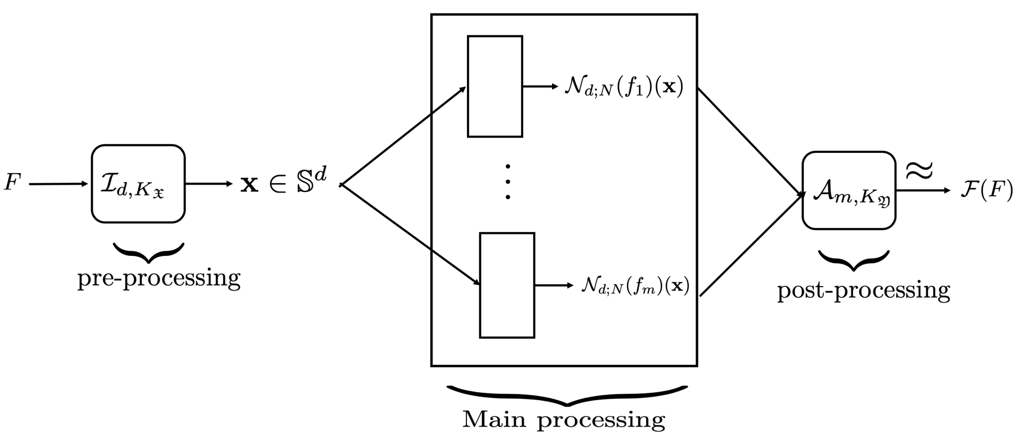
In our theory, we assume that an appropriate (if not optimal) choice of the operators ℐd,K𝔛\mathcal{I}_{d,K_{\mathfrak{X}}}, 𝒜d,K𝔛\mathcal{A}_{d,K_{\mathfrak{X}}}, ℐm,K𝔜\mathcal{I}_{m,K_{\mathfrak{Y}}}, 𝒜m,K𝔜\mathcal{A}_{m,K_{\mathfrak{Y}}} is already made based on domain knoweldge. The problem of approximating ℱ⁡(F)\mathcal{F}(F) for any F∈K𝔛F\in K_{\mathfrak{X}} is thus reduced to the problem of approximating mm functions of the form fj:ℝd→ℝf_{j}:{\mathbb{R}}^{d}\to{\mathbb{R}} so that fj​(ℐd,K𝔛​(F))f_{j}(\mathcal{I}_{d,K_{\mathfrak{X}}}(F)) is the jj-th component of ℐm,K𝔜​(ℱ⁡(𝒜d,K𝔛​(ℐd,K𝔛​(F))))\displaystyle\mathcal{I}_{m,K_{\mathfrak{Y}}}\left(\mathcal{F}(\mathcal{A}_{d,K_{\mathfrak{X}}}\left(\mathcal{I}_{d,K_{\mathfrak{X}}}(F)\right))\right). This idea is presented pictorially in Figure 1.
Refer to caption
Figure 1: Schematics for operator approximation, see text for the explaination of symbols. The output of the box labeled 𝒜m,K𝔜\mathcal{A}_{m,K_{\mathfrak{Y}}} is actually an approximation to ℱ⁡(F)\mathcal{F}(F) as indicated in (3.11).

To illustrate the error estimate in the approximation of ℱ\mathcal{F} while keeping the notation relatively simple, let us assume that ℱ\mathcal{F}, ℐd,K𝔛\mathcal{I}_{d,K_{\mathfrak{X}}}, 𝒜d,K𝔛\mathcal{A}_{d,K_{\mathfrak{X}}}, ℐm,K𝔜\mathcal{I}_{m,K_{\mathfrak{Y}}}, 𝒜m,K𝔜\mathcal{A}_{m,K_{\mathfrak{Y}}} are all Lipschitz continuous. Because of continuity and compactness, there exists a compact subset KS⊂C0​(ℝd)K_{S}\subset C_{0}({\mathbb{R}}^{d}) such that each fj∈KSf_{j}\in K_{S}. We emphasize that KSK_{S} need not consist of the possible fjf_{j}’s alone; the only requirement is that they all be in KSK_{S}. Suppose we find an approximation operator 𝔾d;N:KS→C0​(ℝd)\mathbb{G}_{d;N}:K_{S}\to C_{0}({\mathbb{R}}^{d}) depending upon NN parameters such that

supf∈KS‖f−𝔾d;N​(f)‖∞≤ϵd,N,\sup_{f\in K_{S}}\|f-\mathbb{G}_{d;N}(f)\|_{\infty}\leq\epsilon_{d,N}, (3.10)

then it is easy to deduce that

supF∈K𝔛ρ𝔜​(ℱ⁡(F),𝒜m,K𝔜CLOSE\displaystyle\sup_{F\in K_{\mathfrak{X}}}\rho_{\mathfrak{Y}}\bigg(\mathcal{F}(F),\mathcal{A}_{m,K_{\mathfrak{Y}}} OPEN({(𝔾d;N​(fj)​(ℐd,K𝔛​(F)))}))\displaystyle\big(\{\left(\mathbb{G}_{d;N}(f_{j})(\mathcal{I}_{d,K_{\mathfrak{X}}}(F))\right)\}\big)\bigg) (3.11)
≤L⁡{𝗐𝗈𝗋⁡(K𝔛,𝒜d,K𝔛,ℐd,K𝔛)+ϵd,N+𝗐𝗈𝗋⁡(K𝔜,𝒜m,K𝔜,ℐm,K𝔜)},\displaystyle\leq L\left\{\mathsf{wor}(K_{\mathfrak{X}};\mathcal{A}_{d,K_{\mathfrak{X}}},\mathcal{I}_{d,K_{\mathfrak{X}}})+\epsilon_{d,N}+\mathsf{wor}(K_{\mathfrak{Y}};\mathcal{A}_{m,K_{\mathfrak{Y}}},\mathcal{I}_{m,K_{\mathfrak{Y}}})\right\},

where LL depends upon the various Lipschitz constants involved. A crude estimate of the number of parameters in the process is d​N​mdNm.

3.3 A transformation

In (3.11), the two worst case errors come from the application domain and the choice of ℐd,K𝔛\mathcal{I}_{d,K_{\mathfrak{X}}}, 𝒜d,K𝔛\mathcal{A}_{d,K_{\mathfrak{X}}}, ℐm,K𝔜\mathcal{I}_{m,K_{\mathfrak{Y}}}, 𝒜m,K𝔜\mathcal{A}_{m,K_{\mathfrak{Y}}} In order to make the two 𝗐𝗈𝗋\mathsf{wor} expressions small, one needs to make dd, mm large. To keep ϵd,N\epsilon_{d,N} under control, one has to make NN large also. Thus, the problem involves an approximation of a large number mm of functions on a space of a large dimension dd by a class with high complexity NN. It is clear that the bottleneck is the estimation of ϵd,N\epsilon_{d,N}, so that it is critical to investigate the dependence of ϵd,N\epsilon_{d,N} on both dd and NN.

Before describing the contributions of our paper, we find it convenient to make a transformation of this problem. For integer n≥1n\geq 1, we use the notation 𝐱=(x1,⋯,xn)∈ℝn\mathbf{x}=(x_{1},\cdots,x_{n})\in{\mathbb{R}}^{n},

|𝐱|n=(∑k=1nxk2)1/2.|\mathbf{x}|_{n}=\left(\sum_{k=1}^{n}x_{k}^{2}\right)^{1/2}.

We map ℝd{\mathbb{R}}^{d} to the unit sphere:

𝕊d={𝐱∈ℝd+1:|𝐱|d+1=1},{\mathbb{S}}^{d}=\{\mathbf{x}\in{\mathbb{R}}^{d+1}:|\mathbf{x}|_{d+1}=1\},

and its upper hemisphere:

𝕊+d={𝐱∈𝕊d:xd+1>0}.{\mathbb{S}}^{d}_{+}=\{\mathbf{x}\in{\mathbb{S}}^{d}:x_{d+1}>0\}.

One of the reasons for this transformation is that the compactness of 𝕊d{\mathbb{S}}^{d} simplifies the analysis rather than using the compact open topology on ℝd{\mathbb{R}}^{d} directly. We consider the mapping π∗:ℝd→𝕊+d\pi^{*}:{\mathbb{R}}^{d}\to{\mathbb{S}}^{d}_{+} given by

π∗​(x1,⋯,xd)=(x11+|𝐱|d2,⋯,xd1+|𝐱|d2,11+|𝐱|d2).\pi^{*}(x_{1},\cdots,x_{d})=\left(\frac{x_{1}}{\sqrt{1+|\mathbf{x}|_{d}^{2}}},\cdots,\frac{x_{d}}{\sqrt{1+|\mathbf{x}|_{d}^{2}}},\frac{1}{\sqrt{1+|\mathbf{x}|_{d}^{2}}}\right). (3.12)

We note that

(π∗)−1​(u1,⋯,ud+1)=(u1ud+1,⋯,udud+1).(\pi^{*})^{-1}(u_{1},\cdots,u_{d+1})=\left(\frac{u_{1}}{u_{d+1}},\cdots,\frac{u_{d}}{u_{d+1}}\right). (3.13)

The Frobenius norms of the Jacobians d​π∗d\pi^{*} and d(π∗)−1d(\pi*)^{-1} are given by

∥dπ∗∥F2=d+(d−1)​|𝐱|d2(1+|𝐱|d2)2,∥d(π∗)−1∥F2=d−1ud+12+|(u1,⋯,ud+1)|d+12ud+12.\|d\pi^{*}\|_{F}^{2}=\frac{d+(d-1)|\mathbf{x}|_{d}^{2}}{(1+|\mathbf{x}|_{d}^{2})^{2}},\quad\|d(\pi*)^{-1}\|_{F}^{2}=\frac{d-1}{u_{d+1}^{2}}+\frac{|(u_{1},\cdots,u_{d+1})|_{d+1}^{2}}{u_{d+1}^{2}}. (3.14)

We note two consequences of (3.14).

First, it is elementary calculus to verify using (3.14) that for any compact set K⊂ℝdK\subset{\mathbb{R}}^{d}, there exist positive constants c1​(d,K)c_{1}(d,K), c2​(d,K)c_{2}(d,K) such that

c1​(d,K)​|π∗​(𝐱)−π∗​(𝐲)|d+1≤|𝐱−𝐲|d≤c2​(d,K)|π∗​(𝐱)−π∗​(𝐲)|d+1,𝐱,𝐲∈K.c_{1}(d,K)|\pi^{*}(\mathbf{x})-\pi^{*}(\mathbf{y})|_{d+1}\leq|\mathbf{x}-\mathbf{y}|_{d}\leq c_{2}(d,K)|\pi^{*}(\mathbf{x})-\pi^{*}(\mathbf{y})|_{d+1},\qquad\mathbf{x},\mathbf{y}\in K.

We note that the dependence on dd of c1​(d,K)c_{1}(d,K), c2​(d,K)c_{2}(d,K) is ∼d1/2\sim d^{1/2}.

Second, π∗\pi^{*} is a diffeomorphism from ℝd{\mathbb{R}}^{d} to 𝕊+d{\mathbb{S}}^{d}_{+}. Continuous functions on ℝd{\mathbb{R}}^{d} vanishing at infinity are mapped to continuous, even functions on 𝕊d{\mathbb{S}}^{d}, preserving smoothness. In particular, there is no loss of generality or smoothness of the functions involved if the operator ℐd;K𝔛\mathcal{I}_{d;K_{\mathfrak{X}}} takes values in 𝕊d{\mathbb{S}}^{d} rather than ℝd{\mathbb{R}}^{d}. Thus, the problem of approximating a function of ℐd;K𝔛​(F)\mathcal{I}_{d;K_{\mathfrak{X}}}(F) may be transformed into the problem of approximation of a function on 𝕊d{\mathbb{S}}^{d}.

Similar transformations from a Euclidean ball to the sphere are well known in approximation theory (e.g., [5, 43]). We have only given one example of how such a transformation can be made in general. As argued in [40], the transformation simplifies the study of neural networks with ReLU activation function by representing them as zonal function networks instead. (A zonal function network is a function of the form 𝐱↦∑k=1nak​ϕ​(𝐰k⋅𝐱)\mathbf{x}\mapsto\sum_{k=1}^{n}a_{k}\phi(\mathbf{w}_{k}\cdot\mathbf{x}), 𝐰k,𝐱∈𝕊d\mathbf{w}_{k},\mathbf{x}\in{\mathbb{S}}^{d}, ak∈ℝa_{k}\in{\mathbb{R}}.)

For approximation on the sphere, spherical polynomials are the most natural class of approximants. In several papers [37, 29, 34], we have described how spherical polynomials can be synthesized as zonal function networks with fixed weights independent of the function being approximated (target function). Our zonal function networks are linear operators on C⁡(𝕊d)C({\mathbb{S}}^{d}), and can be written as linear combination of pre-fabricated networks with coefficients given by the values of the target function at scattered data on the sphere. This feature is extremely important in our current problem where a lot of functions need to be approximated. It ensures that the networks don’t need to be trained separately for each function as is done, e.g., in [24]. Given the close connection between zonal function networks and spherical polynomials already established in our previous papers, we will focus in this paper on approximation by spherical polynomials, mainly with the objective of dealing with the trade-off mentioned at the beginning of this sub-section.

3.4 Contributions of this paper

We highlight some of the main contributions of this paper.

  1. 1.

    Our construction in the “main processing” step in Figure 1 involves pre-fabricated “networks” 𝔾d;N\mathbb{G}_{d;N} using NN parameters in each sub-box of that box, so that the entire process involves m​NmN pre-computed parameters. There is no training involved in the traditional sense. The actual computation of ℱ⁡(F)\mathcal{F}(F) then involves only mm matrix vector multiplications. Thus, the total number of parameters is (d+N)​m(d+N)m rather than d​N​MdNM.

  2. 2.

    Unlike most other papers on the subject of approximation of operators, we provide error estimates in the supremum norm rather than a Hilbert space norm, and in fact, provide pointwise estimates in both deterministic and probabilistic sense (rather than in the sense of an expected value of a loss function).

  3. 3.

    While approximation on the sphere is very well studied, the error bounds for approximation of smooth target functions typically involve unspecified constants depending upon the dimension of the sphere. The known examples where the constants can be computed explicitly involve constants that grow exponentially with the dimension (e.g., [14, 31]). Part of the problem is in the definition of the right smoothness classes. We define a smoothness class that is a natural generalization of the notion of Lipschitz continuity, and prove approximation results with constants of the form d1/6d^{1/6}. In [48], Newman and Shapiro have given bounds with constants that are independent of the dimension, but these hold only for Lipschitz continuous functions. We could not find a reference where similar bounds are achieved for functions with higher smoothness.

  4. 4.

    We achieve approximation using linear operators for which we give explicit constructions using either values of the target function at arbitrary locations on 𝕊d{\mathbb{S}}^{d} (scattered data, in contrast to designated locations such as the points at which special quadrature formulas such as Driscoll-Healy hold), or Fourier-Laplace coefficients of ff.

  5. 5.

    We prove two kinds of local approximation results.

    1. (a)

      One is that the approximation of f∈C⁡(𝕊d)f\in C({\mathbb{S}}^{d}) near a point 𝐱∈𝕊d\mathbf{x}\in{\mathbb{S}}^{d} involves only the values of ff in a small neighborhood of 𝐱\mathbf{x}. This mitigates the effect of requiring a large number of functions in K𝔛K_{\mathfrak{X}} to obtain an approximation to ℱ⁡(F)\mathcal{F}(F) even for a single function FF.

    2. (b)

      The second aspect is to construct a globally defined operator for approximation with the property that the degree of approximation at any point adjusts automatically according to the smoothness of the target function at that point.

  6. 6.

    The ideas in the paper can be extended in various ways.

    1. (a)

      Since K𝔛K_{\mathfrak{X}} is a compact set, for every ϵ>0\epsilon>0, there exists a finite cover of the set with finitely many balls of radius <ϵ<\epsilon. Denoting the centers of this ball by FℓF_{\ell}, a possibly time consuming approximation of ℱ⁡(Fℓ)\mathcal{F}(F_{\ell}) at the centers of each of these balls would give us a table so that ℱ⁡(F)\mathcal{F}(F) can be computed using a table look-up, where we find FℓF_{\ell} close to FF and return the value of ℱ⁡(Fℓ)\mathcal{F}(F_{\ell}) as an approximation to ℱ⁡(F)\mathcal{F}(F).

    2. (b)

      It is possible to iterate this paradigm somewhat trivially to the case when one wants to approximate an operator acting on the space of operators, and so on.

4 Preparatory material

In order to state our main results in Section 5, we need to describe some background on approximation on the sphere. It is necessary for our proofs also to introduce some basic concepts about Jacobi polynomials. Section 4.1 discusses some elementary facts about Jacobi polynomials. In Section 4.2, we introduce some basic facts about the sphere, including spherical polynomials and their connection with Jacobi polynomials. An essential role in our theory is played by quadrature formulas on the sphere, which are discussed in Section 4.3. The kernels and operators which are used in our constructions are described in Section 4.4.

4.1 Jacobi polynomials

A standard reference for the material here is the book [58] of Szegö. For α,β>−1\alpha,\beta>-1, x∈(−1,1)x\in(-1,1) and integer ℓ≥0\ell\geq 0, the Jacobi polynomials pℓ(α,β)p_{\ell}^{(\alpha,\beta)} are defined by the Rodrigues’ formula [58, Formulas (4.3.1), (4.3.4)]

(1−x)α​(1+x)β​pℓ(α,β)​(x)={2​ℓ+α+β+12α+β+1​Γ⁡(ℓ+1)​Γ​(ℓ+α+β+1)Γ⁡(ℓ+α+1)​Γ​(ℓ+β+1)}1/2​(−1)ℓ2ℓ​ℓ!​dℓd​xℓ​((1−x)ℓ+α​(1+x)ℓ+β).(1-x)^{\alpha}(1+x)^{\beta}p_{\ell}^{(\alpha,\beta)}(x)=\left\{\frac{2\ell+\alpha+\beta+1}{2^{\alpha+\beta+1}}\frac{\Gamma(\ell+1)\Gamma(\ell+\alpha+\beta+1)}{\Gamma(\ell+\alpha+1)\Gamma(\ell+\beta+1)}\right\}^{1/2}\frac{(-1)^{\ell}}{2^{\ell}\ell!}\frac{d^{\ell}}{dx^{\ell}}\left((1-x)^{\ell+\alpha}(1+x)^{\ell+\beta}\right). (4.1)

Each pℓ(α,β)p_{\ell}^{(\alpha,\beta)} is a polynomial of degree ℓ\ell with positive leading coefficient. We have the orthogonality relation

∫−11pℓ(α,β)​(x)​pj(α,β)​(x)​(1−x)α​(1+x)β​𝑑x=δℓ,j,\int_{-1}^{1}p_{\ell}^{(\alpha,\beta)}(x)p_{j}^{(\alpha,\beta)}(x)(1-x)^{\alpha}(1+x)^{\beta}dx=\delta_{\ell,j}, (4.2)

and

pℓ(α,β)​(1)\displaystyle p_{\ell}^{(\alpha,\beta)}(1) ={2​ℓ+α+β+12α+β+1​Γ⁡(ℓ+1)​Γ​(ℓ+α+β+1)Γ⁡(ℓ+α+1)​Γ​(ℓ+β+1)}1/2​Γ⁡(ℓ+α+1)Γ⁡(α+1)​Γ​(ℓ+1)\displaystyle=\left\{\frac{2\ell+\alpha+\beta+1}{2^{\alpha+\beta+1}}\frac{\Gamma(\ell+1)\Gamma(\ell+\alpha+\beta+1)}{\Gamma(\ell+\alpha+1)\Gamma(\ell+\beta+1)}\right\}^{1/2}\frac{\Gamma(\ell+\alpha+1)}{\Gamma(\alpha+1)\Gamma(\ell+1)} (4.3)
={2​ℓ+α+β+12α+β+1​Γ⁡(ℓ+α+1)​Γ​(ℓ+α+β+1)Γ⁡(ℓ+1)​Γ​(ℓ+β+1)}1/2​1Γ⁡(α+1).\displaystyle=\left\{\frac{2\ell+\alpha+\beta+1}{2^{\alpha+\beta+1}}\frac{\Gamma(\ell+\alpha+1)\Gamma(\ell+\alpha+\beta+1)}{\Gamma(\ell+1)\Gamma(\ell+\beta+1)}\right\}^{1/2}\frac{1}{\Gamma(\alpha+1)}.

We have ([58, Formula (4.5.3), (4.3.4)], [31, Formula (41), (42)])

Kn(α,β)​(x)=∑ℓ=0n−1pℓ(α,β)​(1)​pℓ(α,β)​(x)=2​α+22​n+α+β​pn−1(α+1,β)​(1)​pn−1(α+1,β)​(x),K_{n}^{(\alpha,\beta)}(x)=\sum_{\ell=0}^{n-1}p_{\ell}^{(\alpha,\beta)}(1)p_{\ell}^{(\alpha,\beta)}(x)=\frac{2\alpha+2}{2n+\alpha+\beta}p_{n-1}^{(\alpha+1,\beta)}(1)p_{n-1}^{(\alpha+1,\beta)}(x), (4.4)

and

Kn(α,β)​(1)=∑ℓ=0n−1pℓ(α,β)​(1)2=12α+β+1​Γ​(α+1)​Γ​(α+2)​Γ⁡(n+α+1)​Γ​(n+α+β+1)Γ⁡(n)​Γ​(n+β)K_{n}^{(\alpha,\beta)}(1)=\sum_{\ell=0}^{n-1}p_{\ell}^{(\alpha,\beta)}(1)^{2}=\frac{1}{2^{\alpha+\beta+1}\Gamma(\alpha+1)\Gamma(\alpha+2)}\frac{\Gamma(n+\alpha+1)\Gamma(n+\alpha+\beta+1)}{\Gamma(n)\Gamma(n+\beta)} (4.5)

Clearly, for any polynomial PP of degree <n<n,

∫−11P⁡(x)​Kn(α,β)​(x)​(1−x)α​(1+x)β​𝑑x=P⁡(1),\int_{-1}^{1}P(x)K_{n}^{(\alpha,\beta)}(x)(1-x)^{\alpha}(1+x)^{\beta}dx=P(1), (4.6)

and in particular,

∫−11(Kn(α,β)​(x))2​(1−x)α​(1+x)β​𝑑x=Kn(α,β)​(1).\int_{-1}^{1}\left(K_{n}^{(\alpha,\beta)}(x)\right)^{2}(1-x)^{\alpha}(1+x)^{\beta}dx=K_{n}^{(\alpha,\beta)}(1). (4.7)

4.2 Spherical polynomials

Most of the following information is based on [45], [57, Section IV.2], and [1, Chapter XI], although we use a different notation. Let d≥1d\geq 1 be an integer, 𝕊d{\mathbb{S}}^{d} denote the unit sphere

𝕊d={𝐱=(x1,⋯,xd+1):|𝐱|d+12=x12+⋯+xd+12=1}.{\mathbb{S}}^{d}=\{\mathbf{x}=(x_{1},\cdots,x_{d+1}):|\mathbf{x}|_{d+1}^{2}=x_{1}^{2}+\cdots+x_{d+1}^{2}=1\}. (4.8)

For δ∈(0,2]\delta\in(0,2], let

𝔹⁡(𝐱,δ)={𝐲∈𝕊d:|𝐱−𝐲|d+1≤δ}.{\mathbb{B}}(\mathbf{x},\delta)=\{\mathbf{y}\in{\mathbb{S}}^{d}:|\mathbf{x}-\mathbf{y}|_{d+1}\leq\delta\}. (4.9)

Let μd∗\mu_{d}^{*} be the Riemannian volume measure on 𝕊d{\mathbb{S}}^{d}, normalized so that μd∗​(𝕊d)=1\mu_{d}^{*}({\mathbb{S}}^{d})=1. We note that the volume of 𝕊d{\mathbb{S}}^{d} itself is given by

ωd=2​π(d+1)/2Γ⁡((d+1)/2)=π​Γ​(d/2)Γ⁡((d+1)/2)​ωd−1={ωd−1​∫−11(1−x2)d/2−1​dx,if d≥2,2​π,if d=1,\omega_{d}=\frac{2\pi^{(d+1)/2}}{\Gamma((d+1)/2)}=\frac{\sqrt{\pi}\Gamma(d/2)}{\Gamma((d+1)/2)}\omega_{d-1}=\begin{cases}\displaystyle\omega_{d-1}\int_{-1}^{1}(1-x^{2})^{d/2-1}dx,&\mbox{if $d\geq 2$,}\\[4.30554pt] 2\pi,&\mbox{if $d=1$,}\end{cases} (4.10)

and the measure μd∗\mu_{d}^{*} is defined recursively by

d​μd∗={ωd−1ωd​d​μd−1∗​(𝐱′)​sind−1⁡θ​d​θ,𝐱=(𝐱′​sin⁡θ,cos⁡θ)∈𝕊d,𝐱′∈𝕊d−1, if d≥2,12​π​d​θ,𝐱=(sin⁡θ,cos⁡θ)∈𝕊1, if d=1.d\mu_{d}^{*}=\begin{cases}\displaystyle\frac{\omega_{d-1}}{\omega_{d}}d\mu_{d-1}^{*}(\mathbf{x}^{\prime})\sin^{d-1}\theta d\theta,\qquad\mathbf{x}=(\mathbf{x}^{\prime}\sin\theta,\cos\theta)\in{\mathbb{S}}^{d},\quad\mathbf{x}^{\prime}\in{\mathbb{S}}^{d-1},&\mbox{ if $d\geq 2$},\\[6.45831pt] \displaystyle\frac{1}{2\pi}d\theta,\qquad\mathbf{x}=(\sin\theta,\cos\theta)\in{\mathbb{S}}^{1},&\mbox{ if $d=1$}.\end{cases} (4.11)

The measure μd∗\mu_{d}^{*} is rotation invariant. Therefore, it is easy to verify that if f:[−1,1]→ℝf:[-1,1]\to{\mathbb{R}} and t↦f⁡(t)​(1−t2)d/2−1t\mapsto f(t)(1-t^{2})^{d/2-1} is integrable with respect to the Lebesgue measure on [−1,1][-1,1], then

∫𝕊df⁡(𝐱⋅𝐲)​d​μd∗​(𝐲)=ωd−1ωd​∫−11f⁡(t)​(1−t2)d/2−1​(t)​𝑑t,𝐱∈𝕊d.\int_{{\mathbb{S}}^{d}}f(\mathbf{x}\cdot\mathbf{y})d\mu_{d}^{*}(\mathbf{y})=\frac{\omega_{d-1}}{\omega_{d}}\int_{-1}^{1}f(t)(1-t^{2})^{d/2-1}(t)dt,\qquad\mathbf{x}\in{\mathbb{S}}^{d}. (4.12)

For a fixed integer ℓ≥0\ell\geq 0, the restriction to 𝕊d{\mathbb{S}}^{d} of a homogeneous harmonic polynomial of exact degree ℓ\ell is called a spherical harmonic of degree ℓ\ell. The class of all spherical harmonics of degree ℓ\ell will be denoted by ℍℓd{\mathbb{H}}^{d}_{\ell}. The spaces ℍℓd{\mathbb{H}}^{d}_{\ell} are mutually orthogonal relative to the inner product of L2​(μd∗)L^{2}(\mu_{d}^{*}). An orthonormal basis for ℍℓd{\mathbb{H}}^{d}_{\ell} is {Yℓ,k}k=1,⋯,𝖽𝗂𝗆⁡(ℍℓd)\{Y_{\ell,k}\}_{k=1,\cdots,\mathsf{dim}({\mathbb{H}}^{d}_{\ell})}.

One has the well-known addition formula [45] and [1, Chapter XI, Theorem 4] connecting Yℓ,kY_{\ell,k}’s with Jacobi polynomials defined in (4.1):

∑k=1𝖽𝗂𝗆⁡(ℍℓd)Yℓ,k(𝐱)Yℓ,k​(𝐲)¯=ωdωd−1pℓ(d/2−1,d/2−1)(1)pℓ(d/2−1,d/2−1)(𝐱⋅𝐲),ℓ=0,1,⋯.\sum_{k=1}^{\mathsf{dim}({\mathbb{H}}^{d}_{\ell})}Y_{\ell,k}(\mathbf{x})\overline{Y_{\ell,k}(\mathbf{y})}=\frac{\omega_{d}}{\omega_{d-1}}p_{\ell}^{(d/2-1,d/2-1)}(1)p_{\ell}^{(d/2-1,d/2-1)}(\mathbf{x}\cdot\mathbf{y}),\qquad\ell=0,1,\cdots. (4.13)

For n≥0n\geq 0, we denote by Πnd\Pi_{n}^{d} the set of restrictions to 𝕊d{\mathbb{S}}^{d} of all algebraic polynomials of degree <n<n. In this definition, we allow nn to be a non-integer, so as to be able to write, for example, Πn/2d\Pi_{n/2}^{d} rather than the more cumbersome Π⌊n/2⌋d\Pi_{\lfloor n/2\rfloor}^{d}. For integers n,ℓ,d≥1n,\ell,d\geq 1, we have

𝖽𝗂𝗆⁡(Πnd)={(2​n+d−2)​Γ⁡(n+d−1)Γ⁡(n)​Γ​(d+1) if n≥2,1, if n=1,𝖽𝗂𝗆⁡(ℍℓd)={𝖽𝗂𝗆⁡(Πℓd−1) if d≥2,2 if d=1.\mathsf{dim}(\Pi_{n}^{d})=\begin{cases}\displaystyle(2n+d-2)\frac{\Gamma(n+d-1)}{\Gamma(n)\Gamma(d+1)}&\mbox{ if $n\geq 2$},\\[4.30554pt] 1,&\mbox{ if $n=1$,}\end{cases}\qquad\mathsf{dim}({\mathbb{H}}^{d}_{\ell})=\begin{cases}\mathsf{dim}(\Pi_{\ell}^{d-1})&\mbox{ if $d\geq 2$},\\[4.30554pt] 2&\mbox{ if $d=1$.}\end{cases} (4.14)

In view of (4.13), the reproducing kernel Kd;nK_{d;n} for Πnd\Pi_{n}^{d} is defined using Jacobi polynomials by

Kd;n​(x)=ωdωd−1​Kn(d/2−1,d/2−1)​(x)=2​π​Γ​((d+2)/2)Γ⁡((d+1)/2)​(2​n+d−2)​pn−1(d/2,d/2−1)​(1)​pn−1(d/2,d/2−1)​(x),x∈[−1,1].K_{d;n}(x)=\frac{\omega_{d}}{\omega_{d-1}}K_{n}^{(d/2-1,d/2-1)}(x)=\frac{2\sqrt{\pi}\Gamma((d+2)/2)}{\Gamma((d+1)/2)(2n+d-2)}p_{n-1}^{(d/2,d/2-1)}(1)p_{n-1}^{(d/2,d/2-1)}(x),\qquad x\in[-1,1]. (4.15)

Thus, we have the reproduction formula

P⁡(𝐱)=∫𝕊dP⁡(𝐲)​Kd;n​(𝐱⋅𝐲)​d​μd∗​(𝐲),P∈Πnd.P(\mathbf{x})=\int_{{\mathbb{S}}^{d}}P(\mathbf{y})K_{d;n}(\mathbf{x}\cdot\mathbf{y})d\mu_{d}^{*}(\mathbf{y}),\qquad P\in\Pi_{n}^{d}. (4.16)

Using (4.16) with Kd;n​(𝐱⋅𝐲)K_{d;n}(\mathbf{x}\cdot\mathbf{y}) in place of PP, and using (4.13), we deduce that

𝖽𝗂𝗆⁡(Πnd)=Kd;n​(1)=∫𝕊dKd;n​(𝐱⋅𝐲)2​d​μd∗​(𝐲),𝐱∈𝕊d.\mathsf{dim}(\Pi_{n}^{d})=K_{d;n}(1)=\int_{{\mathbb{S}}^{d}}K_{d;n}(\mathbf{x}\cdot\mathbf{y})^{2}d\mu_{d}^{*}(\mathbf{y}),\qquad\mathbf{x}\in{\mathbb{S}}^{d}. (4.17)

4.3 Quadrature formula

Definition 4.1

Let n≥1n\geq 1. A measure ν\nu on 𝕊d{\mathbb{S}}^{d} is called a quadrature measure of order nn if for every P∈ΠndP\in\Pi_{n}^{d},

∫𝕊dP​𝑑ν=∫𝕊dP​d​μ∗.\int_{{\mathbb{S}}^{d}}Pd\nu=\int_{{\mathbb{S}}^{d}}Pd\mu^{*}. (4.18)

A measure ν\nu is called a Marcinkiewicz-Zygmund measure of order nn (abbreviated by ν∈𝖬𝖹⁡(d,n)\nu\in\mathsf{MZ}(d;n)) if for every P∈Πn/2dP\in\Pi_{n/2}^{d}:

∫𝕊d|P|2​d​|ν|≤c​∫𝕊d|P|2​d​μ∗,\int_{{\mathbb{S}}^{d}}|P|^{2}d|\nu|\leq c\int_{{\mathbb{S}}^{d}}|P|^{2}d\mu^{*}, (4.19)

for some positive constant cc. The infimum of all such constants will be denoted by ‖|ν|‖d;n|\!|\!|\nu|\!|\!|_{d;n}. A measure ν\nu is called a Marcinkiewicz-Zygmund quadrature measure of order nn (abbreviated by ν∈𝖬𝖹𝖰⁡(d,n)\nu\in\mathsf{MZQ}(d;n)) if both (4.18) and (4.19) hold for every P∈ΠndP\in\Pi_{n}^{d}.

Remark 4.1

This definition is essentially a special case of the definition given in Section 6.1. In [12], we have proved that the condition (4.19) is equivalent to the same condition with the L2L^{2} norm replaced by the L1L^{1} norm. However, the constants there depend upon the dimension of the manifold (sphere in this context). The use of L2L^{2} norm, and requiring (4.19) to hold for Πn/2\Pi_{n/2} instead of Πn\Pi_{n} in the definition allows us to use positive quadrature formulas such as the one described in Theorem 4.1 below directly. ■\blacksquare

Remark 4.2

It is clear that if n<mn<m then a quadrature measure (respectively, Marcinkiewicz-Zygmund measure, respectively, Marcinkiewicz-Zygmund quadrature measure) of order mm is also a quadrature measure (respectively, Marcinkiewicz-Zygmund measure, respectively, Marcinkiewicz-Zygmund quadrature measure) of order nn, and ‖|ν|‖d;n≤‖|ν|‖d;m|\!|\!|\nu|\!|\!|_{d;n}\leq|\!|\!|\nu|\!|\!|_{d;m}. ■\blacksquare

Remark 4.3

In [38, 12], we have proved if 𝒞⊂𝕊d{\mathcal{C}}\subset{\mathbb{S}}^{d} is any finite set, there exist constant c1,c2>0c_{1},c_{2}>0 depending on dd with the following property: if

sup𝐱∈𝕊dmin𝐲∈𝒞⁡|𝐱−𝐲|≤c1/n,\sup_{\mathbf{x}\in{\mathbb{S}}^{d}}\min_{\mathbf{y}\in{\mathcal{C}}}|\mathbf{x}-\mathbf{y}|\leq c_{1}/n,

then there exists ν∈𝖬𝖹𝖰⁡(d,n)\nu\in\mathsf{MZQ}(d;n) such that 𝗌𝗎𝗉𝗉⁡(ν)\mathsf{supp}(\nu) is a subset of 𝒞{\mathcal{C}} containing at most c2​𝖽𝗂𝗆​(Πnd)c_{2}\mathsf{dim}(\Pi_{n}^{d}) points. Existence of a positive measure ν∈𝖬𝖹𝖰⁡(d,n)\nu\in\mathsf{MZQ}(d;n) is also proved in the same papers under the same conditions except for a smaller value of c1c_{1}. In [33], we have estimated the cardinality of a random sample 𝒞{\mathcal{C}} that allows the condition mentioned above to be within a logarithmic multiple of 𝖽𝗂𝗆⁡(Πnd)\mathsf{dim}(\Pi_{n}^{d}). The various constants in all these constructions depend upon dd in an unspecified manner. ■\blacksquare

Remark 4.4

It is clear that if ν\nu is a positive measure satisfying (4.18) for all P∈ΠndP\in\Pi_{n}^{d}, then it satisfies (4.19) automatically for P∈Πn/2dP\in\Pi_{n/2}^{d}, so that ν∈𝖬𝖹𝖰⁡(d,n)\nu\in\mathsf{MZQ}(d;n) with ‖|ν|‖d;n=1|\!|\!|\nu|\!|\!|_{d;n}=1. ■\blacksquare

Remark 4.5

We note the following theorem, called Tchakaloff’s theorem [51, Exercise 2.5.8, p. 100], that asserts in particular the existence of a positive quadrature formula satisfying (4.18) for all P∈ΠndP\in\Pi_{n}^{d} based on exactly 𝖽𝗂𝗆⁡(Πnd)\mathsf{dim}(\Pi_{n}^{d}) points.

Theorem 4.1

Let 𝕏\mathbb{X} be a compact topological space, {ϕj}j=0N−1\{\phi_{j}\}_{j=0}^{N-1} be continuous real valued functions on 𝕏\mathbb{X}, ϕ0≡1\phi_{0}\equiv 1, and μ∗\mu^{*} be a probability measure on 𝕏\mathbb{X} (i.e., μ∗\mu^{*} is a positive Borel measure with μ∗​(𝕏)=1\mu^{*}(\mathbb{X})=1). Then there exist NN points x1,⋯,xNx_{1},\cdots,x_{N} in 𝕏{\mathbb{X}}, and non–negative numbers w1,⋯,wNw_{1},\cdots,w_{N} such that

∑k=1Nwkϕj(xk)=∫𝕏ϕj(x)dμ∗(x),j=0,⋯,N−1.\sum_{k=1}^{N}w_{k}\phi_{j}(x_{k})=\int_{\mathbb{X}}\phi_{j}(x)d\mu^{*}(x),\qquad j=0,\cdots,N-1. (4.20)

An optimization procedure to compute the nodes and weights in this theorem is suggested in [32]. ■\blacksquare

4.4 Kernels and operators

Let r≥0r\geq 0. In Section 5, rr will be a parameter that defines the smoothness of the target function. In this paper, we will use heavily the following kernels, motivated by [14, 13, 31] :

Φ~d;n,r​(x)=Kd;(d+2)​n​(x)​pd​n(d/2+r,d/2−2)​(x)pd​n(d/2+r,d/2−2)​(1),\widetilde{\Phi}_{d;n,r}(x)=K_{d;(d+2)n}(x)\frac{p_{dn}^{(d/2+r,d/2-2)}(x)}{p_{dn}^{(d/2+r,d/2-2)}(1)}, (4.21)

and

Φd;n,r​(x)=Φ~d;n,r​(x)​(1+x2)n=Kd;(d+2)​n​(x)​pd​n(d/2+r,d/2−2)​(x)pd​n(d/2+r,d/2−2)​(1)​(1+x2)n.\Phi_{d;n,r}(x)=\widetilde{\Phi}_{d;n,r}(x)\left(\frac{1+x}{2}\right)^{n}=K_{d;(d+2)n}(x)\frac{p_{dn}^{(d/2+r,d/2-2)}(x)}{p_{dn}^{(d/2+r,d/2-2)}(1)}\left(\frac{1+x}{2}\right)^{n}. (4.22)

Corresponding to the two kernels, we define two operators as follows. If ν\nu is a measure on 𝕊d{\mathbb{S}}^{d} having bounded total variation and ff is integrable with respect to ν\nu, we define

σ~d;n,r​(ν,f)​(𝐱)=∫𝕊df⁡(𝐲)​Φ~d;n,r​(𝐱⋅𝐲)​𝑑ν​(𝐲),n>0,𝐱∈𝕊d,\widetilde{\sigma}_{d;n,r}(\nu,f)(\mathbf{x})=\int_{{\mathbb{S}}^{d}}f(\mathbf{y})\widetilde{\Phi}_{d;n,r}(\mathbf{x}\cdot\mathbf{y})d\nu(\mathbf{y}),\qquad n>0,\ \mathbf{x}\in{\mathbb{S}}^{d}, (4.23)

and

σd;n,r​(ν,f)​(𝐱)=∫𝕊df⁡(𝐲)​Φd;n,r​(𝐱⋅𝐲)​𝑑ν​(𝐲),n>0,𝐱∈𝕊d.\sigma_{d;n,r}(\nu,f)(\mathbf{x})=\int_{{\mathbb{S}}^{d}}f(\mathbf{y})\Phi_{d;n,r}(\mathbf{x}\cdot\mathbf{y})d\nu(\mathbf{y}),\qquad n>0,\ \mathbf{x}\in{\mathbb{S}}^{d}. (4.24)

The operators defined above provide good approximation in the sense which we now describe.

Constant convention

In the sequel, the notation A≲BA\lesssim B will denote A≤c​BA\leq cB for a positive constant cc that may depend upon fixed parameters under discussion, such as the smoothness parameter rr to be introduced in Section 5, but independent of dd, nn, ff, or the points on the sphere. The notation A≳BA\gtrsim B will mean B≲AB\lesssim A, and A∼BA\sim B will mean A≲B≲AA\lesssim B\lesssim A. The notation A=B+𝒪⁡(C)A=B+{\cal O}(C) will mean |A−B|≲C|A-B|\lesssim C. ■\blacksquare

For f∈C⁡(𝕊d)f\in C({\mathbb{S}}^{d}), we denote

Ed;n​(f)=minP∈Πnd⁡‖f−P‖∞.E_{d;n}(f)=\min_{P\in\Pi_{n}^{d}}\|f-P\|_{\infty}. (4.25)
Theorem 4.2

Let d≥3d\geq 3, r≥0r\geq 0, n≥2​(d+1)n\geq 2(d+1), and f∈C⁡(𝕊d)f\in C({\mathbb{S}}^{d}).
(a) If n,r>0n,r>0, P∈ΠnP\in\Pi_{n}, and ν\nu is a quadrature measure of order 2​(d+2)​n2(d+2)n, then σd;n,r​(ν,P)=P\sigma_{d;n,r}(\nu,P)=P, σ~d;n,r​(P)=P\widetilde{\sigma}_{d;n,r}(P)=P. (b) If ν∈𝖬𝖹𝖰​(d,2​(d+2)​n)\nu\in\mathsf{MZQ}(d;2(d+2)n), then

Ed;2​(d+2)​n​(f)≤‖f−σ~d;n,r​(ν,f)‖∞≲d1/6​‖|ν|‖d;2​(d+2)​n​Ed;n​(f),E_{d;2(d+2)n}(f)\leq\|f-\widetilde{\sigma}_{d;n,r}(\nu,f)\|_{\infty}\lesssim d^{1/6}|\!|\!|\nu|\!|\!|_{d;2(d+2)n}E_{d;n}(f), (4.26)

and

Ed;2​(d+2)​n​(f)≤‖f−σd;n,r​(ν,f)‖∞≲d1/6​‖|ν|‖d;2​(d+2)​n​Ed;n​(f).E_{d;2(d+2)n}(f)\leq\|f-\sigma_{d;n,r}(\nu,f)\|_{\infty}\lesssim d^{1/6}|\!|\!|\nu|\!|\!|_{d;2(d+2)n}E_{d;n}(f). (4.27)

5 Main results

In this section, we describe our main results on the degree of approximation on 𝕊d{\mathbb{S}}^{d}. We recall from Section 3.2 that each point on 𝕊d{\mathbb{S}}^{d} is potentially π∗​(ℐd,K𝔛​(F))\pi^{*}(\mathcal{I}_{d,K_{\mathfrak{X}}}(F)) (cf. (3.12)) for some F∈K𝔛F\in K_{\mathfrak{X}}. So, for example, when we discuss points in a neighborhood of 𝐱=π∗​(ℐd,K𝔛​(F))∈𝕊d\mathbf{x}=\pi^{*}(\mathcal{I}_{d,K_{\mathfrak{X}}}(F))\in{\mathbb{S}}^{d}, it is understood that the discussion refers to functions in a neighborhood of FF.

Our first theorem deals with local approximation of smooth functions. There are many definitions of smoothness of a function on the sphere (e.g., [5]). Unlike the moduli of smoothness defined in the cited book, our definition (motivated by [56, Chapter VI, Section 2.3]) is coordinate free. We find it also more natural, and it leads to the right constants in our theorem below.

We recall that a function f∈C⁡(𝕊d)f\in C({\mathbb{S}}^{d}) satisfies a Hölder condition of order r∈(0,1]r\in(0,1] if

|f⁡(𝐱)−f⁡(𝐲)|≤c⁡(f)​|𝐱−𝐲|d+1r,𝐱,𝐲∈𝕊d.|f(\mathbf{x})-f(\mathbf{y})|\leq c(f)|\mathbf{x}-\mathbf{y}|_{d+1}^{r},\qquad\mathbf{x},\mathbf{y}\in{\mathbb{S}}^{d}.

A local smoothness in this sense at 𝐱∈𝕊d\mathbf{x}\in{\mathbb{S}}^{d} would require the above estimate for all 𝐲\mathbf{y} in a neighborhood of 𝐱\mathbf{x}. Fixing 𝐱\mathbf{x} one can think of f⁡(𝐱)∈Π1df(\mathbf{x})\in\Pi_{1}^{d}. Thus, one can say that ff is locally Hölder at 𝐱\mathbf{x} if

minP∈Π1d⁡max𝐲∈𝔹⁡(𝐱,δ)​|f⁡(𝐲)−P⁡(𝐲)||𝐱−𝐲|d+1r<∞.\min_{P\in\Pi_{1}^{d}}\max_{\mathbf{y}\in\mathbb{B}(\mathbf{x},\delta)}\frac{|f(\mathbf{y})-P(\mathbf{y})|}{|\mathbf{x}-\mathbf{y}|_{d+1}^{r}}<\infty.

These considerations motivate the following Definition 5.1.

Definition 5.1

Let f∈C⁡(𝕊d)f\in C({\mathbb{S}}^{d}), r>0r>0 and 𝐱∈𝕊d\mathbf{x}\in{\mathbb{S}}^{d}. The function ff is said to be rr-smooth at 𝐱\mathbf{x} if there exists δ=δ⁡(d,f,𝐱)>0\delta=\delta(d;f,\mathbf{x})>0 such that

‖f‖d;r,𝐱:=‖f‖∞+minP∈Πrd⁡max𝐲∈𝔹⁡(𝐱,δ)​|f⁡(𝐲)−P⁡(𝐲)||𝐱−𝐲|d+1r<∞.\|f\|_{d;r,\mathbf{x}}:=\|f\|_{\infty}+\min_{P\in\Pi_{r}^{d}}\max_{\mathbf{y}\in\mathbb{B}(\mathbf{x},\delta)}\frac{|f(\mathbf{y})-P(\mathbf{y})|}{|\mathbf{x}-\mathbf{y}|_{d+1}^{r}}<\infty. (5.1)

The class of all f∈C⁡(𝕊d)f\in C({\mathbb{S}}^{d}) for which ‖f‖d;r,𝐱<∞\|f\|_{d;r,\mathbf{x}}<\infty will be denoted by Wd;r,𝐱W_{d;r,\mathbf{x}}. The class Wd;rW_{d;r} will denote the set of all f∈C⁡(𝕊d)f\in C({\mathbb{S}}^{d}) for which

‖f‖d;r=sup𝐱∈𝕊d‖f‖d;r,𝐱<∞.\|f\|_{d;r}=\sup_{\mathbf{x}\in{\mathbb{S}}^{d}}\|f\|_{d;r,\mathbf{x}}<\infty. (5.2)

We note that for f∈Wd;rf\in W_{d;r}, we may choose δ⁡(d,f)\delta(d;f) in (5.1) to be independent of 𝐱\mathbf{x}.

Remark 5.1

If rr is an integer and ff is rr-times differentiable in a neighborhood of 𝐱\mathbf{x}, then the function 𝐳↦f⁡(𝐳/|𝐳|d+1)\mathbf{z}\mapsto f(\mathbf{z}/|\mathbf{z}|_{d+1}), 𝐳∈ℝd+1\mathbf{z}\in{\mathbb{R}}^{d+1} is also rr-times differentiable in a Euclidean neighborhood of 𝐱\mathbf{x}. The restriction to 𝕊d{\mathbb{S}}^{d} of a Taylor polynomial of this function on the Euclidean neighborhood works as one of the polynomials in the definition (5.1). ■\blacksquare

Remark 5.2

In the definition of local smoothness of ff at 𝐱\mathbf{x}, it is tempting to let δ\delta be independent of 𝐱\mathbf{x} by noting (cf. Lemma 7.3) that

‖f‖d;r,𝐱≤‖f‖∞+minP∈Πr⁡maxy∈𝕊d​|f⁡(𝐲)−P⁡(𝐲)||𝐱−𝐲|d+1r≲δ𝐱−r​‖f‖d;r,𝐱.\|f\|_{d;r,\mathbf{x}}\leq\|f\|_{\infty}+\min_{P\in\Pi_{r}}\max_{y\in{\mathbb{S}}^{d}}\frac{|f(\mathbf{y})-P(\mathbf{y})|}{|\mathbf{x}-\mathbf{y}|_{d+1}^{r}}\lesssim\delta_{\mathbf{x}}^{-r}\|f\|_{d;r,\mathbf{x}}.

In Theorem 5.1, we wish to allow nn to be dependent on δ𝐱\delta_{\mathbf{x}} (in particular the smallest nn that satisfies all the conditions of that theorem). Therefore, the factor δ𝐱−r\delta_{\mathbf{x}}^{-r} may destroy the degree of approximation if we use in the definition the whole sphere rather than a ball of radius dependent on 𝐱\mathbf{x}. Moreover, we feel that our definition underlines the role of local smoothness better than using the whole sphere in this definition. ■\blacksquare

Our first theorem gives the local approximation properties of the operators for smooth functions.

Theorem 5.1

Let d≥3d\geq 3, 𝐱∈𝕊d\mathbf{x}\in{\mathbb{S}}^{d}, r=r⁡(𝐱)>0r=r(\mathbf{x})>0,and f∈Wd;r,𝐱f\in W_{d;r,\mathbf{x}}. Let n​d≥(d+r+1)2nd\geq(d+r+1)^{2}, ν∈𝖬𝖹𝖰​(d,2​(d+2)​n)\nu\in\mathsf{MZQ}(d;2(d+2)n). If nn is large enough so that

δn=16​r​log⁡nn≤δ⁡(d,f,𝐱),\delta_{n}=\sqrt{\frac{16r\log n}{n}}\leq\delta(d;f,\mathbf{x}), (5.3)

then

|f⁡(𝐱)−σd;n,r​(ν,f)​(𝐱)|≲d1/6𝖽𝗂𝗆​(Π2​(2+d)​nd)r/d​‖f‖Wd;r,𝐱​‖|ν|‖d;2​(d+2)​n.|f(\mathbf{x})-\sigma_{d;n,r}(\nu,f)(\mathbf{x})|\lesssim\frac{d^{1/6}}{\mathsf{dim}(\Pi_{2(2+d)n}^{d})^{r/d}}\|f\|_{W_{d;r,\mathbf{x}}}|\!|\!|\nu|\!|\!|_{d;2(d+2)n}. (5.4)

Moreover,

|f⁡(𝐱)−∫𝔹⁡(𝐱,δn)Φd;n,r​(𝐱⋅𝐲)​f​(𝐲)​𝑑ν​(𝐲)|≲d1/6𝖽𝗂𝗆​(Π2​(d+2)​nd)r/d​‖f‖Wd;r,𝐱​‖|ν|‖d;2​(d+2)​n.\left|f(\mathbf{x})-\int_{{\mathbb{B}}(\mathbf{x},\delta_{n})}\Phi_{d;n,r}(\mathbf{x}\cdot\mathbf{y})f(\mathbf{y})d\nu(\mathbf{y})\right|\lesssim\frac{d^{1/6}}{\mathsf{dim}(\Pi_{2(d+2)n}^{d})^{r/d}}\|f\|_{W_{d;r,\mathbf{x}}}|\!|\!|\nu|\!|\!|_{d;2(d+2)n}. (5.5)

All the constants involved in ≲\lesssim depend only upon r⁡(𝐱)r(\mathbf{x}) but are otherwise independent of ff, 𝐱\mathbf{x}, nn, and dd.

Remark 5.3

The estimate (5.5) shows that for any 𝐱\mathbf{x}, the approximation of f⁡(𝐱)f(\mathbf{x}) is accomplished using only values of ff in a small neighborhood of 𝐱\mathbf{x}. In the case when f∈Wd;r⁡(𝐱),𝐱f\in W_{d;r(\mathbf{x}),\mathbf{x}} for every 𝐱∈𝕊d\mathbf{x}\in{\mathbb{S}}^{d} for some r⁡(𝐱)>0r(\mathbf{x})>0, then the quantity δ⁡(d,f,𝐱)\delta(d;f,\mathbf{x}) may be chosen independent of 𝐱\mathbf{x}. The estimate (5.4) then shows that at each point 𝐱∈𝕊d\mathbf{x}\in{\mathbb{S}}^{d}, the error |f⁡(𝐱)−σd;n,r​(ν,f)​(𝐱)||f(\mathbf{x})-\sigma_{d;n,r}(\nu,f)(\mathbf{x})| adjusts automatically to the smoothness of ff at 𝐱\mathbf{x}, even though the operator is defined in a global manner without requiring any smoothness on ff at all. ■\blacksquare

Remark 5.4

In the statement of Theorem 5.1, the operator seems to depend upon the smoothness of ff near 𝐱\mathbf{x}. It will be clear from the proof that one does not need to know this smoothness beforehand; any rr greater than the actual smoothness will work. We chose to write the theorem in this way to avoid unnecessarily complicated notation that does not add much insight. ■\blacksquare

The following theorem is a global version of Theorem 5.1.

Theorem 5.2

Let d≥3d\geq 3, n≥2​(d+1)n\geq 2(d+1), and f∈C⁡(𝕊d)f\in C({\mathbb{S}}^{d}). If r>0r>0, f∈Wd;rf\in W_{d;r}, and nn is large enough so that d​n≥(d+r+1)2dn\geq(d+r+1)^{2} and(5.3) is satisfied with δ⁡(d,f)\delta(d;f) in place of δ⁡(d,f,𝐱)\delta(d;f,\mathbf{x}), then

Ed;2​(d+2)​n​(f)≲d1/6𝖽𝗂𝗆​(Π2​(d+2)​nd)r/d​‖f‖Wd;r.E_{d;2(d+2)n}(f)\lesssim\frac{d^{1/6}}{\mathsf{dim}(\Pi_{2(d+2)n}^{d})^{r/d}}\|f\|_{W_{d;r}}. (5.6)
Remark 5.5

Theorem 4.1 shows the existence of a positive measure ν∈𝖬𝖹𝖰​(d,2​(d+2)​n)\nu\in\mathsf{MZQ}(d;2(d+2)n) supported on exactly 𝖽𝗂𝗆⁡(Π2​(d+2)​nd)\mathsf{dim}(\Pi_{2(d+2)n}^{d}) points. Theorems 4.2 and 5.2 show that the operator σ~d;n,r\widetilde{\sigma}_{d;n,r} (and also σd;n,r\sigma_{d;n,r}) provide optimal approximation in the sense of nonlinear widths based on the minimal number of samples of the target function. ■\blacksquare

Next, we discuss approximation of analytic functions. The following definition is motivated by a theorem of Siciak [54] regarding approximation of functions on a unit cube which are analytic in a so-called polyellipse.

Definition 5.2

Let f∈C⁡(𝕊d)f\in C({\mathbb{S}}^{d}), 𝐱∈𝕊d\mathbf{x}\in{\mathbb{S}}^{d}, ρ>0\rho>0. The function ff is said to be ρ\rho-analytic at xx if there is exists δ=δ⁡(d,f,𝐱)>0\delta=\delta(d;f,\mathbf{x})>0 such that

‖f‖Ad;ρ,𝐱=‖f‖∞+supn≥0{exp⁡(ρ​n)​minP∈Πnd​‖f−P‖∞,𝔹⁡(𝐱,δ)}<∞.\|f\|_{A_{d;\rho,\mathbf{x}}}=\|f\|_{\infty}+\sup_{n\geq 0}\left\{\exp\left(\rho n\right)\min_{P\in\Pi_{n}^{d}}\|f-P\|_{\infty,{\mathbb{B}}(\mathbf{x},\delta)}\right\}<\infty. (5.7)

The class of all ff for which ‖f‖Ad;ρ,𝐱<∞\|f\|_{A_{d;\rho,\mathbf{x}}}<\infty will be denoted by Ad;ρ,𝐱A_{d;\rho,\mathbf{x}}. The class Ad;ρA_{d;\rho} will denote the set of all f∈C⁡(𝕊d)f\in C({\mathbb{S}}^{d}) for which

‖f‖Ad;ρ=‖f‖∞+supn>0{exp⁡(ρ​n)​Ed;n​(f)}<∞.\|f\|_{A_{d;\rho}}=\|f\|_{\infty}+\sup_{n>0}\left\{\exp\left(\rho n\right)E_{d;n}(f)\right\}<\infty. (5.8)

We note that if f∈Ad;ρf\in A_{d;\rho} then we may choose δ⁡(d,f,𝐱)\delta(d;f,\mathbf{x}) in (5.7) to be independent of 𝐱\mathbf{x}.

The following theorem describes the analogue of Theorem 5.1 for locally analytic functions. The global version is immediate from Theorem 4.2 and the definitions.

Theorem 5.3

Let d≥3d\geq 3, r≥0r\geq 0, n​d≥(d+r+1)2nd\geq(d+r+1)^{2}, ν∈𝖬𝖹𝖰​(d,2​(d+2)​n)\nu\in\mathsf{MZQ}(d;2(d+2)n). If 𝐱∈𝕊d\mathbf{x}\in{\mathbb{S}}^{d}, f∈Ad;ρ,𝐱f\in A_{d;\rho,\mathbf{x}}, and δ=δ⁡(d,f,𝐱)\delta=\delta(d;f,\mathbf{x}) be as in Definition 5.2. Then

|f⁡(𝐱)−σd;n,r​(ν,f)​(𝐱)|≲d1/6​exp⁡(−min⁡(ρ,δ2/4−2​log⁡(4/δ))​n)​‖f‖Ad;ρ,𝐱|‖ν‖|2​(d+2)​n,|f(\mathbf{x})-\sigma_{d;n,r}(\nu,f)(\mathbf{x})|\lesssim d^{1/6}\exp\left(-\min(\rho,\delta^{2}/4-2\log(4/\delta))n\right)\|f\|_{A_{d;\rho,\mathbf{x}}}|\!|\!|\nu|\!|\!|_{2(d+2)n}, (5.9)

and

|f⁡(𝐱)−∫𝔹⁡(𝐱,δ⁡(d,f,𝐱))Φd;n,r​(𝐱⋅𝐲)​f​(𝐲)​d​νn​(𝐲)|≲d1/6​exp⁡(−min⁡(ρ,δ2/4−2​log⁡(4/δ))​n)​‖f‖Ad;ρ,𝐱|‖ν‖|2​(d+2)​n.\left|f(\mathbf{x})-\int_{{\mathbb{B}}(\mathbf{x},\delta(d;f,\mathbf{x}))}\Phi_{d;n,r}(\mathbf{x}\cdot\mathbf{y})f(\mathbf{y})d\nu_{n}(\mathbf{y})\right|\lesssim d^{1/6}\exp\left(-\min(\rho,\delta^{2}/4-2\log(4/\delta))n\right)\|f\|_{A_{d;\rho,\mathbf{x}}}|\!|\!|\nu|\!|\!|_{2(d+2)n}. (5.10)

In applications to uncertainty quantification, the samples of the input functions FF (which correspond to the points on 𝕊d{\mathbb{S}}^{d} at which the target function ff is sampled) are taken from a probability distribution. Our next theorem describes the approximation properties in this set up. We consider only global approximation of smooth functions. A result for approximation of analytic functions can be proved similarly. The local approximation would involve two options. One can assume random samples from a distribution supported on a neighborhood of the point at which local approximation is considered. This case is covered by taking the function f0f_{0} in the following theorem to be supported on this neighborhood. The other option is to take the random sample on the entire sphere, but use only those which lie in a small neighborhood of the point in question. This would involve the use of multiplicative Chernoff bounds. This line of work will take us too far away from the main theme of this paper.

Theorem 5.4

Let r>0r>0, d≥3d\geq 3, ϵ>0\epsilon>0. Let M≥2M\geq 2, and 𝒞={𝐲1,⋯,𝐲M}⊂𝕊d{\mathcal{C}}=\{\mathbf{y}_{1},\cdots,\mathbf{y}_{M}\}\subset{\mathbb{S}}^{d} be random samples drawn from a probability distribution d​τ=f0​d​μd∗d\tau=f_{0}d\mu_{d}^{*} for some f0∈C⁡(𝕊d)f_{0}\in C({\mathbb{S}}^{d}). Let f∈C⁡(𝕊d)f\in C({\mathbb{S}}^{d}), r>0r>0, f0​f∈Wd;rf_{0}f\in W_{d;r}, nn be large enough to satisfy the conditions of Theorem 5.2(b). We define

σ^d;n,r​(𝒞,f)​(x)=1M​∑j=1Mf⁡(𝐲j)​Φd;n,r​(𝐱⋅𝐲j),𝐱∈𝕊d.\widehat{\sigma}_{d;n,r}({\mathcal{C}},f)(x)=\frac{1}{M}\sum_{j=1}^{M}f(\mathbf{y}_{j})\Phi_{d;n,r}(\mathbf{x}\cdot\mathbf{y}_{j}),\qquad\mathbf{x}\in{\mathbb{S}}^{d}. (5.11)

With Dn=𝖽𝗂𝗆⁡(Π2​(d+2)​nd)=Kd;2​(d+2)​n​(1)D_{n}=\mathsf{dim}(\Pi_{2(d+2)n}^{d})=K_{d;2(d+2)n}(1), if

M≳2−dd−1/3‖f‖∞‖f0​f‖∞Dn(2​r+d)/d(logDn+(d+1)logd+dlog(16e/π)+log(1/ϵ)),M\gtrsim 2^{-d}d^{-1/3}\frac{\|f\|_{\infty}}{\|f_{0}f\|_{\infty}}D_{n}^{(2r+d)/d}\left(\log D_{n}+(d+1)\log d+d\log(16e/\pi)+\log(1/\epsilon)\right), (5.12)

with an appropriate constant involved in the inequality, then with τ\tau-probability >1−ϵ>1-\epsilon,

‖f0​f−σ^d;n,r​(𝒞,f)‖∞≲d1/6Dnr/d​‖f0​f‖Wd;r\|f_{0}f-\widehat{\sigma}_{d;n,r}({\mathcal{C}},f)\|_{\infty}\lesssim\frac{d^{1/6}}{D_{n}^{r/d}}\|f_{0}f\|_{W_{d;r}} (5.13)

Equivalently, with

B=(2​r+d)​{log⁡d+log⁡(32​e2/π)−12​d​log⁡(d+1)},M~=(2​r+d)​2dd2/3​M,B=(2r+d)\left\{\log d+\log(32e^{2}/\pi)-\frac{1}{2d}\log(d+1)\right\},\qquad\tilde{M}=\frac{(2r+d)2^{d}}{d^{2/3}}M,

and

n∼{M~log⁡M~+B}1/(2​r+d)∼{Mlog⁡M+(2​r+d)​log⁡d}1/(2​r+d)n\sim\left\{\frac{\tilde{M}}{\log\tilde{M}+B}\right\}^{1/(2r+d)}\sim\left\{\frac{M}{\log M+(2r+d)\log d}\right\}^{1/(2r+d)} (5.14)

we have

∥f0f−σ^d;n,r(𝒞,f)∥∞≲d1/6{Mlog⁡M+(2​r+d)​log⁡d}−r/(2r+d).\|f_{0}f-\widehat{\sigma}_{d;n,r}({\mathcal{C}},f)\|_{\infty}\lesssim d^{1/6}\left\{\frac{M}{\log M+(2r+d)\log d}\right\}^{-r/(2r+d)}. (5.15)

6 An example

In this section, we illustrate how to apply the theory in order to approximate an operator ℱ:C⁡(𝕏1)→C⁡(𝕏2)\mathcal{F}:C({\mathbb{X}}_{1})\to C({\mathbb{X}}_{2}), where 𝕏1{\mathbb{X}}_{1}, 𝕏2{\mathbb{X}}_{2} are smooth compact manifolds. This requires a considerable background on the theory of function approximation on manifolds, which we summarize in Section 6.1. The details for the approximation of the operator itself are given in Section 6.2.

6.1 Background

Let 𝕏{\mathbb{X}} be a compact, smooth, orientable manifold, with the geodesic metric ρ\rho, and the Riemannian volume measure μ∗\mu^{*}, normalized to be a probability measure. Let {ϕk}\{\phi_{k}\} be the basis of L2​(μ∗)L^{2}(\mu^{*}) comprising eigenfunctions of the Laplace–Beltrami operator on 𝕏{\mathbb{X}}, orthonormal with respect to μ∗\mu^{*}, with each ϕk\phi_{k} corresponding to the eigenvalue −λk2-\lambda_{k}^{2}. We assume that ϕ0≡1\phi_{0}\equiv 1, λ0=0\lambda_{0}=0, and that λk↑∞\lambda_{k}\uparrow\infty as k→∞k\to\infty. For n>0n>0, we write Πn=𝗌𝗉𝖺𝗇⁡{ϕk:λk<n}\Pi_{n}=\mathsf{span}\{\phi_{k}:\lambda_{k}<n\}, and assume that ⋃n>0Πn\bigcup_{n>0}\Pi_{n} is dense in C⁡(𝕏)C({\mathbb{X}}). We assume further the strong product assumption: there exists A∗≥2A^{*}\geq 2 such that for any P,Q∈ΠnP,Q\in\Pi_{n}, the product P​Q∈ΠA∗​nPQ\in\Pi_{A^{*}n}. We encode all these assumptions by stating that the quintuple Ξ=(𝕏,ρ,μ∗,{ϕk},{λk})\Xi=({\mathbb{X}},\rho,\mu^{*},\{\phi_{k}\},\{\lambda_{k}\}) is a system. We will mention Ξ\Xi in the notation whenever it is necessary to prescribe the system to avoid confusion; for example, we will write Πn​(Ξ)\Pi_{n}(\Xi) for Πn\Pi_{n}, En​(Ξ,f)E_{n}(\Xi;f) for En​(f)E_{n}(f) below, etc. In this appendix, ≲,≳,∼\lesssim,\gtrsim,\sim will involve constants that depend upon the system Ξ\Xi. We note that if the dimension of 𝕏{\mathbb{X}} is qq, then 𝖽𝗂𝗆⁡(Πn)∼nq\mathsf{dim}(\Pi_{n})\sim n^{q}.

A a signed (or positive) measure ν\nu on 𝕏{\mathbb{X}} with bounded total variation is called a Marcinkiewicz-Zygmund quadrature measure of order nn (i.e., ν∈𝖬𝖹𝖰⁡(n)\nu\in\mathsf{MZQ}(n)) if both of the following conditions are satisfied for all P∈ΠA∗​nP\in\Pi_{A^{*}n}:

∫𝕏P​𝑑ν=∫𝕏P​d​μ∗,∫𝕏|P|​𝑑ν≤‖|ν|‖n​∫𝕏|P|​d​μ∗\int_{{\mathbb{X}}}Pd\nu=\int_{{\mathbb{X}}}Pd\mu^{*},\qquad\int_{{\mathbb{X}}}|P|d\nu\leq|\!|\!|\nu|\!|\!|_{n}\int_{{\mathbb{X}}}|P|d\mu^{*} (6.1)

for a (minimal) positive constant ‖|ν|‖n|\!|\!|\nu|\!|\!|_{n}. In [11, 12], we have proved that there exists a constant B>0B>0 with the following property: If 𝒞⊂𝕏{\mathcal{C}}\subset{\mathbb{X}} (generally, a finite subset) satisfies

supx∈𝕏miny∈𝒞⁡ρ⁡(x,y)≤B/n,\sup_{x\in{\mathbb{X}}}\min_{y\in{\mathcal{C}}}\rho(x,y)\leq B/n,

then there exists ν∈𝖬𝖹𝖰⁡(n)\nu\in\mathsf{MZQ}(n) with 𝗌𝗎𝗉𝗉⁡(ν)⊂𝒞\mathsf{supp}(\nu)\subset{\mathcal{C}}. When 𝒞{\mathcal{C}} is finite, we may choose |𝗌𝗎𝗉𝗉⁡(ν)|∼𝖽𝗂𝗆⁡(ΠA∗​n)∼nq|\mathsf{supp}(\nu)|\sim\mathsf{dim}(\Pi_{A^{*}n})\sim n^{q}.

For f∈C⁡(𝕏)f\in C({\mathbb{X}}), we write

En​(f)=minP∈Πn⁡‖f−P‖∞;𝕏.E_{n}(f)=\min_{P\in\Pi_{n}}\|f-P\|_{\infty;{\mathbb{X}}}.

If ν\nu is a signed (or positive) measure on 𝕏j{\mathbb{X}}_{j} with bounded total variation, we define

f^​(ν,k)=∫𝕏f​ϕk​𝑑ν.\hat{f}(\nu,k)=\int_{{\mathbb{X}}}f\phi_{k}d\nu.

If f∈C⁡(𝕏)f\in C({\mathbb{X}}), and r>0r>0, we say that f∈𝕎rf\in\mathbb{W}_{r} if there exists 𝒟r​(f)∈C​(𝕏)\mathcal{D}_{r}(f)\in C({\mathbb{X}}) such that 𝒟r​(f)^​(μ∗,k)=λkr​f^​(μ∗,k)\widehat{\mathcal{D}_{r}(f)}(\mu^{*},k)=\lambda_{k}^{r}\hat{f}(\mu^{*},k), k∈ℕ0k\in\mathbb{N}_{0}, and write

‖f‖Wr=‖f‖∞,𝕏+‖𝒟r​(f)‖∞,𝕏.\|f\|_{W_{r}}=\|f\|_{\infty,{\mathbb{X}}}+\|\mathcal{D}_{r}(f)\|_{\infty,{\mathbb{X}}}. (6.2)

Then the unit ball Kr={f∈Wr:‖f‖Wr≤1}K_{r}=\{f\in W_{r}:\|f\|_{W_{r}}\leq 1\} is a compact subset of C⁡(𝕏)C({\mathbb{X}}).

Let H:ℝ→[0,1]H:{\mathbb{R}}\to[0,1] be infinitely differentiable function with H⁡(t)=1H(t)=1 for 0≤t≤1/20\leq t\leq 1/2 and H⁡(t)=0H(t)=0 for t≥1t\geq 1. We define

Φn​(x,y)=∑k=0∞H⁡(λkn)​ϕk​(x)​ϕk​(y),x,y∈𝕏,\Phi_{n}(x,y)=\sum_{k=0}^{\infty}H\left(\frac{\lambda_{k}}{n}\right)\phi_{k}(x)\phi_{k}(y),\qquad x,y\in{\mathbb{X}},

and define

σn​(ν,f)=∫𝕏f⁡(y)​Φn​(x,y)​𝑑ν​(y).\sigma_{n}(\nu,f)=\int_{{\mathbb{X}}}f(y)\Phi_{n}(x,y)d\nu(y). (6.3)

We have proved in [25, 30, 10] that if ν∈𝖬𝖹𝖰⁡(A∗​n)\nu\in\mathsf{MZQ}(A^{*}n) then

∥f−σn(ν,f)∥∞,𝕏≲n−r∼(𝖽𝗂𝗆(Πn))−r/q,f∈Kr.\|f-\sigma_{n}(\nu,f)\|_{\infty,{\mathbb{X}}}\lesssim n^{-r}\sim(\mathsf{dim}(\Pi_{n}))^{-r/q},\qquad f\in K_{r}. (6.4)

Let 𝒞⊂𝕏{\mathcal{C}}\subset{\mathbb{X}} be a finite subset, and

η=minx,y∈𝒞,x≠y⁡ρ⁡(x,y).\eta=\min_{x,y\in{\mathcal{C}},x\not=y}\rho(x,y).

It can be shown (see [26, Theorem 6.1]) for a recent proof) using the localization properties of the kernels Φn\Phi_{n} proved in [25] that the following statement holds. Let 𝐯=(vx)x∈𝒞∈ℝ|𝒞|\mathbf{v}=(v_{x})_{x\in{\mathcal{C}}}\in{\mathbb{R}}^{|{\mathcal{C}}|}. For n≳η−1n\gtrsim\eta^{-1}, the following system of equations has a unique solution (bz)z∈𝒞(b_{z})_{z\in{\mathcal{C}}}:

∑z∈𝒞bz​Φn​(x,z)=vx,x∈𝒞.\sum_{z\in{\mathcal{C}}}b_{z}\Phi_{n}(x,z)=v_{x},\qquad x\in{\mathcal{C}}. (6.5)

We will denote the function x↦∑z∈𝒞bz​Φn​(x,z)x\mapsto\sum_{z\in{\mathcal{C}}}b_{z}\Phi_{n}(x,z) by F𝐯F_{\mathbf{v}}. Clearly, the function F𝐯∈WrF_{\mathbf{v}}\in W_{r} for every r>0r>0.

6.2 Approximation of the operator

We illustrate the application of our main results in the case of approximation of operators defined on functions on a manifold. In the sense of the Section 6.1, we assume two systems Ξj=(𝕏j,ρj,μj∗,{ϕk,j},{λk,j})\Xi_{j}=({\mathbb{X}}_{j},\rho_{j},\mu_{j}^{*},\{\phi_{k,j}\},\{\lambda_{k,j}\}), j=1,2j=1,2. The constants involved in ≲\lesssim, ≳\gtrsim, ∼\sim may depend upon both the systems. In this case, the operator ℱ:C⁡(𝕏1)→C⁡(𝕏2)\mathcal{F}:C({\mathbb{X}}_{1})\to C({\mathbb{X}}_{2}), and it is desired that the approximation of this operator should take place on the unit ball K𝔛K_{\mathfrak{X}} of Ws1​(Ξ1)⊂C⁡(𝕏1)W_{s_{1}}(\Xi_{1})\subset C({\mathbb{X}}_{1}). We assume that the image of K𝔛K_{\mathfrak{X}} under ℱ\mathcal{F}, denoted by 𝒦𝔜\mathcal{K}_{\mathfrak{Y}} is a (necessarily compact in C⁡(𝕏2)C({\mathbb{X}}_{2})) subset of Ws2​(Ξ2)⊂C⁡(𝕏2)W_{s_{2}}(\Xi_{2})\subset C({\mathbb{X}}_{2}). For j=1,2j=1,2, we consider finite subsets 𝒞j⊂𝕏j{\mathcal{C}}_{j}\subset{\mathbb{X}}_{j}, such that there are measures νj∈M​Z​Q​(Ξj,A∗​(Ξj)​nj)\nu_{j}\in MZQ(\Xi_{j},A^{*}(\Xi_{j})n_{j}) supported on 𝒞j{\mathcal{C}}_{j}. Necessarily |𝒞j|=mj∼njqj|{\mathcal{C}}_{j}|=m_{j}\sim n_{j}^{q_{j}}. For j=1,2j=1,2, we consider the information operators (encoders) ℐj:C⁡(𝕏j)→ℝmj\mathcal{I}_{j}:C({\mathbb{X}}_{j})\to{\mathbb{R}}^{m_{j}} given by ℐj​(f)=(f⁡(x))x∈𝒞j\mathcal{I}_{j}(f)=(f(x))_{x\in{\mathcal{C}}_{j}}, and the the corresponding reconstruction operators given by 𝒜j=σnj(Ξj;νj;∘)\mathcal{A}_{j}=\sigma_{n_{j}}(\Xi_{j};\nu_{j};\circ). Then (cf. (6.4))

∥𝒜j(ℐj(f))−f∥C⁡(𝕏j)≲mj−sj/qj∥f∥Wsj​(Ξj),f∈Wsj(Ξj),j=1,2.\|\mathcal{A}_{j}(\mathcal{I}_{j}(f))-f\|_{C({\mathbb{X}}_{j})}\lesssim m_{j}^{-s_{j}/q_{j}}\|f\|_{W_{s_{j}}(\Xi_{j})},\qquad f\in W_{s_{j}}(\Xi_{j}),\ j=1,2. (6.6)

The question of approximating ℱ⁡(F)\mathcal{F}(F) is now reduced to approximating the function from ℝm1→ℝm2{\mathbb{R}}^{m_{1}}\to{\mathbb{R}}^{m_{2}} whose value at ℐj​(F)\mathcal{I}_{j}(F) is ℐ2​(ℱ)​(F)\mathcal{I}_{2}(\mathcal{F})(F). After the transformation to the sphere, the method suggested in Section 5 now yields the degree of approximation for this function. We summarize the application of our theory in the form of an algorithm (Figure 2).

 
Pre-computation

  • •

    Find a finitely supported quadrature measure ν∈M​Z​(d,2​(d+2)​n)\nu\in MZ(d;2(d+2)n), 𝗌𝗎𝗉𝗉⁡(ν)={𝐲1,⋯,𝐲M}⊂𝕊d\mathsf{supp}(\nu)=\{\mathbf{y}_{1},\cdots,\mathbf{y}_{M}\}\subset{\mathbb{S}}^{d}, wk=ν⁡({𝐲k})w_{k}=\nu(\{\mathbf{y}_{k}\}).

  • •

    Find fk∈Ws1​(Ξ1)f_{k}\in W_{s_{1}}(\Xi_{1}) ,k=1,⋯,M,k=1,\cdots,M such that

    𝐲k=π∗​((fk​(x))x∈𝒞1).\mathbf{y}_{k}=\pi^{*}\left((f_{k}(x))_{x\in{\mathcal{C}}_{1}}\right).
  • •

    Compute

    𝐳k=(ℱ⁡(fk)​(z))z∈𝒞2,\mathbf{z}_{k}=\left(\mathcal{F}(f_{k})(z)\right)_{z\in{\mathcal{C}}_{2}},

Approximation of the operator

Given FF,

  • •

    Compute

    𝐱=π∗​((F⁡(x))x∈𝒞1).\mathbf{x}=\pi^{*}\left((F(x))_{x\in{\mathcal{C}}_{1}}\right).
  • •

    Compute

    𝐛=∑k=1Mwk​𝐳k​Φd;n,r​(𝐱⋅𝐲k).\mathbf{b}=\sum_{k=1}^{M}w_{k}\mathbf{z}_{k}\Phi_{d;n,r}(\mathbf{x}\cdot\mathbf{y}_{k}).
  • •

    Return

    𝒜2​(𝐛).\mathcal{A}_{2}(\mathbf{b}).


Figure 2: Algorithm for approximation of ℱ:C⁡(𝕏1)→C⁡(𝕏2)\mathcal{F}:C({\mathbb{X}}_{1})\to C({\mathbb{X}}_{2}).

In this section, we write G𝐲=F(π∗)−1(𝐲)G_{\mathbf{y}}=F_{(\pi*)^{-1}(\mathbf{y})} for 𝐲∈𝕊q\mathbf{y}\in{\mathbb{S}}^{q}. We may view the operator σm1;n,r(Ξ1;ν,∘)\sigma_{m_{1};n,r}(\Xi_{1};\nu,\circ) in (4.24) as a pre-fabricated network using the functions {G𝐲:𝐲∈𝗌𝗎𝗉𝗉⁡(ν1)}\{G_{\mathbf{y}}:\mathbf{y}\in\mathsf{supp}(\nu_{1})\} as training data, and f⁡(𝐲)f(\mathbf{y}) replaced by each of the components ℱ⁡(σn1​(Ξ1,ν1,G𝐲))​(z)\mathcal{F}(\sigma_{n_{1}}(\Xi_{1};\nu_{1},G_{\mathbf{y}}))(z) for 𝐲∈𝗌𝗎𝗉𝗉⁡(ν1)\mathbf{y}\in\mathsf{supp}(\nu_{1}), z∈𝒞2z\in{\mathcal{C}}_{2} in turn. The total number of parameters in this process is N​mNm, where N=𝖽𝗂𝗆⁡(Π2​(d+2)​nd)N=\mathsf{dim}(\Pi_{2(d+2)n}^{d}). All these parameters are pre-computed and fixed for approximation of ℱ⁡(F)\mathcal{F}(F) for any F∈Ws1​(Ξ1)F\in W_{s_{1}}(\Xi_{1}). After this, for any F∈Ws1​(Ξ1)F\in W_{s_{1}}(\Xi_{1}), the approximation of ℱ⁡(F)\mathcal{F}(F) involves only d​mdm further parameters. Thus, the overall complexity of main processing (cf. Figure 1) in terms of parameters, including pre-computation, is 𝒪⁡((d+N)​m){\cal O}((d+N)m) rather than 𝒪⁡(d​N​m){\cal O}(dNm). For local approximation at F∈Ws1​(Ξ1)F\in W_{s_{1}}(\Xi_{1}), we need to use only those G𝐲G_{\mathbf{y}}’s out of the pre-computed functions that are close to FF as indicated in Theorem 5.1, resulting in a further reduction of complexity.

7 Proofs

The main purpose of this section is to prove all the theorems in Section 5. As expected, a major part of the proofs is to obtain estimates on the Lebesgue constant for Φd;n,r\Phi_{d;n,r}. It is convenient to summarize some of the required calculations in the context of Jacobi polynomials in general. Accordingly, we prove in Section 7.1 some estimates on some integrals involving Jacobi polynomials. The estimates on the Lebesgue constants and some other technical estimates about spherical polynomials are proved in Section 7.2. The proofs of the theorems in Sections 4.2 and 5 are given in Section 7.3.

7.1 Estimates on Jacobi polynomials

In this sub-section only, the notation A≲BA\lesssim B will denote A≤c​BA\leq cB for an absolute positive constant, A≳BA\gtrsim B will mean B≲AB\lesssim A, and A∼BA\sim B will mean A≲B≲AA\lesssim B\lesssim A. The notation A=B+𝒪⁡(C)A=B+{\cal O}(C) will mean |A−B|≲C|A-B|\lesssim C.

The following theorem summarizes some of the important estimates we will use in this paper.

Theorem 7.1

(a) Let a≥b≥0a\geq b\geq 0, A≥B≥1A\geq B\geq 1, 0<p<∞0<p<\infty, 2​b≥p​B+p/22b\geq pB+p/2, and 2​a+2<p​A+p/22a+2<pA+p/2. Further assume that

n≳A​{2​a+2p⁡(A+1/2)−2​a−2}1/p.n\gtrsim A\left\{\frac{2a+2}{p(A+1/2)-2a-2}\right\}^{1/p}. (7.1)

We have

∫−11\displaystyle\int_{-1}^{1} |pn(A,B)​(x)pn(A,B)​(1)|p​(1−x)a​(1+x)b​d​x\displaystyle\left|\frac{p_{n}^{(A,B)}(x)}{p_{n}^{(A,B)}(1)}\right|^{p}(1-x)^{a}(1+x)^{b}dx (7.2)
≲2a+b2​a+2​{A1/62(A+B−1)/2​pn(A,B)​(1)}(2​a+2)/(A+1/2)​{2​a+2p⁡(A+1/2)−2​a−2}(2​a+2)/p⁡(A+1/2)\displaystyle\lesssim\frac{2^{a+b}}{2a+2}\left\{\frac{A^{1/6}}{2^{(A+B-1)/2}p_{n}^{(A,B)}(1)}\right\}^{(2a+2)/(A+1/2)}\left\{\frac{2a+2}{p(A+1/2)-2a-2}\right\}^{(2a+2)/p(A+1/2)}

(b) If α≥β≥2\alpha\geq\beta\geq 2, r≥s>−1r\geq s>-1, n≥(2​α+r+1)2n\geq(2\alpha+r+1)^{2}, then

∫−11\displaystyle\int_{-1}^{1} |pn(α+r+1,β−1)​(x)pn(α+r+1,β−1)​(1)|2​(1−x)s+α​(1+x)β​d​x\displaystyle\left|\frac{p_{n}^{(\alpha+r+1,\beta-1)}(x)}{p_{n}^{(\alpha+r+1,\beta-1)}(1)}\right|^{2}(1-x)^{s+\alpha}(1+x)^{\beta}dx (7.3)
≲2α+β+s​(α+r+1)1/3​Γ​(α+r+2)(4​α+4​s+4)/(2​α+2​r+3)​n−2​α−2​s−2.\displaystyle\lesssim 2^{\alpha+\beta+s}(\alpha+r+1)^{1/3}\Gamma(\alpha+r+2)^{(4\alpha+4s+4)/(2\alpha+2r+3)}n^{-2\alpha-2s-2}.

(c) If α≥β≥2\alpha\geq\beta\geq 2, r≥s>−1r\geq s>-1, n≥(2​α+r+1)2n\geq(2\alpha+r+1)^{2}, m≥(α+β)2m\geq(\alpha+\beta)^{2}, then

Km(α,β)(1)∫−11\displaystyle K_{m}^{(\alpha,\beta)}(1)\int_{-1}^{1} |pn(α+r+1,β−1)​(x)pn(α+r+1,β−1)​(1)|2​(1−x)s+α​(1+x)β​d​x\displaystyle\left|\frac{p_{n}^{(\alpha+r+1,\beta-1)}(x)}{p_{n}^{(\alpha+r+1,\beta-1)}(1)}\right|^{2}(1-x)^{s+\alpha}(1+x)^{\beta}dx (7.4)
≲e2​r−2​s​2s​(mn)2​α+2​s+2​m−2​s​Γ​(α+r+2)2Γ⁡(α+1)​Γ​(α+2)​(α+r+2)2​s−2​r−2/3.\displaystyle\lesssim e^{2r-2s}2^{s}\left(\frac{m}{n}\right)^{2\alpha+2s+2}m^{-2s}\frac{\Gamma(\alpha+r+2)^{2}}{\Gamma(\alpha+1)\Gamma(\alpha+2)}(\alpha+r+2)^{2s-2r-2/3}.

The proof of this theorem requires some preparation. We will observe a fundamental estimate on the ratio of Gamma functions in Lemma 7.1, and apply it in Corollary 7.1 to obtain some detailed asymptotics for the various quantities introduced in Section 4.1.

Lemma 7.1

For x≥y≥1x\geq y\geq 1, we have

log⁡Γ⁡(x+y)−log⁡Γ⁡(x)=y​log​x+𝒪⁡(y2x).\log\Gamma(x+y)-\log\Gamma(x)=y\log x+{\cal O}\left(\frac{y^{2}}{x}\right). (7.5)

In particular, if x≳y2x\gtrsim y^{2} then

Γ⁡(x+y)Γ⁡(x)∼xy.\frac{\Gamma(x+y)}{\Gamma(x)}\sim x^{y}. (7.6)

Proof.

The Stirling approximation ([50, Section 4.1]) states that for z≥1z\geq 1,

log⁡Γ⁡(z)=(z−1/2)​log⁡z−z+(1/2)​log⁡(2​π)=𝒪⁡(1/z).\log\Gamma(z)=(z-1/2)\log z-z+(1/2)\log(2\pi)={\cal O}(1/z). (7.7)

Hence, for x,y≥1x,y\geq 1,

log⁡Γ⁡(x+y)−log⁡Γ⁡(x)=(x+y−1/2)​log⁡(x+y)−(x−1/2)​log​x−y+𝒪⁡(1x).\log\Gamma(x+y)-\log\Gamma(x)=(x+y-1/2)\log(x+y)-(x-1/2)\log x-y+{\cal O}\left(\frac{1}{x}\right). (7.8)

Now,

(x+y−1/2)​log⁡(x+y)=(x+y−1/2)​log⁡x+x⁡(1+yx)​log⁡(1+y/x)−12​log⁡(1+y/x).(x+y-1/2)\log(x+y)=(x+y-1/2)\log x+x\left(1+\frac{y}{x}\right)\log(1+y/x)-\frac{1}{2}\log(1+y/x). (7.9)

Using Taylor’s theorem, a simple calculation shows that for x≥y≥1x\geq y\geq 1,

(1+yx)​log⁡(1+y/x)=y/x+𝒪⁡(y2x2),log⁡(1+y/x)=y/x+𝒪⁡(y2x2).\left(1+\frac{y}{x}\right)\log(1+y/x)=y/x+{\cal O}\left(\frac{y^{2}}{x^{2}}\right),\quad\log(1+y/x)=y/x+{\cal O}\left(\frac{y^{2}}{x^{2}}\right). (7.10)

So, we obtain from (7.9) that

(x+y−1/2)​log⁡(x+y)=(x+y−1/2)​log⁡x+y+𝒪⁡(y2x).(x+y-1/2)\log(x+y)=(x+y-1/2)\log x+y+{\cal O}\left(\frac{y^{2}}{x}\right).

This estimate and (7.8) lead to (7.5). ■\blacksquare

Corollary 7.1

For α≥β≥−1/2\alpha\geq\beta\geq-1/2, n≥(α+|β|)2n\geq(\alpha+|\beta|)^{2},

pn(α,β)​(1)∼nα+1/22(α+β)/2​Γ​(α+1),p_{n}^{(\alpha,\beta)}(1)\sim\frac{n^{\alpha+1/2}}{2^{(\alpha+\beta)/2}\Gamma(\alpha+1)}, (7.11)

and

Kn(α,β)​(1)∼12α+β​Γ​(α+1)​Γ​(α+2)​n2​α+2,K_{n}^{(\alpha,\beta)}(1)\sim\frac{1}{2^{\alpha+\beta}\Gamma(\alpha+1)\Gamma(\alpha+2)}n^{2\alpha+2}, (7.12)

where we note that the constants involved in ∼\sim are absolute constants, independent of nn, α\alpha, β\beta.

Proof. The estimate (7.11) (respectively, (7.12)) follows using (4.3) (repsectively, (4.5)) and Lemma 7.1. ■\blacksquare

The following proposition summarizes some inequalities for Jacobi polynomials.

Proposition 7.1

Let α≥β≥−1/2\alpha\geq\beta\geq-1/2, n≥0n\geq 0 be an integer.
(a) We have

maxx∈[−1,1]⁡|pn(α,β)​(x)|≤pn(α,β)​(1).\max_{x\in[-1,1]}|p_{n}^{(\alpha,\beta)}(x)|\leq p_{n}^{(\alpha,\beta)}(1). (7.13)

(b) If α≥β≥(1+2)/4≈0.6036\alpha\geq\beta\geq(1+\sqrt{2})/4\approx 0.6036, n≥αn\geq\alpha, then for θ∈(0,π)\theta\in(0,\pi),

|pn(α,β)(cosθ)|≤2α1/6(1−cosθ)−α/2−1/4(1+cosθ)−β/2−1/4.|p_{n}^{(\alpha,\beta)}(\cos\theta)|\leq 2\alpha^{1/6}(1-\cos\theta)^{-\alpha/2-1/4}(1+\cos\theta)^{-\beta/2-1/4}. (7.14)

Proof. Part (a) follows from [58, Theorem 7.32.1]. Part (b) follows from [17, Theorem 2]. ■\blacksquare

We are now in a position to prove Theorem 7.1.

Proof of Theorem 7.1.
Let 0<δ<π/20<\delta<\pi/2 to be chosen later. Since b≥0b\geq 0, (7.13) leads to

∫02​δ|pn(A,B)​(cos⁡θ)|p\displaystyle\int_{0}^{2\delta}|p_{n}^{(A,B)}(\cos\theta)|^{p} (1−cosθ)a(1+cosθ)bsinθdθ≤2a+b+1|pn(A,B)(1)|p∫02​δsin(θ/2)2​a+1cos(θ/2)2​b+1dθ\displaystyle(1-\cos\theta)^{a}(1+\cos\theta)^{b}\sin\theta d\theta\leq 2^{a+b+1}|p_{n}^{(A,B)}(1)|^{p}\int_{0}^{2\delta}\sin(\theta/2)^{2a+1}\cos(\theta/2)^{2b+1}d\theta (7.15)
≤2a+b+1​|pn(A,B)​(1)|p​∫02​δsin⁡(θ/2)2​a+1​cos⁡(θ/2)​dθ≲2a+b2​a+2​|pn(A,B)​(1)|p​(sin⁡δ)2​a+2.\displaystyle\leq 2^{a+b+1}|p_{n}^{(A,B)}(1)|^{p}\int_{0}^{2\delta}\sin(\theta/2)^{2a+1}\cos(\theta/2)d\theta\lesssim\frac{2^{a+b}}{2a+2}|p_{n}^{(A,B)}(1)|^{p}(\sin\delta)^{2a+2}.

In view of (7.14), and the facts that 2​b≥p​B+p/22b\geq pB+p/2, 2​a+2<p​A+p/22a+2<pA+p/2,

∫2​δπ|pn(A,B)​(cos⁡θ)|p\displaystyle\int_{2\delta}^{\pi}|p_{n}^{(A,B)}(\cos\theta)|^{p} (1−cos⁡θ)a​(1+cos⁡θ)b​sin⁡θ​𝑑θ≲2p​Ap/6​∫2​δπ(1−cos⁡θ)a−p​A/2−p/4​(1+cos⁡θ)b−p​B/2−p/4​sin⁡θ​𝑑θ\displaystyle(1-\cos\theta)^{a}(1+\cos\theta)^{b}\sin\theta d\theta\lesssim 2^{p}A^{p/6}\int_{2\delta}^{\pi}(1-\cos\theta)^{a-pA/2-p/4}(1+\cos\theta)^{b-pB/2-p/4}\sin\theta d\theta (7.16)
≲Ap/6​2a+b−p⁡(A+B−1)/2​∫2​δπ(sin⁡(θ/2))2​a+1−p​A−p/2​(cos⁡(θ/2))2​b+1−p​B−p/2​𝑑θ\displaystyle\lesssim A^{p/6}2^{a+b-p(A+B-1)/2}\int_{2\delta}^{\pi}(\sin(\theta/2))^{2a+1-pA-p/2}(\cos(\theta/2))^{2b+1-pB-p/2}d\theta
≲Ap/6​2a+b−p⁡(A+B−1)/2​∫δπ/2(sin⁡θ)2​a+1−p​A−p/2​cos⁡θ​𝑑θ\displaystyle\lesssim A^{p/6}2^{a+b-p(A+B-1)/2}\int_{\delta}^{\pi/2}(\sin\theta)^{2a+1-pA-p/2}\cos\theta d\theta
≲Ap/6​2a+b−p⁡(A+B−1)/2p​A+p/2−2​a−2​(sin⁡δ)2​a+2−p​A−p/2.\displaystyle\lesssim\frac{A^{p/6}2^{a+b-p(A+B-1)/2}}{pA+p/2-2a-2}(\sin\delta)^{2a+2-pA-p/2}.

We now choose δ\delta such that

2a+b2​a+2​|pn(A,B)​(1)|p​(sin⁡δ)2​a+2=Ap/6​2a+b−p⁡(A+B−1)/2p​A+p/2−2​a−2​(sin⁡δ)2​a+2−p​A−p/2;\frac{2^{a+b}}{2a+2}|p_{n}^{(A,B)}(1)|^{p}(\sin\delta)^{2a+2}=\frac{A^{p/6}2^{a+b-p(A+B-1)/2}}{pA+p/2-2a-2}(\sin\delta)^{2a+2-pA-p/2};

i.e.,

sin⁡δ={A1/62(A+B−1)/2​pn(A,B)​(1)}1/(A+1/2)​{2​a+2p⁡(A+1/2)−2​a−2}1/p⁡(A+1/2).\sin\delta=\left\{\frac{A^{1/6}}{2^{(A+B-1)/2}p_{n}^{(A,B)}(1)}\right\}^{1/(A+1/2)}\left\{\frac{2a+2}{p(A+1/2)-2a-2}\right\}^{1/p(A+1/2)}.

(In view of (5.14) and (7.11), it is not difficult to verify that |sin⁡δ|≤1|\sin\delta|\leq 1.) Then (7.15) and (7.16) lead to (7.2).

Taking a=α+sa=\alpha+s, b=βb=\beta, A=α+r+1A=\alpha+r+1, B=β−1B=\beta-1, and p=2p=2, (7.2) becomes

∫−11\displaystyle\int_{-1}^{1} |pn(α+r+1,β−1)​(x)pn(α+r+1,β−1)​(1)|2​(1−x)s+α​(1+x)β​d​x\displaystyle\left|\frac{p_{n}^{(\alpha+r+1,\beta-1)}(x)}{p_{n}^{(\alpha+r+1,\beta-1)}(1)}\right|^{2}(1-x)^{s+\alpha}(1+x)^{\beta}dx (7.17)
≲2α+β+s2​α+2​s+2​{(α+r+1)1/62(α+β+r−1)/2​pn(α+r+1,β−1)​(1)}(2​α+2​s+2)/(α+r+3/2)\displaystyle\lesssim\frac{2^{\alpha+\beta+s}}{2\alpha+2s+2}\left\{\frac{(\alpha+r+1)^{1/6}}{2^{(\alpha+\beta+r-1)/2}p_{n}^{(\alpha+r+1,\beta-1)}(1)}\right\}^{(2\alpha+2s+2)/(\alpha+r+3/2)}
×{2​α+2​s+22​r−2​s+1}(2​α+2​s+2)/(2​α+2​r+3)\displaystyle\times\left\{\frac{2\alpha+2s+2}{2r-2s+1}\right\}^{(2\alpha+2s+2)/(2\alpha+2r+3)}

In this proof only, let

γ=2​α+2​s+22​α+2​r+3,1−γ=2​r−2​s+12​α+2​r+3,0<γ<1.\gamma=\frac{2\alpha+2s+2}{2\alpha+2r+3},\quad 1-\gamma=\frac{2r-2s+1}{2\alpha+2r+3},\quad 0<\gamma<1. (7.18)

We have

(21/2​(α+r+1)1/6)(2​α+2​s+2)/(α+r+3/2)=(21/2​(α+r+1)1/6)2​γ≲(α+r+1)1/3,(2​r−2​s+1)−γ≤1,(2^{1/2}(\alpha+r+1)^{1/6})^{(2\alpha+2s+2)/(\alpha+r+3/2)}=(2^{1/2}(\alpha+r+1)^{1/6})^{2\gamma}\lesssim(\alpha+r+1)^{1/3},\qquad(2r-2s+1)^{-\gamma}\leq 1,

and

(2​α+2​s+2)(2​α+2​s+2)/(2​α+2​r+3)−1=(2​α+2​s+2)γ−1≲1.(2\alpha+2s+2)^{(2\alpha+2s+2)/(2\alpha+2r+3)-1}=(2\alpha+2s+2)^{\gamma-1}\lesssim 1.

Hence, using (7.11), (7.17) simplifies to (7.3).

Next, to prove part (c), we use (7.12) and (7.3) to deduce that

Km(α,β)(1)(∫−11\displaystyle K_{m}^{(\alpha,\beta)}(1)\left(\int_{-1}^{1}\right. OPEN|pn(α+r+1,β−1)​(x)pn(α+r+1,β−1)​(1)|2​(1−x)s+α​(1+x)β​d​x)2\displaystyle\left.\left|\frac{p_{n}^{(\alpha+r+1,\beta-1)}(x)}{p_{n}^{(\alpha+r+1,\beta-1)}(1)}\right|^{2}(1-x)^{s+\alpha}(1+x)^{\beta}dx\right)^{2} (7.19)
≲m2​α+22α+β​Γ​(α+1)​Γ​(α+2)​2α+β+s​(α+r+1)1/3​Γ​(α+r+2)(4​α+4​s+4)/(2​α+2​r+3)​n−2​α−2​s−2\displaystyle\lesssim\frac{m^{2\alpha+2}}{2^{\alpha+\beta}\Gamma(\alpha+1)\Gamma(\alpha+2)}2^{\alpha+\beta+s}(\alpha+r+1)^{1/3}\Gamma(\alpha+r+2)^{(4\alpha+4s+4)/(2\alpha+2r+3)}n^{-2\alpha-2s-2}
≲2s​(α+r+1)1/3​Γ​(α+r+2)2Γ⁡(α+1)​Γ​(α+2)​Γ​(α+r+2)2​γ−2​(mn)2​α+2​s+2​m−2​s.\displaystyle\lesssim 2^{s}(\alpha+r+1)^{1/3}\frac{\Gamma(\alpha+r+2)^{2}}{\Gamma(\alpha+1)\Gamma(\alpha+2)}\Gamma(\alpha+r+2)^{2\gamma-2}\left(\frac{m}{n}\right)^{2\alpha+2s+2}m^{-2s}.

Using Stirling’s approximation, we find that

(1−γ)​log⁡Γ⁡(α+r+2)\displaystyle(1-\gamma)\log\Gamma(\alpha+r+2) =2​r−2​s+12​α+2​r+3​log⁡Γ⁡(α+r+2)\displaystyle=\frac{2r-2s+1}{2\alpha+2r+3}\log\Gamma(\alpha+r+2)
=(r−s+1/2)​log⁡(α+r+2)−2​r−2​s+12​α+2​r+3​(α+r+2)+𝒪⁡(1)\displaystyle=(r-s+1/2)\log(\alpha+r+2)-\frac{2r-2s+1}{2\alpha+2r+3}(\alpha+r+2)+{\cal O}(1)
≳(r−s+1/2)​log⁡(α+r+2)−(r−s)−c\displaystyle\gtrsim(r-s+1/2)\log(\alpha+r+2)-(r-s)-c

for some absolute constant cc. Therefore,

Γ​(α+r+2)2​γ−2≲e2​r−2​s​(α+r+2)2​s−2​r−1.\Gamma(\alpha+r+2)^{2\gamma-2}\lesssim e^{2r-2s}(\alpha+r+2)^{2s-2r-1}.

The estimate (7.4) is easy to deduce using this last estimate in (7.19). ■\blacksquare

7.2 Estimates on spherical polynomials

We will use the following proposition without explicitly referring to it.

Proposition 7.2

For d≥1d\geq 1 and n≥d2n\geq d^{2}, we have

Kd;n​(1)=𝖽𝗂𝗆⁡(Πnd)∼ndΓ⁡(d+1).K_{d;n}(1)=\mathsf{dim}(\Pi_{n}^{d})\sim\frac{n^{d}}{\Gamma(d+1)}. (7.20)

We note that the constants involved in ∼\sim are independent of nn and dd.

Proof. The relation (7.20) follows by using Lemma 7.1 in (4.14). ■\blacksquare

Next, we prove the required estimates on the Lebesgue constants for the kernels Φd;n,r\Phi_{d;n,r} and Φ~d;n,r\widetilde{\Phi}_{d;n,r}. These estimates will play a crucial role in the proof of Theorem 5.1. Therefore, we formulate them as a theorem below.

Theorem 7.2

Let d≥3d\geq 3, r≥s≥0r\geq s\geq 0, n​d≥(d+r+1)2nd\geq(d+r+1)^{2}, and ν∈𝖬𝖹​(d,2​(d+2)​n)\nu\in\mathsf{MZ}(d;2(d+2)n). Then

sup𝐱∈𝕊d∫𝕊d|Φ~d;n,r​(𝐱⋅𝐲)|​(1−𝐱⋅𝐲)s/2​d​|ν|​(𝐲)\displaystyle\sup_{\mathbf{x}\in{\mathbb{S}}^{d}}\int_{{\mathbb{S}}^{d}}|\widetilde{\Phi}_{d;n,r}(\mathbf{x}\cdot\mathbf{y})|(1-\mathbf{x}\cdot\mathbf{y})^{s/2}d|\nu|(\mathbf{y}) =sup𝐱∈𝕊d∫𝕊d|Φd;n,r​(𝐱⋅𝐲)|​(1−𝐱⋅𝐲)s/2​(1+𝐱⋅𝐲2)−n​d​|ν|​(𝐲)\displaystyle=\sup_{\mathbf{x}\in{\mathbb{S}}^{d}}\int_{{\mathbb{S}}^{d}}|\Phi_{d;n,r}(\mathbf{x}\cdot\mathbf{y})|(1-\mathbf{x}\cdot\mathbf{y})^{s/2}\left(\frac{1+\mathbf{x}\cdot\mathbf{y}}{2}\right)^{-n}d|\nu|(\mathbf{y}) (7.21)
≲d1/6ns​‖|ν|‖d;2​(d+2)​n.\displaystyle\lesssim\frac{d^{1/6}}{n^{s}}|\!|\!|\nu|\!|\!|_{d;2(d+2)n}.

Proof. In this proof, we will assume the normalization that ‖|ν|‖d;2​(d+2)​n=1|\!|\!|\nu|\!|\!|_{d;2(d+2)n}=1. We also assume that s>0s>0, and d≥6d\geq 6. The case s=0s=0 is much simpler; the approximation described in (7.22) is then not necessary. The case 3≤d≤53\leq d\leq 5 does not require an elaborate book-keeping as is done here; the same ideas work in a much simpler manner. Using the direct theorem for approximation by trigonometric polynomials to approximate the function θ↦|sin⁡(θ/2)|s\theta\mapsto|\sin(\theta/2)|^{s}, we obtain an algebraic polynomial P∈ΠnP\in\Pi_{n} such that

maxx∈[−1,1]⁡|(1−x)s/2−P⁡(x)|≲n−s.\max_{x\in[-1,1]}\left|(1-x)^{s/2}-P(x)\right|\lesssim n^{-s}. (7.22)

Since ν∈𝖬𝖹​(d,2​(d+2)​n)\nu\in\mathsf{MZ}(d;2(d+2)n), we deduce using (7.22) and Schwarz inequality that

∫𝕊d\displaystyle\int_{{\mathbb{S}}^{d}} |Φ~d;n,r​(𝐱⋅𝐲)|​(1−𝐱⋅𝐲)s/2​d​|ν|​(𝐲)≲∫𝕊d|Φ~d;n,r​(𝐱⋅𝐲)||P⁡(𝐱⋅𝐲)|d​|ν|​(𝐲)+n−s​∫𝕊q|Φ~d;n,r​(𝐱⋅𝐲)|​d​|ν|​(𝐲)\displaystyle|\widetilde{\Phi}_{d;n,r}(\mathbf{x}\cdot\mathbf{y})|(1-\mathbf{x}\cdot\mathbf{y})^{s/2}d|\nu|(\mathbf{y})\lesssim\int_{{\mathbb{S}}^{d}}|\widetilde{\Phi}_{d;n,r}(\mathbf{x}\cdot\mathbf{y})||P(\mathbf{x}\cdot\mathbf{y})|d|\nu|(\mathbf{y})+n^{-s}\int_{{\mathbb{S}}^{q}}|\widetilde{\Phi}_{d;n,r}(\mathbf{x}\cdot\mathbf{y})|d|\nu|(\mathbf{y}) (7.23)
≲{∫𝕊dKd;(d+2)​n​(𝐱⋅𝐲)2​d​|ν|​(𝐲)}1/2​{∫𝕊d|pd​n(d/2+r,d/2−2)​(𝐱⋅𝐲)pd​n(d/2+r,d/2−2)​(1)|2​|P⁡(𝐱⋅𝐲)|2​d​|ν|​(𝐲)}1/2\displaystyle\lesssim\left\{\int_{{\mathbb{S}}^{d}}K_{d;(d+2)n}(\mathbf{x}\cdot\mathbf{y})^{2}d|\nu|(\mathbf{y})\right\}^{1/2}\left\{\int_{{\mathbb{S}}^{d}}\left|\frac{p_{dn}^{(d/2+r,d/2-2)}(\mathbf{x}\cdot\mathbf{y})}{p_{dn}^{(d/2+r,d/2-2)}(1)}\right|^{2}|P(\mathbf{x}\cdot\mathbf{y})|^{2}d|\nu|(\mathbf{y})\right\}^{1/2}
+n−s​{∫𝕊dKd;(d+2)​n​(𝐱⋅𝐲)2​d​|ν|​(𝐲)}1/2​{∫𝕊d|pd​n(d/2+r,d/2−2)​(𝐱⋅𝐲)pd​n(d/2+r,d/2−2)​(1)|2​d​|ν|​(𝐲)}1/2\displaystyle+n^{-s}\left\{\int_{{\mathbb{S}}^{d}}K_{d;(d+2)n}(\mathbf{x}\cdot\mathbf{y})^{2}d|\nu|(\mathbf{y})\right\}^{1/2}\left\{\int_{{\mathbb{S}}^{d}}\left|\frac{p_{dn}^{(d/2+r,d/2-2)}(\mathbf{x}\cdot\mathbf{y})}{p_{dn}^{(d/2+r,d/2-2)}(1)}\right|^{2}d|\nu|(\mathbf{y})\right\}^{1/2}
≲{∫𝕊dKd;(d+2)​n​(𝐱⋅𝐲)2​d​μd∗​(𝐲)}1/2​{∫𝕊d|pd​n(d/2+r,d/2−2)​(𝐱⋅𝐲)pd​n(d/2+r,d/2−2)​(1)|2​|P⁡(𝐱⋅𝐲)|2​d​μd∗​(𝐲)}1/2\displaystyle\lesssim\left\{\int_{{\mathbb{S}}^{d}}K_{d;(d+2)n}(\mathbf{x}\cdot\mathbf{y})^{2}d\mu_{d}^{*}(\mathbf{y})\right\}^{1/2}\left\{\int_{{\mathbb{S}}^{d}}\left|\frac{p_{dn}^{(d/2+r,d/2-2)}(\mathbf{x}\cdot\mathbf{y})}{p_{dn}^{(d/2+r,d/2-2)}(1)}\right|^{2}|P(\mathbf{x}\cdot\mathbf{y})|^{2}d\mu_{d}^{*}(\mathbf{y})\right\}^{1/2}
+n−s​{∫𝕊dKd;(d+2)​n​(𝐱⋅𝐲)2​d​μd∗​(𝐲)}1/2​{∫𝕊d|pd​n(d/2+r,d/2−2)​(𝐱⋅𝐲)pd​n(d/2+r,d/2−2)​(1)|2​d​μd∗​(𝐲)}1/2.\displaystyle+n^{-s}\left\{\int_{{\mathbb{S}}^{d}}K_{d;(d+2)n}(\mathbf{x}\cdot\mathbf{y})^{2}d\mu_{d}^{*}(\mathbf{y})\right\}^{1/2}\left\{\int_{{\mathbb{S}}^{d}}\left|\frac{p_{dn}^{(d/2+r,d/2-2)}(\mathbf{x}\cdot\mathbf{y})}{p_{dn}^{(d/2+r,d/2-2)}(1)}\right|^{2}d\mu_{d}^{*}(\mathbf{y})\right\}^{1/2}.

We note that (7.22) implies that for all x∈[−1,1]x\in[-1,1],

|P⁡(x)|2≤|P⁡(x)−(1−x)s/2+(1−x)s/2|2≤2​|P⁡(x)−(1−x)s/2|2+2​(1−x)s≲n−2​s+(1−x)s.|P(x)|^{2}\leq|P(x)-(1-x)^{s/2}+(1-x)^{s/2}|^{2}\leq 2|P(x)-(1-x)^{s/2}|^{2}+2(1-x)^{s}\lesssim n^{-2s}+(1-x)^{s}.

In view of (4.17) and(4.12), we now conclude that

{∫𝕊d\displaystyle\left\{\int_{{\mathbb{S}}^{d}}\right. |Φ~d;n,r(𝐱⋅𝐲)|(1−𝐱⋅𝐲)s/2d|ν|(𝐲)}2\displaystyle\left.|\widetilde{\Phi}_{d;n,r}(\mathbf{x}\cdot\mathbf{y})|(1-\mathbf{x}\cdot\mathbf{y})^{s/2}d|\nu|(\mathbf{y})\right\}^{2} (7.24)
≲ωd−1ωd​Kd;(d+2)​n​(1)​∫−11|pd​n(d/2+r,d/2−2)​(x)pd​n(d/2+r,d/2−2)​(1)|2​|P⁡(x)|2​(1−x2)d/2−1​𝑑x\displaystyle\lesssim\frac{\omega_{d-1}}{\omega_{d}}K_{d;(d+2)n}(1)\int_{-1}^{1}\left|\frac{p_{dn}^{(d/2+r,d/2-2)}(x)}{p_{dn}^{(d/2+r,d/2-2)}(1)}\right|^{2}|P(x)|^{2}(1-x^{2})^{d/2-1}dx
+ωd−1ωdKd;(d+2)​n(1)n−2​s∫−11|pd​n(d/2+r,d/2−2)​(x)pd​n(d/2+r,d/2−2)​(1)|2(1−x2)d/2−1dx\displaystyle+\frac{\omega_{d-1}}{\omega_{d}}K_{d;(d+2)n}(1)n^{-2s}\int_{-1}^{1}\left|\frac{p_{dn}^{(d/2+r,d/2-2)}(x)}{p_{dn}^{(d/2+r,d/2-2)}(1)}\right|^{2}(1-x^{2})^{d/2-1}dx
≲ωd−1ωd​Kd;(d+2)​n​(1)​∫−11|pd​n(d/2+r,d/2−2)​(x)pd​n(d/2+r,d/2−2)​(1)|2​(1−x)s+d/2−1​(1+x)d/2−1​𝑑x\displaystyle\lesssim\frac{\omega_{d-1}}{\omega_{d}}K_{d;(d+2)n}(1)\int_{-1}^{1}\left|\frac{p_{dn}^{(d/2+r,d/2-2)}(x)}{p_{dn}^{(d/2+r,d/2-2)}(1)}\right|^{2}(1-x)^{s+d/2-1}(1+x)^{d/2-1}dx
+ωd−1ωdKd;(d+2)​n(1)n−2​s∫−11|pd​n(d/2+r,d/2−2)​(x)pd​n(d/2+r,d/2−2CLOSE​(1)|2(1−x2)d/2−1dx.\displaystyle+\frac{\omega_{d-1}}{\omega_{d}}K_{d;(d+2)n}(1)n^{-2s}\int_{-1}^{1}\left|\frac{p_{dn}^{(d/2+r,d/2-2)}(x)}{p_{dn}^{(d/2+r,d/2-2}(1)}\right|^{2}(1-x^{2})^{d/2-1}dx.

We now recall (cf. (4.15)) that

ωd−1ωd​Kd;(d+2)​n​(x)=K(d+2)​n(d/2−1,d/2−1)​(x),\frac{\omega_{d-1}}{\omega_{d}}K_{d;(d+2)n}(x)=K_{(d+2)n}^{(d/2-1,d/2-1)}(x),

and apply Theorem 7.1(c) with α=d/2−1\alpha=d/2-1.

If d<rd<r then (7.24) and (7.4) (used once with ss and once with 00 in place of ss) together yield (7.21) directly. In the remainder of the proof, we therefore assume that d≥rd\geq r.

Since d≥rd\geq r, Lemma 7.1 implies that

Γ​(α+r+2)2Γ⁡(α+1)​Γ​(α+2)=Γ​(d/2+r+1)2Γ⁡(d/2)​Γ​(d/2+1)≲d2​r+1.\frac{\Gamma(\alpha+r+2)^{2}}{\Gamma(\alpha+1)\Gamma(\alpha+2)}=\frac{\Gamma(d/2+r+1)^{2}}{\Gamma(d/2)\Gamma(d/2+1)}\lesssim d^{2r+1}. (7.25)

Using the fact that d/2+r+1∼dd/2+r+1\sim d and (7.25) in the right hand side of (7.4) in Theorem 7.1(c), we obtain that

ωd−1ωd​Kd;(d+2)​n​(1)​∫−11|pd​n(d/2+r,d/2−2)​(x)pd​n(d/2+r,d/2−2)​(1)|2​(1−x)s+d/2−1​(1+x)d/2−1​𝑑x≲d2​s+1/3​((d+2)​n)−2​s≲d1/3​n−2​s.\frac{\omega_{d-1}}{\omega_{d}}K_{d;(d+2)n}(1)\int_{-1}^{1}\left|\frac{p_{dn}^{(d/2+r,d/2-2)}(x)}{p_{dn}^{(d/2+r,d/2-2)}(1)}\right|^{2}(1-x)^{s+d/2-1}(1+x)^{d/2-1}dx\lesssim d^{2s+1/3}\left((d+2)n\right)^{-2s}\lesssim d^{1/3}n^{-2s}. (7.26)

We use the same estimate with s=0s=0 to obtain

ωd−1ωd​Kd;(d+2)​n​(1)​∫−11|pd​n(d/2+r,d/2−2)​(x)pd​n(d/2+r,d/2−2)​(1)|2​(1−x2)d/2−1​𝑑x≲d1/3.\frac{\omega_{d-1}}{\omega_{d}}K_{d;(d+2)n}(1)\int_{-1}^{1}\left|\frac{p_{dn}^{(d/2+r,d/2-2)}(x)}{p_{dn}^{(d/2+r,d/2-2)}(1)}\right|^{2}(1-x^{2})^{d/2-1}dx\lesssim d^{1/3}. (7.27)

The estimates (7.24), (7.26), and (7.27) lead to (7.21). ■\blacksquare

We end this section with some results on spherical polynomials which will be used in the proofs of various results in Section 5.

The proof of Theorem 5.3 requires an an analogue of the so-called Bernstein-Walsh estimate for spherical polynomials; i.e., an estimate on the supremum norm of a spherical polynomial on 𝕊d{\mathbb{S}}^{d} in terms of that on a spherical cap. The following lemma was proved in [28, Lemma 8].

Lemma 7.2

Let r≥1r\geq 1 be an integer, RR be a trigonometric polynomial of order ≤r\leq r, 0<γ<γ1≤π/20<\gamma<\gamma_{1}\leq\pi/2, and maxt∈[−2​γ,2​γ]⁡|R⁡(t)|=1\max_{t\in[-2\gamma,2\gamma]}|R(t)|=1. Then

maxt∈[−2​γ1,2​γ1]⁡|R⁡(t)|≤(2sinγ1sin⁡γ)2​r≤(π​γ1γ)2​r.\max_{t\in[-2\gamma_{1},2\gamma_{1}]}|R(t)|\leq\left(\frac{2\sin\gamma_{1}}{\sin\gamma}\right)^{2r}\leq\left(\frac{\pi\gamma_{1}}{\gamma}\right)^{2r}. (7.28)
Lemma 7.3

Let r≥1r\geq 1 be an integer, P∈ΠrdP\in\Pi_{r}^{d}, 𝐱∈𝕊q\mathbf{x}\in{\mathbb{S}}^{q}, δ∈(0,2]\delta\in(0,2]. Then

‖P‖∞≤(4δ)2​r​‖P‖∞,𝔹⁡(𝐱,δ).\|P\|_{\infty}\leq\left(\frac{4}{\delta}\right)^{2r}\|P\|_{\infty,{\mathbb{B}}(\mathbf{x},\delta)}. (7.29)

Proof. Since the restriction of PP to any geodesic through 𝐱\mathbf{x} is a trigonometric polynomial of order rr, the lemma follows directly from Lemma 7.2. ■\blacksquare

The following lemmas will be used in the proof of Theorem 5.4.

Lemma 7.4

There exists an absolute constant C>0C>0 such that if 0<ρ≤Cd−1/20<\rho\leq Cd^{-1/2}, then

μd∗(𝔹(𝐱,ρ))∼d−1/2ρd,x∈𝕊d,\mu_{d}^{*}({\mathbb{B}}(\mathbf{x},\rho))\sim d^{-1/2}\rho^{d},\qquad x\in{\mathbb{S}}^{d}, (7.30)

Consequently, 𝕊d{\mathbb{S}}^{d} can be expressed as a union of 𝒪⁡(d1/2​ρ−d){\cal O}(d^{1/2}\rho^{-d}) balls, each of radius ρ\rho.

Proof. We note that if θ0≤π/2\theta_{0}\leq\pi/2 is such that ρ=2​sin⁡(θ0/2)\rho=2\sin(\theta_{0}/2), then

μd∗​(𝔹⁡(𝐱,ρ))=ωd−1ωd​∫0θ0sind−1⁡θ​𝑑θ.\mu_{d}^{*}({\mathbb{B}}(\mathbf{x},\rho))=\frac{\omega_{d-1}}{\omega_{d}}\int_{0}^{\theta_{0}}\sin^{d-1}\theta d\theta. (7.31)

In view of (4.10) and Stirling’s approximation, we have

ωd−1ωd∼d1/2.\frac{\omega_{d-1}}{\omega_{d}}\sim d^{1/2}. (7.32)

We note further the elementary facts that for any α≥1\alpha\geq 1,

0≤1−(1−x)α≲α​x,0≤x≤1/4,0\leq 1-(1-x)^{\alpha}\lesssim\alpha x,\qquad 0\leq x\leq 1/4, (7.33)

so that

|sinα⁡θ0−ρα|=ρα​|1−(1−ρ2/4)α|≲α​ρα+2,|\sin^{\alpha}\theta_{0}-\rho^{\alpha}|=\rho^{\alpha}\left|1-(1-\rho^{2}/4)^{\alpha}\right|\lesssim\alpha\rho^{\alpha+2}, (7.34)

where the constants involved in both the above inequalities are independent of α\alpha. Finally, since the function x↦(sin⁡x)/xx\mapsto(\sin x)/x is decreasing on x∈[0,π/2]x\in[0,\pi/2], we deduce that

sinα+1⁡θ0α+1=sinα⁡θ0θ0α​θ0α+1α+1≤∫0θ0sinα⁡θ​𝑑θ≤(sinα⁡θ0)​θ0≤2π​sinα+1⁡θ0.\frac{\sin^{\alpha+1}\theta_{0}}{\alpha+1}=\frac{\sin^{\alpha}\theta_{0}}{\theta_{0}^{\alpha}}\frac{\theta_{0}^{\alpha+1}}{\alpha+1}\leq\int_{0}^{\theta_{0}}\sin^{\alpha}\theta d\theta\leq(\sin^{\alpha}\theta_{0})\theta_{0}\leq\frac{2}{\pi}\sin^{\alpha+1}\theta_{0}. (7.35)

Using integration by parts, we see that

∫0θ0sind−1θdθ=sind⁡θ0dcosθ0+d+1d∫0θ0sind+1θdθ=ρdd(1−ρ24)d/2(1−ρ22)+d+1d∫0θ0sind+1θdθ.\int_{0}^{\theta_{0}}\sin^{d-1}\theta d\theta=\frac{\sin^{d}\theta_{0}}{d}\cos\theta_{0}+\frac{d+1}{d}\int_{0}^{\theta_{0}}\sin^{d+1}\theta d\theta=\frac{\rho^{d}}{d}\left(1-\frac{\rho^{2}}{4}\right)^{d/2}\left(1-\frac{\rho^{2}}{2}\right)+\frac{d+1}{d}\int_{0}^{\theta_{0}}\sin^{d+1}\theta d\theta.

Hence,

dρd​∫0θ0sind−1⁡θ​𝑑θ=(1−ρ24)d/2​(1−ρ22)+d+1ρd​∫0θ0sind+1⁡θ​𝑑θ.\frac{d}{\rho^{d}}\int_{0}^{\theta_{0}}\sin^{d-1}\theta d\theta=\left(1-\frac{\rho^{2}}{4}\right)^{d/2}\left(1-\frac{\rho^{2}}{2}\right)+\frac{d+1}{\rho^{d}}\int_{0}^{\theta_{0}}\sin^{d+1}\theta d\theta.

The estimates (7.33), (7.34), and (7.35) now lead to

|1−dρd​∫0θ0sind−1⁡θ​𝑑θ|≲d​ρ2.\left|1-\frac{d}{\rho^{d}}\int_{0}^{\theta_{0}}\sin^{d-1}\theta d\theta\right|\lesssim d\rho^{2}.

This proves (7.30). ■\blacksquare

Lemma 7.5

With CC as in Lemma 7.4, let n≥d1/2​π/(4​C)n\geq d^{1/2}\pi/(4C). Then there exists a finite set 𝒞⊂𝕊d\mathcal{C}\subset{\mathbb{S}}^{d} with |𝒞|∼d1/2​(4​n/π)d|\mathcal{C}|\sim d^{1/2}(4n/\pi)^{d} with the property that for every P∈ΠndP\in\Pi_{n}^{d},

(1/2)​‖P‖∞≤max𝐳∈𝒞⁡|P⁡(𝐳)|≤‖P‖∞.(1/2)\|P\|_{\infty}\leq\max_{\mathbf{z}\in\mathcal{C}}|P(\mathbf{z})|\leq\|P\|_{\infty}. (7.36)

Proof. Let 𝒞\mathcal{C} be a minimal set such that 𝕊d=⋃𝐳∈𝒞𝔹⁡(𝐳,π/(4​n)){\mathbb{S}}^{d}=\bigcup_{\mathbf{z}\in\mathcal{C}}{\mathbb{B}}(\mathbf{z},\pi/(4n)). In view of Lemma 7.4, |𝒞|∼d1/2​(4​n/π)d|{\mathcal{C}}|\sim d^{1/2}(4n/\pi)^{d}. Let P∈ΠndP\in\Pi_{n}^{d}, and ‖P‖∞=|P⁡(𝐱∗)|\|P\|_{\infty}=|P(\mathbf{x}^{*})| for some 𝐱∗∈𝕊d\mathbf{x}^{*}\in{\mathbb{S}}^{d}. Since the restriction of PP to any geodesic is a trigonometric polynomial of degree <n<n, the Bernstein inequality for trigonometric polynomials yields

||P⁡(𝐲)|−|P⁡(𝐱∗)||≤|P⁡(𝐲)−P⁡(𝐱∗)|≤n​cos−1⁡(𝐱∗⋅𝐲)​‖P‖∞≤2​nπ​|𝐱∗−𝐲|d+1​‖P‖∞,𝐲∈𝕊d.\bigg||P(\mathbf{y})|-|P(\mathbf{x}^{*})|\bigg|\leq|P(\mathbf{y})-P(\mathbf{x}^{*})|\leq n\cos^{-1}(\mathbf{x}^{*}\cdot\mathbf{y})\|P\|_{\infty}\leq\frac{2n}{\pi}|\mathbf{x}^{*}-\mathbf{y}|_{d+1}\|P\|_{\infty},\qquad\mathbf{y}\in{\mathbb{S}}^{d}.

Since there exists 𝐳∈𝒞\mathbf{z}\in\mathcal{C} such that |𝐱∗−𝐳|d+1≤π/(4​n)|\mathbf{x}^{*}-\mathbf{z}|_{d+1}\leq\pi/(4n), the estimate (7.36) is now clear. ■\blacksquare

7.3 Proofs of the theorems in Sections 4.4 and 5.

We start with the proof of Theorem 4.2.

Proof of Theorem 4.2. To prove part (a), let 𝐱∈𝕊d\mathbf{x}\in{\mathbb{S}}^{d}. The polynomial RR defined by

R⁡(𝐲)=pd​n(d/2+r,d/2−2)​(𝐱⋅𝐲)pd​n(d/2+r,d/2−2)​(1)​(1+𝐱⋅𝐲2)n​P​(𝐲),𝐲∈𝕊dR(\mathbf{y})=\frac{p_{dn}^{(d/2+r,d/2-2)}(\mathbf{x}\cdot\mathbf{y})}{p_{dn}^{(d/2+r,d/2-2)}(1)}\left(\frac{1+\mathbf{x}\cdot\mathbf{y}}{2}\right)^{n}P(\mathbf{y}),\qquad\mathbf{y}\in{\mathbb{S}}^{d}

is in Π(d+2)​nd\Pi_{(d+2)n}^{d} and satisfies R⁡(𝐱)=P⁡(𝐱)R(\mathbf{x})=P(\mathbf{x}). In view of (4.16) applied with RR in place of PP, and the fact that ν\nu is a quadrature measure of order 2​(d+2)​n2(d+2)n, we get

σd;n,r​(ν,P)​(𝐱)=∫𝕊dKd;(d+2)​n​(𝐱⋅𝐲)​R​(𝐲)​𝑑ν​(𝐲)=∫𝕊dKd;(d+2)​n​(𝐱⋅𝐲)​R​(𝐲)​d​μd∗​(𝐲)=R⁡(𝐱)=P⁡(𝐱).\sigma_{d;n,r}(\nu,P)(\mathbf{x})=\int_{{\mathbb{S}}^{d}}K_{d;(d+2)n}(\mathbf{x}\cdot\mathbf{y})R(\mathbf{y})d\nu(\mathbf{y})=\int_{{\mathbb{S}}^{d}}K_{d;(d+2)n}(\mathbf{x}\cdot\mathbf{y})R(\mathbf{y})d\mu^{*}_{d}(\mathbf{y})=R(\mathbf{x})=P(\mathbf{x}).

The proof that σ~d;n,r​(P)=P\widetilde{\sigma}_{d;n,r}(P)=P is similar. This proves part (a).

Next, we observe that the first estimate in (4.26) is obvious since σ~d;n,r​(ν,f)∈Π2​(d+2)​nd\widetilde{\sigma}_{d;n,r}(\nu,f)\in\Pi_{2(d+2)n}^{d}. Using Theorem 7.2 with s=0s=0, it is easy to deduce that

‖σ~d;n,r​(ν,g)‖∞≤‖σd;n,r​(ν,g)‖∞≲d1/6​‖|ν|‖d;2​(d+2)​n​‖g‖∞,g∈C⁡(𝕊q).\|\widetilde{\sigma}_{d;n,r}(\nu,g)\|_{\infty}\leq\|\sigma_{d;n,r}(\nu,g)\|_{\infty}\lesssim d^{1/6}|\!|\!|\nu|\!|\!|_{d;2(d+2)n}\|g\|_{\infty},\qquad g\in C({\mathbb{S}}^{q}).

In view of Theorem 4.2(a), for any P∈ΠndP\in\Pi_{n}^{d}, we have

‖f−σ~d;n,r​(ν,f)‖∞=‖f−P−σ~d;n,r​(ν,f−P)‖∞≤‖f−P‖∞+‖σ~d;n,r​(ν,f−P)‖∞≲d1/6​‖|ν|‖d;2​(d+2)​n​‖f−P‖∞.\|f-\widetilde{\sigma}_{d;n,r}(\nu,f)\|_{\infty}=\|f-P-\widetilde{\sigma}_{d;n,r}(\nu,f-P)\|_{\infty}\leq\|f-P\|_{\infty}+\|\widetilde{\sigma}_{d;n,r}(\nu,f-P)\|_{\infty}\lesssim d^{1/6}|\!|\!|\nu|\!|\!|_{d;2(d+2)n}\|f-P\|_{\infty}.

The second estimate in (4.26) is now clear. The estimate (4.27) is proved similarly. ■\blacksquare

Next, we prove Theorem 5.1.

Proof of Theorem 5.1. In this proof, we assume without loss of generality that ‖f‖Wd;r,𝐱=1\|f\|_{W_{d;r,\mathbf{x}}}=1, and write δ\delta in place of δn\delta_{n}. Let P∈ΠrdP\in\Pi_{r}^{d} satisfy

|f⁡(𝐲)−P⁡(𝐲)|≤|𝐱−𝐲|d+1r=2r​(1−𝐱⋅𝐲)r/2,𝐲∈𝔹⁡(𝐱,δ).|f(\mathbf{y})-P(\mathbf{y})|\leq|\mathbf{x}-\mathbf{y}|_{d+1}^{r}=2^{r}(1-\mathbf{x}\cdot\mathbf{y})^{r/2},\qquad\mathbf{y}\in{\mathbb{B}}(\mathbf{x},\delta). (7.37)

Clearly, ‖P‖∞,𝔹⁡(𝐱,δ)≲‖f‖∞≤1\|P\|_{\infty,{\mathbb{B}}(\mathbf{x},\delta)}\lesssim\|f\|_{\infty}\leq 1. In view of Lemma 7.3, we see that

‖f−P‖∞≤‖f‖∞+‖P‖∞≤‖f‖∞+(4/δ)2​r​‖P‖∞,𝔹⁡(𝐱,δ)≲(4/δ)2​r.\|f-P\|_{\infty}\leq\|f\|_{\infty}+\|P\|_{\infty}\leq\|f\|_{\infty}+(4/\delta)^{2r}\|P\|_{\infty,{\mathbb{B}}(\mathbf{x},\delta)}\lesssim(4/\delta)^{2r}. (7.38)

Moreover, for 𝐲∈𝕊d∖𝔹⁡(𝐱,δ)\mathbf{y}\in{\mathbb{S}}^{d}\setminus{\mathbb{B}}(\mathbf{x},\delta),

1+𝐱⋅𝐲2=1−|𝐱−𝐲|d+124≤exp(−|𝐱−𝐲|d+124)≤exp(−δ2/4).\frac{1+\mathbf{x}\cdot\mathbf{y}}{2}=1-\frac{|\mathbf{x}-\mathbf{y}|_{d+1}^{2}}{4}\leq\exp\left(-\frac{|\mathbf{x}-\mathbf{y}|_{d+1}^{2}}{4}\right)\leq\exp(-\delta^{2}/4). (7.39)

Using (7.38), (7.39), Theorem 7.2 (with 00 in place of ss), and the definition

δ=16​r​log⁡nn\delta=\sqrt{\frac{16r\log n}{n}}

we deduce that

∫𝕊d∖𝔹⁡(𝐱,δ)|Φd;n,r​(𝐱⋅𝐲)|\displaystyle\int_{{\mathbb{S}}^{d}\setminus{\mathbb{B}}(\mathbf{x},\delta)}|\Phi_{d;n,r}(\mathbf{x}\cdot\mathbf{y})| |f⁡(𝐲)−P⁡(𝐲)|​d​|ν|​(𝐲)\displaystyle|f(\mathbf{y})-P(\mathbf{y})|d|\nu|(\mathbf{y}) (7.40)
≤exp(−nδ2/4)∥f−P∥∞∫𝕊d|Φd;n,r(𝐱⋅𝐲)|(1+𝐱⋅𝐲2)−nd|ν|(𝐲)\displaystyle\leq\exp(-n\delta^{2}/4)\|f-P\|_{\infty}\int_{{\mathbb{S}}^{d}}|\Phi_{d;n,r}(\mathbf{x}\cdot\mathbf{y})|\left(\frac{1+\mathbf{x}\cdot\mathbf{y}}{2}\right)^{-n}d|\nu|(\mathbf{y})
≲d1/6|||ν|||d;2​(d+2)​nδ−2​rexp(−nδ2/4)\displaystyle\lesssim d^{1/6}|\!|\!|\nu|\!|\!|_{d;2(d+2)n}\delta^{-2r}\exp\left(-n\delta^{2}/4\right)
≲d1/6​(16​r​log⁡n)−r​n−3​r​‖|ν|‖d;2​(d+2)​n.\displaystyle\lesssim d^{1/6}(16r\log n)^{-r}n^{-3r}|\!|\!|\nu|\!|\!|_{d;2(d+2)n}.

Similarly,

∫𝕊d∖𝔹⁡(𝐱,δ)|Φd;n,r​(𝐱⋅𝐲)|​|f⁡(𝐲)|​d​|ν|​(𝐲)≲d1/6​n−4​r|‖ν‖|d;2​(d+2)​n.\int_{{\mathbb{S}}^{d}\setminus{\mathbb{B}}(\mathbf{x},\delta)}|\Phi_{d;n,r}(\mathbf{x}\cdot\mathbf{y})||f(\mathbf{y})|d|\nu|(\mathbf{y})\lesssim d^{1/6}n^{-4r}|\!|\!|\nu|\!|\!|_{d;2(d+2)n}. (7.41)

Next, we note that since P∈Πrd⊂ΠndP\in\Pi_{r}^{d}\subset\Pi_{n}^{d}, (7.37) implies that

f⁡(𝐱)=P⁡(𝐱)=σd;n,r​(ν,P)​(𝐱).f(\mathbf{x})=P(\mathbf{x})=\sigma_{d;n,r}(\nu,P)(\mathbf{x}).

Consequently, using Theorem 4.2(a), (7.37), (7.40), and Theorem 7.2 (with rr in place of ss), we obtain

|f⁡(𝐱)−σd;n,r​(ν,f)​(𝐱)|\displaystyle|f(\mathbf{x})-\sigma_{d;n,r}(\nu,f)(\mathbf{x})| =|σd;n,r​(ν,f−P)​(𝐱)|≤∫𝕊d|Φd;n,r​(𝐱⋅𝐲)|​|f⁡(𝐲)−P⁡(𝐲)|​d​|ν|​(𝐲)\displaystyle=|\sigma_{d;n,r}(\nu,f-P)(\mathbf{x})|\leq\int_{{\mathbb{S}}^{d}}|\Phi_{d;n,r}(\mathbf{x}\cdot\mathbf{y})||f(\mathbf{y})-P(\mathbf{y})|d|\nu|(\mathbf{y}) (7.42)
≤∫𝔹⁡(𝐱,δ)|Φd;n,r​(𝐱⋅𝐲)|​|f⁡(𝐲)−P⁡(𝐲)|​d​|ν|​(𝐲)\displaystyle\leq\int_{{\mathbb{B}}(\mathbf{x},\delta)}|\Phi_{d;n,r}(\mathbf{x}\cdot\mathbf{y})||f(\mathbf{y})-P(\mathbf{y})|d|\nu|(\mathbf{y})
+∫𝕊d∖𝔹⁡(𝐱,δ)|Φd;n,r(𝐱⋅𝐲)||f(𝐲)−P(𝐲)|d|ν|(𝐲)\displaystyle+\int_{{\mathbb{S}}^{d}\setminus{\mathbb{B}}(\mathbf{x},\delta)}|\Phi_{d;n,r}(\mathbf{x}\cdot\mathbf{y})||f(\mathbf{y})-P(\mathbf{y})|d|\nu|(\mathbf{y})
≲∫𝕊d|Φd;n,r​(𝐱⋅𝐲)|​(1−𝐱⋅𝐲)r/2​d​|ν|​(𝐲)+d1/6|‖ν‖|d;2​(d+2)​n​(16​r​log⁡n)−r​n−3​r\displaystyle\lesssim\int_{{\mathbb{S}}^{d}}|\Phi_{d;n,r}(\mathbf{x}\cdot\mathbf{y})|(1-\mathbf{x}\cdot\mathbf{y})^{r/2}d|\nu|(\mathbf{y})+d^{1/6}|\!|\!|\nu|\!|\!|_{d;2(d+2)n}(16r\log n)^{-r}n^{-3r}
≲d1/6nr​‖|ν|‖d;2​(d+2)​n+d1/6​(16​r​log⁡n)−r​n−3​r|‖ν‖|d;2​(d+2)​n.\displaystyle\lesssim\frac{d^{1/6}}{n^{r}}|\!|\!|\nu|\!|\!|_{d;2(d+2)n}+d^{1/6}(16r\log n)^{-r}n^{-3r}|\!|\!|\nu|\!|\!|_{d;2(d+2)n}.

Since (cf. Proposition 7.2, and Stirling approximation),

(𝖽𝗂𝗆⁡(Π2​(d+2)​nd))1/d∼n,(\mathsf{dim}(\Pi_{2(d+2)n}^{d}))^{1/d}\sim n,

the estimates (5.4) follows from (7.42). Further, since

∫𝔹⁡(x,δn)Φd;n,r​(𝐱⋅𝐲)​f​(𝐲)​𝑑ν​(𝐲)=σd;n,r​(ν,f)​(𝐱)−∫𝕊d∖𝔹⁡(𝐱,δ)Φd;n,r​(𝐱⋅𝐲)​f​(𝐲)​𝑑ν​(𝐲),\int_{{\mathbb{B}}(x,\delta_{n})}\Phi_{d;n,r}(\mathbf{x}\cdot\mathbf{y})f(\mathbf{y})d\nu(\mathbf{y})=\sigma_{d;n,r}(\nu,f)(\mathbf{x})-\int_{{\mathbb{S}}^{d}\setminus{\mathbb{B}}(\mathbf{x},\delta)}\Phi_{d;n,r}(\mathbf{x}\cdot\mathbf{y})f(\mathbf{y})d\nu(\mathbf{y}),

and the estimate (5.5) follows from (5.4) and (7.41). ■\blacksquare

Theorem 5.2 is now very easy to prove.

Proof of Theorem 5.2. We note that the definition of δ⁡(d,f)\delta(d;f) and the condition on nn implies that the condition (5.3) holds with δ⁡(d,f,𝐱)=δ⁡(d,f)\delta(d;f,\mathbf{x})=\delta(d;f) for all 𝐱∈𝕊d\mathbf{x}\in{\mathbb{S}}^{d}. Therefore, the theorem follows from Theorem 5.1. ■\blacksquare

Next, we prove Theorem 5.3.

Proof of Theorem 5.3. The proof is very similar to that of Theorem 5.1. We sketch the changes. We assume without loss of generality that ‖f‖A⁡(d,r,𝐱)=1\|f\|_{A(d;r,\mathbf{x})}=1, and write δ=δ⁡(d,f,𝐱)\delta=\delta(d;f,\mathbf{x}). Then we choose P∈ΠnP\in\Pi_{n} such that

‖f−P‖∞,𝔹⁡(𝐱,δ)≤exp⁡(−n​ρ).\|f-P\|_{\infty,{\mathbb{B}}(\mathbf{x},\delta)}\leq\exp(-n\rho). (7.43)

Then, as before,

‖f−P‖∞≤‖f‖∞+(4/δ)2​n​‖P‖∞,𝔹⁡(𝐱,δ)≲(4/δ)2​n.\|f-P\|_{\infty}\leq\|f\|_{\infty}+(4/\delta)^{2n}\|P\|_{\infty,{\mathbb{B}}(\mathbf{x},\delta)}\lesssim(4/\delta)^{2n}. (7.44)

Using (7.39), we conclude as in (7.40) that

∫𝕊d∖𝔹⁡(𝐱,δ)|Φd;n,r(𝐱⋅𝐲)||f(𝐲)−P(𝐲)|d|ν|(𝐲)≲d1/6|||ν|||d;2​(d+2)​n{(4/δ)2​nexp(−nδ2/4)+exp(−nρ)}.\int_{{\mathbb{S}}^{d}\setminus{\mathbb{B}}(\mathbf{x},\delta)}|\Phi_{d;n,r}(\mathbf{x}\cdot\mathbf{y})||f(\mathbf{y})-P(\mathbf{y})|d|\nu|(\mathbf{y})\lesssim d^{1/6}|\!|\!|\nu|\!|\!|_{d;2(d+2)n}\left\{(4/\delta)^{2n}\exp(-n\delta^{2}/4)+\exp(-n\rho)\right\}. (7.45)

The rest of the proof is almost verbatim the same as that of Theorem 5.1 with obvious changes. ■\blacksquare

The main idea behind the proof of Theorem 5.4 is to use the following concentration inequality. This inequality is stated below as Proposition 7.3, and is a reformulation of [2, Section 2.1, 2.7].

Proposition 7.3

(Bernstein concentration inequality) Let Z1,⋯,ZMZ_{1},\cdots,Z_{M} be independent real valued random variables such that for each j=1,⋯,Mj=1,\cdots,M, |Zj|≤R|Z_{j}|\leq R, and 𝔼⁡(Zj2)≤V\mathbb{E}(Z_{j}^{2})\leq V. Then for any t>0t>0,

𝖯𝗋𝗈𝖻⁡(|1M​∑j=1M(Zj−𝔼⁡(Zj))|≥V​t/R)≤2​exp⁡(−M​V​t22​R2​(1+t)).\mathsf{Prob}\left(\left|\frac{1}{M}\sum_{j=1}^{M}(Z_{j}-\mathbb{E}(Z_{j}))\right|\geq Vt/R\right)\leq 2\exp\left(-\frac{MVt^{2}}{2R^{2}(1+t)}\right). (7.46)

A straightforward application with Zj=f⁡(𝐲j)​Φd;n,r​(𝐳⋅𝐲j)Z_{j}=f(\mathbf{y}_{j})\Phi_{d;n,r}(\mathbf{z}\cdot\mathbf{y}_{j}), 𝐳∈𝕊d\mathbf{z}\in{\mathbb{S}}^{d}, would give the points 𝐲j\mathbf{y}_{j} dependent on 𝐳\mathbf{z}. We will use a covering argument (Lemma 7.5) to obtain bounds on the supremum norm of σ^d;n,r​(𝒞,f)\hat{\sigma}_{d;n,r}({\mathcal{C}},f) defined in (5.11).

Proof of Theorem 5.4. We will first fix 𝐳∈𝕊d\mathbf{z}\in{\mathbb{S}}^{d}, and apply Proposition 7.3 with the random variables

Zj=f⁡(𝐲j)​Φd;n,r​(𝐳⋅𝐲j).Z_{j}=f(\mathbf{y}_{j})\Phi_{d;n,r}(\mathbf{z}\cdot\mathbf{y}_{j}).

In view of the definition (4.22), it is clear that

|Zj|≤∥f∥∞Kd;(d+2)​n(1),j=1,⋯,M.|Z_{j}|\leq\|f\|_{\infty}K_{d;(d+2)n}(1),\qquad j=1,\cdots,M. (7.47)

Since d​τ=f0​d​μd∗d\tau=f_{0}d\mu_{d}^{*}, it is clear that

𝔼τ​(Zj)=∫𝕊df⁡(𝐲)​Φd;n,r​(𝐳⋅𝐲)​𝑑τ​(𝐲)=σd;n,r​(μd∗,f0​f)​(𝐳).\mathbb{E}_{\tau}(Z_{j})=\int_{{\mathbb{S}}^{d}}f(\mathbf{y})\Phi_{d;n,r}(\mathbf{z}\cdot\mathbf{y})d\tau(\mathbf{y})=\sigma_{d;n,r}(\mu_{d}^{*},f_{0}f)(\mathbf{z}). (7.48)

Further, using (4.17), we see that

𝔼τ​(Zj2)\displaystyle\mathbb{E}_{\tau}(Z_{j}^{2}) =∫𝕊df​(𝐲)2​Φd;n,r​(𝐳⋅𝐲)2​dτ​(𝐲)=∫𝕊df0​(𝐲)​f​(𝐲)2​Φd;n,r​(𝐳⋅𝐲)2​d​μd∗​(𝐲)\displaystyle=\int_{{\mathbb{S}}^{d}}f(\mathbf{y})^{2}\Phi_{d;n,r}(\mathbf{z}\cdot\mathbf{y})^{2}d\tau(\mathbf{y})=\int_{{\mathbb{S}}^{d}}f_{0}(\mathbf{y})f(\mathbf{y})^{2}\Phi_{d;n,r}(\mathbf{z}\cdot\mathbf{y})^{2}d\mu_{d}^{*}(\mathbf{y}) (7.49)
≤‖f0​f‖∞​‖f‖∞​∫𝕊dKd;(d+2)​n​(𝐳⋅𝐲)2​d​μd∗​(𝐲)=‖f0​f‖∞​‖f‖∞​Kd;(d+2)​n​(1).\displaystyle\leq\|f_{0}f\|_{\infty}\|f\|_{\infty}\int_{{\mathbb{S}}^{d}}K_{d;(d+2)n}(\mathbf{z}\cdot\mathbf{y})^{2}d\mu_{d}^{*}(\mathbf{y})=\|f_{0}f\|_{\infty}\|f\|_{\infty}K_{d;(d+2)n}(1).

Hence, Proposition 7.3 implies that for each 𝐳∈𝕊d\mathbf{z}\in{\mathbb{S}}^{d} and t>0t>0,

𝖯𝗋𝗈𝖻⁡(|σ^d;n,r​(𝒞,f)​(𝐳)−σd;n,r​(μd∗,f0​f)​(𝐳)|≥‖f0​f‖∞​t)≤2​exp⁡(−M​‖f0​f‖∞​t22​‖f‖∞​Kd;(d+2)​n​(1)​(1+t)).\mathsf{Prob}\bigg(\left|\widehat{\sigma}_{d;n,r}({\mathcal{C}},f)(\mathbf{z})-\sigma_{d;n,r}(\mu_{d}^{*},f_{0}f)(\mathbf{z})\right|\geq\|f_{0}f\|_{\infty}t\bigg)\leq 2\exp\left(\frac{-M\|f_{0}f\|_{\infty}t^{2}}{2\|f\|_{\infty}K_{d;(d+2)n}(1)(1+t)}\right). (7.50)

Since σ^d;n,r​(𝒞,f)−σd;n,r​(μd∗,f0​f)∈Π2​(d+2)​nd\widehat{\sigma}_{d;n,r}({\mathcal{C}},f)-\sigma_{d;n,r}(\mu_{d}^{*},f_{0}f)\in\Pi_{2(d+2)n}^{d}, we may use Lemma 7.5 to obtain a set {𝐳1,⋯,𝐳N}\{\mathbf{z}_{1},\cdots,\mathbf{z}_{N}\} with N∼d1/2​(8​(d+2)​n/π)dN\sim d^{1/2}(8(d+2)n/\pi)^{d} such that

(1/2)​‖σ^d;n,r​(𝒞,f)−σd;n,r​(μd∗,f0​f)‖∞\displaystyle(1/2)\|\widehat{\sigma}_{d;n,r}({\mathcal{C}},f)-\sigma_{d;n,r}(\mu_{d}^{*},f_{0}f)\|_{\infty} ≤max1≤k≤N⁡|σ^d;n,r​(𝒞,f)​(𝐳j)−σd;n,r​(μd∗,f0​f)​(𝐳j)|\displaystyle\leq\max_{1\leq k\leq N}\left|\widehat{\sigma}_{d;n,r}({\mathcal{C}},f)(\mathbf{z}_{j})-\sigma_{d;n,r}(\mu_{d}^{*},f_{0}f)(\mathbf{z}_{j})\right| (7.51)
≤‖σ^d;n,r​(𝒞,f)−σd;n,r​(μd∗,f0​f)‖∞.\displaystyle\leq\|\widehat{\sigma}_{d;n,r}({\mathcal{C}},f)-\sigma_{d;n,r}(\mu_{d}^{*},f_{0}f)\|_{\infty}.

In view of Proposition 7.2 and Stirling’s approximation, we have

N∼(16​e​dπ)d+1​Kd;2​(d+2)​n​(1)=(16​e​dπ)d+1​Dn,Kd;(d+2)​n​(1)∼2−d​Kd;2​(d+2)​n=2−d​Dn.N\sim\left(\frac{16ed}{\pi}\right)^{d+1}K_{d;2(d+2)n}(1)=\left(\frac{16ed}{\pi}\right)^{d+1}D_{n},\qquad K_{d;(d+2)n}(1)\sim 2^{-d}K_{d;2(d+2)n}=2^{-d}D_{n}. (7.52)

Using (7.50) with each zjz_{j}, we conclude that for each t>0t>0,

𝖯𝗋𝗈𝖻⁡(‖σ^d;n,r​(𝒞,f)−σd;n,r​(μd∗,f0​f)‖∞≥2​‖f0​f‖∞​t)≲(16​e​dπ)d+1​Kd;2​(d+2)​n​exp⁡(−M​2d​‖f0​f‖∞​t22​‖f‖∞​Dn​(1+t)).\mathsf{Prob}\bigg(\|\widehat{\sigma}_{d;n,r}({\mathcal{C}},f)-\sigma_{d;n,r}(\mu_{d}^{*},f_{0}f)\|_{\infty}\geq 2\|f_{0}f\|_{\infty}t\bigg)\lesssim\left(\frac{16ed}{\pi}\right)^{d+1}K_{d;2(d+2)n}\exp\left(\frac{-M2^{d}\|f_{0}f\|_{\infty}t^{2}}{2\|f\|_{\infty}D_{n}(1+t)}\right). (7.53)

Setting t=Dn−r/dt=D_{n}^{-r/d} we see that the right hand side of (7.53) is ≤ϵ\leq\epsilon if (5.12) is satisfied with a suitable constant. Thus, with probability ≥1−ϵ\geq 1-\epsilon, we have

∥σ^d;n,r(𝒞,f)−σd;n,r(μd∗,f0f)∥∞≲∥f0f∥∞Dn−r/d≤∥f0f∥Wd;rDn−r/d.\|\widehat{\sigma}_{d;n,r}({\mathcal{C}},f)-\sigma_{d;n,r}(\mu_{d}^{*},f_{0}f)\|_{\infty}\lesssim\|f_{0}f\|_{\infty}D_{n}^{-r/d}\leq\|f_{0}f\|_{W_{d;r}}D_{n}^{-r/d}.

Together with Theorem 5.2(b) used with f0​ff_{0}f in place of ff, we now deduce that the estimate (5.13) holds with probability ≥1−ϵ\geq 1-\epsilon. The equivalent formulation can be derived by a little tedious but simple computation using Proposition 7.2 and the solution of an equation involving Lambert functions [35, Lemma 6.1]. ■\blacksquare

Appendix A Comments on computation of the kernel

We make some remarks about the computation of the kernel Φd;n,r\Phi_{d;n,r}. First, we recall that the orthonormalized Jacobi polynomials satisfy the recurrence relations

1+t2​pk(α,β)​(t)=ρk(α,β)​pk+1(α,β)​(t)+dk(α,β)​pk(α,β)​(t)+ρk−1(α,β)​pk−1(α,β)​(t),\frac{1+t}{2}p_{k}^{(\alpha,\beta)}(t)=\rho_{k}^{(\alpha,\beta)}p_{k+1}^{(\alpha,\beta)}(t)+d_{k}^{(\alpha,\beta)}p_{k}^{(\alpha,\beta)}(t)+\rho_{k-1}^{(\alpha,\beta)}p_{k-1}^{(\alpha,\beta)}(t), (A.1)

with

p−1(α,β)​(t)=0,p0(α,β)​(t)=Γ⁡(α+β+2)2α+β+1​Γ​(α+1)​Γ​(β+1),p_{-1}^{(\alpha,\beta)}(t)=0,\quad p_{0}^{(\alpha,\beta)}(t)=\sqrt{\frac{\Gamma(\alpha+\beta+2)}{2^{\alpha+\beta+1}\Gamma(\alpha+1)\Gamma(\beta+1)}}, (A.2)

where

ρ0(α,β):=1α+β+2​(α+1)​(β+1)α+β+3,d0(α,β):=12+β−α2​α+2​β+3,\rho_{0}^{(\alpha,\beta)}:=\frac{1}{\alpha+\beta+2}\sqrt{\frac{(\alpha+1)(\beta+1)}{\alpha+\beta+3}},\ d_{0}^{(\alpha,\beta)}:=\frac{1}{2}+\frac{\beta-\alpha}{2\alpha+2\beta+3}, (A.3)

and for k=1,2,⋯k=1,2,\cdots,

ρk(α,β)\displaystyle\rho_{k}^{(\alpha,\beta)} :⁣=\displaystyle:= (k+1)​(k+α+1)​(k+β+1)​(k+α+β+1)(2​k+α+β+1)​(2​k+α+β+2)2​(2​k+α+β+3),\displaystyle\sqrt{\frac{(k+1)(k+\alpha+1)(k+\beta+1)(k+\alpha+\beta+1)}{(2k+\alpha+\beta+1)(2k+\alpha+\beta+2)^{2}(2k+\alpha+\beta+3)}},
dk(α,β)\displaystyle d_{k}^{(\alpha,\beta)} :⁣=\displaystyle:= 12+β2−α22​(2​k+α+β)​(2​k+α+β+1).\displaystyle\frac{1}{2}+\frac{\beta^{2}-\alpha^{2}}{2(2k+\alpha+\beta)(2k+\alpha+\beta+1)}. (A.4)

The quantity Kd;(d+2)​n​(x)​(1+x2)n\displaystyle K_{d;(d+2)n}(x)\left(\frac{1+x}{2}\right)^{n} can be computed using (4.15) and the recurrence relations repeatedly.

Writing

Rn(α,β)​(x)=pn(α,β)​(x)pn(α,β)​(1),R_{n}^{(\alpha,\beta)}(x)=\frac{p_{n}^{(\alpha,\beta)}(x)}{p_{n}^{(\alpha,\beta)}(1)},

the recurrence relations for these are:

(2​n+α+β−1)\displaystyle(2n+\alpha+\beta-1) (2​n+α+β)​(2​n+α+β−2)​x​Rn−1​(x)\displaystyle(2n+\alpha+\beta)(2n+\alpha+\beta-2)xR_{n-1}(x) (A.5)
=2​(n+α+β)​(2​n+α+β−2)​(n+α)​Rn​(x)−(2​n+α+β−1)​(α2−β2)​Rn−1​(x)\displaystyle=2(n+\alpha+\beta)(2n+\alpha+\beta-2)(n+\alpha)R_{n}(x)-(2n+\alpha+\beta-1)(\alpha^{2}-\beta^{2})R_{n-1}(x)
+2​(2​n+α+β)​(n+β−1)​(n−1)​Rn−2​(x),n=1,2,⋯,\displaystyle+2(2n+\alpha+\beta)(n+\beta-1)(n-1)R_{n-2}(x),\qquad n=1,2,\cdots,

with the initial conditions

R−1​(x)=0,R0​(x)=1.R_{-1}(x)=0,\qquad R_{0}(x)=1. (A.6)

Finally, let {Pk}\{P_{k}\}, {P~k}\{\tilde{P}_{k}\} be families of orthogonal polynomials (not necessarily normalized) satisfying

x​Pk​(x)\displaystyle xP_{k}(x) =ρk​Pk+1​(x)+dk​Pk​(x)+rk​Pk−1​(x),\displaystyle=\rho_{k}P_{k+1}(x)+d_{k}P_{k}(x)+r_{k}P_{k-1}(x),
x​P~k​(x)\displaystyle x\tilde{P}_{k}(x) =ρ~k​Pk+1​(x)+d~k​Pk​(x)+r~k​Pk−1​(x),\displaystyle=\tilde{\rho}_{k}P_{k+1}(x)+\tilde{d}_{k}P_{k}(x)+\tilde{r}_{k}P_{k-1}(x),

with

P−1​(x)=P~−1​(x)≡0,P0,P~0​ constants.P_{-1}(x)=\tilde{P}_{-1}(x)\equiv 0,\qquad P_{0},\tilde{P}_{0}\mbox{ constants}.

Let

Pk​P~j=∑ℓ=0∞C⁡(ℓ,k,j)​Pℓ,P_{k}\tilde{P}_{j}=\sum_{\ell=0}^{\infty}C(\ell;k,j)P_{\ell},

where C⁡(ℓ,k,j)=0C(\ell;k,j)=0 if ℓ<0\ell<0 or ℓ>k+j\ell>k+j or k<0k<0 or j<0j<0. Then we have the Gautschi 5-point recurrence

C⁡(ℓ,k,j+1)=1ρ~j​{ρℓ−1​C​(ℓ−1,k,j)+(dℓ−d~j)​C​(ℓ,k,j)+rℓ+1​C​(ℓ+1,k,j)−r~j​C​(ℓ,k,j−1)}.C(\ell;k,j+1)=\frac{1}{\tilde{\rho}_{j}}\left\{\rho_{\ell-1}C(\ell-1;k,j)+(d_{\ell}-\tilde{d}_{j})C(\ell;k,j)+r_{\ell+1}C(\ell+1;k,j)-\tilde{r}_{j}C(\ell;k,j-1)\right\}.

Together with (A.1) and (A.5), this helps to compute Φd;n,r\Phi_{d;n,r} in terms of {pℓ(d/2,d/2−1)}ℓ=02​(d+2)​n\{p_{\ell}^{(d/2,d/2-1)}\}_{\ell=0}^{2(d+2)n}.

Appendix B Example

The purpose of this example is to show that the branch and trunk network approach in the paper [3] might not always be the best way to achieve a good degree of approximation.

Let 𝔛\mathfrak{X} be a separable Hilbert space with inner product ⟨∘,∘⟩\langle\circ,\circ\rangle (with the corresponding norm ∥∘∥𝔛\|\circ\|_{\mathfrak{X}}), and {pj}j=0∞\{p_{j}\}_{j=0}^{\infty} be an orthonormal basis for the space. For F∈𝔛F\in\mathfrak{X}, let F^​(j)=⟨F,pj⟩\hat{F}(j)=\langle F,p_{j}\rangle. Let s>1/2s>1/2, and

K𝔛={F∈𝔛:∑j=1∞j2​s​|F^​(j)|2≤1}.K_{\mathfrak{X}}=\{F\in\mathfrak{X}:\sum_{j=1}^{\infty}j^{2s}|\hat{F}(j)|^{2}\leq 1\}.

It is not difficult to prove using Lemma 7.4 below that for any t∈(0,1)t\in(0,1), K𝔛K_{\mathfrak{X}} is contained in a union of
𝒪(t−1/(2s)exp((2/t)1/slog(2/t)))\displaystyle{\cal O}\left(t^{-1/(2s)}\exp((2/t)^{1/s}\log(2/t))\right) balls of radius at most tt. For d≥1d\geq 1, we take ℐd,K𝔛​(F)=(F^​(j))j=0d−1∈ℝd\mathcal{I}_{d,K_{\mathfrak{X}}}(F)=(\hat{F}(j))_{j=0}^{d-1}\in{\mathbb{R}}^{d}, and define 𝒜d,K𝔛​(𝐚)=∑j=0d−1aj​pj\mathcal{A}_{d,K_{\mathfrak{X}}}(\mathbf{a})=\sum_{j=0}^{d-1}a_{j}p_{j}, 𝐚=(a0,⋯,ad−1)∈ℝd\mathbf{a}=(a_{0},\cdots,a_{d-1})\in{\mathbb{R}}^{d}. It is easy to see that

𝗐𝗈𝗋⁡(K𝔛,𝒜d,K𝔛,ℐd,K𝔛)≤d−s.\mathsf{wor}(K_{\mathfrak{X}};\mathcal{A}_{d,K_{\mathfrak{X}}},\mathcal{I}_{d,K_{\mathfrak{X}}})\leq d^{-s}.

The range of ℐd,K𝔛\mathcal{I}_{d,K_{\mathfrak{X}}} is a subset of the unit ball of ℝd{\mathbb{R}}^{d}, so that we may take KSK_{S} to be this ball.

The operator in this example is motivated by neural operators [22, 15]. In analogy to neural networks where each layer acts by taking multiplying the input vector by a matrix, these are defined by applying a linear operator to the input function. Thus, each layer with activation function σ\sigma evaluates

x↦σ⁡((Kθ​F)​(x)+b⁡(x)),x\mapsto\sigma\left((K_{\theta}F)(x)+b(x)\right),

where KθK_{\theta} is one member of a parametrized family of operators, bb is a function that plays the role of the threshold in usual neural networks, and FF is the input function. In neural Fourier operators, the operator KθK_{\theta} is a convolution operator. Our operator in the example is a generalization and abstraction of this idea.

We choose 𝔜=C⁡([−1,1])\mathfrak{Y}=C([-1,1]), and define the operator ℱ:K𝔛→C⁡([−1,1])\mathcal{F}:K_{\mathfrak{X}}\to C([-1,1]) as follows. Let Go​u​t:[−1,1]×[−1,1]→[0,1]G_{out}:[-1,1]\times[-1,1]\to[0,1], Gi​n:𝔛×𝔛→[−1,1]G_{in}:\mathfrak{X}\times\mathfrak{X}\to[-1,1] be Lipschitz continuous functions, and τ\tau be a probability measure on K𝔛K_{\mathfrak{X}}. We define

ℱ⁡(F)​(y)=∫K𝔛Go​u​t​(y,Gi​n​(F,g))​𝑑τ​(g).\mathcal{F}(F)(y)=\int_{K_{\mathfrak{X}}}G_{out}(y,G_{in}(F,g))d\tau(g). (B.1)

Thus, for example, in analogy to neural Fourier operator, Gi​n​(F,g)G_{in}(F,g) is an inner product of F^\hat{F} with g^\hat{g},
Go​u​t​(y,Gi​n​(F,g))=σ⁡(b⁡(y)+Gi​n​(F,g))G_{out}(y,G_{in}(F,g))=\sigma(b(y)+G_{in}(F,g)), and the sum which appears implicitly with different parameters in the convolution kernel is replaced by an integral over gg with respect to a general probability measure. Using Hoeffding’s inequality [2, Theorem 2.8], one can deduce using the same ideas as in the proof of Theorem 5.4 in this paper that there exist g1,⋯,gm∈K𝔛g_{1},\cdots,g_{m}\in K_{\mathfrak{X}} such that

maxy∈[−1,1],F∈K𝔛⁡|ℱ⁡(F)​(y)−1m​∑j=1mGo​u​t​(y,Gi​n​(F,gj))|≲(log⁡mm)s/(2​s+1).\max_{y\in[-1,1],\ F\in K_{\mathfrak{X}}}\left|\mathcal{F}(F)(y)-\frac{1}{m}\sum_{j=1}^{m}G_{out}(y,G_{in}(F,g_{j}))\right|\lesssim\left(\frac{\log m}{m}\right)^{s/(2s+1)}.

So, we take ℐm,K𝔜​(ℱ⁡(F))=(Gi​n​(F,gj))j=1m\mathcal{I}_{m,K_{\mathfrak{Y}}}(\mathcal{F}(F))=(G_{in}(F,g_{j}))_{j=1}^{m} and the reconstruction algorithm to be

𝒜m,K𝔜​(𝐚)=1m​∑j=1mGo​u​t​(y,aj),𝐚=(a1,⋯,am)∈[−1,1]m.\mathcal{A}_{m,K_{\mathfrak{Y}}}(\mathbf{a})=\frac{1}{m}\sum_{j=1}^{m}G_{out}(y,a_{j}),\qquad\mathbf{a}=(a_{1},\cdots,a_{m})\in[-1,1]^{m}.

Then

𝗐𝗈𝗋⁡(K𝔜,𝒜m,K𝔜,ℐm,K𝔜)≲(log⁡mm)s/(2​s+1).\mathsf{wor}(K_{\mathfrak{Y}};\mathcal{A}_{m,K_{\mathfrak{Y}}},\mathcal{I}_{m,K_{\mathfrak{Y}}})\lesssim\left(\frac{\log m}{m}\right)^{s/(2s+1)}.

For j=1,⋯,mj=1,\cdots,m, we may define fj:KS→ℝf_{j}:K_{S}\to{\mathbb{R}}, by fj​(𝐚)=Gi​n​(𝒜d,K𝔛​(𝐚),gj)f_{j}(\mathbf{a})=G_{in}\left(\mathcal{A}_{d,K_{\mathfrak{X}}}(\mathbf{a}),g_{j}\right). The main difficulty in approximating the operator ℱ\mathcal{F} is to find an approximation operator 𝔾d,N:KS→ℝ\mathbb{G}_{d,N}:K_{S}\to{\mathbb{R}} to approximate each fjf_{j}. We note that the information operators ℐm,K𝔜\mathcal{I}_{m,K_{\mathfrak{Y}}} are not continuous. Moreover, it is more natural to use an approximation of the form ∑kwk​Go​u​t​(∘,ak)\sum_{k}w_{k}G_{out}(\circ,a_{k}) directly rather than taking an eigendecomposition of GG as a branch and trunk approach would require.

References

  • [1] H. Bateman, A. Erdélyi, W. Magnus, F. Oberhettinger, and F. G. Tricomi. Higher transcendental functions, volume 2. McGraw-Hill New York, 1955.
  • [2] S. Boucheron, G. Lugosi, and P. Massart. Concentration inequalities: A nonasymptotic theory of independence. Oxford university press, 2013.
  • [3] T. Chen and H. Chen. Universal approximation to nonlinear operators by neural networks with arbitrary activation functions and its application to dynamical systems. IEEE Transactions on Neural Networks, 6(4):911–917, 1995.
  • [4] A. Cohen, R. Devore, and C. Schwab. Analytic regularity and polynomial approximation of parametric and stochastic elliptic pde’s. Analysis and Applications, 9(01):11–47, 2011.
  • [5] F. Dai and Y. Xu. Approximation theory and harmonic analysis on spheres and balls, volume 23. Springer, 2013.
  • [6] B. Deng, Y. Shin, L. Lu, Z. Zhang, and G. E. Karniadakis. Convergence rate of deeponets for learning operators arising from advection-diffusion equations. arXiv preprint arXiv:2102.10621, 2021.
  • [7] R. A. DeVore, R. Howard, and C. A. Micchelli. Optimal nonlinear approximation. Manuscripta mathematica, 63(4):469–478, 1989.
  • [8] A. T. Dingankar. On applications of approximation theory to identification, control and classification. PhD thesis, The University of Texas at Austin, 1995.
  • [9] D. Dũng, V. K. Nguyen, C. Schwab, and J. Zech. Analyticity and sparsity in uncertainty quantification for pdes with gaussian random field inputs. arXiv preprint arXiv:2201.01912, 2022.
  • [10] M. Ehler, F. Filbir, and H. N. Mhaskar. Locally learning biomedical data using diffusion frames. Journal of Computational Biology, 19(11):1251–1264, 2012.
  • [11] F. Filbir and H. N. Mhaskar. A quadrature formula for diffusion polynomials corresponding to a generalized heat kernel. Journal of Fourier Analysis and Applications, 16(5):629–657, 2010.
  • [12] F. Filbir and H. N. Mhaskar. Marcinkiewicz–Zygmund measures on manifolds. Journal of Complexity, 27(6):568–596, 2011.
  • [13] F. Filbir, H. N. Mhaskar, and J. Prestin. On a filter for exponentially localized kernels based on Jacobi polynomials. Journal of Approximation Theory, 160(1):256–280, 2009.
  • [14] F. Filbir and W. Themistoclakis. On the construction of de la vallée poussin means for orthogonal polynomials using convolution structures. J. Comput. Anal. Appl., 6:297–312, 2004.
  • [15] N. Kovachki, S. Lanthaler, and S. Mishra. On universal approximation and error bounds for fourier neural operators. Journal of Machine Learning Research, 22:Art–No, 2021.
  • [16] N. Kovachki, Z. Li, B. Liu, K. Azizzadenesheli, K. Bhattacharya, A. Stuart, and A. Anandkumar. Neural operator: Learning maps between function spaces. arXiv preprint arXiv:2108.08481, 2021.
  • [17] I. Krasikov. An upper bound on Jacobi polynomials. Journal of Approximation Theory, 149(2):116–130, 2007.
  • [18] P. Kritzer, F. Pillichshammer, and H. Woźniakowski. Exponential tractability of linear weighted tensor product problems in the worst-case setting for arbitrary linear functionals. Journal of Complexity, 61:101501, 2020.
  • [19] S. Lanthaler, S. Mishra, and G. E. Karniadakis. Error estimates for deeponets: A deep learning framework in infinite dimensions. arXiv preprint arXiv:2102.09618, 2021.
  • [20] A. U. Levin and K. S. Narendra. Identification using feedforward networks. Neural Computation, 7(2):349–369, 1995.
  • [21] Z. Li, N. Kovachki, K. Azizzadenesheli, B. Liu, K. Bhattacharya, A. Stuart, and A. Anandkumar. Fourier neural operator for parametric partial differential equations. arXiv preprint arXiv:2010.08895, 2020.
  • [22] Z. Li, N. Kovachki, K. Azizzadenesheli, B. Liu, K. Bhattacharya, A. Stuart, and A. Anandkumar. Neural operator: Graph kernel network for partial differential equations. arXiv preprint arXiv:2003.03485, 2020.
  • [23] H. Liu, H. Yang, M. Chen, T. Zhao, and W. Liao. Deep nonparametric estimation of operators between infinite dimensional spaces. arXiv preprint arXiv:2201.00217, 2022.
  • [24] L. Lu, P. Jin, and G. E. Karniadakis. Deeponet: Learning nonlinear operators for identifying differential equations based on the universal approximation theorem of operators. arXiv preprint arXiv:1910.03193, 2019.
  • [25] M. Maggioni and H. N. Mhaskar. Diffusion polynomial frames on metric measure spaces. Applied and Computational Harmonic Analysis, 24(3):329–353, 2008.
  • [26] E. Mason, H. N. Mhaskar, and A. Guo. A manifold learning approach for gesture identification from micro-doppler radar measurements. Neural Networks, 152:353–369, 2022. arXiv preprint arXiv:2110.01670, 2021.
  • [27] A. Mert and A. Akan. Emotion recognition based on time–frequency distribution of eeg signals using multivariate synchrosqueezing transform. Digital Signal Processing, 81:106–115, 2018.
  • [28] H. N. Mhaskar. Local quadrature formulas on the sphere, ii. Advances in Constructive Approximation, pages 333–344, 2004.
  • [29] H. N. Mhaskar. Weighted quadrature formulas and approximation by zonal function networks on the sphere. Journal of Complexity, 22(3):348–370, 2006.
  • [30] H. N. Mhaskar. A generalized diffusion frame for parsimonious representation of functions on data defined manifolds. Neural Networks, 24(4):345–359, 2011.
  • [31] H. N. Mhaskar. Localized summability kernels for Jacobi expansions. In Mathematical Analysis, Approximation Theory and Their Applications, pages 417–434. Springer, 2016.
  • [32] H. N. Mhaskar. Approximate quadrature measures on data–defined spaces. In J. Dick, F. Y. Kuo, and H. Wozniakowski, editors, Festschrift for the 80th Birthday of Ian Sloan, pages 931–962. Springer, 2017. arXiv preprint arXiv:1612.02368.
  • [33] H. N. Mhaskar. Kernel-based analysis of massive data. Frontiers in Applied Mathematics and Statistics, 6:30, 2020.
  • [34] H. N. Mhaskar. Function approximation with zonal function networks with activation functions analogous to the rectified linear unit functions. Journal of Complexity, 51:1–19, April 2019.
  • [35] H. N. Mhaskar, A. Cloninger, and X. Cheng. A witness function based construction of discriminative models using hermite polynomials. Frontiers in Applied Mathematics and Statistics, 6:31, 2020.
  • [36] H. N. Mhaskar and N. Hahm. Neural networks for functional approximation and system identification. Neural Computation, 9(1):143–159, 1997.
  • [37] H. N. Mhaskar, F. J. Narcowich, and J. D. Ward. Approximation properties of zonal function networks using scattered data on the sphere. Advances in Computational Mathematics, 11(2-3):121–137, 1999.
  • [38] H. N. Mhaskar, F. J. Narcowich, and J. D. Ward. Spherical Marcinkiewicz-Zygmund inequalities and positive quadrature. Mathematics of computation, 70(235):1113–1130, 2001.
  • [39] H. N. Mhaskar, S. V. Pereverzyev, and M. D. van der Walt. A function approximation approach to the prediction of blood glucose levels. Frontiers in Applied Mathematics and Statistics, 7:53, 2021.
  • [40] H. N. Mhaskar and T. Poggio. Deep vs. shallow networks: An approximation theory perspective. Analysis and Applications, 14(06):829–848, 2016.
  • [41] C. Micchelli and T. Rivlin. Lectures on optimal recovery. In Numerical Analysis Lancaster 1984, pages 21–93. Springer, 1985.
  • [42] C. A. Micchelli and T. J. Rivlin. A survey of optimal recovery. In Optimal estimation in approximation theory, pages 1–54. Springer, 1977.
  • [43] V. Michel. Lectures on constructive approximation: Fourier, spline, and wavelet methods on the real line, the sphere, and the ball. Springer Science & Business Media, 2012.
  • [44] D. Modha and R. Hecht-Nielsen. Multilayer functional. In North-Holland Mathematical Library, volume 51, pages 235–260. Elsevier, 1993.
  • [45] C. Müller. Spherical harmonics, volume 17. Springer, 2006.
  • [46] K. S. Narendra and K. Parthasarathy. Identification and control of dynamical systems using neural networks. IEEE Transactions on neural networks, 1(1):4–27, 1990.
  • [47] N. H. Nelsen and A. M. Stuart. The random feature model for input-output maps between banach spaces. SIAM Journal on Scientific Computing, 43(5):A3212–A3243, 2021.
  • [48] D. Newman and H. Shapiro. Jackson’s theorem in higher dimensions. In On Approximation Theory/Über Approximationstheorie, pages 208–219. Springer, 1964.
  • [49] E. Novak and H. Woźniakowski. Tractability of Multivariate Problems: Standard information for functionals, volume 12. European Mathematical Society, 2008.
  • [50] F. W. Olver. Asymptotics and special functions. Academic press, 2014.
  • [51] T. J. Rivlin. The Chebyshev polynomials. John Wiley and Sons, 1974.
  • [52] I. Sandberg. Gaussian basis functions and approximations for nonlinear systems. In Digest of the Ninth Kobe International Symposium on Electronics and Information Sciences, pages 3–1, 1991.
  • [53] I. W. Sandberg. Approximation theorems for discrete-time systems. IEEE Transactions on Circuits and Systems, 38(5):564–566, 1991.
  • [54] J. Siciak. On some extremal functions and their applications in the theory of analytic functions of several complex variables. Transactions of the American Mathematical Society, 105(2):322–357, 1962.
  • [55] L. Song, J. Fan, D.-R. Chen, and D.-X. Zhou. Approximation of nonlinear functionals using deep relu networks. Preprint, 2021.
  • [56] E. M. Stein. Singular integrals and differentiability properties of functions (PMS-30), volume 30. Princeton university press, 2016.
  • [57] E. M. Stein and G. Weiss. Introduction to Fourier analysis on Euclidean spaces (PMS-32), volume 32. Princeton university press, 2016.
  • [58] G. Szegö. Orthogonal polynomials. In Colloquium publications/American mathematical society, volume 23. Providence, 1975.
  • [59] P. Turaga, A. Veeraraghavan, A. Srivastava, and R. Chellappa. Statistical computations on grassmann and stiefel manifolds for image and video-based recognition. Pattern Analysis and Machine Intelligence, IEEE Transactions on, 33(11):2273–2286, 2011.
  • [60] A. G. Werschulz and H. Woźniakowski. Tractability for volterra problems of the second kind with convolution kernels. Journal of Complexity, 64:101525, 2021.