Strategy Synthesis for Zero-Sum Neuro-Symbolic Concurrent Stochastic GamesJournal: Information and Computation
Abstract
Neuro-symbolic approaches to artificial intelligence, which combine neural networks with classical symbolic techniques, are growing in prominence, necessitating formal approaches to reason about their correctness. We propose a novel modelling formalism called neuro-symbolic concurrent stochastic games (NS-CSGs), which comprise two probabilistic finite-state agents interacting in a shared continuous-state environment. Each agent observes the environment using a neural perception mechanism, which converts inputs such as images into symbolic percepts, and makes decisions symbolically. We focus on the class of NS-CSGs with Borel state spaces and prove the existence and measurability of the value function for zero-sum discounted cumulative rewards under piecewise-constant restrictions on the components of this class of models. To compute values and synthesise strategies, we present, for the first time, practical value iteration (VI) and policy iteration (PI) algorithms to solve this new subclass of continuous-state CSGs. These require a finite decomposition of the environment induced by the neural perception mechanisms of the agents and rely on finite abstract representations of value functions and strategies closed under VI or PI. First, we introduce a Borel measurable piecewise-constant (B-PWC) representation of value functions, extend minimax backups to this representation and propose a value iteration algorithm called B-PWC VI. Second, we introduce two novel representations for the value functions and strategies, constant-piecewise-linear (CON-PWL) and constant-piecewise-constant (CON-PWC) respectively, and propose Minimax-action-free PI by extending a recent PI method based on alternating player choices for finite state spaces to Borel state spaces, which does not require normal-form games to be solved. We illustrate our approach with a dynamic vehicle parking example by generating approximately optimal strategies using a prototype implementation of the B-PWC VI algorithm.
Keywords:
Stochastic games , neuro-symbolic systems , value iteration , policy iteration , Borel state spaces1 Introduction
Game theory offers an attractive framework for analysing strategic interactions among agents, with application to, for instance, the game of Go [1], autonomous driving [2] and robotics [3]. An important class of dynamic games is stochastic games [4], which move between states according to transition probabilities controlled jointly by multiple agents (also called players). Extending both strategic-form games to dynamic environments and Markov decision processes (MDPs) to multiple players, stochastic games have long been used to model sequential decision-making problems with more than one agent, ranging from multi-agent reinforcement learning [5] to quantitative verification and synthesis for equilibria [6].
Increasingly, agents in these settings incorporate machine learning components. Recent years have witnessed encouraging advances in the use of neural networks (NNs) to approximate either value functions or strategies [7] for stochastic games that model large, complex environments. Such end-to-end NNs directly map environment states to Q-values or actions. This means that they have a relatively complex structure and a large number of weights and biases, since they interweave multiple tasks (e.g., object detection and recognition, decision making) within a single NN. An emerging trend in autonomous and robotic systems is neuro-symbolic approaches, where some components that are synthesized from data (e.g., perception modules) are implemented as NNs, while others (e.g., nonlinear controllers) are formulated using traditional symbolic methods. This can greatly simplify the design and training process, and yield smaller NNs.
Even with the above advances, there remains a lack of modelling and verification frameworks which can reason formally about the correctness of neuro-symbolic systems. Progress has been made on techniques for both multi-agent verification [8, 9] and safe reinforcement learning [10] in this context, but without the ability to reason formally about stochasticity, which is crucial for modelling uncertainty. Elsewhere, concurrent stochastic games (CSGs) have been widely studied [11, 12, 13, 14, 15], and also integrated into formal modelling and verification frameworks [6], but primarily in the context of finite state spaces, which are insufficient for many real-life systems.
We propose a new modelling formalism called neuro-symbolic concurrent stochastic games (NS-CSGs), overviewed in the conference paper [16], which comprise two finite-state probabilistic agents interacting in a shared continuous-state environment. Each agent observes the environment using a neural perception mechanism, which classifies inputs such as images and sensor values into symbolic percepts from a finite set and makes decisions using a conventional, symbolic mechanism. During execution, the agents alternate between invoking perception and symbolic decisions, and transition between states according to joint transition probabilities. The agent’s transition to its next local state is based on the current local states of the agents and the agent’s current percept, rather than directly accessing the continuous environment, and can thus model knowledge acquisition from the neural perception mechanism.
Under the assumption that agents have full state observability and working with Borel state spaces, we establish restrictions on the modelling formalism which ensure that NS-CSGs belong to a new subclass of uncountable state-space CSGs [17] that are determined for zero-sum discounted cumulative objectives, and therefore prove the existence and measurability of the value function for such objectives.
Our assumptions on the NS-CSG model enable symbolic reasoning with (exactly) learnt percepts (e.g., transition functions that preserve the decomposition of continuous-state spaces into finitely many regions), and induce finite representations of value functions that incorporate symbolic combinations of percepts and knowledge acquired by the agents through symbolic reasoning. We also show that our formalism can capture neural perception mechanisms instantiated as ReLU NN classifiers, which yield piecewise constant perception functions and impose a finite decomposition of the continuous environment into polytopes via preimage computation.
Next, we develop computationally tractable algorithms for optimal strategy synthesis for NS-CSGs, which exploit the Borel and piecewise constant structure of the transition, perception and reward functions. We propose a new representation for the value function and show its closure under a minimax operator defined for it. Using this (finite) representation, we develop a value iteration (VI) algorithm for NS-CSGs that approximates the value of the game and prove the algorithm’s convergence.
Then, we present a policy iteration (PI) algorithm for NS-CSGs inspired by recent work for finite state spaces [18], which we generalise by using novel representations for the value functions and strategies, to ensure finite representability and measurability. This allows us to overcome the main issue that arises when solving Borel state space CSGs with PI, namely that the value function may change from a Borel measurable function to a non-Borel measurable function across iterations.
The PI algorithm adopts the alternating player choices proposed in [18] and removes the need to solve normal-form games and MDPs at each iteration. To the best of our knowledge, these are the first implementable algorithms for solving zero-sum CSGs over Borel state spaces with convergence guarantees. Finally, we illustrate our approach by modelling a dynamic vehicle parking as an NS-CSG and synthesizing (approximately optimal) strategies using a prototype implementation of our VI algorithm.
We note that we assume a fully observable game setting. While it is relatively straightforward to generalise the NS-CSG model to partial observability, since NS-CSGs already include perception functions that generate observations, there are no general algorithmic methods for value and strategy computation in the partially observable game setting; see [19] for a one-sided variant of neuro-symbolic partially observable stochastic games that shares its syntax with NS-CSGs. In the general two-sided case, we believe that an approach similar to [20, 21], which converts imperfect-information games to perfect-information, can potentially be used to enable the solution of partially observable NS-CSGs.
1.1 Executive summary
The modelling formalism of NS-CSGs introduced in this paper induces a new class of stochastic games with discrete observations and uncountable state spaces. The underlying continuous state space raises multiple technical issues that need to be resolved to ensure determinacy and enable practical algorithms for value computation and strategy synthesis, which are the main goal of this work. This is achieved through placing appropriate structural restrictions on NS-CSGs and relying on Borel measurability, which allows us to obtain finite abstract representations of the uncountable state space during value computation.
The key modelling decisions that allowed us to obtain our results are summarised below. To help navigate through the technical sections, we have listed the main concepts and dependencies between them in Fig. 1. Table 1 summarises the role of the definitions, including where they are used.
In Section 3, the definition of NS-CSGs restricts the interface between an agent’s neural perception mechanism and its symbolic decision-making mechanism. In particular, when making decisions, the agent can only access the continuous environment through its perception mechanism, which is limited to a finite set of observations (percepts). This allows us to abstract the (uncountable) continuous state space by partitioning it into a finite set of regions (called a finite connected partition, or FCP), with the elements of each region mapped to the same percept. The initial partition is obtained via preimage computation applied to the perception mechanism and is then refined in subsequent iterations.
Section 4 requires Borel measurability over the continuous environment to constrain the abstractions of the environment to Borel FCPs (called BFCPs) and restrict the choices that the strategies can make to ensure measurability of the induced sets of paths. By requiring Borel measurability of the environment transition function and the fact that the structural BFCP property of the abstraction of the environment is preserved under this transition function (Assumption 1(i)), referred to as BFCP invertibility, we can derive a minimax operator for our setting. We can then apply, in Section 5, the result of [17] to prove the existence of the value for discounted expected reward as a fixed point of the minimax operator (Theorem 1) and convergence of value iteration (Proposition 2). However, this result does not ensure finite representability of the value functions.
In Section 6, structural assumptions are placed on the model to require Borel measurable piecewise constant (B-PWC) perception and reward functions (Assumption 1(ii) and (iii)). These assumptions allow us to derive BFCPs, in which the states in each region are equivalent with respect to either the perception, reward or transition function. Working with B-PWC functions as a finite representation of the value functions, in conjunction with proving that B-PWC functions are closed with respect to the minimax operator, we show that the value can be approximated by a sequence of B-PWC functions (Theorem 2), although the optimal value is not necessarily B-PWC representable.
Section 6 demonstrates that the above assumptions and requirements allow us to derive B-PWC VI (Algorithm 1), which uses the B-PWC representation of value functions. The algorithm refines the BFCP induced by the value function at each iteration by computing the preimage of the transition function (Algorithm 2). The refinement step is necessary because, for a given action, two states with the same percept may result in states that are not observationally equivalent.
In Section 7 we introduce two representations, CON-PWC (constant-piecewise-constant) for Borel measurable strategies and CON-PWL (constant-piecewise-linear) for Borel measurable functions, and, under the assumptions and requirements above, prove that these representations are closed under Max-Min and Min-Max operators (Theorem 3). This allows us to generalise the recent Minimax-action-free PI algorithm [18] for finite CSGs to NS-CSGs (Algorithm 3) by ensuring finite representability and Borel measurability at each iteration. At each iteration, the algorithm refines the BCFPs used for representing strategies and value functions through a preimage computation (Algorithm 4) and then computes values for regions in the resulting BFCPs by Max-Min and Min-Max operators (Algorithm 5).
Finally, we show that our framework is amenable to neural perception mechanisms instantiated as ReLU NNs trained from data. This yields polytope BFCPs (Section 6), which suffice as a symbolic representation of perception BFCPs, thus enabling value computation and policy iteration with the (exactly) learnt percepts. We also provide a prototype implementation of Algorithm 1 and evaluate it on a dynamic parking example with the simpler perception mechanism given by a regression function, demonstrating the feasibility of strategy synthesis for NS-CSGs in practice.
| Section 2: Background | |
| 1: FCP and Borel FCP | Decomposes uncountable state spaces into finite sets of regions for a finite abstraction of the environment. Used in Definitions 2, 3, 13-17. |
| 2: PWC Borel measureable | Provides measurable finite representations. Used in Definitions 13-17; Lemmas 2, 3, 6-9, 11 Theorems 2-4. |
| 3: PWL Borel measureable | Provides measurable finite representations. Used in Definitions 13, 15; Lemmas 6-9; Theorems 3, 4. |
| 4: BFCP invertible | Preserves the BFCP representation. Used in Assumption 1 |
| 5: CSGs | Recalls the definition of discrete CSGs. |
| Section 3: NS-CSGss | |
| 6: NS-CSGs | Introduces our new neuro-symbolic game model. |
| 7: Semantics of an NS-CSG | A formal semantic definition for the model. |
| 8: Strategy | Defines the stationary strategy for each agent. |
| Section 5: Values of zero-sum NS-CSGs | |
| 9: Value function | Formal definition of the game’s value. Used in Theorems 1, 2, 4; Proposition 2. |
| 10: Minimax operator | Characterises and compute the value function. Used in Theorems 1, 2; Proposition 2. |
| Section 7: Policy iteration | |
| 11: Operator for the Max-min value | Induces max-min policy evaluation of maximizer. Used in Lemma 6; Theorem 3; Corollary 2. |
| 12: Operator for the Min-max value | Induces min-max policy evaluation of minimizer. Used in Lemma 8; Theorem 3; Corollary 2. |
| 13: CON-PWL Borel measurable function | Finite representations for minimizer’s functions. Used in Definitions 15; Lemmas 6-9; Theorem 3; Corollary 2. |
| 14: CON-PWC stochastic kernel | Finite representation for minimizer’s strategies. Used in Lemmas 8, 9; Theorem 3; Corollary 2. |
| 15: CON-1 solution | Induces policy improvement of maximizer. Used in Lemma 7; Theorem 3; Corollary 2. |
| 16: CON-2 solution | Induces policy improvement of minimizer. Used in Lemma 9; Theorem 3; Corollary 2. |
| 17: CON-3 solution | Extracts PWC strategies from value functions Used in Lemma 11. |
1.2 Related work
Stochastic games were introduced by Shapley [4], who assumed a finite state space. Since then, many researchers have considered CSGs with uncountable state spaces, e.g., [17, 22, 23]. Maitra and Parthasarathy [22] were the first to study discounted zero-sum CSGs in this setting, assuming that the state space is a compact metric space. Following this, more general results for discounted zero-sum CSGs with Borel state spaces have been derived, e.g., [17, 24, 23, 25]. These aim at providing sufficient conditions for the existence of either values or optimal strategies for players.
Another important and practical problem for zero-sum CSGs with uncountable state spaces is the computation of values and optimal strategies. Since the seminal policy iteration (PI) methods were introduced by Hoffman and Karp [26] and Pollatschek and Avi-Itzhak [27], a wide range of fixed-point algorithms have been developed for zero-sum CSGs with finite state spaces [11, 12, 13, 14]. Recent work by Bertsekas [18] proposed a distributed optimistic abstract PI algorithm, which inherits the attractive structure of the Pollatschek and Avi-Itzhak algorithm while resolving its convergence difficulties. Value iteration (VI) and PI algorithms have been improved for simple stochastic games [28, 29]. However, all of the above approaches assume finite state spaces and, to the best of our knowledge, there are no existing VI or PI algorithms for CSGs with uncountable, or more specifically Borel, state spaces. VI and PI algorithms for stochastic control (i.e., the one player case) with Borel state spaces can be found in [30, 31]. Other problems for zero-sum CSGs with uncountable state spaces have been studied and include information structure [32], specialized strategy spaces [33], continuous time setup [34] and payoff criteria [25].
A variety of other objectives, for instance, mean-payoff [35, 36], ratio [36] and reachability [37, 38] objectives, have also been studied for CSGs [11, 12, 13, 14]. But these are primarily in the context of finite/countable state spaces which, as argued above, are insufficient for our setting, where uncountable real vector spaces are usually supplied as inputs to NNs. Building on an earlier version of this work [39], there has been recent progress on solving NS-CSGs [40], but focusing on finite-horizon objectives and using equilibria-based (nonzero-sum) properties.
Compared to the above works, NS-CSGs are shown in Section 3 to form a new subclass of uncountable state-space CSGs, whose determinacy (see Section 5) relies on [17] under some restrictions. The closure of B-PWC functions under the minimax operator in Section 6 is a new result; combining the closure with determinacy, the new B-PWC VI algorithm directly relies on Banach’s fixed point theorem. Our Minimax-action-free PI algorithm takes ideas from recent work [18], which proposed a new PI method to solve zero-sum stochastic games with finite state spaces, but has to resolve a number of issues (see Section 7) due to the uncountability of the underlying state space and the need to ensure Borel measurability at each iteration, including finite representability of measurable functions and strategies, strategy generation in the policy improvement and the division of the uncountable state space into a finite set of regions at each iteration.
Finally, we note that this paper assumes a fully observable game setting; a natural extension would be partially observable stochastic games (POSGs), for which there are no general VI and PI computation algorithms. A variant of POSGs, called factored-observation stochastic games (FOSGs), was recently proposed [21] that distinguishes between private and public observations in a similar fashion to our model, but for finite-state models without NNs. Partial observability in FOSGs is dealt with via a mechanism that converts imperfect-information games into continuous-state (public belief state) perfect-information games [20, 21], such that many techniques for perfect-information games can also be applied. Our fully observable model can arguably serve as a vehicle to later solve the more complex case with imperfect information. In recent work [19], a point-based value iteration algorithm was presented for one-sided neuro-symbolic POSGs, thus dealing with partial observability under some mild assumptions.
2 Background
In this section we summarise the background notation, definitions and concepts used in this paper. Our results crucially rely on Borel measurability over the continuous environment and piecewise constant functions as a representation of value functions. The latter is inspired by the observation that a neural perception mechanism such as an NN classifier is a piecewise constant function of the environment and results in a finite decomposition of the environment into regions.
2.1 Borel measurable spaces and functions
Given a non-empty set , we denote its Borel -algebra by , and the sets in are called Borel sets of . The pair is a (standard) Borel space if there exists a metric on that makes it a complete separable metric space (unless required for clarity, will be omitted). For convenience we will work with real vector spaces; however, this is not essential and any complete separable metric spaces could be used. For Borel spaces and , a function is Borel measurable if for all and bimeasurable if it is Borel measurable and for all .
We denote by the space of all bounded, Borel measurable real-valued functions on a Borel space , with respect to the unweighted sup-norm for . For functions , we use and to denote the respective pointwise maximum and minimum functions of and , i.e., we have for and .
We now introduce notation and definitions for concepts that are fundamental to the abstraction on which our algorithms are performed. The abstraction is based on a decomposition of the uncountable state space into finitely many abstract regions. In the definitions below, let and for .
Definition 1 (FCP and Borel FCP)
A finite connected partition (FCP) of , denoted , is a finite collection of disjoint connected subsets (regions) that cover . Furthermore, is a Borel FCP (BFCP) if each region is a Borel set of .
Definition 2 (PWC Borel measurable)
A function is piecewise constant Borel measurable (B-PWC) if there exists a BFCP of such that is constant for all and is called a constant-BFCP of for .
Definition 3 (PWL Borel measurable)
A function is piecewise linear Borel measurable (B-PWL) if there exists a BFCP of such that is linear and bounded for all .
Definition 4 (BFCP invertible)
A function is BFCP invertible if, for any BFCP of , there exists a BFCP of , called a preimage BFCP of for , such that for any we have for some .
For BFCPs and of , we denote by the smallest BFCP of such that is a refinement of both and , which can be obtained by taking all the intersections between regions of and .
2.2 Probability measures
Let be a Borel space. A function is a probability measure on if and for any countable disjoint family of Borel sets . We denote the space of all probability measures on a Borel space by . For Borel spaces and , a Borel measurable function is called a stochastic kernel on given (also known as a transition probability function from to ), and we denote by the set of all stochastic kernels on given . If , and , then we write for . It follows that if and only if for all and is Borel measurable for all .
2.3 Neural networks
A neural network (NN) is a real vector-valued function , where , composed of a sequence of layers , where for , , for and . Each layer is a data-processing module explicitly formulated as , where is the input to the th layer given by the output of the th layer, is an activation function, and is a weighted sum of for a weight matrix and a bias vector . An NN is continuous for all popular activation functions, e.g., Rectified Linear Unit (ReLU), Sigmoid and Softmax [41].
An NN is said to be a classifier for a set of classes of size if, for any input , the output is a probability vector where the th element of represents the confidence probability of the th class of , i.e., a classifier is a function . Let denote a function that returns the class with the largest confidence probability in , and call the class of . To allow for situations where the class with the highest probability returned by is not unique, and hence would be undefined, we assume the classifier includes a tie-breaking rule defined by a function which, given a set of classes, i.e., those with the highest probability, returns the selected class.
Given an NN classifier with the tie-breaking rule , the preimage of divides into a BFCP of , i.e., for any , there exists a class such that for all . The preimage of an NN classifier with PWL activation functions can be computed via polyhedral decomposition as described in [42].
2.4 Concurrent stochastic games
Finally, in this section, we recall the model of two-player concurrent stochastic games.
Definition 5
A (two-player) concurrent stochastic game (CSG) is a tuple where:
- 1.
is a set of two players;
- 2.
is a finite set of states;
- 3.
where is a finite set of actions available to player and is an idle action disjoint from the set ;
- 4.
is an action available function;
- 5.
is a probabilistic transition function.
In a state of a CSG , each player selects an action from its available actions, i.e., from the set , if this set is non-empty, and selects the idle action otherwise. We denote the action choices for each player in state by , i.e., equals if and equals otherwise, and by the possible joint actions in a state, i.e., . Supposing each player chooses action , then with probability there is a transition to state . A path of is a sequence such that , and for all . We let and denote the sets of finite and infinite paths of , respectively. For a path , we denote by the th state, and the action for the transition from to .
A strategy for a player of a CSG resolves its action choices in each state. These choices can depend on the history of the CSG’s execution and can be randomised. Formally, a strategy for player is a function mapping finite paths to distributions over available actions, such that, if , then where is the final state of . A strategy is said to be stationary if it makes the same choices for paths that end in the same state. Furthermore, a strategy profile of is a pair of strategies for each player. Given a strategy profile and state , letting denote the set of infinite paths from under the choices of , we can define a probability measure [43].
3 Zero-sum neuro-symbolic concurrent stochastic games
This section introduces our model of neuro-symbolic concurrent stochastic games (NS-CSGs). We restrict our attention to two-agent (which we also refer to as two-player) games, as we are concerned with zero-sum games, in which there are two agents with directly opposing objectives. However, the approach extends to multi-agent games, by allowing the agents to form two coalitions with directly opposing objectives. Our results depend on the uniqueness of value functions, and therefore do not extend to more than two coalitions.
A (two-agent) NS-CSG comprises two interacting neuro-symbolic agents acting in a shared, continuous-state environment. Each agent has finitely many local states and actions; it observes the environment through a (trained) neural perception mechanism (the perception function ), which depends on the local states of both agents, and relies on symbolic decision-making mechanisms (the transition function ). During execution, the agents alternate between invoking perception and symbolic decisions, where the interface between them is suitably constrained to enable symbolic reasoning with the (exactly) learnt concepts (regions of the continuous inputs space), which we call percepts to distinguish them from local states. When invoking perception, continuous inputs are converted into symbolic percepts, and the agent’s transition to the next local state is based on the current local state and percept, rather than the environment state, and can thus model knowledge acquisition from the neural perception mechanism.
Definition 6
A (two-agent) neuro-symbolic concurrent stochastic game (NS-CSG) comprises agents for and environment where: , and we have:
- 1.
is a set of states for , and and are finite sets of local states and percepts, respectively;
- 2.
for is a closed uncountable set of environment states;
- 3.
is a nonempty finite set of actions for , and is the set of joint actions, where is an idle action disjoint from ;
- 4.
is an available action function for , defining the actions the agent can take in each of its states;
- 5.
is a perception function for , mapping the local states of the agents and environment state to a percept of the agent;
- 6.
is a probabilistic transition function for determining the distribution over the agent’s local states given its current state and joint action;
- 7.
is a deterministic transition function for the environment determining its next state given its current state and joint action.
Remark 1
We restrict the range of observation functions induced by perception mechanisms to finite sets, which admits a wide class of functions, including ReLU neural network classifiers. For an example instantiation of an observation function , for each pair of local states we can associate an NN classifier , see Section 2.3, such that for all . These NNs need not be distinct for different pairs of local agent states, but we have allowed this modelling choice to reflect the design of existing NN-enabled systems that we target, e.g., in the VCAS collision avoidance system [44] there are nine NN advisories and which of these advisories is selected is based on the local state of the system. Assuming the range of the perception functions is finite, our framework is also capable of modelling perception mechanisms that input (continuous) numerical sensor information (e.g., via output discretisation) and other machine learning models (which may require additional assumptions to ensure finite representability of percepts).
In an NS-CSG the agents and environment execute concurrently and agents move between their local states probabilistically. For simplicity, we consider deterministic environments, but all the results extend directly to probabilistic environments with finite branching.
A (global) state of an NS-CSG comprises a state for each agent (a local-state-percept pair) and an environment state . A state is percept compatible if for . Percept compatibility indicates that each agent always accesses its percept via the perception function, and observes the environment state only through the perception function. In state , each simultaneously chooses one of the actions available in its state (if no action is available, i.e., , then chooses the idle action ), resulting in a joint action . Next, each updates its local state to some , according to the distribution . At the same time, the environment updates its state to some according to the transition . Finally, each , based on its new local state, observes the new local state of the other agent and the new environment state to generate a new percept . Thus, the game reaches the state , where for .
Example 1
As an illustration, we present an NS-CSG model of a dynamic vehicle parking problem (a static version is presented in [45]). Fig. 2 (left) shows two agents, (the red vehicle) and (the blue vehicle), in a (continuous) environment and two preferred parking spots (the green circles), which are known to the agents. This example employs a classifier , where , which takes the coordinates of a vehicle (or parking spot) as input and outputs a probability distribution over 16 abstract grid cells, see Fig. 2 (centre).
The actions of the agents are to move either up, down, left or right, or park. The vehicles of the agents start from different positions in and have the same speed. The red agent initially chooses one parking spot and changes its parking spot with probability 0.5 when the blue agent is observed to be closer to its chosen parking spot and both agents move towards this spot, see Fig. 2 (centre and right). Formally, the agents and the environment are defined as follows.
- 1.
and , i.e., the local state of is its current chosen parking spot and the local state of is a dummy state. For , the set of percepts of is given by , representing the abstract grid cells that each agent perceives as the positions of the two vehicles.
- 2.
, i.e., the environment is in state if is the continuous coordinate of ’s vehicle for .
- 3.
for .
- 4.
For , local state and percept , where the perceived grid cell of agent is , we let equal if and equal otherwise, i.e., an agent’s available actions are to move up, down, left and right, and additionally park when the agent is perceived to have reached a parking spot.
- 5.
For , local states and and environment state , we let , i.e., independently of the local states of the agents, the perception function returns the perceived grid cell of each agent under the classifier .
- 6.
For any state and joint action , to define we have the following two cases to consider:
- (a)
if , where is the Euclidean norm, i.e. observes is closer to its currently chosen parking spot, and the joint action indicates both agents are approaching , then for , i.e., changes its chosen parking spot with probability 0.5;
- (b)
otherwise , i.e., sticks with its chosen parking spot.
Considering , since , we have for any state and joint action .
- (a)
- 7.
For any environment state and joint action , we let where, for , we have if and otherwise, and is the direction of movement of the action , e.g., , and is the time step.
3.1 Semantics of an NS-CSG
The semantics of an NS-CSG is a CSG over the product of the states of the agents and the environment formally defined as follows.
Definition 7 (Semantics of an NS-CSG)
Given an NS-CSG consisting of two agents and an environment, its semantics is the CSG where:
- 1.
is the set of percept compatible states;
- 2.
;
- 3.
;
- 4.
is the probabilistic transition function, where for states and joint action , if when and otherwise for , then is defined and, if , for and , then
and otherwise .
Notice that the CSG is over percept compatible states and that, by definition of for each agent , the underlying transition relation is closed with respect to percept compatible states. Since is deterministic and is a finite set, the set of successors of under , denoted , is finite for all and . While the semantics of an NS-CSG is an instance of the general class of uncountable state space CSGs, its particular structure induced by perception functions (see Definition 6) will be important in order to establish measurability and finite representability to allow us to derive our algorithms.
3.2 Zero-sum NS-CSGs
For an NS-CSG , the objectives we consider are discounted accumulated rewards, and we assume the first agent tries to maximise the expected value of this objective and the second tries to minimise it. More precisely, for a reward structure , where is an action reward function and is a state reward function, and discount factor , the accumulated discounted reward for a path of over the infinite-horizon is defined by:
| (1) |
Example 2
Returning to the dynamic vehicle parking model of Example 1, we suppose the objective for is to try and park at its currently preferred parking spot without crashing into and, since we consider zero-sum NS-CSGs whose objectives must be directly opposing, the objective of is to try to crash into and prevent it from parking. We can represent this scenario using a discounted reward structure, where all action rewards are zero and for the state rewards we set: there is a negative reward if it is perceived that has yet to reach its current parking spot and the agents have crashed; a positive reward if it is observed that has reached its parking spot, which is higher if the agents are not perceived to have crashed; and 0 otherwise.
Formally, for where , we define the state reward function as follows:
For the discount factor, we let .
3.3 Strategies of NS-CSGs
Since the state space is uncountable due to the continuous environment state space, we follow the approach of [17] and require Borel measurable conditions on the choices that the strategies can make to ensure the measurability of the induced sets of paths.
The semantics of any NS-CSG will turn out to be an instance of the class of CSGs from [17], for which stationary strategies achieve optimal values [17, Theorem 2(ii), Theorem 3], and therefore, to simplify the presentation, we restrict our attention to stationary strategies and refer to them simply as strategies. Before we give their formal definition, since we work with real vector spaces we require the following lemma.
Lemma 1 (Borel spaces)
The sets , , and for are Borel spaces.
Proof
By Theorem 27 [46, Chapter 9.6] and Theorem 12 [46, Chapter 9.4], and are finite and are complete separable metric spaces, and hence are Borel spaces. Furthermore, we have that is the Cartesian product of Borel spaces, and therefore, using Theorem 1.10 [47, Chapter 1], is also a Borel space. Since we assume is Borel measurable for (see Assumption 1 below), for and , the set:
is a Borel subset of . Hence, since and are finite, it follows that is a Borel space. Finally, for , since is finite it is a Borel space.
Definition 8 (Strategy)
A (stationary) strategy for of an NS-CSG is a stochastic kernel , i.e., , such that for all . A (strategy) profile is a pair of strategies for each agent. We denote by the set of all strategies of and by the set of profiles.
For and , we let .
3.4 Assumptions on NS-CSGs
Finally, in this section we summarise and motivate the assumptions over NS-CSGs that are required for the results presented in the remainder of the paper. First, NS-CSGs are designed to model neuro-symbolic agents, whose operation depends on particular perception functions, which may result in imperfect information. However, we assume full observability, i.e., where agents’ decisions can depend on the full state space. It is straightforward to extend the semantics above to partially observable CSGs (POSGs) [48, 49] where, for any state, each agent’s observation function returns the agent’s observable component of the state, by restricting to observationally-equivalent strategies, but this comes at a significant increase in complexity. Instead, we focus on full observability, which can serve as a vehicle to solve the more complex imperfect information game via an appropriate adaptation of the belief-space construction.
Regarding the structure of NS-CSGs, we make the following assumptions to ensure determinacy and that our finite abstract representations of value functions and strategies are closed under both value and policy iteration. Recall that the BFCP, bimeasurable function, B-PWC function and BFCP intertible function are defined in Section 2.
Assumption 1
For any NS-CSG and reward structure :
- 1.
is bimeasurable and BFCP invertible for ;
- 2.
is B-PWC for and ;
- 3.
are B-PWC for .
The above assumptions for NS-CSGs differ from existing stochastic games with Borel state spaces [17, 24, 25] in that the states have both discrete and continuous elements, while the perception and reward functions are required to be B-PWC. The B-PWC requirements in Assumption 1(2) and (3) and BFCP invertibility in Assumption 1(1) are needed to achieve B-PWC closure, and hence ensure finitely many abstract state regions at each transition (and are used in Lemmas 2, 3, 4 and Theorem 2 below). The B-PWC closure in Theorem 2 allows us to derive a VI algorithm in Section 6 that employs B-PWC functions, whose convergence follows from the classical Banach’s fixed point theorem. Bimeasurability in Assumption 1(1) enables the application of the results in [17] and ensures the existence of the value of an NS-CSG with respect to a reward structure in Section 5 (and is used in Lemma 4).
In the case that, for each pair of local states of the agents, the perception function of is implemented via an NN classifier (see Remark 1), we have that, since is continuous, it is also Borel measurable.
Example 3
Returning to Example 1, we now give two possible implementations for the classifier used in the example, where . It takes the coordinates of a vehicle (or parking spot) as input and outputs a probability distribution over 16 abstract grid cells. This leads to two different implementations for perception functions for the agents, which we recall are defined by for , , and .
The first implementation of the classifier is via the linear regression model for multi-class classification, i.e., for all , where is the ceiling function, see Fig. 2 (centre).
The second implementation of the classifier is a feed-forward NN classifier, which has one hidden ReLU layer with 10 neurons, and is trained from labelled data. We break ties using a total order over the abstract grid cells, which is Borel measurable. .
4 Game structures for NS-CSGs
In this section, we present three finite abstract representations for the continuous state space of an NS-CSG to enable value and policy iterations. These take the form of finite decompositions of the environment, represented as BFCPs, with respect to the perception, reward and transition functions of the NS-CSG. Recall, from Section 2, that a BFCP of a set is a finite family of disjoint Borel sets (regions) that cover the set. Using Assumption 1, we construct these BFCPs over the state space such that the states in each region are equivalent with respect to either the perception, reward or transition function, e.g., for any region of the perception BFCP all states in the region yield the same percept. These BFCPs allow us to abstract an uncountable state space into a finite set of regions when performing our VI and PI algorithms. In particular, Sections 6 and 7 demonstrate how these different BFCPs can be used, together with intersection, image and preimage operations, to iteratively refine the abstract, symbolic representations of the environment while maintaining the necessary conditions for correctness and convergence of value functions.
For the remainder of this section we fix an NS-CSG and reward structure .
Lemma 2 (Perception BFCP)
There exists a smallest BFCP of , called the perception BFCP, denoted , such that, for any , all states in have the same agents’ states, i.e., if , then for .
Proof
For , since is PWC and is finite, using Definition 6 we have that, for any , the set can be expressed as a number of disjoint regions of and we let be such a representation that minimises the number of the regions. It then follows that is a smallest FCP of such that all states in any region have the same agents’ states.
Next we prove that is a BFCP of . We consider a region . Thus all states in have the same agents’ states, say and . According to Assumption 1, for is B-PWC. The preimage of under and over given and , denoted , equals:
and therefore is a Borel set of . Since is the smallest such partition of , the regions in , which lead to the percept given and , have no common boundary. Thus, is a finite union of disjoint regions in , which include the agents’ states and . Thus, each such region is a Borel set of , meaning that . Thus, is a BFCP of .
Lemma 3 (Reward BFCP)
For each , there exists a smallest BFCP of , called the reward BFCP of under and denoted , such that for any all states in have the same state reward and action reward when is chosen, i.e., if , then and .
Proof
For any , since is B-PWC by Assumption 1, we can show that is a BFCP of by a similar argument to that in the proof of Lemma 2.
Using Assumption 1, we show that, given any joint action , the perception BFCP can be refined into a new BFCP, such that the states in each region of this BFCP all reach, under the transition function of , the same regions of the image of under the transition function. This result, referred to as reachability consistency, will be used for the existence of the value of and in our algorithms.
Lemma 4 (Preimage BFCP)
For each , there exists a refinement BFCP of , denoted , such that, for each and , if is defined for , then there exists such that:
- 1.
either for all and ;
- 2.
or if , then there exist unique states such that , and , and there exists a bimeasurable, BFCP invertible function such that and for all .
Proof
We compute the refinement of by dividing each of such that the required (reachability consistency) property holds. Now, for any and , by Lemma 2, all states in have the same agents’ states, say and . To aid the proof, for each , we will construct a BFCP of based on , denoted , such that the reachability consistency to the region holds in each region of . If is not defined for , we do not divide and let for all and the reachability consistency to is preserved.
It remains to consider the case when is defined. Considering any , by Lemma 2 there exists agent states and such that if then and . We have the following two cases.
- 1.
If , or , then we do not divide and let and we have for all and .
- 2.
If is non-empty, then since is BFCP invertible using Assumption 1 and is a Borel measurable region, there exists a BFCP of such that for each :
- (a)
either for all and ;
- (b)
or for there exist unique states such that , and .
It remains to show that the bimeasurable, BFCP invertible function of exists, which follows from the the fact that is bimeasurable and BFCP invertible.
- (a)
Finally, we divide into a BFCP , and therefore each region of this BFCP has the required reachability consistency.
Example 4
Returning to Example 1, we now give the perception BFCPs for the two implementations of the classifier proposed in Example 3. In each case the perception BFCP is of the form , where is a BFCP for the environment state space and the perception BFCP is also the reward BCFP for . In this example, all pairs of local states correspond to the same classifier for both agents.
For the first implementation of , which employs a linear regression model, the BFCP for the environment state space is given by:
as shown in Fig. 3 (left). For the second implementation, the BFCP can be found by computing the (exact) preimage of the feed-forward NN classifier of Example 3 using [42], and is shown in Fig. 3 (right). Since an environment state represents the position of each agent, in each case the perception BFCP is two copies, one for each agent, of how the corresponding NN classifier divides the bounded area into 16 abstract grid cells. Each abstract grid cell in Fig. 3 (right) is a union of polytopes and is indicated by a different colour.
5 Values of zero-sum NS-CSGs
We now proceed by establishing the value of an NS-CSG with respect to a discounted accummulated reward objective , i.e., for a reward structure and discount factor . We prove the existence of this value, which is a fixed point of a minimax operator. Using Banach’s fixed-point theorem, a sequence of bounded, Borel measurable functions converging to this value is constructed.
Given a state and (strategy) profile of , we denote by the expected value of the objective when starting from state , given by (1). The functions , where :
are called the lower value and upper value of , respectively.
Definition 9 (Value function)
If for all , then is determined with respect to the objective and the common function is called the value of , denoted by , with respect to .
We next introduce the spaces of feasible state-action pairs and state-action-distribution tuples, and present properties of these spaces. More precisely, for , we let:
Lemma 5 (Borel sets)
For , the sets and are Borel sets of and , respectively. Furthermore, the sets and are Borel sets of and , respectively.
Proof
We first consider and for (the case for follows similarly). Since is finite, the sets and can be rearranged as:
Since is a subset of the finite set , the sets and are Borel sets of and , respectively. Since is a finite set, for any , the set is a Borel set of . Since and are both Borel sets by Lemma 1, the result follows by Theorem 1.10 [47, Chapter 1]. Using similar reasoning, it follows that and are also Borel sets of the respective spaces.
Proposition 1 (Stochastic kernel transition function)
The probabilistic transition function of is a stochastic kernel.
Proof
From Definition 7, it follows that, for any , we have . We show that, if , then is Borel measurable on . More precisely, we prove that, for any , the preimage of the Borel set of under which is given by:
is an element of . If , then , and if , then .
Therefore, it remains to consider the case when . Consider any and let be the refinement of of Lemma 4. For each and such that , let be the associated bimeasurable, BFCP invertible function from Lemma 4. The image of under into is given by:
By Lemmas 2 and 4, both and are Borel sets and is bimeasurable, and therefore is a Borel set. Next, since is Borel measurable, the preimage of the Borel set under over the region , which is given by:
is a Borel set. By combining this result with Lemma 4, each state in under transitions to with probability . We denote the set of all transition probabilities from under by . Then, the collection of the subsets of for which the sum of their elements is greater or equal to is given by:
and is finite. Now for each set , the states in the set:
transition to under with probability greater or equal to and is a Borel set as is a finite set. Thus, the states in reaching under with probability greater or equal to are given by:
which is a Borel set since is a finite set. Finally, we have:
and therefore, combining Lemmas 4 and 5, it follows that as required.
Before presenting properties of the value function, we introduce the following operator based on the classical Bellman equation. Recall that and are the action and state reward functions defined in Section 3.2, respectively, and is the transition function of the NS-CSG (Definition 7). Further, we require that the set of successors of under , denoted , is finite for all and (see Section 3.1).
Definition 10 (Minimax operator)
Given a bounded, Borel measurable real-valued function , the minimax operator is defined, for any , by:
where for any :
We use the standard notation for in the remainder of the paper to simplify the presentation.
Theorem 1 (Value function)
If is an NS-CSG and is a discounted zero-sum objective, then
- 1.
is determined with respected to , i.e., exists;
- 2.
is the unique fixed point of the operator ;
- 3.
is a bounded, Borel measurable function.
Proof
The proof follows through showing that is an instance of a zero-sum stochastic game that satisfies the conditions of the Borel model presented in [17].
From Lemma 1, we have that , and are complete and separable metric spaces. By Lemma 5, the spaces and are Borel sets of and for , respectively. By Proposition 1, is a Borel stochastic kernel. Furthermore, from Assumption 1 we have that is bounded, and therefore it follows that with respect to the zero-sum objective is an instance of a zero-sum stochastic game with Borel model and discounted payoffs introduced in [17]. Hence, (1) follows from [17, Theorems 2 and 3], and (2) from the discounted case of [17, Theorem 1]. Finally, for (3), since , we have that is bounded, and therefore is Borel measurable using [17, Lemma 3].
The following guarantees that value iteration (VI) converges to the value function.
Proposition 2 (Convergence)
For any , the sequence , where , converges to . Moreover, each is bounded, Borel measurable.
Proof
6 Value iteration
Despite the convergence result of Proposition 2, in practice there may not exist finite representations of general bounded Borel measurable functions due to the uncountable state space. We now show how VI can be used to approximate the values of , based on a sequence of Borel piecewise constant (B-PWC) functions (Section 2).
6.1 B-PWC closure and convergence
For NS-CSGs, we demonstrate that, under Assumption 1, a B-PWC representation of value functions is closed under the minimax operator and ensures convergence of value iteration.
Theorem 2 (B-PWC closure and convergence)
If and B-PWC, then so is and for . If and B-PWC, the sequence such that converges to , and each is B-PWC.
Proof
Considering any B-PWC function and joint action , since is B-PWC by Assumption 1, the fact that is B-PWC follows if, by Definition 10, we can show that the function where:
is B-PWC. Boundedness follows because is bounded. The indicator function of a subset is the function such that if and otherwise. Now is Borel measurable if and only if is a Borel set of [46]. For clarity, we use to refer to from Lemma 4 for , , and (where again is from Lemma 4). For any such that is defined, we have:
| by Lemma 4 | ||||
| rearranging. | ||||
Since is a Borel set of , we have that is Borel measurable. Next, we show that is Borel measurable on . Let be a constant-BFCP of for . Given , we denote by the set of regions in on which holds. The preimage of under defined on is given by:
Since is Borel measurable in (see Lemma 4) and is a Borel set of , then is a Borel set of . Since is also a Borel set of by noting that is finite, it follows that is Borel measurable on . Therefore is Borel measurable.
Next, since is BFCP invertible on by Lemma 4, there exists a BFCP of such that all states in each region of are mapped into the same region of under . Following this, is constant on each region of . Therefore, using the fact that is PWC, it follows that is PWC, which completes the proof that is B-PWC.
From Proposition 2 we have that is bounded, Borel measurable. Since is PWC for any joint action , is PWC and is finite, it follows that is PWC using the fact that the value of a zero-sum normal-formal game induced at every is unique. Thus, is B-PWC. The remainder of the proof follows directly from Banach’s fixed point theorem and the fact we have proved that, if and B-PWC, so is .
6.2 B-PWC VI algorithm
We use the closure property of B-PWC value functions under the minimax operator from Theorem 2 to iteratively construct a sequence of such functions to approximate to within a convergence guarantee. Algorithm 1 presents our B-PWC VI scheme, where the BFCP of the B-PWC value function at each iteration is refined (line 6) and subsequently the B-PWC value function is updated via minimax computations (line 8) for a state sampled from each of its regions.
Initialization. The function is initialised as a 0-valued B-PWC function defined over the BFCP of , i.e., for .
The algorithm. The steps of our B-PWC VI algorithm are illustrated in Fig. 4. These steps use , see Algorithm 2, to compute a refinement of that is a preimage BFCP of for . Then, in order to compute the value over each region , we take one state and then find the value of a zero-sum normal form game [50] at induced by Definition 10.
As a convergence criterion for B-PWC VI in Algorithm 1, we detect when the difference between successive value approximations falls below a threshold (as usual for VI, this does not guarantee an -optimal solution). The function computes the difference between and , which may have different regions due to the possible inconsistency between and . An intuitive method is to evaluate and at a finite set of points, and then compute the maximum difference. In the usual manner for VI, an approximately optimal strategy can be extracted from the final step of the computation.
Algorithm 2 requires region-wise computations involving the image and preimage of a region, region intersection and the sum of BFCPs. In particular, is the refinement of obtained by computing all pairwise intersections of with regions in and, by construction, is a preimage BFCP of for over . The following corollary then follows from Lemma 4 and Theorem 2.
Corollary 1 (BFCP iteration for B-PWC VI)
In Algorithm 2, is a refinement of and is a preimage BFCP of for .
Example 5
Returning to Example 1, in Fig. 5 we illustrate the refinement process for a region in the perception BFCP when performing Algorithm 2. We focus on the perception function that is implemented via the linear regression model given in Example 3. The preimage BFCP is constructed as described in Lemma 4 and Corollary 1 for the case . For simplicity, here we only consider actions and coordinates of .
Fig. 5 demonstrates how the grey region in the initial BFCP in the top left grid is subdivided when considering each action of . In general, when subdividing a region, we also have to take into account the reward BFCP as indicated in Algorithms 1 and 2. The shaded squares (diagonal lines) in the top centre and top right grids are the images of the initial grey region under the actions up and down, respectively. Based on their intersections and the corresponding preimages, the grey region in the top left grid is subdivided into green and purple subregions in the bottom left grid such that all points in each subregion lead to the same new percepts under both actions, up and down. The bottom right grid then shows the subdivision of the grey region in the top left grid after considering all actions.
Polytope regions. Our B-PWC VI algorithm assumes that each region in a BFCP is finitely representable. We now briefly discuss the use of BFCPs defined by polytopes, which suffice for a symbolic representation of perception BCFPs of ReLU NNs (discussed below). The focus is the region-based computations required by Algorithm 2. A polytope is an intersection of halfspaces , where is a linear function, i.e., and , for . If and are polytopes, represented by and , respectively, then the intersection , is the intersection of halfspaces and can be represented as . Therefore, the sum of two BFCPs and can be computed by considering the intersection of all pairwise combinations of regions and .
The image of a polytope under a linear function , where , is non-singular and , is the polytope with the representation . The preimage of under is the polytope with the representation . Checking the feasibility of a set constrained by a set of linear inequalities can be solved by a linear program solver [51].
ReLU networks. If each perception function is implemented via a ReLU NN classifier, where the activation function is B-PWL, then the preimages of the ReLU NN for each percept [42] have linear boundaries, and therefore all regions in the corresponding perception BFCP can be (symbolically) represented by polytopes (see Example 4). If there exist polytope constant-BFCPs for B-PWC and for all , then all regions in for are polytopes. If is piecewise linear and invertible and is a polytope (line 5 in Algorithm 2), then is a polytope. Therefore, each region in is a polytope after every iteration and the operations over polytopes, including intersections, image and preimage computations, directly follow from the computation above.
Example 6
We now return to the NS-CSG model, presented in Example 1, of a dynamic vehicle parking problem with the perception functions implemented via the linear regression model given in Example 3. To demonstrate the practicality of our approach we synthesise strategies using a prototype Python implementation of the B-PWC VI algorithm.
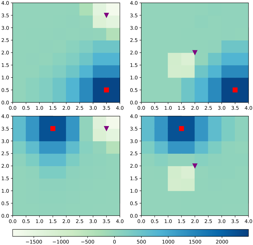

The implementation uses a polyhedral representation of regions and the values of the zero-sum normal-form games involved in the minimax operator at step 8 of Algorithm 1 are found by solving the corresponding linear program [50] using the SciPy library [51]. We have partitioned the state space of the game into two sets corresponding to the two possible local states of . The B-PWC VI algorithm converges after iterations when and takes s to complete. For each set in the partition of the state space, the BFCP of this set converges to the product of two grids. For the currently preferred parking spot of (red square) and coordinate of (purple triangle), the value function with respect to the coordinate of is presented in Fig. 6 (left) and shows that, the closer is to its preferred parking spot, the higher the (approximate) optimal value. The lightest-colour class is caused by an immediate crash, and its position follows from the observation function.
An (approximately) optimal strategy for is presented in Fig. 6 (right), where the colour intensity of an arrow is proportional to the probability of moving in that direction and the rotating arrow represents the parking action. We see that there are several choices that may not at first appear intuitive. As an example, moves left when in cell (top left), which is away from its current chosen parking spot. However, since is closer to its current parking spot, keeping away from this parking spot will avoid a crash with . In addition, under ’s transition function, the chosen parking spot will change with probability at each step, so with high probability will be able to park before can reach it and a crash can occur.
7 Policy iteration
It is known that, for MDPs, PI algorithms generally converge faster than VI algorithms, since policy improvement can jump over policies directly [52]. Motived by this fact, in this section we show how PI can be used to approximate the values and optimal strategies of an NS-CSG with respect to a discounted accumulated reward objective . Our algorithm takes ideas from recent work [18], which proposed a new PI method to solve zero-sum stochastic games with finite state spaces, and is the first PI algorithm for CSGs with Borel state spaces and with a convergence guarantee. Our PI algorithm ensures that the strategies and value functions generated during each iteration never leave a finitely representable class of functions. In addition, when computing values of CSGs, efficiencies are gained over alternative algorithms as there is no need to solve normal-form games, which is required by our B-PWC VI and Pollatschek-Avi-Itzhak’s PI algorithm [27], nor to solve MDPs, which adds complexity to Hoffman-Karp’s PI algorithm [26]. This results in cheaper computations and faster convergence over these alternatives, as for PI over VI for MDPs.
7.1 Operators, functions and solutions
Before presenting the algorithm, the following operators, functions and solutions are proposed. Let be a constant such that and , which will be used to distribute the discount factor between policy evaluation and policy improvement of the two agents.
Operators for Max-Min and Min-Max. Before introducing operators for Max-Min and Min-Max, we require the notion of a stationary Stackelberg (follower) strategy for , which is a stochastic kernel , i.e., such that for . This strategy is introduced only for the PI algorithm and implies that makes decisions conditioned on the current state and the current choice of , i.e. action distribution , and thus allows us to split the maximum and minimum operations of the two agents. We denote by the set of all stationary Stackelberg strategies for .
Definition 11 (Operator for the Max-Min value)
For strategy of and function , we define the operator such that for and :
where .
Definition 12 (Operator for the Min-Max value)
For Stackelberg (follower) strategy of and function , we define the operator such that for and :
where .
Unlike the classical PI algorithms by Hoffman and Karp [26] and Pollatschek and Avi-Itzhak [27], following [18], our PI algorithm separates the policy evaluation and policy improvement of the maximiser () and the minimiser () through the use of the operators of Definition 11 and Definition 12, respectively. To track the value functions after performing policy evaluation of and , our PI algorithm introduces value functions and . In addition, the value functions and are introduced to avoid the oscillatory behavior of the Pollatschek and Avi-Itzhak PI algorithm [27], thus ensuring convergence, and are updated only during policy improvement. The role of is to split the discount factor such that all the operators corresponding to policy evaluation and policy improvement of the two agents are contraction mappings, which then ensures convergence.
Two function representations. We next define two classes of functions, which play a key role in characterizing the functions and strategies generated during each iteration of our PI algorithm.
Definition 13 (CON-PWL Borel measurable function)
A function is a constant-piecewise-linear (CON-PWL) Borel measurable function if there exists a BFCP of such that, for each , for , and generates where , a BFCP of , such that for :
- 1.
is constant for where ;
- 2.
is B-PWL for .
Definition 14 (CON-PWC stochastic kernel)
A function is a constant-piecewise-constant (CON-PWC) stochastic kernel if there exists a BFCP of such that, for each , for , and generates where , a BFCP of , such that for :
- 1.
is constant for where ;
- 2.
is B-PWC for .
Fig. 7 presents an example of a CON-PWL Borel measurable function and CON-PWC stochastic kernel over a region. We now show that these two functions can be represented by finite sets of vectors. Each CON-PWL Borel measurable function can be represented by a finite set of vectors such that for and , where is a BFCP of for using Definition 13 and is a BFCP of , and again using Definition 13 is such that, over each region , is linear in given . Similarly using Definition 14, each CON-PWC stochastic kernel can be represented by a finite set of vectors such that for and , where is a BFCP of for using Definition 14, is a BFCP of , using Definition 14 is such that, over each region , is constant in given .
Maximum or minimum solutions. We introduce a criterion for selecting the maximum or minimum solution over a region, by which the strategies from policy improvement are finitely representable.
Definition 15 (CON- solution)
Let be a CON-PWL Borel measurable function. Using Definition 13 there exists a BFCP of for . Now, for each , if there exists such that:
for , and is a strategy of such that for , then is a constant- (CON-) solution of over .
Definition 16 (CON- solution)
Let be a Borel measurable function. If there exists a BFCP of where, for each , is constant for and there exists such that:
for , and is a Stackelberg strategy for such that for , then is a constant- (CON-) solution of over .
7.2 Minimax-action-free PI
We now use the operators for the Max-Min and Min-Max values (Definitions 11 and 12) to derive a PI algorithm called Minimax-action-free PI (Algorithm 3) for strategy synthesis for NS-CSGs with Borel state spaces. Our algorithm closely follows the PI method of [18] for finite state spaces, but has to resolve a number of issues due to the uncountability of the underlying state space and the need to ensure Borel measurability at each iteration. To overcome these issues we (i) introduce CON-PWL Borel measurable functions (Definition 13) and CON-PWC Borel measurable strategies (Definition 14) to ensure measurability and finite representability; (ii) work with CON- and CON- solutions (Definition 15 and (Definition 16) for policy improvement to ensure that the strategies generated are finitely representable and consistent; and (iii) propose a BFCP iteration algorithm (Algorithm 4) and a BFCP-based computation algorithm (Algorithm 5) to compute a new BFCP of the state space and the values or strategies over this BFCP. We also provide a simpler proof than that presented in [18], which does not require the introduction of any new concepts except those used in the algorithm.
Initialization. The Minimax-action-free PI algorithm is initialized with strategies and for each player, which are uniform distributions over available actions/state-action pairs, i.e., for all and for all , and four -valued functions, , , , i.e., for all and for all , and Algorithm 4 gives one BFCP for each strategy and function,
The algorithm. An iteration of the Minimax-action-free PI is given in Algorithm 3. As shown later, the order and frequency by which the possible four iterations of Algorithm 3 are run do not affect the convergence, as long as each is performed infinitely often. This permits an asynchronous implementation of the Minimax-action-free PI algorithm, as discussed in [18] and for its single-agent counterparts in [53].
For each of the four iterations, Algorithm 4 provides a way to compute new BFCPs and the results below demonstrate that, over each region of these BFCPs, the corresponding computed strategies and value functions are either constant, PWC or PWL. Therefore, we can follow similar steps to our VI algorithm (see Algorithm 1) to compute the value functions of these new strategies and value functions (see Algorithm 5). The idea is to first compute the BFCPs , , , , and via Algorithm 4 and then use them to compute strategies and value functions using Algorithm 5. For instance, if policy improvement of is chosen at iteration then we proceed as follows. First, new BFCPs are computed via Algorithm 4. Second, procedure of Algorithm 5 is performed. In this step we take each region , let , then take one state , and compute a BFCP of such that is constant over and for . Third, take one and find that minimises . Fourth, we let for and , which is a CON- solution of over by Lemma 9 and is CON-linear in and . Finally, we copy the other strategies and value functions for the next iteration.
Representation closures. The following lemmas show the strategies and value functions generated during each iteration of the Minimax-action-free PI algorithm are closed under B-PWC, CON-PWL and CON-PWC functions, and are thus finitely representable.
Lemma 6 (Evaluation closure for )
If is a PWC stochastic kernel, are CON-PWL Borel measurable and policy evaluation of is performed (procedure ), then is B-PWC.
Proof
Suppose is a PWC stochastic kernel and are CON-PWL Borel measurable. Since is a PWC stochastic kernel, there exists a constant-BFCP of for . Since is a CON-PWL Borel measurable function, there exists a BFCP of satisfying the properties of Definition 13 for . Therefore is constant on each region of the BFCP . We can similarly show that is constant on each region of the BFCP , where is a BFCP of from Definition 13 for . Consider the policy evaluation of (procedure ). Using Definition 11 we have that is constant on each region of the BFCP , which also implies that is Borel measurable. Since and are bounded, then is also bounded as required.
Lemma 7 (Improvement closure for )
If are CON-PWL Borel measurable and policy improvement of is performed (procedure ), then is a PWC stochastic kernel, and is B-PWC.
Proof
Suppose are CON-PWL Borel measurable functions. Using [46, Chapter 18.1] and Definition 13 it follows that the function is Borel measurable. Note that, over each region of , is constant in given , and PWL in given (where and are from Lemma 6), and therefore is CON-PWL.
Let and be a BFCP of satisfying the properties of Definition 13 for . Every state in each region of the BFCP has the same set of available actions for and same strategy that maximises on a region of . Therefore, using the CON- solution in Definition 15, the strategy of :
is constant on each region of , which also implies that is Borel measurable. Since is a PWC stochastic kernel, then Lemma 6 implies that is B-PWC as required.
Lemma 8 (Evaluation closure for )
If are B-PWC and is a CON-PWC stochastic kernel and policy evaluation of is performed (procedure ), then is CON-PWL Borel measurable.
Proof
Suppose and are B-PWC and is a CON-PWC stochastic kernel. Using [46, Chapter 18.1] it follows that is B-PWC. In view of the B-PWC function in Theorem 2, for each the function:
is B-PWC. Let be a BFCP of such that is constant on each region of for . It follows that is constant on each region of .
Next, let be a BFCP of satisfying the properties of Definition 14 for the CON-PWC stochastic kernel . For the BFCP of , we generate a BFCP of such that each region , induced by a region , is given by . Finally, consider the policy evaluation of . According to Definition 12, for , is constant in for a fixed , and PWL in for a fixed . Thus, is CON-PWL. Since and are bounded, Borel measurable, then so is by Definition 12 as required.
Lemma 9 (Improvement closure for )
If are B-PWC and policy improvement of is performed (procedure ), then is a CON-PWC stochastic kernel, and is CON-PWL Borel measurable.
Proof
Suppose are B-PWC. For the BFCP of , we generate a BFCP of such that each region in induced by a region is given by , where is from the proof of Lemma 8. Consider the policy improvement of (procedure ). According to Definition 12, by using the CON- solution in Definition 16, for , the Stackelberg strategy of :
is constant in for a fixed , and PWC in for a fixed . Thus, is CON-PWC. Since is a CON-PWC stochastic kernel, then Lemma 8 implies that is CON-PWL Borel measurable as required.
By fusing Lemmas 6, 7, 8 and 9 we can prove that the strategies and value functions generated during each iteration of Algorithm 3 never leave a finitely representable class of functions, and Algorithm 4 constructs new BFCPs such that the strategies and value functions after one iteration of the Minimax-action-free PI algorithm remain constant, PWC, or PWL on each region of the constructed BFCPs.
Theorem 3 (Representation closure)
In any iteration of the Minimax-action-free PI algorithm (see Algorithm 3), if
- 1.
are B-PWC and is a PWC stochastic kernel;
- 2.
are CON-PWL Borel measurable and is a CON-PWC stochastic kernel;
then so are , , , , and , respectively, regardless of which one of the four iterations is performed.
Proof
7.3 Convergence analysis and strategy computation
We next prove the convergence of the Minimax-action-free PI algorithm by showing that there exists an operator from the product space of the function spaces over which , , and are defined to itself, which is a contraction mapping with a unique fixed point, one of whose components is the value function multiplied by a known constant. The proof closely follows the steps for finite state spaces given in [18], but is more complex due to the underlying uncountable state space and the need to deal with the requirement of Borel measurability and finite representation of strategies and value functions.
Convergence analysis. Given PWC and CON-PWC , we define the operator such that:
| (2) |
where we assume are B-PWC, are CON-PWL, and the four operators , , and represent the four iterations of the Minimax-action-free PI algorithm from lines 3 to 16, and are defined as follows.
- 1.
corresponds to the policy evaluation of (procedure ) where for any :
(3) and is B-PWC using Lemma 6.
- 2.
corresponds to the policy improvement of (procedure ) where for any :
(4) and is B-PWC using Lemma 7.
- 3.
corresponds to the policy evaluation of (procedure ) where for any :
(5) and is CON-PWL Borel measurable using Lemma 8.
- 4.
corresponds to the policy improvement of (procedure ) where any :
(6) and is CON-PWL Borel measurable using Lemma 9.
For the spaces and , we consider the norm , and for the space the norm . We next require the following properties of these norms, which follow from [18].
Lemma 10
For any and :
Proof
Consider any . The norm for the space implies that for any :
| (7) | |||||
| (8) |
from which we have:
| (9) |
Exchanging with in (7) and (8) derives an inequality similar to (9), and combining it with (9) leads to the inequality:
| (10) |
for any . Since and are bounded, Borel measurable, so is by [46, Chapter 18.1], i.e., . Thus, since (10) holds for any :
The second inequality of the lemma can be proved following the same steps for .
Using the above operators and results, we are now in a position to prove the convergence of the Minimax-action-free PI algorithm.
Theorem 4 (Convergence guarantee)
If each of the four iterations of the Minimax-action-free PI algorithm (Algorithm 3) from lines 3 to 16 is performed infinitely often, then the sequence generated by the algorithm converges to .
Proof
We prove each component satisfies a contraction property. Suppose that are B-PWC and are CON-PWL Borel measurable.
- 1.
- 2.
- 3.
- 4.
For , since , by the sup-norm for :
rearranging (14) where the final inequality follows from similar arguments used in (13).
Next we prove that is a contraction mapping using the above inequalities. More precisely, by definition, see (2), we have:
where the final inequality follows from (11), (13), (12) and (14).
Therefore, since and assuming is PWC and is CON-PWC, we have that is a contraction mapping for . Now since is a complete metric space with respect to the sup norm, we conclude that has a unique fixed point . In view of (3)–(6), this fixed point satisfies for each :
| (15) | ||||
| (16) | ||||
| (17) | ||||
| (18) |
By combining (15)–(18), we have for each :
from which (16) and (18) can be simplified to:
implying that equals:
Thus, we have , which completes the proof.
Strategy computation. Next, introducing a criterion for selecting the minimax solution over a region, we compute the strategies for the agents based on the function returned by the Minimax-action-free PI algorithm.
Definition 17 (CON- solution)
Let . If there exists a BFCP of where, for each : for there exists a pair of probability measures and for such that for , and , are such that and for , then is a constant- (CON-) solution of over .
Lemma 11 (PWC strategies)
If , where is from iteration of the Minimax-action-free PI algorithm, and achieves the maximum and the minimum in Definition 10 for and all via a CON- solution, then and are PWC stochastic kernels.
Proof
By Theorems 3 and 4, is B-PWC. For any , the function is B-PWC by Theorem 2. Let be a BFCP of such that is constant on each region of for , and be a BFCP of such that is constant on each region of . Then, for and , the function , where:
for , is constant in each region of . Therefore, there exists a CON- solution of and, since is a BFCP, the result follows.
8 Conclusions
We have proposed a novel modelling formalism called neuro-symbolic concurrent stochastic games (NS-CSGs) for representing probabilistic finite-state agents with neural perception mechanisms interacting in a shared, continuous-state environment. NS-CSGs have the advantage of allowing for the perception of a complex environment to be synthesised from data and implemented via NNs, while the safety-critical decision-making module is symbolic, explainable and knowledge-based. We constrain the interface of the neural perception so that agents can reason symbolically using percepts, representing (exactly) learnt subregions of the continuous environment.
For zero-sum discounted cumulative reward problems, we proved the existence and measurability of the value function of NS-CSGs under Borel measurability and piecewise constant restrictions. We then presented the first computationally practical B-PWC VI and Minimax-action-free PI algorithms with finite representations for computing the values and optimal strategies of NS-CSGs, assuming a fully observable setting, by proposing B-PWC, CON-PWL and CON-PWC functions.
The B-PWC VI algorithm is, at the region level, the same as VI for finite state spaces, but involves, at each iteration, a division of the uncountable state space into a possibly refined finite set of regions (i.e., a BFCP). This is because taking the same action in two distinct states of some region in the current BFCP can yield states that need not be observationally equivalent. The Minimax-action-free PI algorithm requires multiple divisions of the uncountable state space into BFCPs at each iteration. We resolve a number of technical issues to apply [18], which ensures convergence, and, by not requiring the solution of normal-form games or MDPs at each iteration, reduces computational complexity. However, implementation of the Minimax-action-free PI algorithm is more challenging, requiring a distributed, asynchronous framework. We illustrated our approach by modelling a dynamic vehicle parking problem as an NS-CSG and synthesising approximately optimal values and strategies using B-PWC VI.
Future work will involve improving efficiency of the algorithms, generalising to more complex classes of neural perception mechanisms by exploiting preimage approximations [54], and moving to equilibria-based (nonzero-sum) properties, where initial progress has been made in a simpler setting of finite unfolding of our NS-CSG model [40]. We are also planning to extend the approach to two-sided partially observable neuro-symbolic POSGs, based on a recently proposed one-sided variant, which exploits a finite representation that generalises -vectors to approximate value computation [19], and for which online strategy synthesis methods have been developed [55].
Acknowledgements. This project was funded by the ERC under the European Union’s Horizon 2020 research and innovation programme (FUN2MODEL, grant agreement No. 834115).
References
- [1] D. Silver, A. Huang, C. Maddison, A. Guez, L. Sifre, G. Van Den Driessche, J. Schrittwieser, I. Antonoglou, V. Panneershelvam, M. Lanctot, et al., Mastering the game of Go with deep neural networks and tree search, Nature 529 (7587) (2016) 484–489.
- [2] S. Shalev-Shwartz, S. Shammah, A. Shashua, Safe, multi-agent, reinforcement learning for autonomous driving, arXiv:1610.03295 (2016).
- [3] J. Gupta, M. Egorov, M. Kochenderfer, Cooperative multi-agent control using deep reinforcement learning, in: Proc. 16th Int. Conf. Autonomous Agents and Multiagent Systems (AAMAS’17), Springer, 2017, pp. 66–83.
- [4] L. S. Shapley, Stochastic games, PNAS 39 (10) (1953) 1095–1100.
- [5] R. Yan, X. Duan, Z. Shi, Y. Zhong, J. Marden, F. Bullo, Policy evaluation and seeking for multi-agent reinforcement learning via best response, IEEE Trans. Automat. Contr. 67 (4) (2022) 1898–1913.
- [6] M. Kwiatkowska, G. Norman, D. Parker, G. Santos, Automatic verification of concurrent stochastic systems, Form. Methods Syst. Des. (2021) 1–63.
- [7] R. Lowe, Y. Wu, A. Tamar, J. Harb, P. Abbeel, I. Mordatch, Multi-agent actor-critic for mixed cooperative-competitive environments, in: Proc. 31st Int. Conf. Neural Information Processing Systems (NIPS’17), Curran Associates Inc., 2017, pp. 6382–6393.
- [8] M. E. Akintunde, E. Botoeva, P. Kouvaros, A. Lomuscio, Verifying strategic abilities of neural-symbolic multi-agent systems, in: Proc. 17th Int. Conf. Principles of Knowledge Representation and Reasoning (KR’20), IJCAI Organization, 2020, pp. 22–32.
- [9] L. D. Raedt, S. Dumancic, R. Manhaeve, G. Marra, From statistical relational to neural-symbolic artificial intelligence, in: Proc. 29th Int. Conf. Artificial Intelligence (IJCAI’20), IJCAI Organization, 2020, pp. 4943–4950.
- [10] G. Anderson, A. Verma, I. Dillig, S. Chaudhuri, Neurosymbolic reinforcement learning with formally verified exploration, in: Proc. 34th Int. Conf. Advances in Neural Information Processing Systems (NeurIPS’20), Curran Associates, Inc., 2020, pp. 6172–6183.
- [11] J. Van Der Wal, Discounted Markov games: Generalized policy iteration method, J. Optim. Theory Appl. 25 (1) (1978) 125–138.
- [12] B. Tolwinski, Newton-type methods for stochastic games, in: Differential games and applications, Springer, 1989, pp. 128–144.
- [13] J. Filar, K. Vrieze, Competitive Markov decision processes, Springer, 1997.
- [14] J. Perolat, B. Scherrer, B. Piot, O. Pietquin, Approximate dynamic programming for two-player zero-sum Markov games, in: Proc. 32nd Int. Conf. Machine Learning (ICML’15), Vol. 37, PMLR, 2015, pp. 1321–1329.
- [15] D. Bertsekas, Abstract dynamic programming, Athena Scientific, 2018.
- [16] M. Kwiatkowska, G. Norman, D. Parker, G. Santos, R. Yan, Probabilistic Model Checking for Strategic Equilibria-Based Decision Making: Advances and Challenges, in: 47th Int. Symp. Mathematical Foundations of Computer Science (MFCS’22), Vol. 241 of LIPIcs, Schloss Dagstuhl – Leibniz-Zentrum für Informatik, 2022, pp. 4:1–4:22.
- [17] P. Kumar, T.-H. Shiau, Existence of value and randomized strategies in zero-sum discrete-time stochastic dynamic games, SIAM. J. Control. Optim. 19 (5) (1981) 617–634.
- [18] D. Bertsekas, Distributed asynchronous policy iteration for sequential zero-sum games and minimax control, arXiv:2107.10406 (2021).
- [19] R. Yan, G. Santos, G. Norman, D. Parker, M. Kwiatkowska, Partially observable stochastic games with neural perception mechanisms, in: Proc. 26th Int. Symp. Formal Methods (FM’24), LNCS, Springer, 2024.
- [20] N. Brown, A. Bakhtin, A. Lerer, Q. Gong, Combining deep reinforcement learning and search for imperfect-information games, in: Proc. 34th Int. Conf. Advances in Neural Information Processing Systems (NeurIPS’20), Curran Associates, Inc., 2020, pp. 17057–17069.
- [21] V. Kovařík, M. Schmid, N. Burch, M. Bowling, V. Lisý, Rethinking formal models of partially observable multiagent decision making, Artif. Intell. 303 (2022) 103645.
- [22] A. Maitra, T. Parthasarathy, On stochastic games, J. Optim. Theory Appl. 5 (4) (1970) 289–300.
- [23] A. Nowak, Optimal strategies in a class of zero-sum ergodic stochastic games, Math. Methods. Oper. Res. 50 (3) (1999) 399–419.
- [24] A. Nowak, Universally measurable strategies in zero-sum stochastic games, Ann. Probab. 13 (1) (1985) 269–287.
- [25] O. Hernández-Lerma, J. Lasserre, Zero-sum stochastic games in borel spaces: average payoff criteria, SIAM. J. Control. Optim. 39 (5) (2000) 1520–1539.
- [26] A. Hoffman, R. Karp, On non-terminating stochastic games, Manage Sci. 12 (5) (1966) 359–370.
- [27] M. A. Pollatschek, B. Avi-Itzhak, Algorithms for stochastic games with geometrical interpretation, Manage. Sci. 15 (7) (1969) 399–415.
- [28] J. Křetínskỳ, E. Ramneantu, A. Slivinskiy, M. Weininger, Comparison of algorithms for simple stochastic games, Inf. Comput. 289 (2022) 104885.
- [29] J. Eisentraut, E. Kelmendi, J. Křetínskỳ, M. Weininger, Value iteration for simple stochastic games: Stopping criterion and learning algorithm, Inf. Comput. 285 (2022) 104886.
- [30] H. Yu, D. Bertsekas, A mixed value and policy iteration method for stochastic control with universally measurable policies, Math. Oper. Res. 40 (4) (2015) 926–968.
- [31] H. Yu, On convergence of value iteration for a class of total cost Markov decision processes, SIAM. J. Control. Optim. 53 (4) (2015) 1982–2016.
- [32] I. Hogeboom-Burr, S. Yuksel, Comparison of information structures for zero-sum games and a partial converse to Blackwell ordering in standard borel spaces, SIAM. J. Control. Optim. 59 (3) (2021) 1781–1803.
- [33] A. Basu, Ł. Stettner, Zero-sum Markov games with impulse controls, SIAM. J. Control. Optim. 58 (1) (2020) 580–604.
- [34] A. Cosso, Stochastic differential games involving impulse controls and double-obstacle quasi-variational inequalities, SIAM. J. Control. Optim. 51 (3) (2013) 2102–2131.
- [35] K. Chatterjee, R. Ibsen-Jensen, Qualitative analysis of concurrent mean-payoff games, Inf. Comput. 242 (2015) 2–24.
- [36] N. Basset, M. Kwiatkowska, C. Wiltsche, Compositional strategy synthesis for stochastic games with multiple objectives, Inf. Comput. 261 (2018) 536–587.
- [37] T. Brázdil, V. Forejt, J. Krčál, J. Křetínskỳ, A. Kučera, Continuous-time stochastic games with time-bounded reachability, Inf. Comput. 224 (2013) 46–70.
- [38] J. Fearnley, M. N. Rabe, S. Schewe, L. Zhang, Efficient approximation of optimal control for continuous-time Markov games, Inf. Comput. 247 (2016) 106–129.
- [39] R. Yan, G. Santos, G. Norman, D. Parker, M. Kwiatkowska, Strategy synthesis for zero-sum neuro-symbolic concurrent stochastic games, arXiv:2202.06255 (2022).
- [40] R. Yan, G. Santos, X. Duan, D. Parker, M. Kwiatkowska, Finite-horizon equilibria for neuro-symbolic concurrent stochastic games, in: Proc. 38th Conf. Uncertainty in Artificial Intelligence (UAI’22), AUAI Press, 2022, pp. 2170–2180.
- [41] S. Sharma, S. Sharma, A. Athaiya, Activation functions in neural networks, IJEAST 6 (12) (2020) 310–316.
- [42] K. Matoba, F. Fleuret, Computing preimages of deep neural networks with applications to safety, openreview.netforum?id=FN7BUOG78e (2020).
- [43] J. Kemeny, J. Snell, A. Knapp, Denumerable Markov Chains, Springer, 1976.
- [44] K. D. Julian, M. J. Kochenderfer, A reachability method for verifying dynamical systems with deep neural network controllers, arXiv.1903.00520 (2019).
- [45] D. Ayala, O. Wolfson, B. Xu, B. Dasgupta, J. Lin, Parking slot assignment games, in: Proc. 19th ACM SIGSPATIAL Int. Conf. Advances in Geographic Information Systems (GIS’11), ACM, 2011, p. 299–308.
- [46] H. L. Royden, P. Fitzpatrick, Real analysis (fourth edition), Macmillan New York, 2010.
- [47] K. Parthasarathy, Probability measures on metric spaces, AMS., 1967.
- [48] J. Reif, Universal games of incomplete information, in: Proc. 11th ACM Symp. Theory of Computing (STOC’79), ACM, 1979, pp. 288–308.
- [49] J. Reif, The complexity of two-player games of incomplete information, J. Comput. Syst. Sci. 29 (1984) 274–301.
- [50] J. von Neumann, O. Morgenstern, H. Kuhn, A. Rubinstein, Theory of Games and Economic Behavior, Princeton University Press, 1944.
- [51] P. Virtanen, R. Gommers, T. Oliphant, M. Haberland, T. Reddy, D. Cournapeau, E. Burovski, P. Peterson, W. Weckesser, J. Bright, S. van der Walt, M. Brett, J. Wilson, K. Millman, N. Mayorov, A. Nelson, E. Jones, R. Kern, E. Larson, C. Carey, İ. Polat, Y. Feng, E. Moore, J. VanderPlas, D. Laxalde, J. Perktold, R. Cimrman, I. Henriksen, E. Quintero, C. Harris, A. Archibald, A. Ribeiro, F. Pedregosa, P. van Mulbregt, SciPy 1.0 Contributors, SciPy 1.0: Fundamental Algorithms for Scientific Computing in Python, Nature Methods 17 (2020) 261–272.
- [52] D. Bertsekas, Abstract dynamic programming, Athena Scientific, 2022.
- [53] D. Bertsekas, H. Yu, Q-learning and enhanced policy iteration in discounted dynamic programming, Math. Oper. Res. 37 (1) (2012) 66–94.
- [54] X. Zhang, B. Wang, M. Kwiatkowska, Provable preimage under-approximation for neural networks, in: Proc. 30th Int. Conf. Tools and Algorithms for the Construction and Analysis of Systems (TACAS’24), Vol. 14572 of LNCS, Springer, 2024, pp. 3–23.
- [55] R. Yan, G. Santos, G. Norman, D. Parker, M. Kwiatkowska, HSVI-based online minimax strategies for partially observable stochastic games with neural perception mechanisms, in: Proc. 6th Learning for Dynamics & Control Conference L4DC’24, Vol. 424 of Proceedings of Machine Learning Research, PMLR, 2024, pp. 80–91.