Renormalization group analysis of the finite 2DXY model with fourfold anisotropy: Application to the magnetic susceptibility of a ferromagnetic ultrathin film
Abstract
The renormalization group equations describing a finite 2DXY system with fourfold anisotropy are solved in two steps, in order to study the magnetic transition to paramagnetism in an ultrathin film. First, the equations are linearized near the critical coupling . This allows integration constants to be evaluated at the fixed point, and the tuning of the constants to represent a ferromagnetic ultrathin film. An exact solution of the linearized equations confirms that a finite-size Kosterlitz-Thouless (KT) transition occurs in the presence of weak fourfold anisotropy, and that an Ising transition occurs for strong anisotropy. The behaviour of a given system, and the crossover region between these two types of transitions, is determined by the system parameters through the product of an anisotropy parameter and the logarithm of the system size. The linearized RG equations are not quantitatively reliable across the extended temperature range of the finite-size transition, but they do define the parameter space where a second approach, where the fourfold anisotropy is treated as a perturbation, is valid. This perturbative treatment provides a quantitative determination of the renormalized exchange coupling, vortex density, and anisotropy throughout the transition. In particular, the coupling has a universal point of inflection where vortex-antivortex pairs unbind (as opposed to a “universal jump”), and goes to zero asymptotically in the paramagnetic state, as is expected for a finite system. These results are used to calculate the magnetic susceptibility as the system moves from one dominated by spin waves to one dominated by a free vortex gas. The presence of anisotropy makes it necessary to include both the susceptibility due to fluctuations of the magnitude of the magnetization, and due to angular fluctuations of the magnetization about a fourfold easy axis. A comparison to recent measurements of the magnetic susceptibility of ultrathin Fe/W(001) films suggests that a detailed quantitative analysis of the experimental results can provide information on vortex formation, the disappearance of anisotropy, and dissipative processes in the finite-size KT transition of a real system.
I Introduction
Nearly half a century after BerezinskiiBerezinskii 1971, Kosterlitz and ThoulessKosterlitz and Thouless 1973, and Kosterlitz Kosterlitz 1974, introduced the ideas underlying the transition of a spin system between phases supporting excitations of different topologies, there has been a resurgence of interest in topological spin textures in material systems. Topological spin textures of current interest include chiral “bubbles” in perpendicularly magnetized filmsJenkins et al. 2019, vortices bounded within a ferromagnetic microstructureSugimoto et al. 2011; Kuepper et al. 2007, 2D skyrmionsYu et al. 2010 in ferromagnetic and antiferromagnetic layers, 3D skyrmions in crystalsMühlbauer et al. 2009; Münzer et al. 2010, as well as the chiral domain wall spin textures in these systemsClarke et al. 2008; Güngördü et al. 2016. There is great interest in the phase diagrams and transitions between the topological phasesRybakov et al. 2013, as well as in the non-equilibrium dynamics of the topological excitationsFu et al. 2018. These investigations are driven both by fundamental questions in the larger area of topological materials, and by the prospect of potential applications in spintronics.
Within the context of this larger field of work, the simpler, archetypical 2DXY ferromagnetic system originally considered by Kosterlitz and ThoulessKosterlitz and Thouless 1973; Kosterlitz 1974; Kosterlitz 2016 can provide insight into basic questions relevant to many of the systems that support topological spin textures. These include the effects of dissipation and relaxation towards equilibriumHe et al. 2009; Ozeki et al. 2003; Rojas and Rutenberg 1999, finite-size effectsBramwell and Holdsworth 1993; Chung 1999, fluctuations near transitionsArchambault et al. 1998 and the influence of perturbations from an ideal symmetry as may be provided by, for example, defectsHoll et al. 2020 and anisotropiesJosé et al. 1977.
Despite these opportunities, there is a relatively small literature reporting experimental studies of 2DXY ferromagnetic films focused on the Kosterlitz-Thouless (KT) transition and vortex dynamics. Experimental work has focused instead on superconductorsGoldman 2013 and layered three dimensional antiferromagnetsAls-Nielson et al. 1993; Bramwell et al. 1995; Cuccoli et al. 2003. For the most part, studies of ferromagnetic films consist of magnetization studies of ferromagnetic films grown on (001)-oriented metallic substratesTaroni et al. 2008, where a non-Ising magnetization exponent was reported and only later interpreted as the signature of a finite-size KT transitionBramwell and Holdsworth 1993. Early indications that experimental measurements of the magnetic susceptibility displayed the characteristic form of a KT transition in such filmsElmers et al. 1996 were made quantitative only recentlyAtchison et al. 2019, using Fe/W(001) ultrathin films. This opens the path for further quantitative experimental studies using the magnetic susceptibility, aimed at a better understanding of topological spin textures using this simple realization of a topological phase transition.
The first step is to make contact between the experimental thin film results and theoretical predictions through a quantitative determination of the exchange and anisotropy parameters in a 2DXY system. Kosterlitz and ThoulessKosterlitz and Thouless 1973; Kosterlitz 1974 treated the infinite, isotropic system and introduced the KT transition. Bramwell, Holdsworth and coworkersBramwell and Holdsworth 1993; Bramwell and Holdsworth 1994; Archambault et al. 1998 investigated the finite, isotropic system and identified essential finite-size effects and the finite-size KT transition with separate characteristic temperatures for the formation of vortex-antivortex pairs and for unbinding of the pairs to form a free vortex gas. José et al.José et al. 1977; José 2013 derived the renormalization group equations for the infinite, anisotropic system with an -fold, in-plane anisotropy. They showed that the system is Ising-like for , and has a KT transition when . A system with microscopic fourfold anisotropy flows to a second order transition to paramagnetism with non-universal critical exponents that depend upon the strength of the anisotropy. For large anisotropy, there is a cross-over to 2D Ising exponents.
The finite, anisotropic 2DXY model with fourfold anisotropy has not been investigated in detail. Taroni et al.Taroni et al. 2008 have reported Monte Carol simulations as a function of the strength of the fourfold anisotropy, and of system size. They find a competition between the finite size effects and anisotropy. For small anisotropy, finite size effects prevail and the value of the effective critical exponent of the magnetization indicates that a finite-size KT transition occurs. As the anisotropy increases, the effective critical exponent crosses over to the 2D Ising value. The present article concentrates instead on solutions of the RG equations to provide a detailed description of the behaviour of an ultrathin ferromagnetic film with fourfold anisotropy. This is accomplished in two stages. In the first stage, the RG equations are expanded to lowest order about the critical coupling, when , and solved exactly. This allows appropriate physical parameters to be set, and makes contact with the previous findings for the finite, isotropic system. These results validate the use of a second approach within a large parameter space, where the fourfold anisotropy is treated as a perturbation. This method yields quantitative results for the effective exchange coupling, vortex density and screened fourfold anisotropy as a function of temperature and system size throughout the full temperature range of the finite-size transition. It shows that the coupling has a universal point of inflection where vortex-antivortex pairs unbind (as opposed to a “universal jump”), and goes to zero asymptotically in the paramagnetic state. The fourfold anisotropy also goes to zero smoothly just above the temperature where the vortex pairs unbind.
These quantities are then used to find two components of the magnetic susceptibility: an improved calculation of the longitudinal susceptibility due to fluctuations in the magnitude of the magnetizationArchambault et al. 1997, and, in addition, the transverse susceptibility due to fluctuations of the magnetization direction about an easy axis in the fourfold system. The appropriate combination of these susceptibilities give an excellent qualitative account of the experimental measurements of Atchison et al.Atchison et al. 2019 and suggest that a detailed quantitative comparison with the measurements can provide information on vortex formation, the disappearance of anisotropy, and domain processes in the finite-size KT transition of an experimental system.
II Renormalization group equations under geometric scaling
The 2DXY ferromagnetic spin model with a fourfold anisotropy is represented by the HamiltonianJosé et al. 1977
| (1) |
where is the bare nearest neighbour exchange coupling, is the angle the in-plane spin at lattice site makes with a fixed in-plane “easy” magnetic axis, and is the microscopic anisotropy energy for a fourfold in-plane anisotropy. The sum over is over nearest neighbours on a square lattice. The renormalization group (RG) equations under geometric scaling for this model have been derived by José et al.José 2013; José et al. 1977 using an approximation due to VillainVillain 1975 that is applicable for small anisotropy. After defining as the temperature-normalized exchange coupling, they find:
| (2) |
| (3) |
| (4) |
These equations are first order in the system variables and (see below), with corrections in the third order. is the scaling length, where the system size is in units of the nearest neighbour lattice constant. The temperature-normalized anisotropy is
| (5) |
Due to approximations made in the Villain model, the maximum value of corresponds to a clock model with effectively infinite anisotropy.José et al. 1977
The fugacity of a vortex, or the density of vortices, is given by
| (6) |
is a small parameter that is renormalized by the flow described by the RG equations. It has been introduced into the Villain model (where ), to create the generalized Villain model. In the regions , is renormalized to zero and is an irrelevant parameter. In the region , is renormalized to unity and is a relevant parameter. In this way, it can be shownJosé et al. 1977 that the generalized Villain model formally reproduces the results for an isotropic 2DXY system as described by the Villain model. By introducing , it was possible to display a dual symmetry between and in the anisotropic 2DXY model. This was instrumental in the original derivation of the RG equations.
While introducing was necessary, it is problematic when relating the system of equations to a physical system. This is because is a phenomenological, and not a physical, parameter. For this reason, it is useful to recast the equations in terms of the fugacity , and a modified, but still physical, anisotropy parameter that maintains the dual relation with :
| (7) |
A line of fixed points of the RG equations occurs when , regardless of the value of . A second line occurs when . José et al.José et al. 1977 have shown that, in an infinite system, this second line of fixed points mark second-order phase transitions for systems of different microscopic fourfold anisotropy. These transitions have non-universal exponents that depend upon the anisotropy, and, in the limit of strong anisotropy, cross over to 2D Ising transitions.
The RG equations (2) to (4) that include fourfold anisotropy will be solved for a finite system in two steps. In Section III, the equations are solved by expansion about the critical coupling . This is referred to as the “critical approximation” and is routinely used to study critical properties. This step is necessary because the fixed point is the only place where boundary conditions are known precisely. RG equations valid at the fixed points can be used to determine the values of constants of integration, and to tune parameters in the equations to values appropriate for ultrathin films. The solutions confirm that a finite-size KT transition can be preserved in the presence of fourfold anisotropy, and that, because the fixed point is approached only logarithmically in the system size , there is a large parameter space where the renormalization flow does not approach the critical point closely. In Section IV, a second approximation is used. This is referred to as the “perturbative approximation”. It is not as good close to the fixed point (where the flow does not proceed in a finite system), but is valid across the broad temperature range of the finite-size transition where the flow does proceed. This provides a more accurate calculation of the effective coupling, vortex density, anisotropy, and ultimately, the magnetic susceptibility.
III Renormalized coupling near the critical coupling, in the presence of fourfold anisotropy
III.1 Flow equations
This section extends previous workBramwell and Holdsworth 1993; Bramwell and Holdsworth 1994 by including the effects of fourfold anisotropy. The coupling in the RG equations is expanded about its value at the fixed point, to lowest order in the parameter :
| (8) |
| (9) |
This yields the equations to lowest order in for small :
| (10) |
with ,
| (11) |
| (12) |
Using eq.(11) and (12) to substitute for one power of and , respectively, eq.(10) can be written as a perfect differential that can be integrated to give
| (13) |
where is a constant of integration. Taking the ratio of eq.(11) and (12) gives an expression independent of that can be integrated to yield
| (14) |
where is a second constant of integration. The known parameter values at the fixed point require that
| (15) |
and indicate that an infinite system with bare anisotropy flows to a fixed point where .
The constant is determined by substituting eq.(14) into eq.(13) and using the known values at the fixed point, to give . This value describes a flow line leading to the fixed point. This value of therefore defines the separatrix between different types of flow leading away from this fixed point (for a system with this anisotropy). The flow for systems near the separatrix is investigatedKosterlitz 2016; Berlinsky and Harris 2019 by allowing the integration constant to deviate from the separatrix by a small amount proportional to the reduced temperature, , where gives flow on the separatrix to the phase transition represented by the fixed point. Then
| (16) |
whereGupta et al. 1988; Bramwell et al. 2001 and It can be shown11 1 D. Venus, unpublished that negative values of correspond to flow away from the fixed point to a low temperature phase with high anisotropy and vanishing vortex density (fugacity). Positive values of give flow to a high temperature phase with vanishing anisotropy and high vortex density. This type of behaviour led to the original identification of a topological transition at in the isotropic systemKosterlitz and Thouless 1973; Kosterlitz 1974.
Finally, the value of is used to complete the square in eq.(13) to yield an equation that describes the flow near the critical coupling:
| (17) |
III.2 Tuning to the physical parameters of the system
To follow the renormalization of a specific system with a specific value of fourfold anisotropy it is necessary to follow the flow line with the specific value of for this system.Berlinsky and Harris 2019 This value of is determined by the initial conditions for the system, where “(0)” indicates that renormalization begins at the microscopic level where . To accomplish this, all variables are expressed in terms of the initial value . In the case of , this requires using the definition of to substitute for the temperature:
| (18) |
In addition, the number of free parameters is reduced by introducing the ratio of the microscopic fourfold anisotropy to the bare exchange, , so that
| (19) |
Since is a phenomenological parameter, its value is not known at the microscopic level. To find a reasonable estimate for , the fugacity is expressed instead in terms of the energy of a vortex core, .
| (20) |
An approximate expression for the energy of a vortex core, derived from the Villain modelBerlinsky and Harris 2019 is . (Here only, is Euler’s constant.) Then, for the purpose of tuning the system,
| (21) |
When the initial conditions fall on the separatrix () for a system with a particular value of the microscopic anisotropy, the flow proceeds to the fixed point and the corresponding value of can be identified. According to eq.(17), this occurs when
| (22) |
After substituting from eq.(21) and (19), this equation can be solved for for the value of that characterizes the bare system, and the corresponding value of can be found using eq.(14):
| (23) |
The upper and lower root in eq.(22) correspond to whether or not . The condition divides these cases, and represents a system with initial conditions at the fixed point at . It presumably stays at the fixed point under geometric scaling.
Initial conditions for systems with a wide range of are collected in Table 1. It turns out that only the positive root of eq.(22) is relevant, as this root produces up to . Under the assumptions of the generalized Villain modelJosé et al. 1977, the maximum value of is unity. According to eq.(9), this implies a maximum value of . Therefore, table entries for are certainly not well-founded. Ultrathin metallic films on single-crystal substrates have anisotropies with the order of magnitude , giving . This is well within the range of validity of the generalized Villain model.
| 7.3 | 0 | 0.101 | 0.101 | 1.02 |
| 3.0 | 0.215 | 0.0790 | 0.0620 | 4.90 |
| 1.0 | 0.421 | 0.0625 | 0.0287 | 1.79 |
| 0.5 | 0.506 | 0.0566 | 0.0163 | 9.20 |
| 0.1 | 0.595 | 0.0512 | 0.00366 | 1.87 |
| 0.01 | 0.620 | 0.0497 | 3.81 | 1.89 |
| 0.001 | 0.623 | 0.0495 | 3.81 | 1.89 |
| 0 | 0.623 | 0.0495 | 0 | 0 |
III.3 Finite-size transition
To find the coupling for an anisotropic finite system of size , eq.(10) must be integrated up to . This is accomplished by solving the quadratic equations in eq.(17) for and , and substituting back into eq.(10) to give the integral equation
| (24) |
A standard transformation shows that this is an elliptic integral of the first kindAbramowitz and Stegun 1964. It is solved exactly in terms of the Jacobi elliptic functions in appendix A.
For an approximate solution for small values of , such as those appropriate for ultrathin films, it is useful to rewrite eq.(24) as the difference of squares.
| (25) |
For small enough , an excellent approximation22 2 The validity of this approximation is clear a posteriori from the fact that in a finite-size transition both and are not simultaneously small in comparison to ; that is, the system does not get close to the critical point. is to neglect the contribution from the term . (See section III. D.) Then, using the substitution results in an exact differential of arctangent. As the geometric scaling described by the RG equations removes the sensitivity to the initial value of , let . Then
| (26) |
This functional form is identical to that found by Bramwell and HoldsworthBramwell and Holdsworth 1993 for the isotropic system, with the substitution
| (27) |
so that, compared to the isotropic system, the effect of the anisotropy is to shift reduced temperatures by .
Whereas the second order transition in the infinite system with fourfold anisotropy occurs at the fixed pointJosé et al. 1977 , the renormalization flow in the finite system avoids the fixed point so that the condition occurs at the reduced temperature . (The subscript “c” refers to the critical approximation.) This condition no longer represents a sharp transition, but rather marks when the formation of vortex-antivortex pairs starts to be significant. According to eq.(26), when
| (28) |
Substituting the expression for from eq.(26) into eq.(17) leads to quadratic equations for and . The solutions are most usefully expressed in terms of the scaled variable :
| (29) |
| (30) |
Then
| (31) |
| (32) |

These expressions for and are plotted in fig.(1), using scaled variables that exhibit (near) universal curves. Each of the plots has a curve for and for . Only in part (c) for is there an indication that the curves do not overlap precisely. For , curves generated using the exact solutions in appendix A are indistinguishable within the linewidth from the the approximate solution shown in fig.(1).
The finite-size transition ends when the system moves to an endpoint where the vortex density gets very large due to the unbinding of the vortex-antivortex pairs, and the anisotropy is screened away. According to fig.(1), this occurs when , independent of system size. Following Bramwell and HoldsworthBramwell and Holdsworth 1993, this corresponds to , and according to eq.(26), occurs at33 3 The notation is used here, rather than as used in ref. 18, to reinforce that the separation of and is a finite-size effect.
| (33) |
In a finite system, the correlation length is limited by the system size. This implies that the correlation length is maximum near , where the paramagnetic vortex gas forms. In the presence of fourfold anisotropy, eq.(33) can be used to show that it scales as
| (34) |
Since is small for thin ferromagnetic films, the difference between this relation and the form found for the isotropic system, will be very difficult to observe.
These results confirm that the finite-size KT transition in ultrathin ferromagnetic films survives the inclusion of fourfold anisotropy, and that a second order transition is not expected. The effective coupling, correlation length, and transition points are those found previously for the isotropic system, if . The principle new finding is the expression in eq.(32) for .
However, it is also clear from fig.(1) that there are important quantitative problems with the calculated system properties. The effective exchange coupling goes to zero () before the vortex gas forms at (). The condition is marked in fig.(1a) by the circular dots for systems with sizes increasing by integer values of from 4 to 9. At larger values of the coupling becomes large and antiferromagnetic, a situation that is unphysical. Thus the calculation is certainly not reliable near , and is unlikely to be reliable outside the region near where is indeed a small expansion parameter. Another example can be seen in part (c) of the figure, where the anisotropy goes to zero with a discontinuity in slope and becomes complex above , rather than approaching zero as a smooth and continuous real function. These are indications that the critical approximation will not be sufficient for a quantitative description of the system across the full temperature range of the finite-size transition, including for the calculation of the magnetic susceptibility.
III.4 Limiting behaviours in the critical approximation
Although the critical approximation does not provide a quantitative description throughout the finite-size KT transition, it can provide guidance as to whether or not the system will flow away from the critical point towards a free vortex gas, or towards the critical point and a second order transitionJosé et al. 1977 that is characterized by either Ising exponents, or non-universal exponents. This question can be explored using the exact solution in the critical approximation developed in appendix A, where it is shown that the solution in terms of trigonometric functions in eq.(26) is replaced by
| (35) |
sn and cn are Jacobi elliptic functionsAbramowitz and Stegun 1964, and the function parameters for the finite 2DXY model with fourfold anisotropy are
| (36) |
The product of the system size and anisotropy in characterizes the system behaviour. The finite-size transition begins at , and the type of phase transition the system undergoes is determined by how it approaches the fixed point () as a function of the system size. As is outlined in appendix A, is determined by the condition
| (37) |
In this transcendental equation, is the complete elliptic integral of the 1st kindAbramowitz and Stegun 1964, and . These definitions imply that
| (38) |
To understand the critical behaviour, note that the complete elliptic integral can be represented to a high degree of accuracy by the functionAbramowitz and Stegun 1964
| (39) |
where and are slowly-varying polynomials with positive values. Substituting this in eq.(38) and solving for ,
| (40) |
When is small, , and the system is in the limit of small anisotropy. Then and the eq.(40) becomes
| (41) |
This has the form of eq.(28) and describes a system that approaches the fixed point logarithmically in and is described by a finite-size KT transition.
When approaches unity, and the system is in the limit of large anisotropy. Then and the singular part of eq.(40) is
| (42) |
This power law behaviour indicates a second order transition with critical exponent . To find , recall that is the value of at the fixed point where . In the limit of large anisotropy in the generalized Villain model, , so that
| (43) |
This value agrees with the analysis of Taroni et al.Taroni et al. 2008 for an infinite system, and represents the 2D Ising limit of the generalized Villain model . The fact the the correct 2D Ising value is underestimated is due to the limitation of the Villain model to small anisotropyJosé et al. 1977, and does not affect the conclusion that this is the Ising-like limit of the model.

The boundary where the system crosses over from 2nd order to finite-size KT behaviour depends upon what deviation from “pure” limiting behaviour is acceptable before the system is considered to be in a crossover region. A pragmatic approach is to begin with the condition where each of the product terms in eq.(40) are equal, or equivalently, when the two terms in eq.(39) are equal. This occurs whenAbramowitz and Stegun 1964 . Eq.(37) then indicates . Because of the definition of , this condition defines a line in the parameter space of vs. , and is marked by a solid line near the centre of fig.(2), dividing regions labelled “Ising-like” and “Finite-size KT”.
To investigate the power law behaviour moving toward the the boundary line from the region of large and , recognize that is a small parameter, and set
| (44) |
Substituting this and the association developed in eq.(43) into the divergent term in eq.(40) gives
| (45) |
The correction term in eq.(45) is of the form . It increases in size moving toward the boundary from large and , and makes a correction of about -9% at the boundary when a conservative value of is used. This represents a significant departure from pure power law behaviour, and is expected to cause an effective critical exponent to better describe the system. The size of the change in is difficult to determine in the present analysis, but it is consistent with the boundary lying within the crossover region. A dashed line further into the region labelled “Ising-like” is included in fig.(2) to indicate an approximate upper bound to the crossover region. It is set somewhat arbitrarily by the condition that the power law term in eq.(40) is twice the size of the exponential term.
The finite-size KT behaviour at the boundary line is investigated by assessing deviations from the correlation length given in eq.(34). From appendix A, , so that
| (46) |
is expandedAbramowitz and Stegun 1964 about in powers of , and terms up to on the right side of eq.(46) are retained. The resulting quadratic equation for is solved and the term in is isolated. This yields
| (47) |
For the boundary at in fig.(2), and the characteristic form of the correction length at a finite-size KT transition is modified by an increasing amount as the boundary is approached from the region of low and . The correction is +7% at the boundary. This is of a similar magnitude to the modification of the Ising-like correlation length at the boundary, and suggests that the boundary in fig.(2) is indeed roughly in the centre of the crossover region. A dashed line further into the region labelled “Finite-size KT” is included in fig.(2) to indicate an approximate lower bound to the crossover region. Again, it is set by the condition that the exponential law term in eq.(40) is twice the size of the power law term.
In the infinite system, there is no KT behaviour, but rather the 2nd order transition persists to low anisotropyJosé et al. 1977, where it exhibits non-universal critical exponents with . The exact solution of the RG equations in the critical approximation indicates that this type of transition no longer exists in the finite system, except perhaps as a qualitative explanation of the continuously varying effective critical exponents in the transition region. 44 4 As , eq.(35) can be expanded in hyperbolic functions as The second root leads to the Ising-like transition, and this root exists even when is finite. The first root exits only when , and can be shown to be the root for a 2nd order transition at low anisotropy. In addition, the product of the roots is dominated by the stronger, Ising-like root, so that the transition at low anisotropy is not expressed in a finite system.
A separate, but closely related, question is defining the parameter space where the description of the entire finite-size KT transition in the critical approximation is consistent with the results of the previous section. That is, what is the “Low D” region within which the approximation leading from eq.(25) to (26) is valid at rather than at ? Since eq.(46) and (38) differ only in having and subscripts , the analysis in eq.(47) can be applied directly. To maintain a similar correction of about 7% to the calculation of properties for the full transition requires . Using eq.(37), this gives as the boundary. This second solid line is marked on fig.(2) to define a region in the lower left corner where the Low D method of solving the RG equations is essentially equivalent to the exact solution. This region certainly contains the parameters describing ultrathin ferromagnetic films.
The dotted line in fig.(2) is discussed in the next section.
Fig.(2) summarizes a number of important conclusions concerning the observation of a finite-size KT transition in a real, finite system with fourfold anisotropy. First, the type of transition depends upon the product of the anisotropy and the system size in the combination , not just on the size of the anisotropy alone. Second, the second order transition with non-universal exponents , predicted for the infinite system, does not occur in the finite system. These observations do not contradict the findings of Taroni et al.Taroni et al. 2008, who found non-universal effective exponents for low anisotropy in simulations performed using a Monte Carlo technique. These effective exponents arise in the transition region in fig.(2) They used planar spins on a 2D square lattice with sites, so that . This system size is marked by the vertical dashed line in the figure. The lower dot on this line marks the value of for their calculation when . This was the largest anisotropy for which the calculated magnetization exhibited finite-size KT behaviour. The upper dot marks the value of when , the smallest anisotropy for which the calculated magnetization exhibited Ising-like behaviour. (No calculations are reported for anisotropy between these values.) As can be seen, the Monte Carlo simulations are in good agreement with the present analysis.
Comparing the values in Table I to those in fig.(2), it is clear that metallic, ferromagnetic thin film systems will always exhibit a finite-size KT transition. For other types of systems, neutron scattering experiments have been reported for a few magnetic, layered insulators with weak interlayer coupling, so that they behave as a 2DXY system at low temperature. For ferromagnetic Rb2CrCl4, it is estimatedTaroni et al. 2008 that (so that Table I gives ), and that the system size is limited by the interlayer coupling to about . These co-ordinates are indicated by the square in fig.(2), in a region where finite-size KT behaviour is expected, in agreement with the analysis of the neutron scattering measurements. A second example is antiferromagnetic K2FeF4, for which anomalous exponents have been observed.Thurlings et al. 1982 For this compound, is estimated to be 0.33 due to gaps in the magnon spectrumTaroni et al. 2008. The corresponding value of is indicated by the horizontal dashed line in the figure. The authors of the neutron scattering analysisThurlings et al. 1982 argue that the observed critical exponents are comparable to those of the 2D Ising model. According to fig.(2), this would imply a large system size of , despite the interlayer interactions that limit the range of 2D magnetic behaviour. On the other hand, Taroni et al.Taroni et al. 2008 point out that the measured value of is intermediate between the 2D Ising value (0.125) and the effective value for the finite 2DXY model (0.231). This suggests that the effective 2D system size is smaller, and that antiferromagnetic K2FeF4 sits within the transition region, consistent with fig.(2).
IV Renormalized coupling across the finite-size transition in the presence of fourfold anisotropy
IV.1 Flow equations
In order to explore the entire temperature range of the finite-size transition, it is better to retain the original RG equations and work directly with a normalized, effective coupling within the range . Then the RG equations are:
| (48) |
| (49) |
| (50) |
| (51) |
Expressed in these variables, the flow equations have a fixed point at .
These equations are not amenable to a closed solution. However, an approximation is suggested by the exact solution in the critical approximation in appendix A. Because the renormalization flow approaches the fixed point logarithmically in (see eq.(29)), finite systems do not get very close to the fixed point. Rather, they follow a path where in the pertinent range of reduced temperature. From eq.(A.19) and (A.18),
| (52) |
where dn() is the third Jacobi elliptic functionAbramowitz and Stegun 1964. This ratio has its largest value when , or . In this limit dn() sech, and
| (53) |
When is small, the term in in eq.(49) can be neglected, and the resulting solutions for and can be used to find as a perturbation through the ratio of eq.(50) and (51). Choosing gives =1.27 as the upper limit. The resulting boundary for this approximation is shown on fig.(2) as the dotted line, where it almost overlaps the boundary for the “Low D” solution. This gives a sizeable parameter space where this approach is valid, and certainly includes the ferromagnetic thin films that are the focus of the present analysis.
This approach will be termed the “perturbative approximation”. The relevant equations in this approximation are
| (54) |
| (55) |
| (56) |
It is important to reiterate that although eq.(54) to (56) do not display the fixed point of the original RG equations, they are a very good approximation in the region some distance from the fixed point where the renormalization flow carries a finite system.
Rearranging eq.(55) as an expression for , and substituting for one power of in eq.(54), leads to a relation between exact differentials that can be integrated as
| (57) |
The integration constant can be identified by expanding this equation about and comparing to eq.(17) in the region where they are both valid. This gives
| (58) |
Incorporating this in eq.(57), provides a final expression for the fugacity in the perturbative approximation:
| (59) |
IV.2 Finite-size transition
Substituting the expression for from eq.(59) into eq.(54), and separating variables gives
| (60) |
Because of the presence of , this integral cannot be performed analytically. However, the denominator is well-behaved so long as , and various approximations are instructive. These approximations are illustrated in fig.(3), where the term in square brackets in eq.(60) is plotted. The solid line is the exact function, and the purely quadratic function is the critical approximation for small used in the previous section. The figure makes it clear why this approximation is unreliable near , where the free vortex gas forms.

A simple and effective representation of is achieved by piecewise polynomials. In the range , the polynomial is used. Then eq.(60) has the form
| (61) |
where with and . This integral is given in appendix B in eq.(B.9). Its qualitative form is more easily seen in the limit , where the expression simplifies to
| (62) |

This coupling is closely related to eq.(26) in the critical approximation, but represents an important qualitative change. While there is only a modest difference near , the behaviour at is very different. The implicit equation for includes a term in that rules out solutions for . Thus the system approaches the limit of vanishing exchange coupling () asymptotically in .
In the range in fig.(3), is reasonably approximated by the polynomial . This is again of the form in eq.(61), but the algebra is more complicated. The result is given in appendix B in eq.(B.13), and is qualitatively similar to eq.(62) with the substitution of a generalized expression for
| (63) |
where is a function that arises from matching the two polynomial approximations at , and is given in eq.(B.14).
These various expressions for are compared in fig.(4a) as a function of for parameters appropriate for ultrathin Fe/W(001) filmsAtchison et al. 2019,55 5 The value of is relevant only in that it is small enough for the approximation in eq.(54) to (56) to hold, since and occur only in the combination .: and . The solid curve is a numerical integration of the relation in eq.(60). The polynomial approximation to it is given by the long dash line. As can be seen, the closed expressions in eq.(B.9) and (B.13) reproduce the exact result very well. The two curves nearly overlap; the deviation is greatest at the matching point and for large as . The effective exchange coupling approaches asymptotically, as is appropriate for a finite system, and there is no region where the coupling becomes antiferromagnetic.
The result in the critical approximation, given by eq.(26), is also shown as a short dash line in fig.(4a). Bramwell et al.Bramwell and Holdsworth 1993 have shown, using the critical approximation, that the effective critical exponent of the magnetization, given by
| (64) |
has a universal value 0.231…, and that this prediction is well supported by experiment.Taroni et al. 2008. Comparing the two approximations, there is a small shift in the region near , but the slopes of the curves are very nearly the same.66 6 Compare eq.(62) and (26). For this reason, the value of the effective critical exponent will not be affected. Fig.(4b) shows for a range of system sizes.
IV.3 Width of the finite-size transition
The onset of the formation of vortex-antivortex pairs continues to occur when the value of the coupling is equal to the value at the fixed point (). In the perturbative approximation, an expression for can be found from eq.(B.9), as it applies for . As , a small angle approximation for the tangent at an angle slightly less than yields the solution given in eq.(B.10) in appendix B. When , this becomes

| (65) |
The values of are plotted against the system size in fig.(5a), using a solid line. The dashed lines are the results of the critical approximation in eq.(28) and (33). The scaling properties of in the perturbative approximation are revealed by replotting fig.(4b) as a function of the scaled parameter in fig.(5b). A second scaling point occurs at the point of inflection of all of the curves, at77 7 Here, the symbol does not represent a critical exponent. , at which point independent of the system size. For the finite system, this point of steepest descent is all that remains of the instantaneous jump in the coupling observed at in the isotropic, infinite system. It is identified as and the values are plotted in fig.(5a) using a solid line.
The scaling can be used with eq.(65) to determine the scaling of the correlation length
| (66) |
This displays the exponential singularity associated with a KT transition. The constant in the exponential factor has been altered by a factor of from that found in the critical approximation. The prefactor to the exponential has no singularity and does not affect the scaling behaviour substantially within the range where the estimate applies.
IV.4 Screening of the anisotropy
With solutions for and derived under the condition that , it is now possible to solve for as a perturbation using eq.(56). First, note from eq.(59) that is the square root of the function , where
| (67) |
Using this relation, eq.(56) can be written as
| (68) |
As the variables and are separated, integration leads to
| (69) |
The integration constant can be determined in the limit , where the critical and perturbative approximations are both valid. Then, from eq.(14),
| (70) |
since at . This notation is understood to mean that is a constant in the integral and takes the value appropriate for the system size of the endpoint . According to eq.(59),
| (71) |
Using these results, eq.(69) can be written as
| (72) |
| (73) |

The fugacity from eq.(59) and the anisotropy from eq.(72) are plotted against in fig.(6a) and (6b), respectively. Each fugacity curve rises smoothly with no marker of either the beginning () or end () of the finite-size KT transition, although the presence of the transition can be seen through the scaling at . Because the exchange coupling never renormalizes to zero in these finite systems, bound vortex pairs and free vortices always coexist. The inset shows the same data, again plotted against , but now normalized as . This gives a near universal curve for , in good agreement with the critical approximation in fig.(1b) in this range.
The anisotropy plotted in fig.(6b) approaches zero smoothly and continuously, where it has the functional form of an exponential of the exponential function. In the inset, the anisotropy is scaled by to allow direct comparison with fig.(1c). The near universal curve for observed in the critical approximation is seen here as well. The anisotropy extends beyond , especially for smaller system sizes. This again reflects the fact that smaller systems contain a more truncated distribution of vortex sizes.
V The magnetic susceptibility
V.1 Contribution due to fluctuations in the scalar magnetization
Archambault et al.Archambault et al. 1997 have studied the magnetic susceptibility in a finite-size, isotropic 2DXY system, and demonstrated that a broad peak occurs as the spatial range over which the effective coupling varies diverges until it is limited by the system size. Their analysis uses the harmonic 2DXY model (which is almost equivalent to the Villain model) on a square lattice of spins with no explicit fourfold anisotropy term. The lattice spacing is unity. They find that the vector magnetization has a well-defined scalar magnitude in the spin wave region at low temperature. The magnetization rotates “slowly” in the isotropic XY plane, so that in finite spin systems the scalar magnetization is a well-defined quantity on experimental time scales despite the lack of anisotropy. They suggest that when magnetic properties such as the magnetic susceptibility or critical behaviour are measured in an applied field, the field pins the direction of the magnetization so that the relevant fluctuations are in the magnitude of the magnetization.
Defining the scalar magnetization in terms of the in-plane unit spins at site i,
| (74) |
they calculate the susceptibility per spin, , as the fluctuations in the scalar magnetization:
| (75) |
They work in units where the Boltzmann constant is unity. In the low temperature spin wave region, the magnetization has the form
| (76) |
where is the 2D Green’s function for the square lattice, evaluated at the origin (see appendix C). The second moment of the scalar magnetization is
| (77) |
so that
| (78) |
This expression is generalized to higher temperature in the range of the finite-size Kosterlitz-Thouless transition by replacing the bare coupling by the effective coupling as determined by the renormalization group equations. A choice must be made for the value to be used in the final term in eq.(78), as it is outside the sum over . Because is dominated by fluctuations at small wavevector, the choice is made.
Archambault et al.Archambault et al. 1997 show that a series expansion of the exponential in converges very quickly. When only the first term beyond unity is kept, then the susceptibility can be divided into a part due to spin waves,
| (79) |
and a part due to vortices,
| (80) |
Because a characteristic experimental thin film system sizeAtchison et al. 2019 is , eq.(79) and (80) for the susceptibility can be evaluated in the continuum limit. This is outlined in appendix C.

A comparison of the magnetic susceptibility calculated using for a system with fourfold anisotropy, determined in both the critical and perturbative approximations in the previous sections, is shown in fig.(7). The system parameters are and . (A small jump in the solid curve near occurs at the point where the perturbative approximation for moves from one piecewise polynomial to another.) Both curves are in qualitative agreement, in that the susceptibility is small in the spin wave region, begins to increase near , where vortex pairs begin to form, and has a broad peak over the entire range of the finite-size transition.
There are, however, important quantitative differences. In the critical approximation, the susceptibility has a larger amplitude and reduced full-width at half maximum, and the position of the peak is significantly below . The curve terminates just past its peak, at the point where and eq.(79) and (80) diverge. Although the high temperature tail of the curve is predicted to have an exponential dependence on from general arguments leading to eq.(34), it is not possible to demonstrate this characteristic functional dependence of the vortex gas. In contrast, in the perturbative approximation asymptotically so that the system remains ferromagnetic, and the expressions for the susceptibility remain well defined. The position of the curve maximum is very nearly at and the form of the high temperature tail can be determined in detail. These differences, and the changes in the values of and , are important for quantitative fitting of experimental data to extract magnetic properties and properties of the vortex distribution.
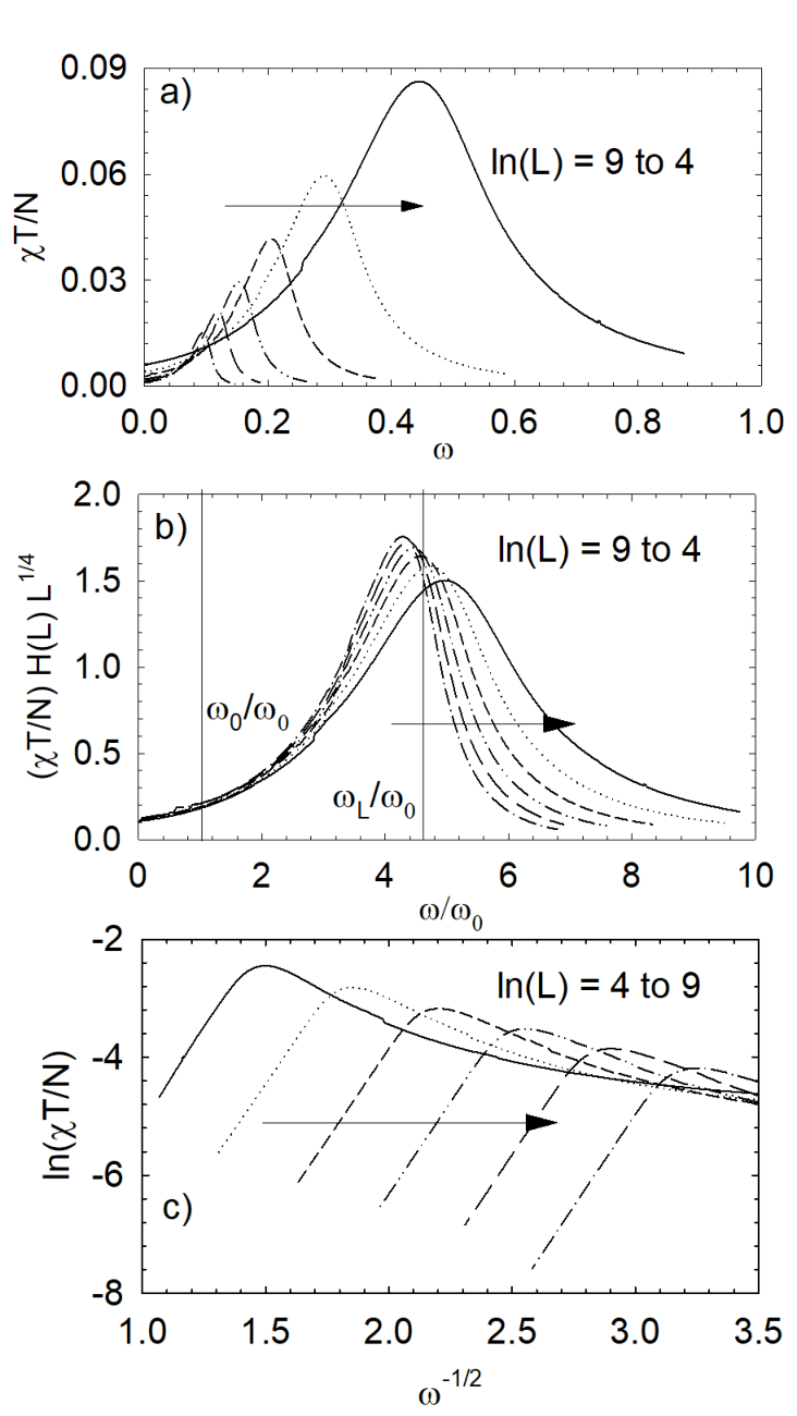
For these reasons, further analysis of the magnetic susceptibility is restricted to that calculated using the perturbative approximation. The sum of the spin and vortex contributions are shown in fig.(8a) for a range of system sizes. It can be seen that the susceptibility gets narrower as the system size increases. If it were not normalized by a factor of in the figure, the susceptibility per spin, , would increase dramatically as the system size increased. In the infinite, isotropic 2DXY model, the susceptibility scales as at the KT transition.Kosterlitz and Thouless 1973; Kosterlitz 1974 In a finite system, the transition begins instead at the reduced temperature , and, as is shown in appendix C, the vortex susceptibility at this transition point scales as
| (81) |
In this expression, the explicit logarithmic term arises from essential finite size effects in the magnetization, and the factor of is due to finite-size effects in the coupling. As can be seen in fig.(5a), the dependence of on depends strongly on the approximations made in solving the RG equations. In the critical approximation, the expression for in eq.(28) gives
| (82) |
In the perturbative approximation, the dependence of on the size of the system can be expressed as a continued approximation in , using eq.(65). This gives
| (83) |
where . This expression contains higher order logarithmic corrections. In part (b) of the figure, the susceptibilities are scaled by , and plotted against . The data collapse at is very good. The fact that both the critical and perturbative approximations give the same order for the simple logarithmic correction provides some confidence that this order is correct. The correction varying as is necessary, as the scaling at is much better when it is included than when it is omitted. However, the exact order of this correction is likely sensitive to details of the perturbative approximation, such as the use of piecewise polynomials, and the truncation of the continued approximation for in orders of after two terms. The expression for the magnetic susceptibility itself has involved approximations in moving from eq.(78) to eq.(80). The spin part of the susceptibility scales differently than the vortex part, but this does not effect the overall scaling because it is so much smaller (see appendix C).
This plot makes it clear that the susceptibility peak becomes narrower in larger system sizes because the high temperature side is cut off more sharply. This is due to the inclusion of larger vortices that more completely destroy the magnetization stabilized by finite-size effects. It can also be seen that while the peak maxima occur near , where has a point of inflection, the peak position disperses somewhat with size.
The high temperature tail of the susceptibility is expected to scaleKosterlitz 1974 as . According to eq.(66), it will therefore depend on reduced temperature as , independent of system size. This behaviour is illustrated in fig.(8c). The slope of the curves ranges from 6.17 to 6.24 for system sizes of = 5 to 9, respectively. If the predicted value of at is used, then the slope is expected to be 5.88. Because the slopes in fig.(8c) are determined significantly above , the value of is likely to be less than 1/4 and dependent on the temperature range.Als-Nielson et al. 1993 If this is indeed the case, then a value of is derived from the slopes.
V.2 Contribution due to fluctuations in the magnetization direction
With the inclusion of explicit fourfold anisotropy, the direction of the magnetization may no longer be determined by the applied field, but rather by the magnetic easy axes. It is then important to distinguish between the susceptibility with a small field applied along the magnetization (as in the previous section), and with a field applied perpendicular to the magnetization. Experimental measurements are expected to include both.
The anisotropy can be represented by an anisotropy field , and a small oscillating field can be simultaneously parallel and perpendicular to an easy axis. The effective field along which the scalar magnetization is aligned in equilibrium is
| (84) |
For definiteness, the x-axis is chosen along an easy axis, and the angle of the magnetization is measured from this axis. Applying a field along the y-axis and measuring the magnetic response along the y-axis gives the measured susceptibility tensor component :
| (85) |
where the anisotropy field is derived from the anisotropy energy density88 8 This section continues to use the same units as ref. 32. For SI units factors of the saturation magnetization and magnetic permeability must be included. .
| (86) |
Recalling that the effective field is by definition parallel to the magnetization in equilibrium, the reciprocal of the effective susceptibility component can be expressed in planar circular components as
| (87) |
is just the (reciprocal of the) susceptibility due to fluctuations of the scalar magnetization calculated in the previous section for the finite-size KT transition. For consistency of notation with previous sections, this susceptibility will be referred to simply as . Combining the results of eq.(85) to (87), the experimentally measured susceptibility per spin is
| (88) |
Since the sum in the second term in eq.(1) represents the total anisotropy energy of the system, dividing this sum by gives the anisotropy energy per spin. The sum itself is evaluated through the block spin renormalization procedure that is halted when the system is represented by a single block of size , anisotropy parameter and spin orientation . The anisotropy energy per spin can therefore be written as99 9 Again, in this section units with and lattice constants of unit length are used.
| (89) |
Using planar circular co-ordinates once again to perform the partial derivatives in eq.(86) and (85) yields
| (90) |
With the oscillating field applied along the y-axis, the low temperature domains with magnetization aligned along the easy axis parallel to the y-axis have , and
| (91) |
This is the result from the previous section.
For domains aligned along the easy axis parallel to the x-axis, at low temperatures where the anisotropy persists, and the susceptibility is given by
| (92) |
As the temperature increases, decreases and goes to zero near . In the absence of anisotropy in eq.(90), the scalar magnetization aligns with the applied field, giving . Then the susceptibility is once again given by eq.(91). For a sample with a distribution of both domain types, the susceptibility will be given by a linear combination of the limiting forms and .
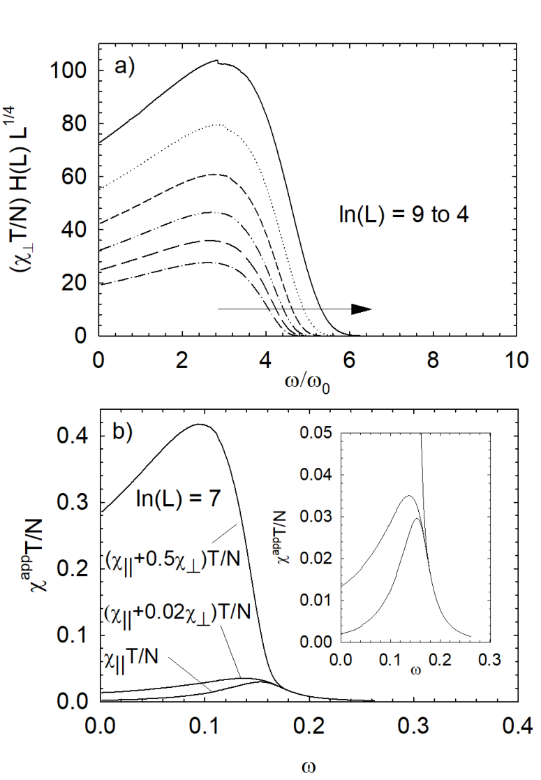
The transverse susceptibility in eq.(92) is plotted in fig.(9a) for a range of system sizes. The susceptibility is scaled in the same way as the plot of in fig.(8b) to allow comparison. It can be seen that the transverse susceptibility due to angular fluctuations about the easy axis is much larger than the longitudinal susceptibility due to fluctuations of the magnitude of the magnetization. In addition, the low temperature limit (near ) of increases much more quickly as the system size is decreased, than does . However, as the anisotropy is screened near and above , goes quickly to zero and the longitudinal susceptibility is dominant. As a result, the high temperature tail of the susceptibility displays the characteristic functional form of a KT transition regardless of the domain orientations at low temperature. This is consistent with an isotropic paramagnetic vortex gas.
This behaviour can be seen in part (b) of the figure. The curve labeled represents a low temperature domain with the magnetization aligned with the applied field, whereas that with a small admixture of represents a situation where the field direction is slightly misaligned with the magnetization. These two curves are shown more clearly in the insert to the figure, using a magnified scale. These curves look very much like the experimental curves categorized as Type I in the experimental investigation of Fe/W(001) films by Atchison et al.Atchison et al. 2019 The third curve, with a large admixture of of , represents a situation where there are equal portions of low temperature domains aligned along each of the two easy axes. This curve is similar to those categorized as Type II in the experimental study, including the observed factor of roughly ten in amplitude compared to Type I measurements. Although the precise numerical factors for the admixtures in fig.(9b) are not fitted, but rather chosen for illustrative purposes, the similarity between these first-principles calculations and the experimental measurements is very encouraging. These results support the suggestion that the difference between Type I and Type II measurements in the finite-size KT transition has to do with the low temperature domain distribution in the film and the distinction between and introduced by the fourfold anisotropy.
VI Conclusions
The magnetic response of the finite, anisotropic 2DXY model has been investigated using the renormalization group equations, by extending previous work on the infinite, anisostropic model and the finite, isotropic model. An exact solution of the RG equations in the critical approximation confirms previous numerical simulations that showed that a finite-size KT transition is preserved for low anisotropy, and a 2D Ising transition occurs at high anisotropy. The boundary line between these two behaviours depends upon the product of the anisotropy and system size through the system parameter . In a more restricted region of parameter space, the effect of fourfold anisotropy can be incorporated into the description of the isotropic system by the simple substitution . The temperature range within which the critical approximation is valid is considerably narrower than the finite-size KT transition itself, so that the coupling, fourfold anisotropy and magnetic susceptibility found in this way provide qualitative insight, but are not quantitatively reliable.
The results of the critical approximation validate solving the RG equations by treating the fourfold anisotropy as a perturbation. This approximation proves to be quantitatively reliable across the full temperature width of the finite-size KT transition, so long as the system parameter is small enough. A principle finding is that the coupling no longer exhibits physically unreasonable behaviour (moving from ferromagnetic to antiferromagnetic, and then diverging), but rather approaches zero asymptotically. The universal jump of the coupling seen in an infinite system becomes instead a universal inflection point of steepest descent where and . At , the unbinding of vortex-antivortex pairs becomes significant. The dependence of on system size implies that the correlation length and magnetic susceptibility retain the exponential temperature dependence characteristic of the KT transition. Furthermore, the fourfold anisotropy calculated in the perturbative approximation no longer exhibits an unphysical cusp, or becomes complex, near
The perturbative approximation gives an improved calculation of the effective exchange coupling, vortex density and anisotropy throughout the range of the finite-size KT transition in a ferromagnetic film with fourfold anisotropy. These in turn permit an improved calculation of the magnetic susceptibility, , due to the fluctuations in the magnitude of the magnetization. The improved results for the anisotropy and scalar magnetization are used to find the transverse susceptibility, , for angular fluctuations of the magnetization about an easy axis. Together, these susceptibility components give a more complete account of the magnetic response of the 2DXY model with fourfold anisotropy.
An initial comparison to the measurements of the magnetic susceptibility of Fe/W(001) ultrathin films is very encouraging. Suitable combinations of and are in good qualitative agreement with, for instance, fig. (1a) and (4a) in Atchison et al.Atchison et al. 2019. In particular, the two distinct shapes of the measured susceptibility termed Type I and Type II by those authors agree well with the combinations of and expected for situations where low temperature magnetic domains are aligned along single or multiple fourfold easy axes. Because near , both types of measurements exhibit the exponential dependence on temperature characteristic of a finite-size KT transition, indicating an isotropic high temperature phase. The experimental value of in the temperature range where the exponential dependence is observed is consistent with the present calculations, where . The implication is that careful fitting of Type I measurements can be used to understand details of vortex pair formation, and fitting of Type II measurements can be used to study the evolution of the anisotropy in the finite-size KT transition. This process is underway.
These results open numerous opportunities to study spin wave and vortex properties in an ultrathin ferromagnetic film. The RG treatment of the 2DXY model uses an effective medium approach, where the presence of vortices and bound vortex pairs alters the medium in which spin waves propagate. Therefore, these calculations can be a basis for interpreting the imaginary, dissipative components of the measured susceptibility. For example, can be used to determine the energy barrier to dissipative domain switching due to an applied field. Also, the variation of the domain wall energy and activation energy for domain wall pinning in the effective medium are determined by a combination of and . These dissipative process can be studied as the system moves from a low temperature system dominated by spin wave excitations to one dominated by vortices. The imaginary component of the susceptibility above the transition may provide information on the dynamics of the vortex gas itself. These investigations are underway.
Appendix A. Exact solution in the critical approximation
Beginning with eq.(24)
| (A.1) |
a standard transformation will show that this is an elliptic integral of the first kind. Since the flow is from a larger positive initial value of to a final value near , it is advantageous to write the integral in a form where it is dominated by the endpoint near . Then it is insensitive to the initial value and the scaling properties will not depend it, as is expected. This can be accomplished through the co-ordinate transformation . Then
| (A.2) |
Letting ,
| (A.3) |
where . This is a well-known transformation of the standard form of elliptic integrals of the first kindAbramowitz and Stegun 1964, obtained by letting . Then
| (A.4) |
where . At this point, as the value of is not important, let . Recalling that the upper limit of is (in units of the lattice constant), the integral becomes
| (A.5) |
with the elliptic integral of the first kind, , and .
The expression in eq.(A.5) can be formally written in a way that isolates by using the inverse elliptic functionAbramowitz and Stegun 1964 . If
| (A.6) |
then the inverse function is defined as
| (A.7) |
In the present case,
| (A.8) |
| (A.9) |
Although the inverse elliptic integral cannot be solved analytically, some general results can be extracted by employing the Jacobi elliptic functions , defined asAbramowitz and Stegun 1964
| (A.10) |
| (A.11) |
First note that, for the present problem,
| (A.12) |
where is a constant for a given system of size and anisotropy . Then the expression for can be written as
| (A.13) |
To determine the functional form of and in this temperature range, eq.(17) can be combined with eq.(A.13) to give
| (A.14) |
Using the propertyAbramowitz and Stegun 1964 , and reversing the sign of the square in ,
| (A.15) |
Recalling the definition of , the second term on the left side cancels with the last two terms on the right. The third Jacobi elliptic functionAbramowitz and Stegun 1964,
| (A.16) |
is used to substitute for . Then the square root of both sides can be taken to give
| (A.17) |
This quadratic equation, and the corresponding quadratic equation for , can be solved for two physical roots:
| (A.18) |
| (A.19) |
The condition for the beginning of the finite-size transitionBramwell and Holdsworth 1993 is that , or . According to eq.(A.13), this corresponds to
| (A.20) |
where
| (A.21) |
defines the value of reduced temperature where the transition begins. The periodic propertyAbramowitz and Stegun 1964 of the function requires that
| (A.22) |
with the complete elliptic integral of the first kind. Combining the definition of in eq.(A.12) with these results gives an expression for the transition point.
| (A.23) |
In the limit of vanishing fourfold anisotropy, , and , so that finite-size transition point is in agreement with eq.(28). The end of the finite-size transition, where the vortices unbind, occurs whenBramwell and Holdsworth 1993 at . This condition is given by eq.(A.13) as
| (A.24) |
This implies . In the limit where there is no anisotropy, this agrees with eq.(33). The correlation length at and above is
| (A.25) |
and has the functional form expected for a KT transition.
Appendix B. Polynomial approximation of the integral expression for
The critical approximation uses the quadratic approximation . When this expression is used in eq.(60) of the perturbative approximation, the integral for become
| (B.1) |
where
| (B.2) |
with and . This standard integral yields the expressionAbramowitz and Stegun 1964
| (B.3) |
For comparison, the solution for the critical approximation, given by eq.(26), is
| (B.4) |
A better representation of is given by two piecewise polynomials. For , the integral expression for in eq.(60) is well-approximated by
| (B.5) |
The integral in is now of the form
| (B.6) |
with , and , and the discrimanent . The solution isAbramowitz and Stegun 1964
| (B.7) |
Evaluating this expression in the limit is well-behaved, and gives
| (B.8) |
After considerable algebra, the following closed expression for is obtained:
| (B.9) |
In the limit that , this reduces to eq.(62).
When , the coupling reaches the critical value where the finite-size KT transition begins. This is denoted by . This condition can be found by using a small angle approximation for the tangent function in eq(B.9), when the angle is just less than . Then
| (B.10) |
In the limit where , this reduces to eq.(65).
For , the polynomial approximation to in fig.(3) is given by
| (B.11) |
This leads to an integral for of the same form as eq.(B.6), but with and
| (B.12) |
After considerably more algebra, the result is
| (B.13) |
In this expression,
| (B.14) |
The complicated expression for arises due to matching the two quadratic approximations at . Note that both of the arctangent functions return angles in the 2nd quadrant.
Appendix C. Evaluation of the susceptibility
In the low temperature, spin wave limit of the harmonic model, Archambault et al.Archambault et al. 1997 show that the magnetization is of the form
| (C.1) |
where is the Green’s function propagator for the square lattice, evaluated at the origin. That is,
| (C.2) |
evaluated at . In this Fourier sum over wavevectors in 2D,
| (C.3) |
A discrete evaluation gives
| (C.4) |
whereBramwell et al. 2001 , as before. Because of this logarithmic dependence on system size, the 2DXY model has intrinsic finite-size effects, with
| (C.5) |
converging very slowly even for macroscopic .
VI.1 The vortex susceptibility
Since the experimental systemAtchison et al. 2019 has , the continuum limit of the sum should be a very good approximation. Because is a function of the scalar in the perturbative approximation, there is no differentiation between the in-plane and axes, and the integral can be most easily performed in circular, planar co-ordinates . In moving from a square to a circular system while maintaining the number of spins,
| (C.6) |
where is the maximum value of . The minimum value of , corresponding to the bare lattice spacing before geometric scaling, is . In the continuum limit, the vortex susceptibility in eq.(80) is
| (C.7) |
Using the change of variables ,
| (C.8) |
Finally, substituting for and ,
| (C.9) |
Recall that this is an equation for because of the implicit temperature dependence of . In the low temperature limit, the coupling renormalizes very slowly with size, so that it is essentially constant. Then the vortex susceptibility is identically zero.
To display the scaling properties of the vortex susceptibility, the first term in eq.(C.7) is integrated by parts. One portion of the integration by parts cancel exactly with the second term in eq.(C.7), leaving
| (C.10) |
Here the dependence of the susceptibility on through the coupling is displayed explicitly. The universal point where the finite-size transition begins, regardless of the system size, is , where In the finite, anisotropic system, eq.(B.9) is used to give
| (C.11) |
Eq.(65) is used to substitute for the expression within the argument of the sine function.
| (C.12) |
Because is small, the sine function is essentially unity. Replacing these results, and the expression for from eq.(C.4), into eq.(C.10) produces
| (C.13) |
This integral contains only powers of , and this is well-behaved near , as can be seen in fig.(4). The integral over will cancel the prefactor of . The expected scaling with size at the onset of the finite-size transition is therefore approximately
| (C.14) |
The detailed scaling of the susceptibility depends on the dependence of on . As can be seen in fig.(5a), this depends upon the approximations made in the solution of the RG equations.
VI.2 The spin wave susceptibility
In the continuum limit, the expression for the spin wave susceptibility in eq.(79) can be written as
| (C.15) |
This can be integrated by parts by identifying
| (C.16) |
so that
| (C.17) |
In this expression, limits the sum to the spins within a disc of radius . A numerical summationArchambault et al. 1997 shows that
| (C.18) |
with . Letting
| (C.19) |
| (C.20) |
Collecting these together,
| (C.21) |
Since , the lower limit in the first line of eq.(C.21) is smaller than the upper limit, and is neglected. In the remaining integral, the expression can be evaluated by isolating the term in the geometric scaling equations (B.9) or (B.13) and (B.14) that give .
| (C.22) |
Again, in the low temperature limit, scales very slowly with size, so that the coupling is essentially constant. This means the integral portion of the spin wave susceptibility is zero because the limits of the integral are essentially the same. The first term is then equivalent to
| (C.23) |
in agreement with Archambault et al. Archambault et al. 1997
Acknowledgements.
Financial support for this work was provided by the Natural Sciences and Engineering Research Council of Canada (NSERC) through the Discovery program. I am indebted to Sung-Sik Lee of McMaster University for many useful discussions, and thank the referees for constructive comments.References
- Berezinskii (1971) V. L. Berezinskii, JETP 32, 493 (1971).
- Kosterlitz and Thouless (1973) J. M. Kosterlitz and D. J. Thouless, J. Phys. C: Solid State Phys. 6, 1181 (1973).
- Kosterlitz (1974) J. M. Kosterlitz, J. Phys. C: Sold State Phys. 7, 1046 (1974).
- Jenkins et al. (2019) A. Jenkins, M. Pelliccione, G. Xi, X. Ma, X. Li, K. L. Wang, and A. C. Bleszynski, Phys. Rev. Materials 3, 083801 (2019).
- Sugimoto et al. (2011) S. Sugimoto, Y. Fukuma, S. Kasai, T. Kimura, A. Barman, and Y. C. Otani, Phys. Rev. Lett 106, 197203 (2011).
- Kuepper et al. (2007) K. Kuepper, M. Buess, J. Raabe, C. Quitmann, and J. Fassbender, Phys. Rev. Lett. 99, 167202 (2007).
- Yu et al. (2010) X. Z. Yu, Y. Onose, N. Kanazawa, J. H. Park, J. H. Han, Y. Matsui, N. Nagaosa, and Y. Tokura, Naure 465, 901 (2010).
- Mühlbauer et al. (2009) S. Mühlbauer, B. Binz, F. Jonietz, C. Pfleiderer, A. Rosch, A. Neubauer, R. Georgii, and P. Böni, Science 323, 915 (2009).
- Münzer et al. (2010) W. Münzer, A. Neubauer, T. Adams, S. Mühlbauer, C. Franz, F. Jonietz, R. Georgii, P. Böni, B. Pedersen, M. Schmidt, A. Rosch, and C. Pfleiderer, Phys. Rev. B 81, 041203(R) (2010).
- Clarke et al. (2008) D. J. Clarke, O. A. Tretiakov, G. W. Chern, Y. B. Bazaliy, and O. Tchernyshyov, Phys. Rev. B 78, 134412 (2008).
- Güngördü et al. (2016) U. Güngördü, R. Nepal, O. A. Tretiakov, K. Belashchenko, and A. A. Kovalev, Phys. Rev. B 93, 064428 (2016).
- Rybakov et al. (2013) F. N. Rybakov, A. B. Borisov, and A. N. Bogdanov, Phys. Rev. B 87, 094424 (2013).
- Fu et al. (2018) X. Fu, S. D. Pollard, B. Chen, B. K. Yoo, H. Yang, and Y. Zhu, Science Advances 4, 3007 (2018).
- Kosterlitz (2016) J. M. Kosterlitz, Rep. Prog. Phys. 79, 1 (2016).
- He et al. (2009) Y. Y. He, B. Zheng, and N. J. Zhou, Phys. Rev. E 79, 021107 (2009).
- Ozeki et al. (2003) Y. Ozeki, K. Ogawa, and N. Ito, Phys. Rev. E 67, 026702 (2003).
- Rojas and Rutenberg (1999) F. Rojas and A. D. Rutenberg, Phys. Rev. E 60, 212 (1999).
- Bramwell and Holdsworth (1993) S. T. Bramwell and P. C. W. Holdsworth, J. Phys.: Condens. Matter 5, L53 (1993).
- Chung (1999) S. G. Chung, Phys. Rev. B 60, 11761 (1999).
- Archambault et al. (1998) P. Archambault, S. T. Bramwell, J. Y. Fortin, P. C. W. Holdsworth, S. Peysson, and J. F. Pinton, J. Appl. Phys. 83, 7234 (1998).
- Holl et al. (2020) C. Holl, M. Knol, M. Pratzer, J. Chico, I. L. Fernandes, S. Lounis, and M. Morgenstern, Nat. Commun. 11, 2833 (2020).
- José et al. (1977) J. V. José, L. P. Kadanoff, S. Kirkpatrick, and D. R. Nelson, Phys. Rev. B 16, 1217 (1977).
- Goldman (2013) A. M. Goldman, Forty Years of Berezinskii-Kosterlitz-Thouless Theory, edited by J. V. José (World Scientific, 2013).
- Als-Nielson et al. (1993) J. Als-Nielson, S. T. Bramwell, M. T. Hutching, G. J. McIntyre, and D. Visser, J. Phys: Condens. Matter 5, 7871 (1993).
- Bramwell et al. (1995) S. T. Bramwell, P. C. W. Holdsworth, and M. T. Hutchings, J. Phys. Soc. Jpn 64, 3066 (1995).
- Cuccoli et al. (2003) A. Cuccoli, T. Roscilde, R. vaia, and P. Verrucchi, Phys. Rev. Lett. 90, 167205 (2003).
- Taroni et al. (2008) A. Taroni, S. T. Bramwell, and P. C. W. Holdsworth, J. Phys.: Condens. Matter 20, 275233 (2008).
- Elmers et al. (1996) H. J. Elmers, J. Hauschild, G. H. Liu, and U. Gradmann, J. Appl. Phys. 79, 4984 (1996).
- Atchison et al. (2019) J. Atchison, A. Bhullar, B. Norman, and D. Venus, Phys. Rev. B 99, 125425 (2019).
- Bramwell and Holdsworth (1994) S. T. Bramwell and P. C. W. Holdsworth, Phys. Rev. B 49, 8811 (1994).
- José (2013) J. V. José, Forty Years of Berezinskii-Kosterlitz-Thouless Theory, edited by J. V. José (World Scientific, 2013).
- Archambault et al. (1997) P. Archambault, S. T. Bramwell, and P. C. W. Holdsworth, J. Phys. A: Math. Gen. 30, 8363 (1997).
- Villain (1975) Villain, J. Phys. (Paris) 36, 581 (1975).
- Berlinsky and Harris (2019) A. J. Berlinsky and A. B. Harris, eds., Kosterlitz-Thouless Physics. in: Statistical Mechanics (Springer, Cham, 2019).
- Gupta et al. (1988) R. Gupta, J. DeLapp, G. G. Batrouni, G. C. Fox, C. F. Baillie, and J. Apostolakis, Phys. Rev. Lett. 61, 1996 (1988).
- Bramwell et al. (2001) S. T. Bramwell, J. F. Fortin, P. C. W. Holdsworth, S. Peysson, J. F. Pinton, B. Portelli, and M. Sellito, Phys. Rev. E 63, 041106 (2001).
- (37) D. Venus, unpublished.
- Abramowitz and Stegun (1964) M. Abramowitz and I. A. Stegun, eds., Handbook of Mathematical Functions (National Bureau of Standards, 1964).
- (39) The validity of this approximation is clear a posteriori from the fact that in a finite-size transition both and are not simultaneously small in comparison to ; that is, the system does not get close to the critical point.
- (40) The notation is used here, rather than as used in ref. 18, to reinforce that the separation of and is a finite-size effect.
- (41)
As , eq.(35) can be expanded in
hyperbolic functions as
The second root leads to the Ising-like transition, and this root exists even when is finite. The first root exits only when , and can be shown to be the root for a 2nd order transition at low anisotropy. In addition, the product of the roots is dominated by the stronger, Ising-like root, so that the transition at low anisotropy is not expressed in a finite system. - Thurlings et al. (1982) M. P. H. Thurlings, E. Frikkee, and H. W. de Wijn, Phys. Rev. B 25, 4750 (1982).
- (43) The value of is relevant only in that it is small enough for the approximation in eq.(54) to (56) to hold, since and occur only in the combination .
- (44) Compare eq.(62) and (26).
- (45) Here, the symbol does not represent a critical exponent.
- (46) This section continues to use the same units as ref. 32. For SI units factors of the saturation magnetization and magnetic permeability must be included.
- (47) Again, in this section units with and lattice constants of unit length are used.