Geometry of static perfect fluid spheres in general relativity
Abstract
We discuss the physical features of two recent classes of analytical solutions of the Einstein equations sourced by an exotic perfect fluid with equation of state . These geometries depend on up to four parameters and are static and spherically symmetric. They describe compact spaces with naked central singularities.
I Introduction
Recently, two new families of static and spherically symmetric solutions of the Einstein equations (without cosmological constant) were proposed by Semiz Semiz:2020lxj. The matter source is a perfect fluid with constant barotropic equation of state , where and are the fluid energy density and pressure, respectively Semiz:2020lxj. One would like to understand the physical nature of these solutions and assess whether they can be useful to model regions of stars, at least as toy models. The equation of state is clearly unphysical, as one would be hard put to find realistic situations described by this fluid, but dark energy-like stars (and even phantom energy stars DeBenedictis:2008qm) have been studied in the literature Chapline:2004jfp; Lobo:2005uf; Bilic:2005sn; Chan:2008rk; Yazadjiev:2011sm; Rahaman:2011hd; Horvat:2012aq; Bhar21, as well as halos of exotic energy Armendariz-Picon:2005oog. Although dark energy has pressure and there are all indications that, if it is responsible for the present acceleration of our universe, it has equation of state AmendolaTsujikawabook, our situation with could still serve as a toy model for hypothetical objects formed by a negative pressure fluid. Moreover, from the mathematical point of view, simple solutions of the Einstein equations describing perfect fluids are relatively difficult to find. Although there are over one hundred analytical solutions of the Einstein equations sourced by perfect (and even imperfect) fluids that constitute potential candidates to model relativistic stars, or at least stellar regions Stephani; Delgaty:1998uy, almost all of them turn out to be unphysical for one reason or another Delgaty:1998uy. Here we examine the new solutions of Semiz:2020lxj to understand their physical features (or lack thereof). These geometries are written in Buchdahl coordinates but it is more instructive from the physical point of view to rewrite them in terms of Schwarzschild-like coordinates, which we do here.
We follow the notation of Ref. Waldbook: the metric signature is and we use units in which the speed of light in vacuo and Newton’s constant are unity, while to keep with Ref. Semiz:2020lxj.
Semiz’s proposal consists of a four-parameter family of solutions of the Einstein equations with zero cosmological constant
| (1.1) |
where is the Ricci tensor of the metric and is the Ricci scalar. The matter source is a perfect fluid with stress-energy tensor
| (1.2) |
where is the fluid 4-velocity and the equation of state is Semiz:2020lxj. These geometries are spherically symmetric and static in the appropriate coordinate range. There are two new classes of solutions in Semiz:2020lxj: the most general family is parametrized by four constants and has line element
| (1.3) | |||||
with , , and where
| (1.4) |
while is the line element on the unit 2-sphere. The energy density is Semiz:2020lxj
| (1.5) |
and is non-negative provided that
| (1.6) |
which we assume in the following, while the limiting situation given by corresponds to vacuum. The solution for is not obtained continuously from Eqs. (1.3) and (1.5) in the limit but requires a separate discussion Semiz:2020lxj. This second family is parametrized by the remaining three constants Semiz:2020lxj: we begin by analyzing this second family (or “special solution” in the nomenclature of Semiz:2020lxj) in the following section.
II Special solution
This 3-parameter family of solutions is described by the line element Semiz:2020lxj
| (2.1) |
with and where
| (2.2) | |||||
| (2.3) |
In order to preserve the metric signature it must be (if becomes negative, the coordinates and switch their timelike and spacelike natures, as in the Schwarzschild geometry at the horizon ).
We rewrite the line element (2.1) in terms of the areal radius . This relation is inverted by first obtaining
| (2.4) |
and solving for
| (2.5) |
The argument of the square root in the right-hand side must be non-negative to keep real, which gives the limitation
| (2.6) |
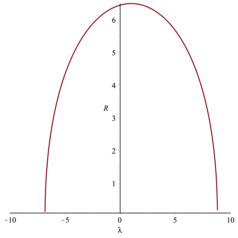
on the range of the areal radius. The latter begins from zero at , increases to the maximum
| (2.7) |
and then decreases until it vanishes again at . The two coordinate charts and cover the same physical region . We restrict ourselves to , in which , by choosing the negative sign in Eq. (2.5).
We write
| (2.8) |
and, substituting the relation between differentials
| (2.9) |
and using Eq. (2.8), the line element (2.1) becomes
| (2.10) |
The equation locating the apparent horizons (see, e.g., Faraoni:2015ula) has as the only root, which is a single root and therefore there are no apparent horizons for (we discuss the physical meaning of the formal root below).
The energy density Semiz:2020lxj
| (2.11) |
and the pressure (which are always non-zero) diverge at the origin , which corresponds to , together with the Ricci scalar
| (2.12) |
therefore there is a naked spacetime singularity at the origin .
The Misner-Sharp-Hernandez mass defined in spherical symmetry by MSH1; MSH2
| (2.13) |
reads
| (2.14) |
for the geometry (2.10) and is negative in the region around the naked singularity. This fact is not surprising: it has been argued that the Misner-Sharp-Hernandez mass (to which the Hawking-Hayward quasilocal mass Hawking; Hayward reduces in spherical symmetry Haywardspherical) is misbehaved near naked singularities, Cauchy horizons, or regions with the wrong asymptotic flatness Faraoni:2020stz; Faraoni:2020mdf. This is the case, for example, for the inner region of the Reissner-Nordström black hole near the Cauchy horizon, for the entire Schwarschild spacetime with negative mass, and for the Fisher-Janis–Newman–Winicour–Buchdahl–Wyman scalar field solution of the Einstein equations Fisher:1948yn; BergmannLeipnik57; Janis:1968zz; Buchdahl:1972sj; Wyman:1981bd; Dionysiu82; Agnese:1985xj; Virbhadra:1997ie for the parameter values for which there is a naked singularity Faraoni:2021nhi.
Let us come to the maximum value of the areal radius which, in spite of being a formal root of the equation , does not describe a horizon but is instead the antipode of the origin in a compact space. To see this fact, it is instructive to study the behaviour of radial null geodesics in this geometry. Consider the outgoing and ingoing congruences of radial null geodesics with tangents , where is an affine parameter along these curves. These tangents have components and the normalization yields
| (2.15) |
since a null vector can be rescaled by a function, we can choose (which means choosing the coordinate time as the affine parameter along these null geodesics), obtaining
| (2.16) |
We then have the first order equations
| (2.17) | |||
| (2.18) |
which integrate to
| (2.19) | |||
where is an integration constant. Unfortunately this relation cannot be inverted explicitly.
Since
| (2.21) |
(with the upper sign for outgoing and the lower one for ingoing radial geodesics), near the origin it is for outgoing and for ingoing geodesics. Furthermore, at . Outgoing radial null geodesics starting near the origin do so extremely fast but they slow down as they approach the maximum possible radius , which can only be reached with zero velocity (see Fig. 1). A null geodesic starting exactly at does so with zero velocity and remains there. Ingoing radial null geodesics starting near the maximum radius are slow and accelerate as they get closer to the central naked singularity, which they approach with infinite velocity .
We can also study radial timelike geodesics with tangents . The normalization gives
| (2.22) |
with the upper sign for outgoing and the lower one for ingoing geodesics. The timelike Killing vector guarantees the conservation of the energy per unit mass of the test particle along these geodesic curves:
| (2.23) |
where because these curves are future-oriented, hence is strictly positive. Equation (2.22) then gives
| (2.24) |
which tells us that:
- •
For a given energy determined by the initial condition , radial motion is only possible if
(2.25) (otherwise becomes imaginary). Ingoing radial motion stops at and a test particle cannot approach the origin, which is consistent with the fact that, according to Eq. (2.23), as .
- •
Outgoing radial motion stops at , where vanishes for both outgoing and ingoing radial geodesics, and a particle starting initially at remains there irrespective of its initial energy.
- •
Since is limited by , the possible energies are bounded from below,
(2.26) particles with energy below, or equal to, the minimum threshold do not move.
II.1 Case ,
In this case we are left with only two parameters . Now , which requires
| (2.27) |
The areal radius is
| (2.28) |
with corresponding to , while corresponds to the origin of the physical radial coordinate. The areal radius varies in the range
| (2.29) |
(where, in the last equality, we used the fact that ) and is a decreasing function of since is always negative in the allowed range. Inverting the relation between radial coordinates, one obtains
| (2.30) |
which, in conjunction with
| (2.31) |
yields the line element
| (2.32) |
This geometry is the same as that of the previous case , given by the line element (2.10), but now . Again, the energy density is non-zero and the Ricci scalar diverges at the origin .
II.2 Case
For these parameter values, requires to be positive and, therefore, we have the range of the Buchdahl radius. Correspondingly, the areal radius
| (2.33) |
varies in the interval
| (2.34) |
beginning from zero at , increasing to the maximum
| (2.35) |
and then decreasing until it vanishes again at . There are two coordinate charts and covering the same physical region and we restrict ourselves to the former, in which . Equation (2.33) yields
| (2.36) |
with roots
| (2.37) |
where we choose the lower sign for consistency with and . Then and
| (2.38) |
give the line element
| (2.39) |
which is the same as the line element (2.10), but with now given by Eq. (2.35). The Ricci scalar
| (2.40) |
diverges at the origin (which corresponds to in the chart with ), therefore there is a naked spacetime singularity there.
III General solution
The line element for the generic family of Semiz solutions is (1.3) Semiz:2020lxj. The presence of four parameters with relatively wide ranges now makes it difficult to reach definite conclusions and we focus on special cases.
III.1 is Schwarzschild
When , the energy density (1.5) and the pressure vanish identically and this spacetime is empty. Since the geometry is also spherically symmetric and asymptotically flat (as we are going to show) it must be the Schwarzschild one, according to the Jebsen-Birkhoff theorem Waldbook. In fact, we have , the areal radius is
| (3.1) |
and
| (3.2) |
then , yielding the line element
| (3.4) | |||||
where . This geometry is asymptotically flat: by introducing the constant
| (3.5) |
(which is not necessarily positive) and rescaling the time coordinate according to , the line element () is written as the Schwarzschild one
| (3.6) |
describing a black hole if and a naked central singularity if .
III.2 Special case
We have three parameters with and now ; the areal radius is
| (3.7) |
We have
| (3.8) |
which is positive for
| (3.9) |
To proceed, let us consider the situation , in which case increases in the interval
| (3.10) |
with and
| (3.11) | |||||
We have again a compact space. Rewriting the line element (1.3) in terms of the areal radius produces a cumbersome expression that does not depend only on but contains also because the relation cannot be inverted explicitly.
III.3 The even more special case
In this case we have only two parameters , , and the areal radius is
| (3.16) | |||||
where the last inequality follows from . Since
| (3.17) |
the areal radius is an increasing function of in the interval with , is maximum at and then decreases, vanishing again at . This compact space corresponds to the range
| (3.18) |
of the areal radius, with as . Equation (3.16) is inverted by first obtaining
| (3.19) |
and then solving for
| (3.20) |
where
| (3.21) |
while the two remaining roots are imaginary. Substituting the relation between differentials
| (3.22) |
and using
| (3.23) |
yield the line element
| (3.24) | |||||
where
| (3.25) | |||||
Again, the many combinations of parameters and the cumbersome metric coefficients do not lend themselves to a straightforward and transparent analysis, but it is clear that also in this case we have a compact 3-space of finite extent.
Using (3.20), the energy density (1.5) reduces to
as . Hence, and are singular at the origin, together with the Ricci scalar and
| (3.27) |
As , we have the asymptotics
| (3.28) | |||||
| (3.29) | |||||
| (3.30) | |||||
| (3.31) |
and while as .
IV Conclusions
We have studied the nature of the new classes of static and spherically symmetric solutions of the Einstein equations given recently in Ref. Semiz:2020lxj when the matter source is a perfect fluid with equation of state . The analytical solutions of Ref. Semiz:2020lxj that we analyzed (except for the Schwarzschild solution obtained for ) describe compact spaces with naked central singularities. The “general” family of solutions (1.3) and (1.5) always reduces to Schwarschild when the parameter vanishes. In most other situations, the presence of three or four parameters and/or the cubic nature of the function hamper a complete description of the geometry. However, in all cases analyzed, except for the empty spacetime associated with , we find a compact space of finite volume (a feature mentioned in Semiz:2020lxj).
The fact that the geometry, together with the energy density and the pressure, is singular at is not necessarily the death knell for these solutions. In fact, it is deemed acceptable for fluid solutions of the Einstein equations to only model limited regions of relativistic stars, a procedure that is reflected in the authoritative Ref. Stephani and in the more specialized literature. Indeed, even Newtonian stars are rarely modelled with a single fluid, corresponding to the fact that different regions at different temperatures and densities are described by different equations of state unless the stellar material is well mixed, which only happens in certain types of stars. Therefore, there is in principle the (physically well motivated) possibility of excising the singularity and replacing it with a more realistic geometry sourced by matter with a different equation of state. However, if one wants to describe a stellar interior with this exotic fluid, one must match it with an asymptotically flat Schwarzschild exterior. The fact that the solutions of Semiz:2020lxj describe compact spaces points to a possible analogy with the Oppenheimer-Snyder model of gravitational collapse to a black hole OppenheimerSnyder. In this model, a compact, positively curved Friedmann-Lemaître-Robertson-Walker universe collapsing to a Big Crunch is matched to a Schwarzschild exterior on the surface of a 2-sphere of symmetry OppenheimerSnyder, satisfying the Darmois-Israel junction conditions Darmois; Israel. However, in the Oppenheimer-Snyder model the matching is possible because the collapsing interior universe is filled by a dust with zero pressure everywhere. It is well known that the matching to a Schwarzschild exterior can only be done on a surface on which the pressure vanishes, otherwise the junction conditions are violated and there is a material layer on the matching surface, which is certainly not an ingredient of realistic stellar models. (This fact is highlighted in many studies of relativistic fluid balls Vaidyaball; MashhoonPartovi; SrivastavaPrasad; ThompsonWhitrow; ThompsonWhitrow2; Bondi; BondiNature; Faraoni:2020uuf and fireballs SmollerTemple.) However, for the fluid solutions of Semiz:2020lxj under discussion, the pressure never vanishes. Therefore, the best that one could do is modelling a limited region of a stellar interior with the Semiz solutions for . To be physical, this region should correspond to a positive Misner-Sharp-Hernandez mass and, therefore, should be sufficiently far away from the singularity at . The excised region containing the origin should be modelled with a different, non-singular, solution of the Einstein equations.11 1 There is a subtlety: matching a Semiz region with another fluid solution is in principle possible because the Semiz geometries solve the Einstein equations with zero cosmological constant . A non-zero would be present in all spacetime regions and matching one of them with a Schwarzschild exterior is impossible Faraoni:2021vpn. Then, the solution should be matched continuously with another “intermediate” solution with non-vanishing pressure on a surface of constant radius, and the pressure in this layer should then go to zero at larger radii to make it possible to match it to a Schwarzschild exterior, satisfying again the Darmois-Israel junction conditions. In the absence of a specific need for such an involved “star” model in astrophysics, we will not pursue this object further, limiting ourselves to pointing out the constraints for such a construction. Probably some of the phenomenology unveiled here for the geometries found in Semiz:2020lxj also applies to other classes of perfect fluid solutions of the Einstein equations. Whether this is the case will be established in future work.
Acknowledgements.
This work is supported, in part, by the Natural Sciences & Engineering Research Council of Canada (grant no. 2016-03803 to V.F.).References
- (1) İ. Semiz, “The general static spherical perfect fluid solution with EoS parameter ,” [arXiv:2007.08166 [gr-qc]].
- (2) A. DeBenedictis, R. Garattini and F. S. N. Lobo, “Phantom stars and topology change,” Phys. Rev. D 78, 104003 (2008) doi:10.1103/PhysRevD.78.104003 [arXiv:0808.0839 [gr-qc]].
- (3) G. Chapline, “Dark energy stars,” eConf C041213, 0205 (2004) [arXiv:astro-ph/0503200 [astro-ph]].
- (4) F. S. N. Lobo, “Stable dark energy stars,” Class. Quant. Grav. 23, 1525-1541 (2006) doi:10.1088/0264-9381/23/5/006 [arXiv:gr-qc/0508115 [gr-qc]].
- (5) N. Bilic, G. B. Tupper and R. D. Viollier, “Born-infeld phantom gravastars,” JCAP 02, 013 (2006) doi:10.1088/1475-7516/2006/02/013 [arXiv:astro-ph/0503427 [astro-ph]].
- (6) R. Chan, M. F. A. da Silva and J. F. Villas da Rocha, “Star Models with Dark Energy,” Gen. Relativ. Gravit. 41, 1835-1851 (2009) doi:10.1007/s10714-008-0755-9 [arXiv:0803.3064 [gr-qc]].
- (7) S. S. Yazadjiev, “Exact dark energy star solutions,” Phys. Rev. D 83, 127501 (2011) doi:10.1103/PhysRevD.83.127501 [arXiv:1104.1865 [gr-qc]].
- (8) F. Rahaman, R. Maulick, A. K. Yadav, S. Ray and R. Sharma, “Singularity-free dark energy star,” Gen. Relativ. Gravit. 44, 107-124 (2012) doi:10.1007/s10714-011-1262-y [arXiv:1102.1382 [gr-qc]].
- (9) D. Horvat and A. Marunović, “Dark energy-like stars from nonminimally coupled scalar field,” Class. Quant. Grav. 30, 145006 (2013) doi:10.1088/0264-9381/30/14/145006 [arXiv:1212.3781 [gr-qc]].
- (10) P. Bhar, “Dark energy stars in Tolman–Kuchowicz spacetime in the context of Einstein gravity”, Phys. Dark Univ. 34, 100879 (2021).
- (11) C. Armendariz-Picon and E. A. Lim, “Haloes of k-essence,” JCAP 08, 007 (2005) doi:10.1088/1475-7516/2005/08/007 [arXiv:astro-ph/0505207 [astro-ph]].
- (12) L. Amendola and S. Tsujikawa, Dark Energy: Theory and Observations (Cambridge University Press, Cambridge, UK, 2010).
- (13) H. Stephani, D. Kramer, M. MacCallum, C. Hoenselaers, E. Herlt, Exact Solutions of the Einstein Field Equations (Cambridge University Press, Cambridge, 2003).
- (14) M. S. R. Delgaty and K. Lake, “Physical acceptability of isolated, static, spherically symmetric, perfect fluid solutions of Einstein’s equations,” Comput. Phys. Commun. 115, 395-415 (1998) doi:10.1016/S0010-4655(98)00130-1 [arXiv:gr-qc/9809013 [gr-qc]].
- (15) R. M. Wald, General Relativity (Chicago University Press, Chicago, 1984).
- (16) V. Faraoni, Cosmological and Black Hole Apparent Horizons, Lect. Notes Phys. 907 (Springer, New York, 2015) doi:10.1007/978-3-319-19240-6
- (17) C. W. Misner and D. H. Sharp, “Relativistic Equations for Adiabatic, Spherically Symmetric Gravitational Collapse”, Phys. Rev. 136, B571 (1964).
- (18) W. C. Hernandez and C. W. Misner, “Observer time as a coordinate in relativistic spherical hydrodynamics”, Astrophys. J. 143, 452 (1966).
- (19) S. W. Hawking, “ Gravitational radiation in an expanding universe”, J. Math. Phys. 9, 598 (1968).
- (20) S. A. Hayward, “Quasilocal gravitational energy”, Phys. Rev. D 49, 831 (1994).
- (21) S. A. Hayward, “Gravitational energy in spherical symmetry”, Phys. Rev. D 53, 1938 (1996).
- (22) V. Faraoni and A. Giusti, “Unsettling physics in the quantum-corrected Schwarzschild black hole,” Symmetry 12, no.8, 1264 (2020) doi:10.3390/sym12081264 [arXiv:2006.12577 [gr-qc]].
- (23) V. Faraoni, A. Giusti and T. F. Bean, “Asymptotic flatness and Hawking quasilocal mass,” Phys. Rev. D 103, no.4, 044026 (2021) doi:10.1103/PhysRevD.103.044026 [arXiv:2010.00069 [gr-qc]].
- (24) I. Z. Fisher, “Scalar mesostatic field with regard for gravitational effects,” Zh. Eksp. Teor. Fiz. 18, 636-640 (1948) [arXiv:gr-qc/9911008 [gr-qc]].
- (25) O. Bergmann and R. Leipnik, “Space-time structure of a static spherically symmetric scalar field”, Phys. Rev. 107 (1957) 1157–1161, http: //dx.doi.org/10.1103/PhysRev.107.1157.
- (26) A. I. Janis, E. T. Newman and J. Winicour, “Reality of the Schwarzschild Singularity,” Phys. Rev. Lett. 20, 878-880 (1968) doi:10.1103/PhysRevLett.20.878
- (27) H. A. Buchdahl, “Static solutions of the Brans-Dicke equations,” Int. J. Theor. Phys. 6, 407-412 (1972) doi:10.1007/BF01258735
- (28) M. Wyman, “Static Spherically Symmetric Scalar Fields in General Relativity,” Phys. Rev. D 24, 839-841 (1981) doi:10.1103/PhysRevD.24.839
- (29) D. D. Dionysiou, “Static spherically-symmetric scalar-field theory in general relativity”, Astrophys. Space Sci. 88, 493 (1982).
- (30) A. G. Agnese and M. La Camera, “Gravitation without black holes”, Phys. Rev. D 31, 1280-1286 (1985) doi:10.1103/PhysRevD.31.1280
- (31) K. S. Virbhadra, “Janis-Newman-Winicour and Wyman solutions are the same,” Int. J. Mod. Phys. A 12, 4831-4836 (1997) doi:10.1142/S0217751X97002577 [arXiv:gr-qc/9701021 [gr-qc]].
- (32) V. Faraoni, A. Giusti and B. H. Fahim, “Spherical inhomogeneous solutions of Einstein and scalar–tensor gravity: A map of the land,” Phys. Rept. 925, 1-58 (2021) doi:10.1016/j.physrep.2021.04.003 [arXiv:2101.00266 [gr-qc]].
- (33) J. R. Oppenheimer and J. R. Snyder, “On continued gravitational contraction”, Phys. Rev. 56, 455 (1939).
- (34) G. Darmois, “Les Equations de la Gravitation Einsteinienne”, Memorial des Sciences Mathematiques XXV (Gauthier-Villars, Paris, 1927).
- (35) W. Israel, “Singular hypersurfaces and thin shells in general relativity”, Nuovo Cimento B 44, 1 (1966); Errata 48, 463(E) (1967).
- (36) P. C. Vaidya, “Nonstatic Analogs of Schwarzschild’s Interior Solution in General Relativity”, Phys. Rev. 174, 1615 (1968).
- (37) B. Mashhoon and M. H. Partovi, “On the gravitational motion of a fluid obeying an equation of state”, Ann. Phys. (NY) 130, 99 (1980).
- (38) D. C. Srivastava and S. S. Prasad, “Perfect Fluid Spheres in General Relativity”, Gen. Relativ. Gravit. 15, 65 (1983).
- (39) A. H. Thompson and W. J. Whitrow, “Time-Dependent Internal Solutions for Spherically Symmetrical Bodies in General Relativity: I. Adiabatic Collapse”, Mon. Not. R. Astron. Soc. 136, 207 (1967).
- (40) A. H. Thompson and W. J. Whitrow, “Time-Dependent Internal Solutions for Spherically Symmetrical Bodies in General Relativity: II. Adiabatic Radial Motions of Uniformly Dense Spheres”, Mon. Not. R. Astron. Soc. 139, 499 (1968).
- (41) H. Bondi, “Gravitational bounce in general relativity”, Mon. Not. R. Astron. Soc. 142, 333 (1969).
- (42) H. Bondi, “Bouncing Spheres in General Relativity”, Nature 215, 838 (1967).
- (43) V. Faraoni and F. Atieh, “Turning a Newtonian analogy for FLRW cosmology into a relativistic problem,” Phys. Rev. D 102, no.4, 044020 (2020) doi:10.1103/PhysRevD.102.044020 [arXiv:2006.07418 [gr-qc]].
- (44) J. Smoller and B. Temple, “Shock-wave solutions in closed form and the Oppenheimer-Snyder limit in General Relativity”, SIAM J. Appl. Math. 58, 15 (1998).
- (45) V. Faraoni, S. Jose and A. Leblanc, “Curious case of the Buchdahl-Land-Sultana-Wyman-Ibañez-Sanz spacetime,” Phys. Rev. D 105, no.2, 024030 (2022) doi:10.1103/PhysRevD.105.024030 [arXiv:2110.11289 [gr-qc]].