POSYDON: A General-Purpose Population Synthesis Code with Detailed Binary-Evolution SimulationsJournal: AAS JournalsThis manuscript has made use of the following Python modules: numpy (Harris et al. 2020), scipy (Virtanen et al. 2020), pandas (McKinney et al. 2010), matplotlib (Hunter 2007), astropy (Robitaille et al. 2013; Price-Whelan et al. 2018), scikit-learn (Pedregosa et al. 2011).
Abstract
Most massive stars are members of a binary or a higher-order stellar systems, where the presence of a binary companion can decisively alter their evolution via binary interactions. Interacting binaries are also important astrophysical laboratories for the study of compact objects. Binary population synthesis studies have been used extensively over the last two decades to interpret observations of compact-object binaries and to decipher the physical processes that lead to their formation. Here, we present POSYDON, a novel, publicly available, binary population synthesis code that incorporates full stellar-structure and binary-evolution modeling, using the MESA code, throughout the whole evolution of the binaries. The use of POSYDON enables the self-consistent treatment of physical processes in stellar and binary evolution, including: realistic mass-transfer calculations and assessment of stability, internal angular-momentum transport and tides, stellar core sizes, mass-transfer rates and orbital periods. This paper describes the detailed methodology and implementation of POSYDON, including the assumed physics of stellar- and binary-evolution, the extensive grids of detailed single- and binary-star models, the post-processing, classification and interpolation methods we developed for use with the grids, and the treatment of evolutionary phases that are not based on pre-calculated grids. The first version of POSYDON targets binaries with massive primary stars (potential progenitors of neutron stars or black holes) at solar metallicity.
I Introduction
Throughout their lives, stars affect their surroundings via the immense energy radiated across the electromagnetic spectrum (Conroy 2013; Eldridge & Stanway 2022, e.g.,) and the nuclear-processed material emitted as a stellar wind (Kudritzki & Puls 2000; Smith 2014, e.g.,). The deaths of massive () stars, even more than their lives, transform their environments as their cores run out of nuclear fuel and collapse to form neutron stars (NSs) and black holes (BHs). The formation of these compact objects (COs) is often accompanied by a supernova (SN) or a -ray burst that release more energy in than our Sun in (Janka 2012; Burrows & Vartanyan 2021; Woosley & Bloom 2006, e.g.,). These explosive events enrich their environments with heavier elements while also regulating any ongoing star-formation (Nomoto et al. 2013; Hopkins et al. 2011; Hopkins et al. 2012, e.g.,).
It is now established that most massive stars are members of a binary or a higher-order stellar system (Sana et al. 2013; Moe & Di Stefano 2017). More often than not, the presence of a binary companion decisively alters the evolution and final fate of both binary components via binary-interaction processes such as tidal dissipation, mass-transfer phases, and stellar mergers (Sana et al. 2012; De Marco & Izzard 2017). Furthermore, interacting binaries are arguably some of the most important astrophysical laboratories available for the study of COs. Accretion of matter from a binary companion gives rise to X-ray emission, bringing the system to the X-ray binary (XRB) phase (Bhattacharya & van den Heuvel 1991; Podsiadlowski et al. 1992), while gravitational waves (GWs) enable us to witness the last moments of the lives of coalescing binary COs (Abbott et al. 2016; Abbott et al. 2021).
Over the last two decades, multi-wavelength surveys of the Milky Way and its neighborhood, as well as numerous nearby and more distant galaxies, have amassed large datasets of binary stellar systems. These datasets range from targeted, high-resolution observations of galaxies in the local Universe (Dalcanton et al. 2012; Calzetti et al. 2015, e.g., the PHAT and LEGUS surveys;), to serendipitous (Evans et al. 2019, e.g., the Chandra Source Catalogue 2.0;), all-sky (Gaia Collaboration et al. 2018, e.g., Gaia;) and transient surveys (Kaiser et al. 2002; Graham et al. 2019, e.g., Pan-STARRS, Zwicky Transient Facility;). In addition to electromagnetic surveys, there is also the global GW observatory network of LIGO (Aasi et al. 2015), Virgo (Acernese et al. 2015) and KAGRA (Akutsu et al. 2019), which have detected nearly a hundred binary CO mergers (Abbott et al. 2021). Combined, these surveys are revolutionizing our view of binary stellar systems, including CO binaries, and their environments.
Aspects of the astrophysics of all these different types of stellar binaries can be obtained from observations and modeling of present-day properties of individual, well-studied systems. However, more comprehensive insight requires understanding the statistical properties of their entire populations. For these studies, binary population synthesis (BPS) modeling is often employed. BPS modeling first generates initial binary populations, whose properties are randomly sampled from probability distributions that can be observationally constrained. Then, this initial population is evolved with a computationally efficient simulation tool using our best understanding of the physics dictating binary star interactions, to produce observable properties of the target population. If the number of binaries evolved is large enough to provide a statistically significant description of a population of interest, then BPS can provide valuable insights about the expected rate and distribution of the target population’s properties, the different evolutionary pathways that lead to formation of these systems, and the effect that different physical processes have on their evolution.
Over the last two decades, many general purpose BPS codes have been developed, e.g., binary_c (Izzard et al. 2004; Izzard et al. 2006; Izzard et al. 2009), BPASS (Eldridge et al. 2017), the Brussels code (Vanbeveren et al. 1998a; Vanbeveren et al. 1998b), BSE (Hurley et al. 2002), ComBinE (Kruckow et al. 2018), COMPAS (Stevenson et al. 2017; Riley et al. 2022), COSMIC (Breivik et al. 2020), MOBSE (Giacobbo et al. 2018), the Scenario Machine (Lipunov et al. 1996; Lipunov et al. 2009), SEVN (Spera et al. 2015), SeBa (Portegies Zwart & Verbunt 1996; Toonen et al. 2012a), StarTrack (Belczynski et al. 2002; Belczynski et al. 2008), and TRES (Toonen et al. 2016). These have been used in studies of a wide variety of binary populations. A hard requirement for BPS is computational efficiency, as for most studies one would need to model the evolution of many millions of binaries in a reasonable computational time.
BPS codes stand in stark contrast to detailed stellar-structure and binary-evolution codes, e.g., BEC (Heger et al. 2000; Heger & Langer 2000), BINSTAR (Siess et al. 2013), the Cambridge STARS code (Eggleton 1971; Pols et al. 1995; Eldridge & Tout 2004; Stancliffe & Eldridge 2009), MESA (Paxton et al. 2015), and the TWIN code (Nelson & Eggleton 2001; Eggleton & Kiseleva-Eggleton 2002), which self-consistently solve the stellar structure equations of a binary’s component stars along with the orbital evolution. Many studies have used detailed binary-evolution calculations (Nelson & Eggleton 2001; Podsiadlowski et al. 2002; de Mink et al. 2007; Marchant et al. 2017; Qin et al. 2018; Qin et al. 2019; Langer et al. 2020; Misra et al. 2020; Laplace et al. 2020; Laplace et al. 2021, e.g.,) to generate grids of models, varying the masses of the two stars and the binary’s orbital period. However, in all those cases, the grids of detailed binary tracks either cover a limited part of the initial parameter space, or focus on a specific evolutionary phase. This limitation is principally caused by the computational demands of detailed grids; each simulation typically requires – CPU hours for the modeling of a single system (Paxton et al. 2019, e.g.,).
As a result of this computational expense, a common thread among the vast majority of current BPS codes is that they approximate each star’s evolution, employing either fitting formulae (Hurley et al. 2000, e.g., SSE;) or look-up tables (Kruckow et al. 2018, e.g., COMBINE;) for the properties of single stars, based on grids of pre-calculated detailed, single-star models. Then, the effects of binary interactions (e.g., Roche-lobe overflow or tides) are modeled using approximate prescriptions and parametrizations. This modeling approach is often called rapid or parametric BPS; throughout the remainder of this work, we choose to use the term parametric BPS (pBPS) modeling, to make a distinction between computational efficiency and modeling accuracy. A notable exception among BPS codes is BPASS (Eldridge et al. 2017), which uses extensive grids of detailed binary evolution models computed with a custom version of the Cambridge STARS binary evolution code (Stancliffe & Eldridge 2009). In the grids of binary-star models employed in BPASS, both the primary and the secondary stars are followed in detail, but only one at a time (for computational-cost reasons). During the primary’s evolution, the properties of the secondary star are approximated by formulae based on single-star models (Hurley et al. 2000). Subsequently, once the modeling of the primary’s evolution is completed, the secondary star’s evolution is re-computed, accounting for mass-transfer and rejuvenation effects.
Studies using pBPS techniques have allowed us to make advances in our understanding of the formation pathways leading to different types of binary systems, and to interpret observations of binary populations. Such examples are studies on white-dwarf binaries (Nelemans et al. 2001; Ruiter et al. 2009; Ruiter et al. 2010; Toonen et al. 2012b; Breivik et al. 2018; Korol et al. 2020, e.g.,), XRBs (Van Bever & Vanbeveren 2000; Belczynski et al. 2004; Fragos et al. 2008; Fragos et al. 2013b; Fragos et al. 2013a; Luo et al. 2012; Tzanavaris et al. 2013; Tremmel et al. 2013; Zuo et al. 2014; Zuo & Li 2014; van Haaften et al. 2015; Artale et al. 2019; Wiktorowicz et al. 2019; Shao & Li 2020, e.g.,), the Galactic population of double NSs (Osłowski et al. 2011; Andrews et al. 2015; Chruslinska et al. 2017; Vigna-Gómez et al. 2018; Chattopadhyay et al. 2020, DNSs; e.g.,), GW sources observable by ground-based observatories (Dominik et al. 2012; Dominik et al. 2013; Dominik et al. 2015; Mennekens & Vanbeveren 2014; Mennekens & Vanbeveren 2016; Belczynski et al. 2016; Klencki et al. 2018; Giacobbo et al. 2018; Mapelli & Giacobbo 2018; Neijssel et al. 2019; Spera et al. 2019; Kinugawa et al. 2020; Breivik et al. 2020; Zevin et al. 2020; Broekgaarden et al. 2021, e.g.,) and SNe in binary systems (De Donder & Vanbeveren 2003; Vanbeveren et al. 2013; Claeys et al. 2014; Zapartas et al. 2017; Zapartas et al. 2019; Zapartas et al. 2021, e.g.,).
However, the implicit assumption in pPBS codes that the binary components have properties identical to single stars of the same mass in thermal equilibrium (e.g., abundance profiles, core sizes, mass-radius relations and response to mass-loss), as well as the lack of information about the star’s internal structure at different critical evolutionary phases (e.g., the onset of a dynamically unstable mass-transfer, the end of stable and unstable mass-transfer phases or the core-collapse), may introduce systematic uncertainties and inaccuracies. Current pBPS codes therefore rely on approximate prescriptions for modeling binary interactions and difficult-to-calibrate additional model parameters. These complications could be avoided by instead employing detailed stellar-structure and binary-evolution simulations (hereafter detailed models). Focusing on aspects that are relevant to the formation of CO binaries, detailed models (i) allow for a self-consistent estimation of the mass-transfer rate, especially during thermal-timescale mass-transfer phases, and therefore an accurate assessment of mass-transfer stability; (ii) allow for a more accurate description of the type and properties of the formed CO as well as any potential associated transient events since the internal structure of pre-core-collapse stars is known, (iii) account for the transport of angular momentum between and within the binary components, including its back-reaction on the structure and evolution of each star (e.g., rotational mixing), and (iv) allow for the self-consistent modeling of the end of a mass transfer phase (e.g., accounting for a potential partial stripping of the envelope).
In this work, we build upon the combined experience gained from the large body of BPS studies to date, to create POSYDON (POpulation SYnthesis with Detailed binary-evolution simulatiONs), a general-purpose code that can generate entire populations of binaries, underpinned by detailed, self-consistent models of stellar binaries.11 1 POSYDON will become is publicly available at https://posydon.org upon publication of the paper . With POSYDON we aim to address many of the caveats of pBPS codes, while at the same time maintaining much of their flexibility. In its first release (v1.0), POSYDON is limited to stars of solar metallicity, and binaries where the primary star is massive enough to form a BH or a NS. Future releases, which are already in development, will lift these limitations. In Section II, we introduce POSYDON and the approach it takes to modeling binary populations. In Sections III and IV we provide the physics adopted for our detailed models of single and binary stars, respectively. We describe the pre-calculated grids of single and binary stellar evolution models in Section V, the way they are post-processed in Section VI, and our classification and interpolation methods for their optimal use in Section VII. In Section VIII we detail our treatment of evolutionary phases which are not based on pre-calculated grids, such as the core-collapse and the common-envelope (CE) phase, while in Section IX we describe how all the aforementioned pieces come together to model the entire evolution of a binary. In Section X we outline our assumptions and methods in modeling populations of binary systems and present some example results. We conclude in Section XI, where we present an outlook of future development directions of the POSYDON code. The definitions of all the symbols used throughout this paper can be found in Table I.
| Name | Description | First appears |
|---|---|---|
| Orbital separation | IV.1 | |
| Orbital separation before orbital kick | VIII.3.5 | |
| Orbital separation after orbital kick | VIII.3.5 | |
| Orbital separation pre common envelope | VIII.2 | |
| Orbital separation post common envelope | VIII.2 | |
| Rate of change of orbital separation | VIII.1.2 | |
| Rate of change of orbital separation due to wind mass loss | VIII.1.2 | |
| Rate of change of orbital separation due to tides | VIII.1.2 | |
| Rate of change of orbital separation due to gravitational-wave radiation | VIII.1.2 | |
| Non-dimensional spin | IV.2.3 | |
| Speed of light | IV.2.2 | |
| Depth of a convective region | VII.4 | |
| Orbital eccentricity | VIII.1.2 | |
| Orbital eccentricity after orbital kick | VIII.3.5 | |
| Rate of change of orbital eccentricity | VIII.1.2 | |
| Rate of change of orbital eccentricity due to tides | VIII.1.2 | |
| Rate of change of orbital eccentricity due to gravitational-wave radiation | VIII.1.2 | |
| Eccentric anomaly | VIII.3.5 | |
| Second-order tidal torque coefficient | IV.1 | |
| Dimensionless factor accounting for slow convective shells that cannot contribute to the tidal viscosity within an orbital timescale | IV.1 | |
| Fallback mass fraction | VIII.3.2 | |
| Convective exponential overshooting parameter | III.2.3 | |
| Local gravitational acceleration | III.2.1 | |
| Gravitational constant | III.2.2 | |
| Moment of inertia | IV.1 | |
| Moment of inertia rate of change | VIII.1.2 | |
| Specific angular momentum | V.7 | |
| Specific angular momentum of the ISCO | VIII.3.4 | |
| Angular momentum | V.7 | |
| Stellar shell’s angular momentum | VIII.3.4 | |
| Stellar shell’s angular momentum of directly collapsing material | VIII.3.4 | |
| Stellar shell’s angular momentum of disk forming material | VIII.3.4 | |
| Black hole angular momentum | VIII.3.4 | |
| Apsidal motion constant | IV.1 | |
| Star’s luminosity | III.2.2 | |
| Eddington luminosity | III.2.2 | |
| Second lagrange point | VIII.2 | |
| Mass of the initially more massive star | V.5 | |
| Mass of the initially less massive star | V.5 | |
| Mass of the accretor | IV.2.2 | |
| Mass of the donor | VIII.2 | |
| Mass of the compact object | V.6 | |
| Mass of the C/O core | VII.4 | |
| Mass of a convective region | IV.1 | |
| Mass of the binary companion star | IV.1 | |
| Mass of accretion disk | VIII.3.4 | |
| Mass of the stellar envelope | VII.4 | |
| Remnant’s gravitational mass | VIII.3.3 | |
| Mass of the He core | VII.4 | |
| Remnant’s baryonic mass | VII.4 | |
| Maximum neutron star mass | VIII.3.3 | |
| Mass-accretion rate corresponding to the Eddington limit | IV.2.2 | |
| Wind mass-loss rate | III.2.2 | |
| Binary stellar mass before core collapse | VIII.3.5 | |
| Binary stellar mass after core collapse | VIII.3.5 | |
| Stellar shell’s mass | VIII.3.4 | |
| Pressure | III.2.1 | |
| Orbital period | V.5 | |
| Binary mass ratio | IV.1 | |
| Stellar radius | III.2.2 | |
| Radius of the accretor | IV.2.2 | |
| Radial coordinate of a convective region’s bottom boundary | IV.1 | |
| Radius of the stellar core | VII.4 | |
| Radius of the C/O core | VII.4 | |
| Radius of the convective core | IV.1 | |
| Radial coordinate of a convective region’s center | VII.4 | |
| Radius of the donor | VIII.2 | |
| Radius of the He core | VII.4 | |
| Roche lobe radius | IV.2.2 | |
| Roche lobe radius of the accretor | IV.2.2 | |
| Radial coordinate of a convective region’s top boundary | IV.1 | |
| Stellar shell’s radius | VIII.3.4 | |
| Instantaneous orbital separation before orbital kick | VIII.3.5 | |
| Effective temperature | III.2.1 | |
| Timescale for orbital changes due to tides | IV.1 | |
| Magnitude of velocity kick | VIII.3.5 | |
| Orbital velocity of the collapsing star | VIII.3.5 | |
| Hydrogen mass function | IV.2.2 | |
| Center hydrogen mass function | VIII.1.1 | |
| Surface hydrogen mass function | VIII.1.1 | |
| Helium mass fraction | III.1 | |
| Center helium mass fraction | VIII.1.1 | |
| Surface helium mass fraction | VII.5 | |
| Metallicity (mass fraction of elements heavier than 4He) | III.1 | |
| Fraction of the orbital energy that contributes to the unbinding of the CE | VIII.2 | |
| Convective mixing length parameter | III.2.3 | |
| Thermohaline mixing parameter | III.2.3 | |
| Dimensionless factor denoting the radiative efficiency of the accretion process | IV.2.2 | |
| Stellar profile’s polar angle | VIII.3.4 | |
| Stellar profile’s polar angle of disk formation | VIII.3.4 | |
| Opacity | III.2.1 | |
| Parametrization of the CE’s binding energy | VIII.2 | |
| Optical depth | III.2.1 | |
| Tidal synchronization timescale | IV.1 | |
| Convective timescale | IV.1 | |
| Magnetic braking torque | VIII.1.2 | |
| Reduced mass | VIII.1.2 | |
| Maxwellian distribution dispersion | VIII.3.5 | |
| Maxwellian distribution dispersion for CCSN kicks | VIII.3.5 | |
| Maxwellian distribution dispersion for ECSN kicks | VIII.3.5 | |
| Binary orbital inclination with respect to before the kick | VIII.3.5 | |
| Surface angular velocity | III.2.2 | |
| Critical surface angular velocity | ||
| Orbital angular velocity | VIII.1.2 | |
| Stellar shell’s angular velocity | VIII.3.4 | |
| Stellar angular velocity | VIII.1.2 | |
| Stellar angular velocity rate of change | VIII.1.2 | |
| Stellar angular velocity rate of change due to winds | VIII.1.2 | |
| Stellar angular velocity rate of change due to changes of star’s moment of inertia | VIII.1.2 | |
| Stellar angular velocity rate of change due to tides | VIII.1.2 | |
| Stellar angular velocity rate of change due to magnetic breaking | VIII.1.2 III.2.2 | |
II Overview of the structure of POSYDON
At its core, a BPS code requires two elements: a method to generate random binaries at zero-age main sequence (ZAMS) and a mechanism to evolve those binaries. The former is described in Section X.1. Regarding the evolution of each binary, our primary goal with POSYDON is to self-consistently evolve the internal structures of the two stars comprising a binary along with the binary’s orbit. To achieve this goal, we have opted to employ the stellar-structure code Modules for Experiments in Stellar Astrophysics (Paxton et al. 2011; Paxton et al. 2013; Paxton et al. 2015; Paxton et al. 2018; Paxton et al. 2019, MESA;). However, calculating the evolutionary track of a binary using MESA can take in excess of CPU hours, a six-orders-of-magnitude increase in computational cost compared to a typical pBPS code such as COSMIC (Breivik et al. 2020). This means that, even with modern computing resources, we cannot feasibly run more than – binaries, far too few to accurately model a Milky Way sized population with stellar binaries. As a further complication, codes like MESA cannot run individual binaries from start to finish; key physics, including CE phases and supernovae require the code to be stopped and restarted.22 2 In principle these phases could be run within a stellar-structure code like MESA; for instance, more updated versions of MESA than the one we use can handle the evolution of a binary through a CE (Marchant et al. 2021).
POSYDON solves the problems associated with stellar-structure codes by using extensive, pre-calculated grids of single and binary stellar-evolution models, covering the parameter space relevant for the formation of high-mass binary stars, with separate grids being calculated for each phase of binary evolution. In v1.0 our grids contain a combined total of nearly 120,000 separate detailed binary simulations. To compute these grids, POSYDON has an infrastructure specifically designed for high-performance computing environments that streamlines the process of producing large grids with consistent physics inputs. Using this infrastructure, we have generated five separate grids of single and binary stellar evolution models. We computed three grids of interacting binary stars initially composed of two hydrogen (H)-rich ZAMS stars (Section V.5); a CO and a H-rich star at the onset of Roche-lobe overflow (RLO; Section V.6), and a helium (He)-rich ZAMS star with a CO companion (Section V.7). We further computed two grids of single H-rich and He-rich stars (Sections V.3 and V.4, respectively), which we use for the modeling of detached, non-interacting binaries. These five grids are then post-processed, so that their data size is reduced (Section VI). We additionally apply classification and interpolation algorithms on the outputs of these extensive grids (Section VII), allowing us to effectively interpolate between MESA simulations to estimate the evolution of any arbitrary binary within some bounded region of the parameter space. As a simpler alternative, we also provide functionality to evolve individual binaries using nearest-neighbor matching, and in that case no classification or interpolation methods are required.
The second major component of POSYDON is the code infrastructure to follow the entire evolution of a binary from start to end. To achieve this, we combined the aforementioned grids (and classification and interpolation methods) with physics dictating a binary’s evolution through key phases, including core collapse and CO formation (Section VIII.3) and CE (Section VIII.2). These latter phases are not modeled based on pre-calculated grids, but rather with on-the-fly calculations. Similarly, the evolution of detached, potentially eccentric, post-core-collapse binaries is also modeled with on-the-fly calculations, where we use the single-star grids coupled to binary evolution routines, i.e. orbital evolution due to tides, stellar winds, magnetic breaking and gravitational-wave emission (Section VIII.1).
In the POSYDON approach, each separate evolutionary phase (step) has its own dedicated function which determines the binary’s state resulting from that step, the quantitative values characterizing that binary (e.g., masses of the two stars), and the event describing how that state ended (e.g., onset of RLO). Once a step is completed, the POSYDON framework uses the resulting binary state and event as well as each component stars’ states to determine an individual binary’s next evolutionary step. The process is repeated until a binary’s evolution is complete, resulting in a disrupted binary, a binary merger, or a double CO. At this point, the next binary is run. The modular nature of POSYDON allows a user to also provide their own prescriptions to model each phase of evolution, or even their own breakdown of the binary-evolution tree. As default in POSYDON, we provide a complete set of evolutionary steps which we visually summarize in Figure 1 and present in detail in the following sections.
III Adopted stellar physics
All stellar-evolution models described in this paper were computed with the state-of-the-art, open source stellar-structure and evolution code MESA (Paxton et al. 2011; Paxton et al. 2013; Paxton et al. 2015; Paxton et al. 2018; Paxton et al. 2019) revision 11701 together with the 20190503 version of the MESA software development kit (Townsend 2020, SDK;).33 3 We made one minor bug fix in the MESA source code, which involves replacing the mass of the proton with the atomic mass unit where it appears in the code that evaluates the Potekhin & Chabrier 2010 equation of state (E. Bauer, 2020, private communication). This change is included in later MESA releases. MESA solves the one-dimensional stellar-structure and composition equations. Mixing and burning processes are solved simultaneously; mixing is treated as a diffusive process. Discussion of specific elements of stellar physics are described in the following subsections, which are split into microphysical and macrophysical processes. We implement all physics that are not readily available in MESA using the functionality provided by run_star_extras and run_binary_extras.
III.1 Microphysics
We adopt the Asplund et al. 2009 protosolar abundances as our initial composition, with and . The equation of state is the standard MESA amalgamation of the SCVH (Saumon et al. 1995), OPAL (Rogers & Nayfonov 2002), HELM (Timmes & Swesty 2000) and PC (Potekhin & Chabrier 2010) equations of state (Paxton et al. 2019). Radiative opacities are taken from Ferguson et al. 2005 and Iglesias & Rogers 1996 for the Asplund et al. 2009 mixture, along with electron conduction opacities from Cassisi et al. 2007. Nuclear reaction rates are drawn from the JINA Reaclib database (Cyburt et al. 2010). All models were computed using the approx21 nuclear reaction network that consists of 21 species: 1H, 3He, 4He, 12C, 14N, 16O, 20Ne, 24Mg, 28Si, 32S, 36Ar, 40Ca, 44Ti, 48Cr, 56Cr, 52Fe, 54Fe, 56Fe and 56Ni, plus protons and neutrons (for the purpose of photo-disintegration).
III.2 Macrophysics
III.2.1 Surface Boundary Conditions
The stellar surface boundary condition is satisfied by the simple_photosphere option, which sets the photosphere temperature using the Eddington 1926 relation, and the photosphere pressure via with enhancement due to radiation pressure at the photosphere (Paxton et al. 2011, e.g.,).
III.2.2 Stellar Winds
Stellar winds are a complex subject due to the varied physical mechanisms (known and unknown) that drive them and their dependence on the evolutionary state of their parent star. With this in mind, we have kept the wind prescription as simple as possible, while still capturing the key phenomenology of massive stellar evolution, but avoiding fine-tuning to reproduce any single subset of observations. In POSYDON, changing the wind prescription would require the computation of new set of single- and binary-star model grids.
For stars with initial masses above we use the MESA Dutch scheme, which consists of de Jager et al. 1988 for K and Vink et al. 2001 for K. In cases where K and the surface 1H mass fraction is below , the Vink et al. 2001 wind is replaced with the Wolf–Rayet wind of Nugis & Lamers 2000. Between 10,000 K and 11,000 K there is a linear ramp (as a function of ) between the two wind prescriptions. We do not explicitly include any luminous blue variable (LBV) type winds; however, our stellar models at solar metallicity (e.g., Figure 3) do not enter the regime where LBV-type winds are typically applied in other studies (Belczynski et al. 2010, e.g.,).
For stars with initial masses below , we again use the Dutch scheme for stars with hotter than 12,000 K. For stars with less than 8,000 K, we use the Reimers 1975 wind with scaling factor for stars on the first ascent of the giant branch, and the Bloecker 1995 wind with scaling factor for stars in the thermally-pulsating phase. For the case of 8,000 K 12,000 K, we calculate the wind for both the hot and cool schemes, and linearly interpolate between the two.
For mass-loss rates that have an explicit dependence on metallicity , we rescale wind mass loss based on the initial metallicity, not the current surface , as winds are driven predominantly by iron-group elements that remain almost constant throughout stellar evolution (Vink & de Koter 2005, e.g.,). The primary motivation for this approach is to avoid the dredge-up of carbon and oxygen to the surface layers in the later phases of evolution, which can cause surface to approach , from unduly influencing the mass-loss rate. The only exception here is the wind prescription by Nugis & Lamers 2000 for Wolf–Rayet stars, which is specifically calibrated to the total surface metal content, including carbon and oxygen: in this case, we use the current, surface value of the He-rich star.
We further boost stellar winds to limit a star’s rotation below its critical threshold , so that the sum of the centrifugal force and the photon pressure never exceeds gravity on the surface of the star. The impact of rotation on the mass loss rate is considered as indicated in (Heger & Langer 1998; Langer 1998),
| (1) |
where is the star’s wind mass-loss rate, and and are the angular velocity and critical angular velocity at the surface, respectively. The default value of the exponent is taken from Langer 1998. The critical angular velocity is given the expression , where is the Eddington luminosity and its expression is given in Eq. (8). This explicit boost to the wind is supplemented by an implicit numerical scheme implemented in MESA which ensures that the rotation of a star never exceeds its critical value.
III.2.3 Convection, Rotation, and Mixing Processes
Convective energy transport is modeled using mixing length theory (Böhm-Vitense 1958, MLT;) except in superadiabatic, radiation-dominated regions where we employ the MLT++ modifications introduced in MESA (Paxton et al. 2013) that reduce the superadiabaticity in radiation-dominated convective regions, to improve numerical convergence. For the condition of convective neutrality we use the Ledoux criterion, and we use the convective premixing scheme as described by Paxton et al. 2019. We adopt a solar-calibrated mixing length parameter, , based on results from the MIST project (Dotter et al., in preparation).
Rotation is implemented in MESA as described in Paxton et al. 2013; Paxton et al. 2019. Rotational mixing and angular-momentum transport follow the MIST project (Choi et al. 2016). It has been suggested that magnetic angular-momentum transport processes are main candidates for efficient coupling between the stellar core and its envelope during the post-MS (post-main sequence). Here, we adopt the Spruit–Tayler (ST) dynamo (Spruit 2002) that can be produced by differential rotation in the radiative layers and amplify a seed magnetic field. Stellar models with ST dynamo can reproduce the flat profile of the Sun (Eggenberger et al. 2005) and observations of the final spins of both white dwarfs and neutron stars (Heger et al. 2005; Suijs et al. 2008), but struggles to explain the slow rotation rates of cores in red giants (Eggenberger et al. 2012; Cantiello et al. 2014; Fuller et al. 2019).
MESA treats mixing processes in the diffusive approximation with MLT providing the basic description. In addition to MLT convection, we consider thermohaline mixing with the parameter (Paxton et al. 2013, Eq. 14), also referred to as (Charbonnel & Zahn 2007, Eq. 4), corresponding to an aspect ratio of the instability fingers (Kippenhahn et al. 1980). Thermohaline mixing is important during mass accretion from an evolved primary star onto an unevolved secondary star because the accreting material typically has a higher mean molecular weight than the material near the surface of the secondary star (Kippenhahn et al. 1980, e.g.,).
Overshoot mixing is treated in the exponential decay formalism (Herwig 2000; Paxton et al. 2011). For the parameter describing the extent of the overshoot mixing in this formalism, we adopt an initial-mass-dependent relation. For lower mass stars (initial masses less than 4 ) we adopt a value taken from the MIST project, , which is calibrated using the Sun, as well as open clusters (Choi et al. 2016). In the high-mass regime (initial masses greater than 8 ), we adopt a value of motivated by the work of Brott et al. 2011, who used the step overshoot formalism. Both of these values of are measured from a distance of the local pressure scale height into the convection zone from the formal convective-radiative boundary. This is the same approach adopted in the MIST models (Choi et al. 2016). In order to translate between the step and exponential-decay versions of overshoot mixing, we rely on the work of Claret & Torres 2017 which shows that the free parameter in the step formalism is a factor of larger than (their Figure 3). For stars with initial masses between and we smoothly ramp between the two values of . The mass range was chosen to be roughly consistent with the ranges considered in the two studies.
We include no extra mixing due to semiconvection (Langer et al. 1983, in the sense of ), as this process is implicitly accounted for in the convective premixing scheme (Paxton et al. 2019).
IV Adopted binary-star evolution physics
POSYDON is predominantly a BPS tool that simulates the evolution of an ensemble of binary systems through various stages of their life. In the POSYDON framework, we base the evolution of binary systems on three extended MESA binary grids, as shown in Figure 1. One grid consists of initially detached binary systems of two H-rich stars starting from ZAMS, where we follow the internal evolution of both stars with detailed models (Section V.5). A second grid consists of H-rich stars in a semi-detached system with a CO companion (Section V.6), and a third grid consisting of naked helium stars in an initially detached system with a CO companion (Section V.7). For the non-CO components in these binaries, we follow the same prescriptions for stellar structure and evolution as described in Section III. However, the internal structures of stars can be affected by the presence of a companion, principally through tidal interactions and mass transfer. In this section we describe how we use the binary module within MESA to model each binary’s orbit, while self-consistently accounting for the impact on each star’s structure.
IV.1 Tides
Tidal forces take place in binary systems, as each star tends to be deformed by the gravitational pull of its companion. Invoked by this gravitational deformation, frictional forces inside a star drive a binary toward circularization and stellar spin - orbit synchronization. In our MESA binary grids, we assume that the initial orbit is circularized and the stellar spins are synchronized with the orbit. This assumption should be valid especially for close orbits of massive stars, where tides are strong (Portegies Zwart & Verbunt 1996; Hurley et al. 2002). As binaries evolve, their orbital periods change as well as the individual stars’ rotation periods, potentially driving them out of synchronization. Therefore, it is only the process of spin-orbit coupling that is relevant for our grids of detailed binary-star models. In Section VIII.1 we discuss our treatment of eccentric, detached binaries.
We follow the linear approach to tides, which defines a timescale for synchronization (Hut 1981). In this approach, a torque is applied to non-degenerate stars in a binary corresponding to the difference between the orbital and the spin angular velocity , divided by the synchronization timescale :
| (2) |
where is the timestep and is the change in spin angular velocity over a particular timestep. Since every layer of a star rotates with its own angular frequency, Eq. (2) is separately applied to every layer. The torque applied to each layer of the star is added up and an opposite torque is applied to the binary’s orbit to ensure angular momentum conservation. Winds and mass transfer somewhat complicate the picture, and Paxton et al. 2015 gives a detailed description of how these effects are accounted for.
We separately calculate for both stars (Hut 1981; Hurley et al. 2002; Paxton et al. 2015):
| (3) |
Here , and are the mass, radius and moment of inertia of the star for which we calculate the tides, is the binary mass ratio, and is the orbital separation. is a dimensionless apsidal motion constant characterizing the central condensation of the star, and is the characteristic timescale for the orbital evolution due to tides. As Eq. (3) shows, is strongly dependent on the ratio of the stellar radius to the binary orbital separation. In practice, the quantity also varies significantly, depending on whether tidal dissipation occurs principally within convective regions (due to turbulent friction) or radiative regions (due to dynamical tides interacting with stellar oscillations). As stars may have both convective and radiative regions during their lives, at every timestep taken by MESA we separately calculate the dynamical and equilibrium tidal timescales, layer by layer, and apply the shorter of the two.
For radiative regions in a star, we calculate based on the dynamical tidal timescale from Zahn 1977, where
| (4) |
with as the second order tidal coefficient and the gravitational constant.44 4 This equation is equivalent to Eq. (42) of Hurley et al. 2002, apart from the typo correction of a square root, found in Sepinsky et al. 2007. For the calculation of , we adopt the latest prescriptions from Qin et al. 2018, who investigated the dependence of the parameter on the convective radius for various metallicities and evolutionary stages, finding
| (5) |
For the equilibrium tidal timescale, we calculate the synchronization timescale for each convective region in the stellar envelope using Eq. (3) and following Hurley et al. 2002:
| (6) |
and use the shortest timescale among them. In Eq. (6), is the mass of the convective region, is a non-dimensional numerical factor less than unity that takes into account slow convective shells that cannot contribute to the tidal viscosity within an orbital timescale, and is the convective timescale, which we take from Eq. (31) of Hurley et al. 2002, adapted to also accomodate convective regions that are below the surface:
| (7) | |||||
In the equation above, , , and are the radii of the top and bottom boundaries of the region, and the stellar luminosity respectively, in solar units. We use the surface luminosity in all calculations, as it is approximately constant throughout the envelope. Typically, the shortest equilibrium tidal timescale corresponds to the outermost convective region. In order to avoid tides being dominated by potential artificial convective shells that may appear during the numerical calculation of a star’s evolution, we only take into account regions that consist of at least consecutive shells in our models.

In Figure 2, we show two example evolutionary tracks in a Hertzsprung–Russell Diagram of the primary star in an interacting binary of and , for two different initial orbital periods ( days, top panel; days, bottom panel). We show which term of the tidal timescale dominates the tidal forces: the dynamical tidal timescale with orange, from Eq. (3) and Eq. (4), assuming the whole star is radiative, or the equilibrium tidal timescale with blue, from Eq. (3) and Eq. (6), according to the most important convective region of the star. We see that in the beginning of the evolution, the dynamical tidal timescale dominates, as expected for the MS of massive stars that have a radiative envelope. The day period system (top) initiates early RLO and does not form convective layers massive enough for equilibrium tides to dominate, until after the end of its MS. For the wider binary, even during the MS, the equilibrium tidal timescale tends to become comparable to the dynamical tidal timescale, due to convective regions that appear close to the surface of the star. These regions include a small part of the total mass of the star (as low as ), but have a significant radial thickness. The equilibrium tidal timescale dominates in all the remaining parts of the evolution, apart from the He core burning phase of the stripped primary in the 3 days period system.
IV.2 Mass-transfer
Over the course of a binary’s evolution, the outermost layers of one of the binary’s stellar components may be removed, due to the gravitational pull of its companion. As a consequence of either the binary’s orbit decay or the expansion of a star’s envelope, this transfer of mass is dictated by the geometry of the Roche potential, namely the gravitational potential constructed in the co-rotating reference frame of the binary system.
IV.2.1 Mass Loss Rates from a Star Overflowing its Roche Lobe
To calculate mass-loss rates (due to mass transfer only) from main-sequence (MS) stars that overfill their Roche lobes, we use the contact scheme within MESA. This prescription is a numerical approximation; for stars overfilling their Roche lobes at the beginning of each timestep, mass is removed such that by the end of the timestep, the star remains confined to within its Roche lobe. For MS stars, this approximation is consistent with more accurate methods, as MS stars are compact, with relatively small pressure scale heights. We choose this prescription, as it allows us to evolve binary systems in which both stars overfill their Roche lobes simultaneously (Marchant et al. 2016).
As stars evolve off the MS, however, they tend to expand, forming less dense envelopes as they become giant stars. The large pressure scale heights of giant stars cause the contact scheme to become inaccurate, and a prescription is required that can more accurately treat these stars’ extended envelopes. For stars with a central H abundance less than , we switch to the Kolb scheme (Kolb & Ritter 1990).55 5 The current version of MESA does not allow the reversing of the donor star in this scheme. Occasionally, an once accreting star evolves off the MS, expands, and itself overfills its Roche lobe. In these cases mass transfer is not calculated, and the system predominantly leads to L2 overflow. This prescription allows the star to expand beyond its Roche lobe, and self-consistently calculates the rate that mass can flow through the inner Lagrangian point based on the local fluid conditions.
IV.2.2 Mass Accretion onto a Non-Degenerate Companion
The evolution of a binary during a mass transfer phase depends not only on the mass-losing star but also on the mass-gaining star. Based on the nature of the accretor, the process of accretion is treated differently.
For binaries with a non-degenerate accretor (those in our grid of two H-rich stars), initially all the mass lost by the donor through RLO is accepted by the accretor. We assume that material being accreted carries the specific angular momentum according to de Mink et al. 2013. This prescription allows for the distinct treatment of accretion via direct impact of the incoming stream on the stellar surface, or, in case of accretion onto a more compact star, the formation of a Keplerian disk around the accretor. The accreted angular momentum spins up the accretor, and mass accretion is restricted when the accretor reaches critical rotation. Mass falling within a critically rotating accretor’s gravitational potential will be ejected from the binary with the specific angular momentum of the accretor (Paxton et al. 2015) in the form of rotationally-enhanced stellar winds, following Eq. (1). At the same time that accretion is spinning up the outer layers of a non-degenerate star, internal mixing processes transport the surface angular momentum toward deeper layers, slowing the star’s rotation rate.
IV.2.3 Accretion onto a Degenerate Companion
Mass transfer onto a degenerate star proceeds similarly as that onto a non-degenerate star, with a few notable exceptions. The primary exception is that mass transfer is capped at the Eddington limited rate. For sub-Eddington mass-transfer rates onto a CO, mass transfer is assumed to be conservative. However, for super-Eddington rates, the excess matter is lost from the vicinity of the accretor as an isotropic wind (i.e., with the specific angular momentum of the accretor).
We calculate the Eddington-limited rate using standard formulae (Frank et al. 2002). We first calculate the Eddington luminosity for an accretor with mass :
| (8) |
where is the opacity of the incoming material and is the speed of light. For a fully ionized gas, Thompson scattering dominates the opacity, so , where is the hydrogen abundance of the donor. By setting equal to the radiation released by accreted matter as it falls into a CO’s potential well (), we can recover the Eddington-limited accretion rate,
| (9) |
The dimensionless constant sets how efficiently the rest mass energy of the incoming matter is converted to outgoing radiation,
| (10) |
For BHs, is set by the spin-dependent innermost stable circular orbit, while for NSs, we use a constant of km (Most et al. 2018; Miller et al. 2019; Riley et al. 2019; Landry et al. 2020; Abbott et al. 2020a; Kim et al. 2021; Biswas 2021; Raaijmakers et al. 2021). Our grids containing a CO components, are currently focused on NS and BH accretors, for which we simulate a range of masses. The type of a CO is determined solely on its mass, with COs having gravitational mass less than being classified as NSs, while those with mass greater than as BHs. Within our code, the only difference between these types of accretors is the corresponding ; otherwise accretion proceeds identically regardless of the type of CO accretor.
As these COs accrete material, they ought to accrete angular momentum. In our current version of the grids, we ignore any corresponding increase in the spin rate of NSs. For BHs, on the other hand, we self-consistently incorporate the increase in spin frequency as well as its effect on through the radius of innermost stable circular orbit (Podsiadlowski et al. 2003, ISCO;),
| (11) |
where is the initial mass of the accreting BH and its current one. In this equation it is also implicitly assumed that the birth spin of the BH is 0, as it has been suggested by several studies (Fragos & McClintock 2015; Qin et al. 2018; Fuller & Ma 2019). The corresponding increase in the BH’s non-dimensional spin rate, , can be calculated following Thorne 1974 and King & Kolb 1999,
| (12) |
These equations both assume that the spin-up occurs due to angular momentum accretion from a disk that is truncated at the ISCO.
We do not explicitly stop our simulations if a NS accretes enough mass to cross our 2.5 threshold thereby collapsing into a BH, but we do switch the instantaneously.
IV.2.4 Onset of CE
Stars with radiative envelopes entering RLO respond to mass loss by shrinking (Hjellming & Webbink 1987); mass transfer then reaches a natural equilibrium set by the strength of some driving force (nuclear evolution, tides, thermal expansion or some other effect), and how quickly the orbital separation, and thus the Roche lobe radius, change due to mass transfer through the inner Lagrangian point. However, in certain circumstances mass transfer increases in a runaway process, either because stars expand due to mass loss (e.g., stars with deep convective envelopes) or because the binary’s orbit shrinks faster than a donor star’s radius (Paczyński & Sienkiewicz 1972, e.g.,). These phases of binary evolution are notoriously difficult to model as they are intrinsically three-dimensional processes, and they span many orders of magnitude in spatial and temporal scales (Ivanova et al. 2013). We therefore stop our MESA models when binaries enter dynamically unstable mass transfer; we provide a description of how we address this phase in Section VIII.2. Here we focus on the conditions we use to identify when a binary enters dynamically unstable mass transfer.
First, we assume that a dynamically unstable RLO phase is initiated whenever mass-transfer rate exceeds yr-1. It is expected that binaries reaching this limit will only further increase their mass-transfer rates, as this corresponds to a dynamical limit on the mass-loss rate for giant stars (with dynamical timescales of years). As a check, we carried out a calibration test where we followed the evolution of a test binary to mass transfer rates even larger than yr-1. In every test we ran, we found that the mass-transfer rate increases to arbitrarily high rates, confirming the validity of our limit. Assigning a limit to the mass-transfer rate also avoids numerical issues caused by the effort of stellar models to converge with such extreme mass loss.
As a second condition, we assume dynamically unstable RLO occurs when the stellar radius of the expanding star extends beyond the gravitational equipotential surface, passing through the second Lagrangian point (L2). In such cases the lost matter from the L2 point carries substantial angular momentum, rapidly shrinking the orbit and leading to a runaway process in which the two stars spiral in and trigger a CE (Tylenda et al. 2011; Nandez et al. 2014). We use the prescription from Misra et al. 2020 to define the spherical-equivalent radius corresponding to L2. This condition cannot occur for MS donors, since the contact scheme for RLO forces a star’s radius to be contained within its Roche lobe. For cases where two MS stars overfill both their Roche lobes, in an over-contact binary, we alternatively use the prescription from Marchant et al. 2016 for the L2 radius, which considers that both stars can contribute to the overflow of the L2 volume together.
| Initial state | Parameters’ range and resolution | |||||||||||
|---|---|---|---|---|---|---|---|---|---|---|---|---|
| Star 1 | Star 2 | aaTotal number of models in this grid. | Failures bbPercentage of models that stopped due to numerical-convergence errors before reaching one of our stopping conditions. These rates describe the finalized grids, after a series of re-runs have occurred; see Section VI.1 for details. | |||||||||
| ZAMS | - | 0.5–300 | 0.014 | - | - | - | - | - | - | 200 | 1.5% | |
| ZAHeMSccZero-age He Main Sequence stars. | - | 0.5–80 | 0.055 | - | - | - | - | - | - | 40 | 0% | |
| ZAMS | ZAMS | 7 6.2–120 | 0.025 | - | - | 0.05–0.95 | 0.05 | 0.72–6105 | 0.07 | 56000 58240 | 0.9 1.5% | |
| Evolved, H-rich ddAlthough this grid is initialized with H-rich stars at ZAMS, we ignore the portion of each simulated binary’s evolution prior to the onset of RLO. The initial state of Star 1 in this grid are therefore somewhat evolved. | CO | 0.5–120 | 0.06 | 1–35.88 | 0.074 | - | - | 1.26-3162 | 0.13 | 25200 | 0.8 0.9% | |
| ZAHeMS | CO | 0.5–80 | 0.055 | 1–35.88 | 0.074 | - | - | 0.02–1117.2 | 0.09 | 39480 | 4.7 4.8% | |
For CO accretors, we set a third condition for unstable mass transfer based on the photon trapping radius (Begelman 1979; King & Begelman 1999). Inside that radius photons are advected inward along with accreted matter onto the accretor, while outside that radius, photons diffuse away. For stable mass accretion, the photon trapping radius occurs close to the accretor; however, as the accretion rate increases, the photon trapping radius expands. Once the photon trapping radius reaches the Roche-lobe radius of the accretor it is assumed to lead to a CE phase. Since the radius of the photon trapping envelope depends on the Eddington limit of the accretor and the mass-transfer rate from the donor , we limit the latter assuming an instability condition when (Begelman 1979):
| (13) |
As a final condition, occasionally two stars will both overfill their Roche lobe while one of those stars has evolved off the MS. Since the contact scheme in MESA can only evolve binaries in which both stars are on the MS, we assume these binaries automatically enter a CE.
As a test we compared the first three dynamical instability conditions separately to investigate their effect and found that the limiting mass accretion rates are all similar: as soon as a binary reaches any one of them, the other two are close to their limits as well. Therefore, for a particular binary in our MESA simulation, the binary is considered to enter a CE if any one of them occurs.
V Grids of detailed single- and binary-star evolution models
While in Section III and Section IV we describe the physics we adopt in our simulations, here we provide numerical details about how we produce each of our five MESA grids. This includes our procedure for producing initial stellar models for each of our grids (Section V.1), our termination conditions common across all of our grids (Section V.2), and a description for each of our five grids of binary simulations (Sections V.3–V.7). We summarize the basic properties of each grid in Table 2.
V.1 Zero Age Main Sequence Models
We create our own library of ZAMS models for both H-rich and He-rich stars. For the creation of the H-rich ZAMS models we use the MESA revision 11701 template create_zams. The process begins with creating a fully-convective star with no nuclear fusion taking place and adopting our protosolar abundances (Section III.1). This model is then evolved with our adopted nuclear reaction network until the H-burning luminosity exceeds 99% of the total luminosity.
The He-rich ZAMS (ZAHeMS) models are created in three steps. First, we create a pre-MS He star with 100% 4He in the same way that we create a H-rich pre-MS star. In the second step we adjust the initial metallicity. In the third step we evolve the model until the He-burning luminosity exceeds 99% of the total luminosity.
The two sets of ZAMS and ZAHeMS models are used as a starting point for the five grids of single- and binary-star models.
V.2 Termination conditions
We set conditions for the termination of our evolutionary models based on both single-star properties and binary-star properties. If any one of these conditions are met by an individual simulation, it is terminated at that timestep. Our termination conditions are:
- •
A star’s age exceeds the age of the Universe (13.8 Gyr), a condition that is typically only met for the lowest-mass stars we simulate (). In our single-star grids, for numerical purposes, we allow stars to evolve beyond this condition, then truncate their evolution afterwards at the end of the MS, which may extend beyond the age of the Universe.
- •
A star becomes a WD, a condition we quantify by checking if the central degeneracy parameter (Coulomb coupling parameter) exceeds 10 (Choi et al. 2016).
- •
A star reaches the end of core C-burning, a condition triggered when the fractional abundances of both C and He decrease below and , respectively, at the star’s center.
- •
A binary enters a CE phase, as described in Section VIII.2.
- •
A star reaches the thermally-pulsating asymptotic giant branch (TP-AGB) phase and then reaches a point of failure (numerical non-convergence) during thermal pulsations. Because these are not uncommon and we consider the nascent WD to be well-formed be within the AGB star, we consider this evolution to be successful.
Our simulations may occasionally end prematurely before any of the aforementioned conditions are reached. This may happen because the minimum timestep limit within MESA ( s) is reached or any individual simulation reaches our maximum runtime on our computing cluster (set to 48 hours). We provide details describing how we approach such runs in Section VI.1, but these failures are rare, occurring a few percent or less in each grid.
V.3 H-rich, single-star grid
Our first grid of single-star evolutionary models contains a series of non-rotating H-stars with our adopted protosolar composition of and . The grid consists of 200 masses, ranging from to with a logarithmic spacing of dex. For each star, models were initialized using the procedure described in Section V.1, and evolved until one of the termination conditions provided in Section V.2 occurs.
To test their validity, we compare POSYDON evolutionary tracks to the widely used stellar evolution tracks from the Geneva (Ekström et al. 2012, upper panel;), MIST library (Choi et al. 2016, center panel;), and BSE as implemented in COSMIC (Pols et al. 1998; Hurley et al. 2000; Breivik et al. 2020, lower panel;) groups in Figure 3. In all cases we show non-rotating models with initial masses between 1 and 300 . The pre-MS evolution is omitted from the MIST evolutionary tracks and the TP-AGB and post-AGB phases are omitted for clarity. All sets of tracks show a similar location for the ZAMS; the subsequent evolution along the MS and through He-burning phases differs due to the way each set of models treats mixing across convective boundaries. The clearest differences between the POSYDON and other models are in the location of the hook feature near the MS turnoff for higher masses, a result of the different adopted core overshoot treatments, and the positions of later phases, a result of the different wind mass-loss treatments among the different groups. The COSMIC tracks extend to larger radii and cooler effective temperatures, which may place them in the regime of LBVs; however, none of the other sets of evolutionary tracks enter this regime. For a more in depth comparison see, e.g., Agrawal et al. 2020; Agrawal et al. 2022.
.
Figure 4 compares the final C/O core mass between POSYDON, MIST, and SSE as implemented by COSMIC. SSE models are calculated until central C-burning, while MIST and POSYDON are calculated through central C-exhaustion for those stars with sufficient mass to ignite carbon or to the WD cooling sequence for lower masses. Differences between the core masses of MIST and POSYDON are generally due to the different overshooting parameter (we adopt for stars with masses above 8 , compared with adopted by MIST). The COSMIC/SSE models exhibit different behavior at larger masses as these prescriptions are based on stellar models that only go up to 50 ; larger masses than this are an extrapolation.

V.4 He-rich, single-star grid
Our second grid of single-star evolutionary models consists of non-rotating He-rich stars with and our adopted protosolar . This grid consists of 40 masses ranging from to with a logarithmic spacing of dex. For these masses, stellar evolution models were computed starting from ZAHeMS models (Section V.1) and evolved until one of the termination conditions described in Section V.2 occurs. For all but the lowest-mass cases, the core C depletion condition is the relevant one; models with initial masses below do not ignite C-burning in the core, and therefore terminate as He-core WDs.
As a test of our POSYDON He-star models, we compare their lifetimes to those of the He-star models of Woosley 2019 in Figure 6. Only the overlapping range of initial masses is shown here; the Woosley 2019 grid includes models with masses from 1.8–120 . These models match to within dex in log lifetime across the entire range of initial masses.
As a second test, we compare the final masses between the same two model grids in Figure 7. Although the lifetimes are similar, the final masses show a significant difference, particularly at higher initial He-star masses. Woosley 2019 notes that the change in slope of the initial-final mass relation around of 11 is due to the mass-loss prescription adopted for exposed CO cores; at larger initial He-star masses, the entire He-star mass is burned to heavier elements. For all the single- and binary-star model grids in POSYDON, we adopt the mass-loss prescription from Nugis & Lamers 2000 for He-rich stars. The latter predicts on average stronger wind mass loss than the prescription from Yoon 2017 adopted by Woosley 2019, leading to the substantially different final masses between the two prescriptions at .
Finally, we show the radius evolution of the He star tracks for the mass interval of 2–10 in Figure 8. He-rich stars exhibit a peculiar feature where less-massive stars expand farther on the giant branch than their more massive counterparts, in agreement with results by Habets 1986. When in a binary system, this implies that there is a relatively narrow range of orbital periods in which massive He stars will undergo RLO. Less massive He stars expand to hundreds of , leading to a wide range of orbital periods in which these stars can interact with a putative companion. This behavior is realized in our binary star grids, and its effects are seen explicitly in Figure 14.
V.5 Binaries consisting of two hydrogen-rich main-sequence stars


For modeling the evolution of two ZAMS stars in a binary system, we run a grid of 58,240 separate binary evolution models, varying the initial mass of the primary star , the initial binary mass ratio (where is the mass of the companion star), and orbital period . We consider values of initial primary masses, ranging from to with a logarithmic spacing of dex, and values of initial binary mass ratios, ranging from to with a spacing of . Finally, we cover values of initial orbital period, ranging from days to days with a logarithmic spacing of dex, in order to explore all binary configurations ranging from close systems in initial RLO to wide systems that never exchange any mass.
We simulate binaries by first separately initializing two H-rich, single stars at ZAMS following the procedure defined in Section V.1. We then place those stars in a binary with a second relaxation step, where we force their their rotation periods to be synchronized with the orbital period, implicitly assuming that the synchronization has happened during the pre-MS phase. The latter might not be true for wide binaries, but our assumption induces negligible rotation to the stellar components of those systems and does not affect their further evolution. As long as both stars in the binary are under-filling their Roche lobes after this relaxation step, we start to evolve the binary. Evolution continues until one of the termination conditions described in Section V.2 occurs.
In Figure 9 we provide two two-dimensional slices of this grid, where we show our simulation outcomes as a function of and for fixed values. In the left panel we show one example of a mass ratio , and on the right a more-equal mass slice. Each point in the panels represents a separate simulation from our grid. Diamond markers represent models that terminated in a CE, while square markers represent models that terminated when one of the stars completed its evolution (e.g., reached core C exhaustion). These are systems that experienced either only stable mass-transfer episodes or no mass transfer at all, so their evolution can be continuously modeled. At the bottom of each panel we see systems that are born filling their Roche lobes (black dots). These systems are assumed to merge, and therefore never produce a viable binary. Finally, a small fraction of systems never complete their evolution, producing binary stellar models that at some point fail to converge (red diamonds).
Separately, the color of each marker indicates that particular binary’s mass transfer history. Systems with sufficiently close initial tend to lead to contact phases (orange) where both stars fill their Roche lobes simultaneously. Most, but not all, of these system end up entering a CE phase. Sufficiently widely separated (or very massive) systems never fill their Roche lobes, and therefore never interact (gray markers). For intermediate orbital periods, the colors differentiate the evolutionary state of the donor when the latest mass transfer phase was initiated, ranging from MS (blue) to post-MS (tan), to stripped He-MS (brown). Stable mass transfer causes the donor star to be almost completely stripped of its H-rich envelope. In the latter case (brown) the low-mass stripped donors initiate a second mass transfer phase (Case BB mass-transfer) when they re-expand (Delgado & Thomas 1981; Laplace et al. 2020).


Comparison between the two panels shows that the mass ratio leads to a stark difference in the mass-transfer outcomes. Whereas nearly all systems with an initial result in stable mass transfer, the opposite is true for our systems. At the same time, some features between the two mass ratios are similar: (i) The boundary between interacting and non-interacting systems seems to be insensitive to (and therefore the secondary’s mass). At the largest orbital periods, stars do not expand far enough to overfill their Roche lobes. At the largest masses, stars have extremely strong winds that widen their orbits, simultaneously stripping the primary of its H-rich envelope, and these stars never expand enough to fill their Roche lobes. (ii) Systems with initial days tend to result in dynamically unstable mass transfer. (iii) There is a large region of binaries with initial primary mass 40–50 that stably overfill their Roche lobes as post-MS stars. These stars achieve their mass transfer stability mainly due to their strong stellar winds, which increases the mass ratio and the orbit of the system until the moment of overflow.
We model, and keep track of, the properties of both stars in the binary system throughout their evolution, as well as their detailed internal structure at the end of the models. In Figure 10 we show, for the same two mass-ratio slices as in Figure 9, the final rotational rate of the secondary (the initially less massive) stars for systems that avoid dynamically unstable mass transfer. Each marker’s color is set by how close each star’s rotation rate is to its critical rate. Highly rotating secondary stars have all experienced substantial mass and angular-momentum accretion during their evolution. Many of them have reached critical rotation, , early during mass transfer, at which point further mass accretion becomes non-conservative (c.f. Section IV.2.2). The right-hand panel shows that the companion’s rotation rate is closely linked with , as companion stars with lower mass primary stars also have lower masses and therefore do not lose as much angular momentum through their own stellar winds. This behavior is independent of the assumed initial rotation of the stars.
We find a small subset of initially very close systems in the bottom right corner (log and log) that retain a significant rotational rate even though they avoid mass transfer. In binaries with such tight orbits, tidal forces between the stars are sufficiently strong to keep them fast rotating, despite their strong winds.
V.6 Binaries consisting of a compact object and a hydrogen-rich star, at the onset of Roche-lobe overflow


Our second grid of binary star simulations consists of a H-rich star in a binary with a CO at the onset of RLO. This grid consists of 25,200 binary evolution models, where we vary the initial mass of the primary star , the initial mass of the CO , and the orbital period . We consider values of initial primary masses, ranging from to with a logarithmic spacing of dex, and values of initial CO masses, ranging from to with a logarithmic spacing of dex. Finally, we cover values of initial orbital period, ranging from days to days with a logarithmic spacing of dex. Our choice of CO mass range covers massive WD, NS, and BH accretors.
Our procedure in constructing this grid is different from what was described in Section V.5. We start each of the simulations with binaries composed of a ZAMS H-rich star and a CO, which in the MESA code is approximated by a point mass. Initially, and until each of the binary models reach the onset of RLO, we neglect orbital angular-momentum loss mechanisms, such as tides, magnetic breaking and gravitational radiation, while we artificially enforce the synchronization of the non-degenerate star with the orbit at all times. We do, however, allow for wind mass-loss from the non-degenerate star, which also results to a widening of the orbit. Once the onset of RLO is reached, we include the effects of all orbital angular-momentum loss mechanisms and discard the prior evolution of the system, treating the onset of RLO as the effective starting point of our models. Furthermore, from that point onward, we do not artificially enforce the synchronization of the non-degenerate star’s spin rotation with the orbit, but we instead follow the tidal synchronization process self-consistently, following the prescriptions described in Section IV.1. Finally, binaries that never reach the onset of RLO are not considered further; these detached binaries are modeled separately as described in Section VIII.1. There, we also provide a full explanation of how we use this binary-star grid, composed of a H-rich star and a CO at the onset of RLO, within a larger infrastructure to completely evolve binaries from ZAMS to double COs.
Figure 11 shows two slices of the grid with different CO masses, M⊙ to represent a NS accretor and M⊙ to represent a more-massive BH accretor. The symbols depicted in Fig. 11 have the same meaning as in Figure 9. Although our true initial binary parameters are regularly spaced, and on the axes shown in Figure 11 are the binary’s quantities at the onset of RLO, the effective starting point of the models; therefore, the grid does not appear to be regularly spaced (strong winds exhibited by massive stars tend to expand binary orbits prior to mass transfer). We do not show those binaries that never interact (even though we ran these simulations). As already seen in the binary-star model grid composed of two H-rich stars (Figure 9), binaries too widely separated will never overfill their Roche lobes, and binaries with massive H-rich stars have winds too strong to expand into giant phases. In this grid, Figure 11 shows an additional region of white space at low mass ( ) that occurs because these stars remain on the MS for the entirety of the simulation, never expanding to fill their Roche lobes within the age of the Universe.
Examining the stability of the mass-transfer phase, Figure 11 shows that nearly every donor star accreting onto a M⊙ BH does so stably, whereas only the lower mass accretors (4.5 ) do so for NS accretors. This difference is because the stability of a mass transfer in a binary primarily depends on the mass ratio, with a higher accretor mass allowing for higher donor masses. Our findings, at least for the case of NSs, are consistent with recent results from Misra et al. 2020, who use the same criteria to define the onset of L2 overflow leading to dynamical instability as done in our work.


Figure 12 shows the relative changes in the accretor masses in the same two slices in as Figure 14. High amounts of accretion mainly depends on two factors: a sufficiently high-mass accretion rate and a long-lasting RLO phase. In both panels, this happens for binaries with short periods day, and pre-RLO mass ratios in the range – (defining ). Despite our assumption of Eddington-limited accretion, for these binaries, stable accretion occurs for over a long time, and in both cases the binaries transition to low-mass X-ray binaries. These findings are in agreement with earlier works by Podsiadlowski et al. 2003; Fragos & McClintock 2015; Misra et al. 2020.
The high mass-transfer rates achieved by most initial binary configurations are explicitly shown in Figure 13, where each marker’s color corresponds to the peak mass-transfer rate for each binary. These rates refer to the mass being lost by the donor star due to RLO; accretion onto the accretor is still Eddington-limited. In both panels, super-Eddington mass-transfer rates occur in most binaries with higher peak mass-transfer rates encounters in binaries with higher periods and larger donor star masses. However, since the larger orbital separation of these binaries implies the donors in these systems would be more evolved at RLO onset, compared with initially shorter-period binaries, these mass transfer phases tend to be short-lived. Therefore, binaries with short orbital periods (but not so short that they overfill their Roche lobes initially) will lead to the most accretion onto a CO.
V.7 Binaries consisting of a compact object and a He-rich star


Our final grid of detailed binary-star simulations consists of 39,480 models of He-rich stars with CO companions, where we vary the initial mass of the primary star , the initial mass of the CO , and the orbital period . We consider values of initial primary masses, ranging from to with a logarithmic spacing of dex, and 21 values of initial CO masses, ranging from to with a logarithmic spacing of dex. Finally, we cover values of initial orbital period, ranging from days to days with a logarithmic spacing of dex. Our procedure for generating these binaries closely follows the process described in Section V.5 for the grid of binary-star modes composed of two H-rich stars. Here, we replace the initial primary-star models with He-rich stars at ZAHeMS, while the companion COs are modeled as point masses.
Figure 14 shows an example of two slices of this grid, one corresponding to a NS companion (with ) and one corresponding to a BH (with a ). Marker shapes and color scheme follow the same convention as in Figure 11, but since these simulations are initialized with He-stars, the symbol key is simplified in Figure 14.
When comparing the two panels, the most apparent difference occurs at large and short orbital period: whereas accreting NSs enter unstable mass transfer (these systems typically end up merging in a CE, cf. Section X), the corresponding accreting BHs typically either overfill their Roche lobes at ZAMS or avoid mass transfer altogether. In contrast, we find that independently of the CO mass, systems with low He-star masses () mass transfer up to wide orbital periods (). This occurs because low-mass He-stars expand their He-rich envelope much farther during their later He-shell and C-burning phases (Figure 8).
Both slices of the grid present two islands of failed simulations, one with and of the order of days and another island with and of the order of hours. MESA has difficulty modeling the envelope’s structure as it expands to large radii in the first island, whereas the second, short- island is due to MESA having difficulty following a star’s evolution into a He WD after it has been spun up due to tides and mass-transfer. Combined, failed runs account for % of the models in this grid. In practice we find these failed runs do not bias our population synthesis results of merging NSs and BHs as these portions of the parameter space predominantly lead to the formation of WDs.
In Figure 15 we show the same two grid slices, but now the marker color corresponds to the specific angular momentum of the He-star , at the end of the simulation. MESA allows us to track this quantity, as it self-consistently models the interplay between tides (which spin up the star), stellar winds (which spin down the star and widen the binary), mass transfer (which alters the orbital period), and internal angular momentum transport. Comparing Figure 14 and Figure 15, we find that the He-stars with the highest specific angular momenta are those with either short or stable mass transfer.
The binary-star grid, composed of a He-rich star and a CO companion, presented in this section closely agree with those of Qin et al. 2018 and Bavera et al. 2020; Bavera et al. 2021. In contrast to these previous works, the present grid further expands the parameter space coverage to lower He-star masses and to larger orbital periods.
VI Grid Post-Processing
Each single- or binary-star evolution simulation produces a series of data files which must be parsed, analyzed, and collated before we can use them within POSYDON. Our process includes: (1) re-running any failed simulations; (2) adding post-processed quantities to our data grids; (3) a post-processing procedure used exclusively on our single, H-rich and He-rich star grids, which allows for an efficient interpolation among tracks of different masses; (4) the downsampling of our grids to reduce data size; (5) classifying each model within our grids based on the different resulting stellar and binary types, and (6) fitting classifiers and interpolators over the stellar and binary parameters in each grid. We describe the first 4 steps next, while the steps of classification and interpolation are discussed in Section VII.
VI.1 Re-running Failed Models
After having computed our grids of single- and binary-star models, we first identify those runs that did not reach our desired end point (cf. Section V.2). This can happen for a variety of reasons, many of which we have not yet been able to eliminate. For example, one source of problematic runs appears to deal with stellar oscillations; in certain cases, MESA tries to resolve short-timescale evolution driven by the -mechanism, which dramatically shortens the size of successive MESA steps. We address this problem by re-running our failed binary simulations with a maximum radiative opacity () set to . This approximation reduces the failure rate of each binary grid from , , and , for the binary-star grids composed of two H-rich stars, a H-rich star with a CO companion at the onset of RLO, and a He-rich star with a CO companion, respectively, to 0.9%, 1.5%, and 4.8%. The differences in the resulting evolutionary tracks with and without the opacity limit are generally small when compared to differences in tracks of adjacent points in our initial parameter space and compared to our interpolation accuracy (Section VII.5).
Figure 16 shows a typical example of a binary-star model, initially composed of two H-rich ZAMS stars with masses 10.50 M⊙ and 5.25 M⊙ and an orbital period of 43.94 days. This binary initially failed to reach the end of the simulation (dashed, black line; MESA exceeded its minimum timestep limit), but did so successfully when re-run with an upper limit to the radiative opacity (orange line). The top panel shows that the stellar radius evolves similarly between the two simulations as the donor star loses mass. For the radius and effective temperature (bottom panel), the two properties most affected by an opacity limit, differences between the two tracks are typically less than 0.1 dex.
For further comparison we show an adjacent binary-star model in the same grid with stars of the same mass ratio and orbital period but slightly less massive primary star of , that successfully reached the end of the simulation without the need to limit the opacity. Although the neighboring simulation is better able to match our failed run when the luminosity dips to low values, comparison between all three tracks in Figure 16 suggests that any inaccuracies accrued by our opacity limit are of a similar magnitude to any differences between adjacent simulations in our model grids.
| Compact | Non-degenerate star states | ||
|---|---|---|---|
WD |
H-rich_Core_H_burning |
H-rich_Core_He_burning |
H-rich_Shell_H_burning |
NS |
H-rich_Central_He_depleted |
H-rich_Central_C_depletion |
H-rich_non_burning |
BH |
stripped_He_Core_H_burning |
stripped_He_Core_He_burning |
stripped_He_Shell_H_burning |
stripped_He_Central_He_depleted |
stripped_He_Central_C_depletion |
stripped_He_non_burning | |

VI.2 Post-Processed Quantities
Our single- and binary-star MESA simulations result in two types of files: history files which contain the time evolution of the binary’s and its component stars’ properties and profile files which define each non-degenerate star’s structure. In this first version of POSYDON, we save the profiles of stars only at the end of the simulations. Combined with the MESA terminal output, we have all the information necessary to analyze each simulation.
As a first step, we analyze the final binary properties and terminal output to broadly determine how and why each binary simulation ended. We first identify the small subset of binaries in which, despite the process described in Section VI.1, the MESA simulation failed to converge; these are ignored throughout the remainder of this work. For the successful binary-star simulations, we have four separate conditions (e.g., Figure 15): (1) binaries that were already in RLO when initialized at ZA(He)MS; (2) binaries in which one star reached the end of its lifetime (i.e., one of the first three termination conditions described in Section V.2) and went through stable mass transfer; (3) binaries which avoided mass transfer and the two component stars essentially evolved in isolation; and (4) binaries that entered unstable mass transfer (described in Section VIII.2).
As a second step, we separately analyze each star and assign it a stellar type at the end of each simulation. For COs, this is a straightforward task, as the type of CO is dependent only on its mass. Non-degenerate stars present a more difficult object to typecast. Most pBPS codes rely upon the -type stellar classification introduced in Hurley et al. 2000 In POSYDON, we use instead a two-term classification system, dependent upon both what part of the star (if any) is undergoing nuclear burning and the envelope’s composition. Table 3 provides a list of the possible stellar type combinations, while in Figure 17 we show the algorithm for determining them.
As a third step, we assign a designation to the resulting binary configuration in each of our simulations. These include detached for binaries in which both stars are confined within their respective Roche lobes, RLO1 or RLO2 for binaries in which the primary or secondary star, respectively, is overfilling its Roche lobe; contact for binaries in which both stars are overfilling their respective Roche lobes; not_converged for systems where the binary-star simulations ran into numerical convergence problems, and initial_MT for binaries initialized in RLO. These designations of stars and binary states are used throughout POSYDON and are updated by each evolutionary step. Therefore evolutionary phases modeled with on-the-fly calculations (see Section VIII) also affect the star and binary states, which result in two additional possible designations: merger for those binaries that have merged, and disrupted for those binaries that have become unbound due to some process.
As a fourth step, we analyze the mass-transfer history of the binaries we simulate, identifying the donor star’s state when RLO initiated, and whether or not that mass transfer phase was stable or unstable (e.g., caseA_from_star1). Note that we use the canonical definitions for Case A, Case B, and Case C mass transfer (Iben 1991, for a review, see e.g.,). Specifically these labels (which can be identified by the differing symbol types and colors shown in, e.g., Figure 11) identify whether the donor star was on the MS, on the post-MS, or a stripped He star. In cases where systems evolve through multiple phases of mass transfer, all phases are included in the label (e.g., caseA/B_from_star1 if a Case A mass-transfer phase is followed by Case B one).
As a final step, we calculate a number of post-processed quantities, ranging from parameters related to specific core-collapse mechanisms (Section VIII.3) to different CE prescriptions (Section VIII.2). These are typically parameters that require integrals over all or part of a star’s structure, which for efficiency we pre-compute. All post-processed quantities are summarized in Table 8.
VI.3 Resampling of single-star grids using Equivalent Evolutionary Phases
For our single-star grids, we perform an additional post-processing step, which resamples the history output of the MESA code in a way that facilitates the interpolation of entire evolutionary tracks. This is necessary for the computations described in Section VIII.1. Using the method from Dotter 2016, we assign equivalent evolutionary phases (EEPs) throughout the evolution of a star. This method designates primary EEPs to major structural changes to a star (e.g., He ignition), and regularly spaced secondary EEPs in between. Primary EEPs are extracted directly from the computed stellar tracks. We then interpolate between the time-steps to identify every quantity of a star that we track at each secondary EEP. By applying this method to each of our single star tracks (both H-rich and He-rich) we can more easily interpolate within our single-star grids to find the quantities (e.g., radius, core mass) characterizing a star of any mass, and at any point throughout its evolution.
The methodology described above is unfortunately not directly applicable to binary-star evolutionary tracks. For this interpolation method to work, the defined EEPs must be strictly ordered a priori. However, binary interactions, can happen at any point during the lifetime of a binary, often more than once, changing the order of EEPs in a non-tractable way. The interpolation of entire binary-star evolutionary tracks will be addressed in future releases of POSYDON.
VI.4 Downsampling of binary-star grids
The evolutionary timesteps taken by MESA are typically small, producing high-resolution binary histories and final profiles of the individual stars. To reduce the memory footprint of the data, and decrease computation times when modeling binary populations, we downsample the binary tracks (i.e., keep a subset of the steps).
For each individual run in a binary-star grid, we obtain from the MESA simulation the evolution of the binary and individual stars’ parameters, as well as the post-processed quantities described in Section VI.2. For a total number of parameters , the state of the binary is encoded in the -dimensional vector . The evolution of the binary is a multivariate time-series given by , with , where is the number of steps, each corresponding to an age . Before the downsampling, the independent variable (age), and non-physical parameters (e.g., model number in MESA) are excluded from , while all other parameters are rescaled linearly from to .
The downsampling algorithm selects a subset of the original steps, so that if interpolated at the original timesteps the interpolation absolute scaled error is below a chosen threshold :
| (14) |
where is the interpolated point using the age as the independent variable. We use linear interpolation,
| (15) |
where and are adjacent steps of the downsampled time-series so that .
The search for the steps in the downsampled data is performed as follows. Initially, we include only the first () and last () points. Then we search for the intermediate point ( where ) with maximum interpolation error. If this error is below the threshold (), then the algorithm has finished; otherwise it includes this point and continues the search in the two parts of the time-series before ( to ) and after ( to ) the intermediate point. The process continues until all original points are well approximated by the interpolation of the selected subset of steps, i.e., .
Additionally, we apply this downsampling method to the stellar profile data, following the exact procedure outlined above with the mass coordinate as the independent variable. A shell is kept not only when the interpolation error exceeds the predefined threshold, but also when the adjacent shells that are kept have difference in mass is larger then 0.5% of the total stellar mass.
To demonstrate the validity of our method, Figure 18 shows an example of the downsampling of a track using the same interpolation error threshold we use for our grids. However, here we apply it to only two parameters (orbital period and radius of secondary star) for visualization purposes; when the algorithm operates in a higher-dimensional space, it retains a large fraction of the initial points to capture the overall shape, making it hard to inspect its performance through two-dimensional plots. The downsampled version of the track is able to follow even the rapid oscillations occurring during the late-stage evolution of this particular binary.
The choice of is a balance between data compression and interpolation accuracy, a trade-off we demonstrate explicitly for our model grid composed of two H-rich stars in Figure 19. For our grids in POSYDON, we set the downsampling threshold to and enforce it only for a list of 22 columns from the simulation output (see excluded parameters annotated with an asterisk in Table 5, Table 6, and Table 7). This results to a compression factor of with respect to original simulation data, but still sufficiently high accuracy with respect to the original grid. The final size of the three binary-star grids, after downsampling, is GB.
VII Our Classification and Interpolation Approach
Even after our various stages of post-processing, we cannot use the grids of binary-star simulations within POSYDON as is for modeling populations (except if we follow a nearest-neighbor matching approach). While our binary-star simulations have only been run for a select, finite combination of initial masses and orbital periods, BPS requires us to have the capability to evolve a binary anywhere within the domain of interest. We solve this problem in two steps. First, we apply a classification method to each of our grids to identify regions that undergo qualitatively different classes of evolution. Then we separately apply an interpolation method to each class to calculate stellar and binary properties. We describe the details of those methods in Section VII.2 and Section VII.3, respectively.
VII.1 Transformation and Rescaling of Grid Data
For classification and interpolation purposes, we can interpret each of our binary grids as a data set that comprises input binaries, , along with its corresponding scalar and class targets. These sets can be columnwise stacked into the matrices , (where is the number of output quantities), and of dimension (because we classify each run into one of four broadly defined categories; see Section VII.2). More specifically, each contains the initial masses and orbital period of the -th binary in the grid, whereas and denote the collection of final binary and single-star quantities, and their associated classification, respectively. The runs are distributed in a uniform three-dimensional mesh, either on a linear or logarithmic scale following the description provided in Section V. This uniform grid constitutes an initial and naive way of thoroughly covering the parameter space, which is feasible due to the low dimensionality of the data.


A convenient preprocessing of the data is crucial for both interpolation and classification. We apply a series of non-linear and linear transformations to numeric data. Choosing the optimal transformation depends on the task (interpolation or classification), the method used for each task, and whether we are dealing with an input or an output quantity.
First, we consider a non-linear transformation of the data using the logarithm: inputs can be transformed as and targets as or if . Classification accuracy will improve when our algorithm uses the logarithm of the inputs for data sampled evenly in log-space. The effect on interpolation is different: e.g., a linear interpolation in the log-space results in a non-linear interpolation on the untransformed space. This is similar to an approach where a non-linear space is transformed through a kernel to a space in which a linear model allows for modeling behavior appropriately.
We automatically choose whether to apply a logarithmic scaling using a cross-validation scheme. The optimal scaling for both inputs and outputs is chosen using the lowest relative error out of all the feasible scalings that could be applied to the given variable.
As a second step, we apply a min–max scaling to the inputs so that the transformed features are confined to the range , and we standardize the outputs such that they have zero-mean and unit variance,
| (16) |
The choice of scaling for the inputs derives from the uniform nature of the input grid data. Although it is possible that we sampled our data in a non-optimal way, in practice we find the best results occur when our data scaling follows our grid sampling. In the case of the interpolated quantities, standarization produces improved metrics, particularly because it is less sensitive to outliers.
VII.2 Classification of our Grids
Accurate classification is a critical aspect of the POSYDON approach to evolving binary systems. Therefore, we separate our binaries into four categories based on their mass-transfer histories. The categories are: stable mass transfer, unstable mass transfer, binaries that never interact, and those in RLO at ZAMS (Section VI.2). In addition to using their mass-transfer history, we could further segregate binaries into more refined classes; however, we find this to be currently unnecessary, and we can accurately interpolate our binaries given these four broad classes.

For each of our three binary-star grids, we generate a classification object that determines which of the four previously defined outcomes will be the result of a binary with any particular combination of two masses and orbital period. In this first version of POSYDON we use a -nearest neighbors (NN) classifier, a simple and robust classifier that achieves high precision in this task. We use the Euclidean distance as distance metric for the transformed input grid and weight each neighbor in the neighborhood proportionally to their inverse distance.
We optimize the number of nearest neighbors we use by applying a Monte Carlo (MC) cross-validation scheme and selecting the that produces a higher balanced accuracy (bACC). The bACC metric averages the statistical recall for each class (recall is the number of true positives divided by the combined number of true positives and false negatives) to produce a metric that accounts for any imbalances between classes.
Figure 20 shows the average cross-validation performance for our three grids in terms of bACC as a function of the number of neighbors in the NN classifier starting from and highlights the location of the optimum. We train our final classifier on our regularly spaced grids using the optimal , listed at the top of each panel in Figure 20 and indicated by a vertical black line.
Figure 21 shows our classifier applied to one slice in each of our three grids, with the colors indicating different regions. Overlaid grey contours, pronounced near class boundaries, indicate classification uncertainty. We ignore the no mass-transfer class for the grid of H-rich stars with CO companions, as this grid only applies to interacting binaries.
To evaluate the accuracy of our classifiers, we use the validation data set associated with each of our three binary grids. For each grid this validation set is comprised of binaries randomly sampled with the same range and scale, linear or logarithmic, as its training counterpart. Each of the three validation sets contain samples which roughly represent 5–12% of the number of binaries in the regular grid. By applying our classifiers to the same initial values as those of our validation binaries, we can evaluate the accuracy of our classifiers. In Figure 21 our validation data is indicated by points (correctly classified) and crosses (incorrectly classified). It is evident that incorrectly classified validation binaries are very rare.
To evaluate the quantitative accuracy of our classifier, we provide a confusion matrix for each of three grids in Figure 22. Diagonal squares indicate the fraction of systems that were correctly classified, while off-diagonal squares indicate the fraction of incorrectly classified systems. The matrices are calculated such that each row sums to unity. All classes in all grids have an accuracy in excess of 90%, often much more so, except for unstable mass transfer for binaries with a He-rich star and a CO companion. Examination of two slices of this grid in Figure 15 shows that the unstable mass-transfer class comprises a relatively small portion of the overall grid, existing at small orbital periods, small CO masses and large companion masses. Reliable classification of small classes is difficult, but improving our classification accuracy will be a focus of future efforts (Section XI).
VII.3 Interpolation of our Grids
Once classified based on their mass-transfer characteristics we separately interpolate binaries falling into each class for each of our three binary-star simulation grids. We only interpolate quantities for three of our binary classes, since those binaries overfilling their Roche lobe at ZA(He)MS are dismissed.
| Constraint | Relation |
| Type I constraints: Equations | |
| Kepler’s Third Law | |
| Mass-transfer fraction(a) | |
| Stefan-Boltzmann Law | |
| Sum of nuclear luminosities | |
| Type II constraints: Inequalities | |
| Mass-loss from the system from the vicinity of a star(b) | and |
| Core masses and radii | and |
| Envelope masses and core radii(c) | and |
| Mass, thickness and middle radius of the convective region (for tides) | and |
| Remnant baryonic mass | |
| Type III constraints: constrained sum | |
| Central abundances | |
| Surface abundances | |
(a) This constraint is applied after constraint (b) since the mass-loss rate has to be less than the mass-transfer rate. Moreover, is set to if no mass is transferred.
(c) There are four pairs of these quantities corresponding to the radii where the 1H fraction drops below 1%, 10% and 30%, and finally where the 4He fraction drops below 10% for pure He stars.
We use an -dimensional (where is the number of binaries) linear interpolation: the data is divided into a set of -simplices, tetrahedra in our three-dimensional data, by means of a Delaunay triangulation (which is not unique given the regular structure of our grids). The interpolated value for a given point corresponds to the value at the hyperplane that passes through the vertices of the simplex which contains the point. The choice of whether to apply a non-linear transformation on , depends directly on that magnitude. For each output magnitude we select the optimal scaling via MC cross-validation with iterations and of test data comparing the average relative error across iterations. The final interpolator is trained using all binaries within a particular class for each grid.
The linear interpolation method is not capable of extrapolation: the value for any point which lies outside the convex hull defined by the constructed Delaunay triangulation will be undetermined. Although we are not, in general, interested in interpolating outside the training grid, there will be a small region between the convex hull of the linear interpolation and the decision boundary provided by the classifier where we still want to obtain system properties. For this small sliver of parameter space, we adopt values of the nearest point in parameter space of the same class. This is a problematic region where the probability of belonging to the interpolable class will be low, expressing the uncertainty we have about those binaries with the current resolution of the grids. We are currently exploring a method of tackling this problem by incorporating new simulations along the decision surface, identified using an active-learning scheme (Rocha et al. 2022).
VII.4 Ensuring Physical Congruity of Interpolated Values
The linear interpolation method described here treats each feature independently without preserving possible physical correlations. However, the interpolated results may produce incongruous quantities within a resultant star. For example, the Stefan–Boltzmann law connecting the luminosity, radius, and effective temperature of a star might not hold for an interpolated binary. As another example, the He-core mass of a star must always be less than the star’s total mass. We have carefully identified a number of physical constraints within the quantities that we are interpolating that must be satisfied by any realistic star, each of which we list in Table 4.

To address this issue, we process the interpolated quantities for a given binary so that they respect this list of constraints, which fall into one of three different Types depending on the basis of the corrective action required. When quantities are connected via an equation (Type I), then the interpolated value of one parameter is ignored and inferred by solving the equation on the interpolated values of the remaining parameters. The Stefan–Boltzmann equation provides an example of a Type I constraint: we only interpolate each stars’ and , while of the interpolated star is derived. In the case of inequalities between quantities (Type II), the quantity that must be less than another is limited by the value of the latter. Finally, there are cases where all quantities ought to add to a certain value (Type III). For instance, the fractional chemical abundances of a star’s core must, by definition, sum to unity. We ensure these constraints are satisfied by normalizing our interpolated outputs. In one case described in the Table 4 footnotes, a parameter is subject to two separate constraints, in which case we are careful to apply them in the correct order.
In the case of the constraint involving the interpolated quantities and , the middle point () and the thickness () of the convective region for the computation of tides, respectively, a special treatment is required. Both quantities must be positive and less than the star’s radius. However, constraining them independently as in other Type II constraints does not work as the inner and outer radius of the convective region must both be inside the star: . We decompose this relationship into three inequalities: , , and . In the – plane, the constraints form a feasibility region in the shape of a triangle with the vertices and , where is a fixed values. If the constraints are violated, then the interpolated values lie outside of the triangle. The triangle’s centroid and the point corresponding to the interpolated values define a line . The intersection between and the border of the triangle satisfies the constraint inequality, and is used to assign new values to the parameters. Figure 23 provides a pictorial representation of the algorithm.
To assess how often our constraints defined in Table 4 are violated in practice without imposing constraints, we interpolated 3000 binaries for each one of the three grids using the random initial conditions of their validation sets (Section VII.5). For each binary, we checked all the constraints (two checks per binary system, and checks per non-degenerate companion star) and counted the violations. In the case of Type I constraints (equations), we consider violation a relative error of more than in the inferred quantity. Overall, we found 57,035 violations in the 274,560 checks () we performed. After applying the algorithm defined here, all violations were corrected.
VII.5 How Accurate are our Interpolation Methods?
To assess the performance of the interpolation scheme, we use the same validation data sets that we used to evaluate our classification accuracy, described in Section VII.2. Our trained interpolators are applied to the same initial binary parameters as those of the three sets of 3000 binaries comprising our validation sets, one for each of our three binary grids. Since these binaries are not used in the training phase, the difference between this set and our interpolated predictions for them provide an ideal comparison from which we can determine the accuracy of our methods.
Figure 24 provides the accuracies for eleven selected binary and stellar parameters for our grid of two H-rich stars evolved from ZAMS. We have split these samples by their mass-transfer histories so we can separately identify our algorithm’s accuracy for the stable mass transfer (red) and unstable mass transfer (blue) cases in the top panel and no mass transfer case (green) in the bottom panel. For nearly all parameters and all classes, our median errors are below 1%. Some parameters such as age and are significantly more accurately interpolated, while others such as may be somewhat less accurate. The distributions are quite broad, suggesting that inaccuracies may exist when parameters show sharp variations as a function of input binary parameters. This is particularly apparent for our unstable mass transfer channel, likely a result of the relatively smaller number of simulations that enter unstable mass transfer and the varying evolutionary stages of the donor stars at the onset of the dynamical instability. For instance, the relatively large error distribution for for our unstable mass-transfer class is likely due to the rapid core growth during the giant phase when donor stars typically enter dynamical instability. Furthermore, despite their large error distributions, some parameters, such as , have little impact on the evolution of a binary. Whether the primary star’s next evolutionary phase is a core collapse (in the case of the stable mass-transfer scenario) or a CE (in the case of unstable mass transfer) the mass at the outermost part of the star has little impact on the binary’s outcome. Nevertheless, we plan to improve these accuracies with future enhancements to our interpolation schemes.
In Figure 25 we provide analogous results for our stable mass-transfer and unstable mass-transfer binaries for our grid of H-rich stars with a CO companion. Our models tend to show larger variations in accuracy compared with our grid of two H-rich stars. Median errors tend to range from 1% to 10% with certain parameters such as age and performing noticeably worse. At the same time certain parameters like are very accurately determined, as these parameters vary during the evolution of the binaries in this grid (CO companions in this grid typically accrete little mass). One ought to consider the importance of each parameter when evaluating the accuracy of our models. For instance for stars going through unstable MT is a much more important parameter than and has no impact on a binary’s future evolution.
Finally, Figure 26 shows the accuracies for our grid of He-rich stars with CO companions. Any edges in the distributions are genuine representations of the underlying data. Our trained interpolators provide the most accurate predictions of our three grids; median accuracies are typically between 0.1% and 1% for the stable mass transfer and unstable mass transfer classes, and somewhat better for the no mass transfer class.
The accuracies provided in Figures 24, 25, and 26 all refer to the data sets and associated interpolation objects provided in v1.0 of POSYDON. One could use the POSYDON infrastructure to evolve larger numbers of binaries than we have provided along with v1.0, which would improve our interpolation accuracy. A focus on regions where our interpolation methods are least accurate would provide the largest benefit. Using a combination of active-learning techniques, more complex machine-learning algorithms, and much more computation time, we expect that future versions of POSYDON will only exhibit substantially improved classification and interpolation accuracies (Section XI).
VII.6 Limitations of our Approach
There are a few limitations of our approach. First, our approach first classifies the binary’s type and subsequently performs interpolation. The effect of such a technique is that by performing two optimization problems, the second of which relies on the first, it is possible to propagate error throughout the pipeline. Treating the entire problem as one optimization problem has the potential to reduce error.
Additionally, we transform the grid space by logarithmic transformations before performing linear interpolation, which results in a non-linear interpolation model. Such an approach is similar to using a kernel, where a space is transformed through a kernel function to a space in which a linear model allows for accurate modeling of the behavior of the space (Theodoridis & Koutroumbas 2009). A more systematic approach is to consider a kernelized interpolation approach, by applying kernel selection techniques. In the case of a Gaussian process, for example, we may consider a whole family of functions which are specified by a kernel function, to allow for more flexibility on the prior belief of the space (MacKay 2003).
Finally, upon finding an interpolated value, we physically enforce the constraints, as detailed in Section VII.4. However, in principle such a technique, which does not consider the constraints in the optimization objective itself does not guarantee an optimal solution subject to the constraints. One way to incorporate the constraints in our model is to add a regularizer term in our loss function to enforce the constraints (Ivezić et al. 2014), i.e., the loss function balloons when constraints are violated.
VIII Evolutionary Processes Separate from Single- and Binary-Star Model Grids
Besides computing, processing, classifying, and interpolating the five separate grids of single- and binary-star models, additional steps are required to follow the complete evolution of a stellar binary from ZAMS to double CO formation (and potentially its merger). These are defined by three separate processes: orbital evolution in eccentric, detached binaries, CE evolution, and stellar core-collapse. While the latter two are standard elements of BPS codes, the need for the former requires some explanation. Binaries are intrinsically eccentric after a SN occurs, yet our pre-calculated grids of binary-star models are initiated with circular orbits. Including eccentricity as an input to our MESA models would add an additional dimension to our simulation grids, challenging our computational capabilities. Furthermore, self-consistently modeling binary mass transfer along with stellar evolution and tides in eccentric orbits is an active area of study (Sepinsky et al. 2007; Sepinsky et al. 2009; Sepinsky et al. 2010; Dosopoulou & Kalogera 2016a; Dosopoulou & Kalogera 2016b; Hamers & Dosopoulou 2019), and to date no detailed binary evolution grids have included initially non-circular binaries.
Nevertheless, in a detached binary, tidal forces cause an eccentric binary to both circularize and synchronize, an effect that must be taken into account, along with other orbital angular-momentum loss processes (e.g., wind mass loss, gravitational radiation and magnetic breaking). To specifically address this, we evolve binaries after the a SN event using a separate process described in Section VIII.1. We only switch back to using the pre-calculated grid of binary-star models once RLO occurs.
In the current version of POSYDON, binaries that successfully exit from a CE phase initiated by two non-degenerate stars, are also modeled following the process described in Section VIII.1 (see also Figure 1). These are binaries consisted of a H-rich and a He-rich, or two He-rich stars in a close circular orbit. We follow their evolution as detached binaries until one of the two stars reaches core-collapse. In a small fraction of post-CE binaries ( of the total population) typically consisted of a low-mass () He-rich and a H-rich MS star, the He-rich star overflows its Roche-lobe as it expands to become a giant He star, and initiates mass transfer onto the H-rich MS star. Since we do not have a grid of detailed binary-star models covering this part of the parameter space, we cannot follow further the evolution of these binaries. We plan to address this in future versions of POSYDON. Finally, the evolution of all binaries that are in orbits wider than what is covered by our grids of detailed binary-star models, and thus will never initiate RLO, is also followed as described in Section VIII.1.
In the subsequent sections, we provide details about how we evolve binaries through an eccentric, detached phase, a CE evolution phase, and core collapse.
VIII.1 Evolution of eccentric, detached binaries
VIII.1.1 Matching with a single-star track
Even though a non-degenerate star in a detached binary is influenced by its companion (for instance, due to tides), we are making the assumption that so long as RLO is not occurring, our single-star, non-rotating models provide reasonable approximations for the evolution of non-degenerate stars in these detached binaries. We first match the non-degenerate star in the detached binary system with the closest model (searching across different masses at all ages) from our single-star (both H-rich and He-rich) evolutionary tracks. The matching is achieved by minimizing the sum of the squares of key parameters describing the structure of a star. These parameters differ depending on the evolutionary phase of the star.
For the matching process, we distinguish among: (i) MS stars that still have H in their core (with central H mass abundance ), (ii) stars that evolved off the MS and retain even a thin H-rich envelope (post-MS, with and surface H mass abundance ), and (iii) evolved stripped stars that are effectively a H-deficient core (). In case (i) the parameters whose differences are minimized are the total mass of the star, its central H abundance and the radius of the MS star. After the first core collapse of the system occurs, most binary companions are in this state, being the initially less massive secondaries that evolved slower than the primary that has formed a CO. For case (ii), we replace the central H abundance with the He one () and the radius with the mass of the fully developed He core. In case (iii), for stripped He-rich stars, we use as minimized parameters the He-core mass of the star (which is equal to its total mass), the radius, and its center He mass abundance.
We normalize the chosen quantities, such that they have similar weighting in the minimization process. The normalization factors are chosen from typical ranges of each parameter for the stars that we focus on: 20 for the total mass of MS or post-MS stars; 10 for He-core masses of stripped He-rich stars, 2.0 for ; and for chemical mass-fraction abundances.
We quantify the quality of the matching by calculating the difference of various quantities from the previous step. In Figure 27, we see that the difference between the new interpolated total mass in the beginning of the detached step and its previous value, , is typically better than . He-core masses are matched even more precisely, to within 0.05 . Other parameters (we show , , in Figure 27) are also closely matched, justifying our assumption that the non-degenerate star in a detached binary can be accurately represented by a single star model, at least so long as it remains detached.
A CO component in the binary system is treated as a point mass and does not need a matching process. We also keep the orbital separation and eccentricity constant in this transition, and thus any small difference in the matched star’s mass from the previous step results in a small relative change in the orbital period. In addition, by conserving the spin angular momentum on non-degenerate stars during the matching step, we can determine their initial angular frequency at the beginning of the detached step.
VIII.1.2 Further evolution of an eccentric detached binary system
Once matched with single star models, we evolve the stars in detached binaries as essentially single stars, accounting for their effects on the binary’s orbit. For a non-degenerate star, its parameters (e.g., mass, radius, moment of inertia) are evolved according to its interpolated stellar track. At the same time, its spin as well as the system’s and are evolved solving a set of coupled ordinary differential equations that describe their rate of change due to wind mass loss, tides, magnetic braking, and gravitational radiation. That we assume the back reaction of each of these effects does not significantly impact the internal structure of either star so that our single-star models are sufficiently accurate. For instance, although we follow each star’s spin using the moment of inertia of the single-star models, we cannot account during this phase for the star’s internal differential rotation and effects such as rotational mixing.
This approach can only handle scenarios where no RLO mass transfer takes place between the two stars; as soon as a H-rich star enters RLO, we stop the binary’s evolution and transition to our grid of MESA mass transfer simulations described in Section V.6. Binaries are assumed to circularize instantaneously upon RLO with an orbital separation equal to the binary’s separation at periastron. Alternatively, we also allow for a user to choose to circularize the orbit assuming angular momentum is conserved.66 6 This option results to circularized orbits where the star does not fill its Roche lobe anymore. In this case, we allow for the start to further evolve until it fills its Roche lobe again, but without changing the orbit. Likewise, this step of evolution also ends if a non-degenerate star reaches the end of its life, in which case the binary is sent to a step that handles core collapse (Section VIII.3).
A third stopping condition exists for binaries consisted of two COs, which merge due to gravitational wave radiation. Note that when modeling two COs, only effects due to gravitational wave radiation contribute to orbital evolution. We calculate the orbital decay until the merger or the maximum simulation time is reached.
Orbital evolution during the detached step is due to a combination of the relevant pieces of physics, which we assume have additive effect:
| (17) | |||
| (18) | |||
| (19) | |||
| (20) |
The orbital separation, eccentricity and stellar spins are evolved using a set of self-consistent, coupled equations. We describe each of the terms in Eq. (17)–(20) below.
Mass Loss: We ignore mass accretion onto a star (either non-degenerate or CO) from a companion star’s wind. So non-degenerate stars will only lose mass due to their own stellar winds, with the mass lost carrying away the specific orbital angular momentum of the mass-loosing star (Tauris & van den Heuvel 2006, Jeans-mode mass loss; for a review, see):
| (21) |
For CO binary components, , while in general for spherical, isotropic fast winds, the orbit-averaged due to winds is zero. We discuss the effect of mass loss on stellar spin later in this section.
Tides: Changes in the orbit’s period and eccentricity due to tidal forces are described by a set of ordinary differential equations, according to Hut 1981. In order to be able to compute tidal spin–orbit coupling, we treat the donor star of mass , radius and of moment of inertia , as a solid body rotating with angular velocity . The initial angular-momentum budget of the non-degenerate star is assumed to be the same as from the end of the previous step.
The change of the orbital separation due to tidal forces on the first star (subscript 1) is given by:
| (22) | |||||
where is the mean orbital angular velocity. When both stars are non-degenerate, they each have their own contribution to the orbit’s evolution. Therefore an analogous equation exists providing , where is replaced with , the term is calculated for the secondary star, and and are switched.
The term in Eq. (22) depends on a star’s structure and the associated physical process of tidal dissipation. We calculated them separately for dynamical and equilibrium tides, in the same way as in our detailed, binary-star model grids (Section IV.1) described in Eq. (4) and Eq. (6), respectively. We apply the maximum of these two at each timestep.
The change of the orbital eccentricity and the stellar spin from tidal forces is also calculated as
| (23) | |||||
| (24) | |||||
As in the Eq. (22) for , when the companion star is non-degenerate, and terms exist, which can be calculated by switching subscripts and in Eq. (23) and (24). The , terms in Eq. (22), (23), and (24) can all be found in Hut 1981.
Stellar Evolution: During the detached orbital evolution, we also take into account the change of stellar spin due to the evolution of the stars themselves. This includes spin down because of wind mass loss that carries away the specific angular momentum of the star’s surface, as well as changes in its spin due to the evolution of its moment of inertia due to changes in its internal structure,
| (25) |
where the rate of change of its moment of inertia. For binaries in which both stars are non-degenerate, an equation equivalent to Eq. (25) exists for .
Non-degenerate stars tend to spin down, due to their expansion and their wind mass loss. However, they may also be spun up in phases where they contract. Therefore, for numerical-stability reasons we artificially limit the second term in Eq. (25) to (usually reached during a sudden contraction to form a WD). Although we take into account the effect of stellar spin on the orbit via tidal spin–orbit coupling, we do not include effects of spin on the stellar structure, such as stellar deformation, rotational mixing or rotationally-enhanced winds.
Magnetic Braking: In case the binary contains low-mass non-degenerate stars, spin-down due to magnetic braking can become important i.e., the loss of spin angular momentum due to ionized material ejected from the star that is trapped in its own radial magnetic field. The spin-down rate is given by
| (26) |
where is the torque calculated as in Eq. (36) of Rappaport et al. 1983,
| (27) |
with (Verbunt & Zwaan 1981). We apply the full torque to all non-degenerate stars below and assume no magnetic braking for stars above , with linear interpolation in-between. Again, for binaries with two low-mass, non-degenerate stars, an equation equivalent to Eq. (26) exists for .
Gravitational Wave Radiation: Finally, we take into account orbital changes due to gravitational radiation (Peters 1964; Junker & Schaefer 1992),
| (28) | |||||
| (29) | |||||
where , and the functions , , are defined as:
| (30) | |||||
| (31) | |||||
| (32) | |||||
| (33) | |||||
VIII.2 Common-envelope evolution
Binary interactions can lead to a dynamically unstable mass-transfer phase (Ivanova et al. 2013; Ivanova et al. 2020). We have described in Section IV.2.4 all the conditions that are assumed to trigger an unstable mass-transfer episode: a maximum mass-transfer rate of , L2 overflow, a contact phase with a post-MS star, or exceeding the threshold of the trapping radius during accretion onto a CO.
If the donor star that triggered the unstable phase is in its MS phase or is a stripped He star during its He core-burning phase, we assume that the two stars promptly merge, as no distinct core has formed yet in its interior. In v1.0 of POSYDON we do not follow the further evolution of stellar merger products.
For all the other donor stellar states, a trigger of unstable mass transfer is assumed to lead to a CE phase. If the donor has a H-rich envelope at the beginning of the phase, this envelope is considered to form the CE, inside of which the donor’s He-rich core and its binary companion will spiral-in. For stripped donors, the He-rich envelope engulfs the companion which spirals in around the donor’s C/O core. In case the companion star also has a giant-like structure with a distinct core-envelope separation, (i.e., anything but a MS star, a He star in its He-MS, or a CO), then its envelope also may contribute in a (double) CE.
The outcome of the CE phase is calculated using the – prescription (Webbink 1984; Livio & Soker 1988), which equates a fraction of the orbital energy released during the spiral-in with the binding energy of the CE. The parameter is set equal to in the example population runs shown in Section X, following previous population synthesis works (Hurley et al. 2002, e.g.,), but is, in general, a free parameter in POSYDON.
The parameter has been introduced to parametrize the binding energy of the envelope using the total stellar radius and mass (de Kool 1990). In POSYDON, values are calculated from the detailed stellar profile of the donor star at the beginning of CE (or of both stars, in case of a double CE). This is an important quantitative improvement of POSYDON, compared to pBPS codes. The latter need to adopt -value fits from the literature, based on single-star models with often inconsistent stellar-physics, and apply them to post-interacting stars. In our common CE energy calculation, we integrate both the gravitational and the internal energy of the envelope from the detailed stellar structure profiles of our binary models, subtracting the recombination energy from the internal energy. In Figure 28 we show the for a few example single-star POSYDON models. The parameter tends to decrease as the star evolves and expands as a giant. However, for initially very massive ( 20 ) stars that strip their H-rich layers due to their own wind mass loss, increases again. We find comparable trends and values with other works that study the detailed stellar structures of giant stars (Kruckow et al. 2016; Klencki et al. 2021, e.g.,).
The binding energy of the envelope (and thus the outcome of the CE phase) is sensitive to the exact assumed core-envelope boundary of the donor, as the deeper envelope layers tend to be the most tightly bound (Dewi & Tauris 2000; Ivanova et al. 2013; Fragos et al. 2019). For this reason, we allow for different core-envelope boundaries, defined for H-rich stars as the outermost layer where the H mass fraction drops below , (default), and and for stripped-stars when the sum of H and He drops below .
Given the properties of the binary at the onset of the CE, the assumed value and the estimated , one can calculate how much a binary’s orbit shrinks in order for the released orbital energy to fully unbind the CE. The final post-CE orbital separation is given by solving (Webbink 1984):
| (34) |
where , , and are the total, core and envelope masses of the donor star, the donor star’s radius, the mass of the accreting star, and the orbital separation at the onset of the CE. If the final estimated is such that neither the accreting star nor the stripped core of the primary star are filling their respective Roche lobes, then the CE is consider successful and results in a detached, circular, tight binary. Alternatively, the binary is assumed to merge, and its evolution is not further followed in v1.0 of POSYDON.
One complication with the flexibility we offer regarding the core–envelope boundary definition is that the post-CE stripped donor star might still contain some H in its outer layers, while in the next evolutionary steps we assume that the H envelope is fully removed. Exactly how much H remains depends on a user’s choice of 0.01, 0.1, or 0.3 for a fractional H abundance when defining the core-mass boundary. We account for this inconsistency by assuming that either the remaining H-rich layers are either removed by stellar winds or these layers re-expand after the CE and are removed via stable mass transfer (Fragos et al. 2019, e.g.,). Both assumptions result in slight corrections to the post-CE donor masses and orbital separation. Although the former assumption is the default one in POSYDON, we find they both lead to correction at the level of only a few percent, and thus the choice between the two is in practice inconsequential.
VIII.3 Core-collapse and compact-object formation
The end fate of stars primarily depends on their masses. The most massive stars undergo all nuclear burning phases (hydrogen, helium, carbon, neon, oxygen, silicon) up to the formation of an iron core . The iron core keeps growing by silicon shell burning to a mass of around the Chandrasekhar mass limit when electron degeneracy pressure can no longer stabilize the core and it collapses. This runaway process can lead to the explosion of a star in a SN or to a direct collapse into a BH and it is known as core-collapse SN (CCSN) (see Janka et al. 2007, for a review).
Lower mass stars do not complete all nuclear burning phases. For stars which do not ignite oxygen but for which their He-cores masses are (Podsiadlowski et al. 2004) we assume a star collapses into a NS in an electron-capture SN (ECSN). POSYDON alternatively includes the option to determine whether a star undergoes an ECSN based on its C/O core mass: (Tauris et al. 2015). Stars with core masses below the lower limit for ECSN evolve into white dwarfs.
In Figure 29, we show, for a slice at a fixed initial mass-ratio of the binary-star model grid composed of two H-rich stars, the core-collapse type as a function of initial orbital period primary star mass. The transition region between the ECSN and CCSN, occurs at ZAMS masses of (Nomoto 1984; Jones et al. 2014, consistent with previous studies, e.g.,), but depends somewhat on the initial .


VIII.3.1 Pulsational pair-instability SN
During the post-carbon burning phase of massive stars (not modelled here), photons produced in the core can be energetic enough to produce electron–positron pairs, softening the equation of state and diminishing the pressure support of the core (Woosley et al. 2007, and references therein). In such stars the core rapidly contracts and the temperature increases, leading to explosive oxygen burning (Woosley & Heger 2015, e.g.,) that creates a series of energetic pulses which eject material from the star surface. This phenomenon of material ejection due to pulses is known as pulsational pair instability SN (PPISN) and occurs for stars with He-core masses in the range , (Yoshida et al. 2016; Woosley 2017; Marchant et al. 2019; Renzo et al. 2020). For more massive stars with He-core mass in , the first pulse is so energetic that can unbind and destroy the whole star in a so-called pair instability SN (Fowler & Hoyle 1964; Rakavy & Shaviv 1967; Barkat et al. 1967, PISN;), leaving no remnant behind.
To identify systems that will undergo PPISN and PISN, we adopt a polynomial fit, as implemented in Breivik et al. 2020, to MESA single-star simulations (at ) by Marchant et al. 2019. This fitting formula is used to map the He core mass at carbon depletion in the range to the stellar mass collapsing to form the CO. We use PPISN models computed at 1/10-th solar metallicity, as it was shown that such a limit is independent of metallicity (Farmer et al. 2019), while highly dependent on the uncertain reaction rates (Farmer et al. 2020). In our case, these reaction rates follow Cyburt et al. 2010, consistent with the rates used by Marchant et al. 2019.
In Figure 29, we can identify two systems that enter the regime of PPISN as they possess a He-core with mass slightly larger than at carbon depletion. Other mass ratio slices show a few more similar systems but without becoming statistically relevant. We expect PPISNe to be more present at sub-solar metallicities, as stellar wind-mass loss at prevent the stars from reaching carbon depletion with a He-core mass in the relevant mass range for PPISNe.


VIII.3.2 Remnant baryonic mass
In this version of POSYDON, we calculate the mass left behind by the collapse using different models: (i) direct collapse where all the stellar mass is conserved; (ii) fits to the results of two-dimensional core-collapse models of Fryer et al. 2012; (iii) nearest neighbor interpolations of the results of the detailed one-dimensional core-collapse models of Sukhbold et al. 2016, or (iv) with the explodability criteria of Patton & Sukhbold 2020. The last is our default option.
Fryer et al. 2012 presents two mechanisms which are known as rapid and delayed based on how quickly convective instabilities are expected to grow after core bounce. The rapid prescription produces a mass gap between BHs and NSs by assuming strong convection which allows instabilities to grow quickly after core bounce, producing a more energetic SN explosion. In contrast, the delayed mechanism produces a continuous spectrum of compact remnant masses. Both prescriptions determine the baryonic mass of the compact remnant given the pre-SN C/O core mass, . More precisely, determines whether the star explodes into a SN, and what fraction, , of the ejected mass falls back onto the CO. In the case that the star directly collapses to form a BH, . For the rapid prescription, direct collapse occurs for while for the delayed prescriptions direct collapse occurs for .
In Sukhbold et al. 2016, the outcome of the collapse of their pre-SN models has been calibrated against the well-studied SN 1987A progenitor. We have implemented several of their SN engine calibrations, namely N20, S19.8, W15, W20 and W18, although for the training of the initial–final interpolation we only consider the default N20 option, which is the most optimistic option for successful explosions. In contrast to Fryer et al. 2012 results, Sukhbold et al. 2016 finds sharply varying behavior between the initial star mass and the final core properties, linked to convective carbon-burning episodes occurring in the later evolutionary phases. This results in a region of the parameter space where the outcome of the collapse, i.e., NS and BH formation, appears stochastic in its nature. To mitigate interpolation errors, we determine the remnant baryonic mass of a collapsing star using a nearest neighbor technique on the He-core mass at carbon depletion to map our stars to the Sukhbold et al. 2016 simulation results.
In the Patton & Sukhbold 2020 prescription, the C/O core mass and the average carbon abundance of the core at carbon ignition are used to determine the explodability of the pre-SN core. For every single- and binary-star model in our grids, we store these two values, and by applying a -nearest neighbour interpolation, with , we map to the explodability parameters and from Ertl et al. 2016, as described in Patton & Sukhbold 2020. These two explodability parameters allow us to infer whether a SN is successful, and, if so, we estimate the resulting NS mass to be approximately equal to . We assume that BHs are produced only from failed explosions which result in a direct collapse. Finally, for the Patton & Sukhbold 2020 prescription, we have implemented the same SN engine options as for (Sukhbold et al. 2016) with N20 as our default option, using the updated calibration from Ertl et al. 2020.
In Figure 30, we show a comparison between the final CO state for the same grid slice as Figure 29, as predicted by Fryer et al. 2012 delayed prescription compared and the Patton & Sukhbold 2020 prescription, based on the N20 engine. The differences between our choice of SN prescription are slight, but noticable when focusing on the NS/BH boundary. The Fryer et al. 2012 delayed prescription produces BHs for somewhat less massive stars, while the Patton & Sukhbold 2020 prescription shows a more variable boundary between NSs and BHs.
In both Sukhbold et al. 2016 and Patton & Sukhbold 2020 prescriptions we assume fallback fractions of for BHs and for NSs. For Fryer et al. 2012 prescriptions the fallback fractions are computed explicitly, with the exception of NS ECSN where we assume .


VIII.3.3 CO gravitational mass
To convert the remnant baryonic mass to gravitational mass, we use the prescription by Zevin et al. 2020, which is an updated version of the one by Lattimer & Yahil 1989 based on the neutrino observations of SN 1987A. This new conversion caps the maximum neutrino mass loss to (C. Fryer, private communication) and removes any artificial discontinuity in the mass spectrum between NS and BH formation (in the case of direct collapse or the Fryer et al. 2012 delayed mechanism) as
| (35) |
If we classify the CO as a NS otherwise as a BH. There is a large uncertainty in the exact maximum NS mass and this range spans – (Lattimer & Prakash 2010; Margalit & Metzger 2017; Rezzolla et al. 2018; Ai et al. 2020; Shao et al. 2020; Lim et al. 2021; Miller et al. 2021; Raaijmakers et al. 2021). In POSYDON, the maximum neutron star mass is set to (see discussion in Abbott et al. 2020b, and references therein).
In the left panel of Figure 31, we show the gravitational mass of the CO as predicted by Patton & Sukhbold 2020 N20 prescription for the same grid slice as Figure 30.
Finally, in the case of BH formation, POSYDON also allows us to take into account the detailed internal structure of the star at the moment of collapse. As illustrated in the next section, we can then make an estimate of the spin of the CO taking into account the angular momentum profile of collapsing star.
VIII.3.4 Birth spins of COs
We estimate the spin of the resulting BH following the collapse of the stellar profile as presented in Bavera et al. 2021. For convenience we summarize here the key assumption of this procedure. The final mass and spin of the BH resulting from the collapse is calculated by following the accretion history of soon after the direct collapse of the central core of the star which forms a proto-BH of mass . The mass lost in neutrinos during the formation of this proto-BH, also carry away specific angular momentum equal of that collapsing central part of the core that forms the proto-BH. If we assume the ejected mass takes away the outer layers of the star.
The angular momentum content of the infalling material can in principle support the formation of an accretion disk. We consider a collapsing star to be a collection of shells with radius , mass and angular velocity that falls one by one onto the central BH. A shell of mass is accreted by the BH once it reaches the BH’s event horizon. The specific angular momentum of the in-falling material, , where is the polar angle, determines the properties of the accretion flow. Disk formation occurs when the specific angular momentum of the shell exceeds the specific angular momentum of the ISCO . This condition can be redefined as the polar angle at which disk formation occurs as
| (36) |
The portion of the shell with will collapse directly onto the BH on a dynamical timescale transferring to the hole, while the portion of the shell with will form a disk and transfer only to the BH. The disk will be accreted on a viscous timescale which is assumed to be much smaller than the fallback timescale of the following shell (Batta & Ramirez-Ruiz 2019).
Therefore each collapsing shell contributes to the angular momentum of the BH by
| (37) |
The mass-energy accreted onto the BH from the disk is while the fraction is radiated away (Bardeen 1970; Thorne 1974). Here, is the radius of the ISCO of the accreting BH. This means that the resultant BH will have mass smaller than as a fraction of the disk will be radiated away. The dimensionless spin parameter of the BH is updated after each shell is accreted onto the BH with the following relation
| (38) |
where is the angular momentum of the BH and its mass after accreting the directly infalling part of the shell and, if formed, the thin disk.
The presented treatment is applicable only to the case of BH formation. For simplicity and the lack of firm alternatives in this version of POSYDON, we assume a zero spin for NSs.
In the right panel of Figure 31, we show the CO spin for the mass ratio slice of the binary-star grid composed of two H-rich stars, as predicted by the stellar profile collapse assuming the remnant baryonic mass is determined with Patton & Sukhbold 2020 N20 prescription.
VIII.3.5 SN kicks
During a SN, the binary system experiences abrupt mass loss, away from the center of mass, affecting its orbital parameters (Blaauw 1961; Boersma 1961). Furthermore, asymmetric ejection of matter (Janka & Mueller 1994; Burrows & Hayes 1996; Janka 2013) or asymmetric emission of neutrinos (Bisnovatyi-Kogan 1993; Socrates et al. 2005) can provide a momentum kick to the newly formed CO. Here we assume that the magnitudes of the asymmetric kicks () are drawn from a Maxwellian distribution with dispersion :
| (39) |
As our fiducial assumption we take (Hobbs et al. 2005) and (Giacobbo & Mapelli 2019) for CCSN and ECSN, respectively. However, these velocities are free parameters. POSYDON supports multiple kicks rescaling options, e.g., if the prescription used to calculate the remnant baryonic mass assume mass loss, i.e., the fallback mass fraction , the kick is then rescaled by (Fryer et al. 2012). Alternatively BH kicks are rescaled by a factor (using the gravitational mass) while NS kicks are not rescaled (our default option). Finally a user can opt to either not rescale any kicks or turn off SN kicks altogether.
These kicks can tilt the orbit of the binaries, add eccentricity or disrupt it. We take into account all these orbital changes including orbital changes for eccentric binaries following the analytical calculations of Kalogera 1996; Wong et al. 2012.
We assume the collapsing star to lie on the origin of the coordinate system moving in direction of positive -axis. The companion lies on the negative -axis and -axis completes the right-handed coordinate system (cf. Kalogera 1996, Figure 1). The semi-major axis after the kick is computed given the instantaneous orbital separation pre-SN, where is the eccentric anomaly, as
| (40) |
where is the binary total stellar mass after the core collapse, is the pre-SN velocity of the collapsing star relative to the companion directed along the positive -axis and the -axis component of the kick. The eccentricity after the kick is then
| (41) |
where is the binary total stellar mass before the core collapse, is the polar angle of the position vector of the collapsed star with respect to its pre-SN orbital velocity in the companion’s reference frame and
| (42) |
In the above equations, in the case the CO receive no natal kick but the star loses some mass, the orbit is still readjusted to conserve Kepler’s third law.
We consider a binary is disrupted if it does not satisfy the condition that demands the post-SN orbit passes through the pre-SN position (Willems et al. 2005; Flannery & van den Heuvel 1975),
| (43) |
or if it is outside the limits of the amount of orbital contraction or expansion that can take place for a given amount of mass loss and a given magnitude of the kick velocity (Kalogera & Lorimer 2000; Willems et al. 2005)
| (44) |
Finally, we also verify that does not exceed 1 or that the argument of the square root in Eq. (41) does not become negative, if this is the case the binary is considered to be disrupted.
IX How POSYDON Evolves an Individual Binary System
To evolve a single binary within POSYDON, we use a hierarchy of classes. Every binary system is represented as a BinaryStar class containing two SingleStar classes, each with attributes that define their current state. To evolve the binary through each step, we have implemented a Pythonic flow, which takes the combination of a binary’s state and event, and each stars’ state to direct a particular binary to its next step. We have a complete flow set as default, which can self-consistently track the evolution of binaries from their ZAMS state comprised of two H-stars, through all parts of the evolutionary tree shown in Figure 1.
All steps in POSYDON are Python classes that update a binary via the user-defined call method. Steps are implemented based on on-the-fly calculations for evolutionary phases such as the CE or the core collapse, or based on pre-calculated grids of detailed binary-star models, which is a novel component of POSYDON. In the latter case, to estimate the evolution of systems for which no detailed model exists for the exact initial binary properties, we use initial–final classification and interpolation algorithms, trained on the grids of detailed binary-star models (Section VII) or alternatively a nearest neighbor matching scheme. As the binary and its component stars evolve through these steps, the BinaryStar and SingleStar characteristics are appended to the objects, so every binary maintains a historical record of its evolution.
If any system enters a phase that does not require further evolution, we use an end step to halt the evolution. This is used for binaries that either merge, disrupt, or reach the maximum physical time. For binaries whose evolution time ends in the middle of a step based on pre-calculated grid of models (e.g., if our star formation history randomly generates an initialization time for a binary within a few megayear of the end run time), we can no longer use our pre-trained classification and interpolation algorithms as these only apply to the end state of the binary. In these cases, we instead use the system’s nearest-neighbor pre-computed track directly (interpolating full binary tracks is non-trivial and is being investigated for future versions of POSYDON). This is the default behavior of all MESA grid steps, with various classification and interpolation algorithms ready to use.
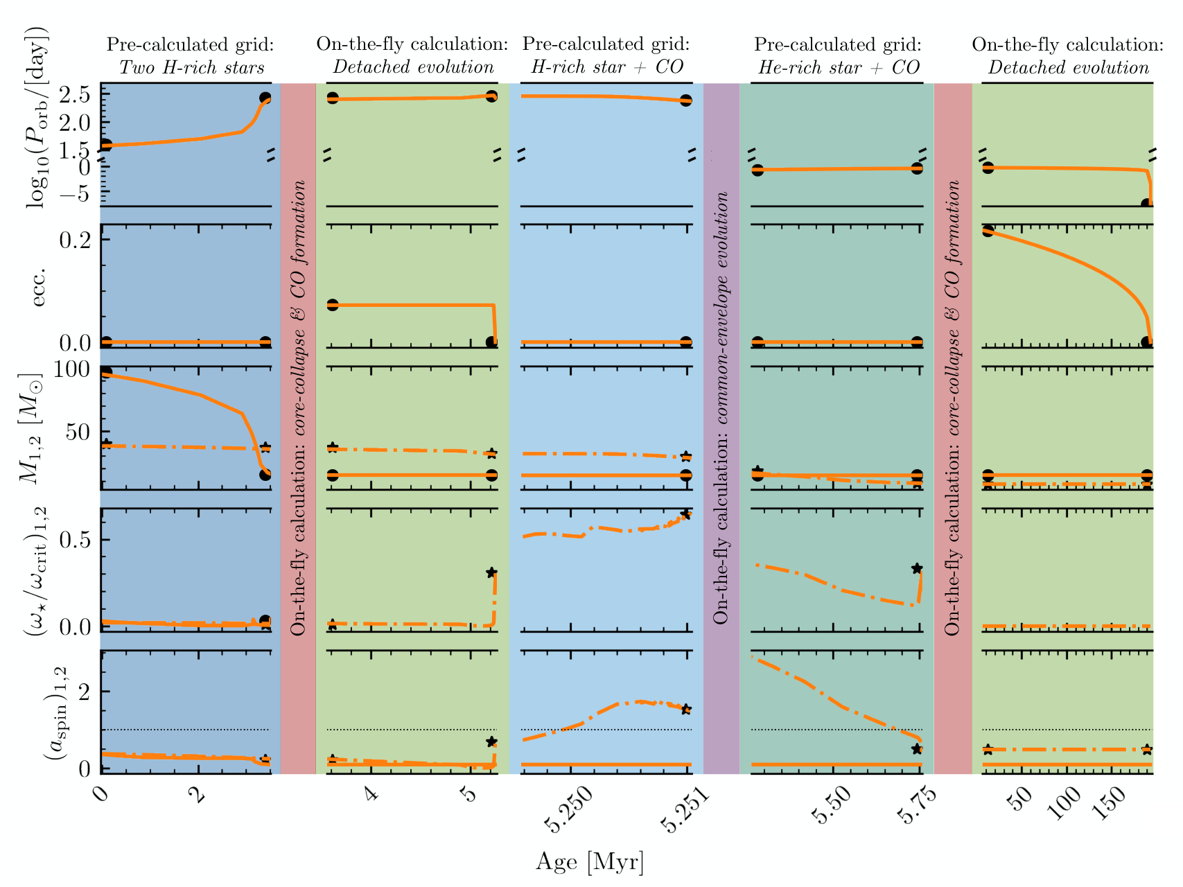
Figure 32 depicts the complete evolution of one particular binary from ZAMS to the formation of a BBH system that merges within a Hubble time. Each vertical, colored band indicates an extended stage of a binary’s evolution, whereas the two core-collapse events and the CE phase are essentially instantaneous processes, occurring in between the other, extended phases.
The initial masses of the system are , in a days circular orbit. The first part of the evolution of the system is based on the HMS–HMS binary grid (Section V.5), and its subsequent evolution is followed either through the nearest neighbor interpolation (orange lines) or through initial–final interpolation (black dots; using our classification and interpolation methods) for the same initial configuration. In both cases we adopt the same SN kick after the two core-collapse episodes in order to compare them as close as possible.
The system does not experiences mass transfer before the first supernova, however the primary experience strong stellar wind mass loss during the Wolf–Rayet phase which widens the orbit . Shortly after the primary collapses into a BH with a low . The subsequent detached evolution (Section VIII.1) of the mildly eccentric system (due to the BH natal kick), after matching the companion of the BH to a single star grid, leads to a small increase of the period predominantly due to winds. Eventually the secondary star fills its Roche lobe at periastron, where we assume that the system circularizes. Mass transfer onto the BH is interpolated through the binary grid of COs with H-star companions (Section V.6) and lasts for a few thousand years, becoming unstable and leading to a CE episode (Section VIII.2). The system survives the process, forming a tight binary comprised of a BH with a stripped He star on a day orbit. Tidal forces become important in this tight orbit, spinning up the He star (Section V.7), which eventually also forms a mildly spinning () BH of . The two BHs merge after 183 Myr from birth, due to gravitational wave radiation.
We have specifically chosen a binary where the differences between the nearest neighbor and initial–final interpolation schemes are relatively small, so that we can accurately display how the binary evolves through each step. Differences between the two evolution options for binaries in general are significantly larger, and the initial–final interpolation scheme is our default choice.
The binary shown in Figure 32 was evolved using our default configuration, although we have purpose-built POSYDON to be modular. Throughout the previous sections we have described possible changes to physical prescriptions that a user can make. However, a user can also easily supplement their own functions for specific steps, or even define the entire binary flow.
Finally, for debugging we keep track of any errors or warnings raised throughout a binary’s evolution. This allows us to isolate the problematic step for a binary, or a stellar and binary state–event combination that our flow structure cannot handle. This error tracking can be especially useful for user-defined steps and flow structures.
X How POSYDON Evolves a Binary Population
Generating a model binary population for comparison to observations requires two separate steps: initializing individual binaries and then evolving those binaries, which we describe in Section X.1 and Section X.2 below. Finally, in Section X.3 we describe a sample binary population evolved with POSYDON.

X.1 Initialization
The primary function of POSYDON is to produce synthetic populations of binaries which requires evolving a random distribution of binaries from ZAMS. We generate an initial population by sampling binary parameters from standard distributions.
Component Masses: For the primary component mass of a binary, we implement initial mass functions (IMF) from Salpeter 1955; Kroupa et al. 1993; Kroupa 2001. By default we use the Kroupa 2001 IMF in the range with . Then the secondary component mass is given by drawing the mass ratio from a flat distribution with .
Orbital Parameters: For a binary population’s initial orbital period, Sana et al. 2013 describe a power-law in log-space, while Opik’s Law describes a log-flat distribution in orbital separation rather than orbital period space (Abt 1983).
In POSYDON we allow for both models to be adopted, with our default being Sana et al. 2013. The minimum orbital period is set by systems that undergo RLO at ZAMS, and a default maximum orbital period to be . The orbital period distribution from Sana et al. 2013 is undefined for day; therefore, we extend this distribution so that it is uniform in space down to a of 0.35 days. We further set the maximum to . Although binaries may form at wider separations, we choose this upper limit to account for all interacting binary models (e.g., Figure 9).
Since we only model circular binaries in our detailed binary-star models with the MESA code, the binary eccentricity at ZAMS is set to zero (see Section IV and Section VIII.1). Since we plan to generalize this assumption in future work, we also add the option to generate from a thermal distribution (Duquennoy & Mayor 1991).
Star-formation History: To account for the star-formation history (SFH) of a binary population, we assign to each binary in the population the same maximum age. Then different star-formation rates (SFRs) can be modeled by modifying the distribution of birth times. In POSYDON we offer two options for the SFR: a burst of star formation or a constant SFR. For the burst model, all binaries have identical birth times some number of years prior to the end of the simulation. For a constant SFR, we randomly generate birth times from a uniform distribution within a user-defined range. The average metallicity of the Galaxy and the greater Universe evolve over time, but this is something that we cannot currently model accurately, as our grids of models presented in v1.0 of POSYDON are only calculated for stars at solar metallicity.
X.2 Evolution
Evolving a population of ZAMS binaries initialized using the distributions described in Section X.1 requires implementing the procedure outlined in Section IX for each binary. In POSYDON we have created an overarching BinaryPopulation class which is a container for a list of individual BinaryStar instances. Each BinaryStar instance is then iteratively evolved until the entire population has been processed.
The BinaryPopulation class contains a number of additional capabilities to efficiently and easily evolve populations of binaries. First, evolved populations are automatically saved in an efficient hdf5 file format with two datasets: one that contains each binary as a single line providing both its initial and final states, and a second dataset that contains the entire evolutionary history of each binary. Second, populations can be evolved either serially or in parallel, so that large ( binaries) populations can be run quickly on a high-performance computing cluster. Third, we have implemented routines that catch and keep warnings and errors from each binary, so that the code does not crash when a single binary fails to complete its evolution due to a bug. We have found this to be useful for identifying and resolving coding bugs when implementing new physical prescriptions. Last, we have implemented various routines that allow a user to easily select only certain types of binaries (e.g., only BBHs or only double COs).
We envision that a typical user will interact primarily with the BinaryPopulation class and its associated SimulationProperties class, which when combined provide the interface for customizing a particular user’s binary population synthesis needs.
X.3 Example Population
To demonstrate the results of a binary population synthesis run with POSYDON, we construct a basic population of binaries generated with the default initial conditions described in Section X.1. We choose a constant star formation history over the past 10 Gyr. The simulation on our high performance computing cluster, Trident, takes approximately 2 hours of wall time using 5 nodes, each with 20 cores, i.e., less than 1 s of CPU time per binary.
From the resulting binaries, we select those that evolve into bound NS–NS, NS–BH, or BH–BH systems. The present-day properties of these binaries are provided in Figure 33; this can be compared with the results of other studies, e.g., Figure 3 from Breivik et al. 2020 with similar initial conditions at solar metallicity. Overall we find good agreement reaffirming that the code is producing reasonable results. In the left two panels, we show distributions of the component compact object masses. Our NS masses are in very close agreement with those of Breivik et al. 2020, although the BHs we produce extend to larger masses. The reason is that current stellar models with stellar structure and evolution parameters calibrated to the latest observations (e.g., overshoorting, etc) produce cores more massive compared to those in the late-nineties models used in rapid BPS codes. The third panel from the left shows the semi-latus rectum of the population. Again, the distribution results are qualitatively similar, with a preference for NS–NS systems at smaller , and NN–BH and BH–BH systems having larger . Finally, the rightmost panel of Figure 33 shows an increasing formation timescale (from ZAMS to the second SN) as we move from BH–BH to NS–BH to NS–NS systems. This is expected since BHs tend to form from more massive systems that complete their evolution more quickly. Our binary CO populations appear morphologically similar to those produced by COSMIC and described in Breivik et al. 2020. We will undertake detailed descriptions of the specific binary populations of interest to separate, science studies.
XI Summary and Future work
Here we present POSYDON, a new, next-generation computational tool for general population synthesis of single and binary stars. POSYDON incorporates full stellar structure and evolution sequences for interacting binaries, using the MESA code. Compared to other existing, binary population synthesis code there are significant advances: (i) binary evolution is treated self-consistently without analytical fits of single-star evolutionary tracks and the need for simplified or artificial recipes to emulate the behavior of stars in interacting binaries; (ii) initial-final classification and interpolation methods trained on the pre-calculated grids of binary evolution models, allowing general synthetic simulations of binary populations. The code base along with the existing evolutionary-track grids are publicly available through the POSYDON collaboration’s web portal (https://posydon.org) along with full documentation and tutorials for how to use the code. An advanced query system is also available for users to be able to mine the grids of single- and binary-star evolutionary tracks and download relevant data using pre-programmed and customized queries (Teng et al. 2021a; Teng et al. 2021b, e.g.,). Finally, we provide a user-friendly web-application that allows a user to perform small-scale simulations with POSYDON online, without the need of code installation and configuration.
Compared to current rapid population synthesis codes POSYDON has a smaller set of free parameters, for many of which there are already multiple options for the user to choose from. The code structure is modular and an advanced user is able to implement their own choices of evolutionary parameters; from as simple as changing the initial properties of the binaries to as complex as incorporating their own custom-made evolutionary-track grids. In this first instrument POSYDON paper we describe in detail the first version of the code, but technical and astrophysical advancements are ongoing and improved code versions will be released in the near and long-term future.
Our focus on the technical front is on classification and interpolation methods. Our current process of first classifying the grids and then performing interpolation can lead to errors propagating throughout the pipeline. Instead these two could be combined into a joint treatment to reduce errors, making additional use of covariances between the different grid types (Singh et al. 2016). We will also explore adopting kernelized-interpolation approaches (Wilson & Nickisch 2015; Gardner et al. 2018; Narayan et al. 2021, i.e.,). To illustrate the use of such an approach, it is observed in Figure 22 that the confusion matrix for our grid of He-rich stars with compact object companions has a lower accuracy for unstable mass transfer. This is perhaps due to the non-linearly separable decision boundary, as visible in Figure 21. Adopting a kernelized-interpolation technique has the potential to increase the class-specific interpolation accuracy. In particular, kernel-based approaches such as support vector machines and Gaussian processes may prove fruitful. In principle, we may also use a neural networks. Also, improvements can be made by adopting non-Euclidean metrics when defining our distance functions in our -nearest neighbors classifiers in Section VII.2.
Apart from methods exploration for the existing classification and interpolation processes, we will focus on the next step of interpolations critical for astrophysical studies: interpolation between whole evolutionary tracks along time. This is a challenging problem that is of particular interest for any study that requires tracking binary properties as a function of their age (e.g., X-ray binary luminosities). In parallel, we are already working on increasing the computational efficiency of building the pre-computed grids necessary for future POSYDON versions. Specifically, for any future grid development, we will take advantage of a new active-learning method developed by our team (Rocha et al. 2022) that allows us to achieve the same classification and interpolation accuracies with a significantly smaller MESA tracks, by dynamically placing them at class boundaries in the parameter space. Such dynamic placement, informed by active learning, leads to grids with non-regular, but smart placement of evolutionary tracks. This work becomes more critical as we expand to more metallicities and add eccentricity as another dimension in order to keep the POSYDON package sizes appropriate for downloads.
The first version of POSYDON is fully functional as an astrophysical tool in the sense that it can be used for complete simulations of binary populations from ZAMS to either formation of a binary with two compact objects or binary distractions (stellar merger or binary disruption), but it is still limited in two ways: our current pre-computed grids are for primaries massive enough to likely form a NS or a BH and are calculated at solar metallicity only. Our next version will expand to a grid of metallicities appropriate for populations across the Universe instead of just the Milky Way. Challenges related to the convergence of single- and binary-star evolutionary models often depend on metallicity, e.g. because the different opacities will results in massive stars reaching the Eddinghton limit within their interiors at different mass ranges and evolutionary phases. Typically, however, such challenges become less severe with decreasing metallicity. Interpolation across metallicities will be a follow-up step as well, once grids at a sufficient number of metallicities have been computed. All the interpolation and classification methods we have developed scale naturally to additional dimensions in the initial conditions parameter space. Further we will expand our grids to low-mass primaries so populations with WDs can also be modeled. Expansion of the grids will inevitably increase data set sizes proportionally. The development of interpolation methods for not only the final properties of each grid but also the entire evolutionary tracks, which is one of our primary future objectives, will allow future POSYDON releases to come only with with the pre-trained interpolation objects. The latter are expected to have a significantly smaller data footprint compared to the downsampled grids we currently ship with POSYDON.
We will also continue to improve the physics treatment of binary evolution. Specifically we are already working on three improvements: (i) in this first version our treatment of the CE phase, once dynamical instability is recognized (taking into account the full stellar structure of the RLO star), is similar to what is done in pBPS codes, apart from the self-consistent calculation of the CE’s binding energy. However, since we model binaries with MESA, we are able to treat the phase in a more physical way, either by following the CE inspiral self-consistently using one-dimensional hydrodynamic simulations (Fragos et al. 2019, e.g.,) or by following the long-term response of the RLO star to losing its envelope on a very high rate and have its Roche lobe shrinking rapidly (Marchant et al. 2021; Gallegos-Garcia et al. 2021, e.g.,). One of the objectives of the next version of POSYDON will be to improve the physics of our CE treatment. (ii) like all binary population modeling to date, we assume that binaries circularize instantly upon RLO and for this reason we also assume that all ZAMS binaries are circular. However, the physics of secular binary evolution through mass transfer in eccentric orbits has been fully developed recently (Sepinsky et al. 2007; Sepinsky et al. 2009; Sepinsky et al. 2010; Dosopoulou & Kalogera 2016a; Dosopoulou & Kalogera 2016b; Hamers et al. 2021) and will be implemented in future POSYDON versions. (iii) Most recently more physical models for magnetic braking have been developed and calibrated against single-star rotational-velocity data (Van & Ivanova 2019; Van & Ivanova 2021; Gossage et al. 2021, e.g.,) and we will use them to update the options for magnetic braking evolution in binaries.
| Name | Description | Unit |
|---|---|---|
| he_core_mass | Helium core mass. | |
| c_core_mass | Carbon core mass. | |
| o_core_mass | Oxygen core mass. | |
| he_core_radius**footnotemark: | Helium core radius. | |
| c_core_radius**footnotemark: | Carbon core radius. | |
| o_core_radius**footnotemark: | Oxygen core radius. | |
| center_h1 | Center mass fraction. | |
| center_he4 | Center mass fraction. | |
| center_c12**footnotemark: | Center mass fraction. | |
| center_n14**footnotemark: | Center mass fraction. | |
| center_o16**footnotemark: | Center mass fraction. | |
| surface_h1**footnotemark: | Surface mass fraction. | |
| surface_he4**footnotemark: | Surface mass fraction. | |
| surface_c12**footnotemark: | Surface mass fraction. | |
| surface_n14**footnotemark: | Surface mass fraction. | |
| surface_o16**footnotemark: | Surface mass fraction. | |
| c12_c12**footnotemark: | Decimal logarithm of the burning power from the reaction | |
| center_gamma**footnotemark: | Plasma coupling parameter, ratio of the Coulomb to thermal energy. | |
| avg_c_in_c_core | Average abundance at carbon core. | |
| surf_avg_omega**footnotemark: | Average surface angular velocity. | |
| surf_avg_omega_div_omega_crit**footnotemark: | Ratio of the average and critical surface angular velocity. | |
| log_LH**footnotemark: | Decimal logarithm of the hydrogen burning power. | |
| log_LHe**footnotemark: | Decimal logarithm of the helium burning power. | |
| log_LZ**footnotemark: | Decimal logarithm of the total burning power excluding LH and LHe and photodisintegration. | |
| log_Lnuc**footnotemark: | Decimal logarithm of the total nuclear burning power. | |
| log_Teff | Decimal logarithm of the effective temperature. | |
| log_L | Decimal logarithm of the luminosity. | |
| log_R | Decimal logarithm of the radius. | |
| total_moment_of_inertia | Total momentum of inertia. | |
| spin_parameter**footnotemark: | Dimensionless stellar spin parameter. | |
| log_total_angular_momentum | Decimal logarithm of the total angular momentum. | |
| conv_env_top_mass**footnotemark: | Mass coordinate of the top boundary of the outermost convective region. | |
| conv_env_bot_mass**footnotemark: | Mass coordinate of the bottom boundary of the outermost convective region. | |
| conv_env_top_radius**footnotemark: | Radial coordinate of the top boundary of the outermost convective region. | |
| conv_env_bot_radius**footnotemark: | Radial coordinate of the bottom boundary of the outermost convective region. | |
| conv_env_turnover_time_g**footnotemark: | Global convective turnover time. | |
| conv_env_turnover_time_l_b**footnotemark: | Local convective turnover time half of a scale height above the outermost convective zone bottom boundary. | |
| conv_env_turnover_time_l_t**footnotemark: | Local turnover time one scale height above the outermost convective zone bottom boundary. | |
| envelope_binding_energy**footnotemark: | Binding energy of the envelope. | |
| mass_conv_reg_fortides**footnotemark: | Mass of the most important convective region for equilibrium tides, as defined in Eq. (7). | |
| thickness_conv_reg_fortides**footnotemark: | Thickness of the most important convective region for equilibrium tides, as defined in Eq. (7). | |
| radius_conv_reg_fortides**footnotemark: | Radial coordinate of the most important convective region for equilibrium tides, as defined in Eq. (7). | |
| lambda_CE_1cent**footnotemark: | Common-envelope parameter of the envelope binding energy for core-envelope boundary where hydrogen mass fraction becomes lower than 1%. | |
| lambda_CE_10cent**footnotemark: | Common-envelope parameter of the envelope binding energy for core-envelope boundary where hydrogen mass fraction becomes lower than 10%. | |
| lambda_CE_30cent**footnotemark: | Common-envelope parameter of the envelope binding energy for core-envelope boundary where hydrogen mass fraction becomes lower than 30%. | |
| co_core_mass | Carbon–oxygen core mass. | |
| co_core_radius**footnotemark: | Carbon–oxygen core radius. | |
| lambda_CE_pure_He_star_10cent**footnotemark: | Common-envelope parameter of the He-rich envelope binding energy for core-envelope boundary where the sum of hydrogen and helium mass fraction becomes lower than 10%. | |
| log_L_div_Ledd**footnotemark: | Decimal logarithm of the ratio of the luminosity and Eddington luminosity. |
| Name | Description | Unit |
|---|---|---|
| model_number**footnotemark: | The model number of the final state | |
| age**footnotemark: | Binary age | |
| star_1_mass | Mass of the first star | |
| star_2_mass | Mass of the second star | |
| period_days | Orbital period in days | |
| binary_separation | Binary separation | |
| lg_system_mdot_1 | Decimal logarithm of rate of mass loss from the system from around the first star due to inefficient mass transfer | |
| lg_system_mdot_2 | Decimal logarithm of rate of mass loss from the system from around the second star due to inefficient mass transfer | |
| lg_wind_mdot_1**footnotemark: | Decimal logarithm of rate of mass loss of the first star due to wind | |
| lg_wind_mdot_2**footnotemark: | Decimal logarithm of rate of mass loss of the second star due to wind | |
| lg_mstar_dot_1**footnotemark: | Decimal logarithm of rate of mass loss of the first star | |
| lg_mstar_dot_2**footnotemark: | Decimal logarithm of rate of mass loss of the second star | |
| lg_mtransfer_rate | Decimal logarithm of mass-transfer rate | |
| xfer_fraction**footnotemark: | Mass-transfer fraction | |
| rl_relative_overflow_1**footnotemark: | Roche lobe overflow of the first star in units of donor Roche lobe radii | |
| rl_relative_overflow_2**footnotemark: | Roche lobe overflow of the second star in units of donor Roche lobe radii | |
| trap_radius**footnotemark: | Trapping radius | |
| acc_radius**footnotemark: | Radius of the compact object | |
| t_sync_rad_1**footnotemark: | Tidal synchronization time-scale of the first star for stars with radiative envelopes | |
| t_sync_conv_1**footnotemark: | Tidal synchronization time-scale of the first star for stars with convective envelopes | |
| t_sync_rad_2**footnotemark: | Tidal synchronization time-scale of the second star for stars with radiative envelopes | |
| t_sync_conv_2**footnotemark: | Tidal synchronization time-scale of the second star for stars with convective envelopes |
| Name | Description | Unit |
|---|---|---|
| radius | Radius at the outer boundary of the zone. | |
| mass**footnotemark: | Mass coordinate of the outer boundary of the zone. | |
| logRho | Decimal logarithm of the density at the center of the zone. | |
| omega | Angular velocity. | |
| energy**footnotemark: | Specific internal energy. | |
| x_mass_fraction_H**footnotemark: | Mass fraction of all isotopes with atomic number 1. | |
| y_mass_fraction_He**footnotemark: | Mass fraction of all isotopes with atomic number 2. | |
| z_mass_fraction_metals**footnotemark: | Mass fraction of all elements except for those in x_mass_fraction_H and y_mass_fraction_He | |
| neutral_fraction_H**footnotemark: | Fraction of neutral hydrogen (HI) of all the . | |
| neutral_fraction_He**footnotemark: | Fraction of neutral helium (HeI) of all the . | |
| avg_charge_He**footnotemark: | Average charge of all the isotopes. | electron charge [] |
| Name | Description | Unit |
|---|---|---|
| termination_flag_1 | Termination reason from MESA output, or reach cluster timelimit. | |
| termination_flag_2 | RLO state (indicating which star is the donor), or contact_during_MS in case of stellar merger. | |
| termination_flag_3 | State of primary star. | |
| termination_flag_4 | State of secondary star. | |
| interpolation_class | Classification based on termination flags 1 and 2, indicating broad groups based on mass transfer. | |
| surface_other | Surface abundance fraction of elements excluding , , , , . | |
| center_other | Central abundance fraction of elements excluding , , , , . | |
| direct_state | CO state for the direct collapse prescription of the star. | |
| direct_SN_type | SN type for the direct collapse prescription of the star. | |
| direct_f_fb | Fallback mass fraction for the direct collapse prescription of the star. | |
| direct_mass | CO mass for the direct collapse prescription of the star. | |
| direct_spin | CO spin for the direct collapse prescription of the star. | |
| Fryer+12-rapid_state | CO state for the Fryer et al. 2012 rapid prescription of the star. | |
| Fryer+12-rapid_SN_type | SN type for the Fryer et al. 2012 rapid prescription of the star. | |
| Fryer+12-rapid_f_fb | Fallback mass fraction for the Fryer et al. 2012 rapid prescription of the star. | |
| Fryer+12-rapid_mass | CO mass for the Fryer et al. 2012 rapid prescription of the star. | |
| Fryer+12-rapid_spin | CO spin for the Fryer et al. 2012 rapid prescription of the star. | |
| Fryer+12-delayed_state | CO state for the Fryer et al. 2012 delayed prescription of the star. | |
| Fryer+12-delayed_SN_type | SN type for the Fryer et al. 2012 delayed prescription of the star. | |
| Fryer+12-delayed_f_fb | Fallback mass fraction for the Fryer et al. 2012 delayed prescription of the star. | |
| Fryer+12-delayed_mass | CO mass for the Fryer et al. 2012 delayed prescription of the star. | |
| Fryer+12-delayed_spin | CO spin for the Fryer et al. 2012 delayed prescription of the star. | |
| Sukhbold+16-engineN20_state | CO state for the Sukhbold et al. 2016 N20 engine prescription of the star. | |
| Sukhbold+16-engineN20_SN_type | SN type for the Sukhbold et al. 2016 N20 engine prescription of the star. | |
| Sukhbold+16-engineN20_f_fb | Fallback mass fraction for the Sukhbold et al. 2016 N20 engine prescription of the star. | |
| Sukhbold+16-engineN20_mass | CO mass for the Sukhbold et al. 2016 N20 engine prescription of the star. | |
| Sukhbold+16-engineN20_spin | CO spin for the Sukhbold et al. 2016 N20 engine prescription of the star. | |
| Patton&Sukhbold20-engineN20_state | CO state for the Patton & Sukhbold 2020 N20 engine prescription of the star. | |
| Patton&Sukhbold20-engineN20_SN_type | SN type for the Patton & Sukhbold 2020 N20 engine prescription of the star. | |
| Patton&Sukhbold20-engineN20_f_fb | Fallback mass fraction for the Patton & Sukhbold 2020 N20 engine prescription of the star. | |
| Patton&Sukhbold20-engineN20_mass | CO mass for the Patton & Sukhbold 2020 N20 engine prescription of the star. | |
| Patton&Sukhbold20-engineN20_spin | CO spin for the Patton & Sukhbold 2020 N20 engine prescription of the star. | |
| avg_c_in_c_core_at_He_depletion | Average carbon 12 abundance at carbon core at the state of He depletion of the star. | |
| co_core_mass_at_He_depletion | Carbon–oxygen core mass at the state of He depletion of the star. | |
| m_core_CE_1cent | Mass of the hydrogen-deficient (i.e. helium) core, with the core-envelope boundary defined as the outermost layer where the hydrogen mass fraction drops below 1%. | |
| m_core_CE_10cent | As m_core_CE_1cent, but for hydrogen mass fraction of 10%. | |
| m_core_CE_10cent | As m_core_CE_1cent, but for hydrogen mass fraction of 30%. | |
| m_core_CE_pure_He_star_10cent | Mass of the hydrogen- and helium-deficient (i.e., carbon–oxygen) core, with the core–envelope boundary defined as the outermost layer where the sum of hydrogen and helium mass fraction drops below 10%. | |
| r_core_CE_1cent | Radial coordinate of the core as defined in m_core_CE_1cent. | |
| r_core_CE_10cent | Radial coordinate of the core as defined in m_core_CE_10cent. | |
| r_core_CE_30cent | Radial coordinate of the core as defined in m_core_CE_30cent. | |
| r_core_CE_pure_He_star_10cent | Radial coordinate of the core as defined in m_core_CE_pure_He_star_10cent. |
References
- Aasi et al. (2015) Aasi, J., Abbott, B. P., Abbott, R., et al. 2015, Classical and Quantum Gravity, 32, 074001, doi: 10.1088/0264-9381/32/7/074001
- Abbott et al. (2016) Abbott, B. P., Abbott, R., Abbott, T. D., et al. 2016, Phys. Rev. Lett., 116, 061102, doi: 10.1103/PhysRevLett.116.061102
- Abbott et al. (2020a) —. 2020a, ApJ, 892, L3, doi: 10.3847/2041-8213/ab75f5
- Abbott et al. (2020b) Abbott, R., Abbott, T. D., Abraham, S., et al. 2020b, ApJ, 896, L44, doi: 10.3847/2041-8213/ab960f
- Abbott et al. (2021) Abbott, R., Abbott, T. D., Acernese, F., et al. 2021, arXiv e-prints, arXiv:2111.03606. https://arxiv.org/abs/2111.03606
- Abt (1983) Abt, H. A. 1983, ARA&A, 21, 343, doi: 10.1146/annurev.aa.21.090183.002015
- Acernese et al. (2015) Acernese, F., Agathos, M., Agatsuma, K., et al. 2015, Classical and Quantum Gravity, 32, 024001, doi: 10.1088/0264-9381/32/2/024001
- Agrawal et al. (2020) Agrawal, P., Hurley, J., Stevenson, S., Szécsi, D., & Flynn, C. 2020, MNRAS, 497, 4549, doi: 10.1093/mnras/staa2264
- Agrawal et al. (2022) Agrawal, P., Szécsi, D., Stevenson, S., Eldridge, J. J., & Hurley, J. 2022, MNRAS, 512, 5717, doi: 10.1093/mnras/stac930
- Ai et al. (2020) Ai, S., Gao, H., & Zhang, B. 2020, ApJ, 893, 146, doi: 10.3847/1538-4357/ab80bd
- Akutsu et al. (2019) Akutsu, T., Ando, M., Arai, K., et al. 2019, Nature Astronomy, 3, 35, doi: 10.1038/s41550-018-0658-y
- Andrews et al. (2015) Andrews, J. J., Farr, W. M., Kalogera, V., & Willems, B. 2015, ApJ, 801, 32, doi: 10.1088/0004-637X/801/1/32
- Artale et al. (2019) Artale, M. C., Giacobbo, N., Mapelli, M., & Esposito, P. 2019, IAU Symposium, 346, 332, doi: 10.1017/S1743921318007627
- Asplund et al. (2009) Asplund, M., Grevesse, N., Sauval, A. J., & Scott, P. 2009, ARA&A, 47, 481, doi: 10.1146/annurev.astro.46.060407.145222
- Böhm-Vitense (1958) Böhm-Vitense, E. 1958, Zeitschrift für Astrophysik, 46, 108
- Bardeen (1970) Bardeen, J. M. 1970, Nature, 226, 64, doi: 10.1038/226064a0
- Barkat et al. (1967) Barkat, Z., Rakavy, G., & Sack, N. 1967, Phys. Rev. Lett., 18, 379, doi: 10.1103/PhysRevLett.18.379
- Batta & Ramirez-Ruiz (2019) Batta, A., & Ramirez-Ruiz, E. 2019, arXiv e-prints, arXiv:1904.04835. https://arxiv.org/abs/1904.04835
- Bavera et al. (2020) Bavera, S. S., Fragos, T., Qin, Y., et al. 2020, A&A, 635, A97, doi: 10.1051/0004-6361/201936204
- Bavera et al. (2021) Bavera, S. S., Fragos, T., Zevin, M., et al. 2021, A&A, 647, A153, doi: 10.1051/0004-6361/202039804
- Begelman (1979) Begelman, M. C. 1979, MNRAS, 187, 237, doi: 10.1093/mnras/187.2.237
- Belczynski et al. (2010) Belczynski, K., Bulik, T., Fryer, C. L., et al. 2010, ApJ, 714, 1217, doi: 10.1088/0004-637X/714/2/1217
- Belczynski et al. (2016) Belczynski, K., Holz, D. E., Bulik, T., & O’Shaughnessy, R. 2016, Nature, 534, 512, doi: 10.1038/nature18322
- Belczynski et al. (2002) Belczynski, K., Kalogera, V., & Bulik, T. 2002, ApJ, 572, 407, doi: 10.1086/340304
- Belczynski et al. (2008) Belczynski, K., Kalogera, V., Rasio, F. A., et al. 2008, ApJS, 174, 223, doi: 10.1086/521026
- Belczynski et al. (2004) Belczynski, K., Kalogera, V., Zezas, A., & Fabbiano, G. 2004, ApJ, 601, L147, doi: 10.1086/382131
- Bhattacharya & van den Heuvel (1991) Bhattacharya, D., & van den Heuvel, E. P. J. 1991, Phys. Rep., 203, 1, doi: 10.1016/0370-1573(91)90064-S
- Bisnovatyi-Kogan (1993) Bisnovatyi-Kogan, G. S. 1993, Astronomical and Astrophysical Transactions, 3, 287, doi: 10.1080/10556799308230566
- Biswas (2021) Biswas, B. 2021, ApJ, 921, 63, doi: 10.3847/1538-4357/ac1c72
- Blaauw (1961) Blaauw, A. 1961, Bull. Astron. Inst. Netherlands, 15, 265
- Bloecker (1995) Bloecker, T. 1995, A&A, 297, 727
- Boersma (1961) Boersma, J. 1961, Bull. Astron. Inst. Netherlands, 15, 291
- Breivik et al. (2018) Breivik, K., Kremer, K., Bueno, M., et al. 2018, ApJ, 854, L1, doi: 10.3847/2041-8213/aaaa23
- Breivik et al. (2020) Breivik, K., Coughlin, S., Zevin, M., et al. 2020, ApJ, 898, 71, doi: 10.3847/1538-4357/ab9d85
- Broekgaarden et al. (2021) Broekgaarden, F. S., Berger, E., Neijssel, C. J., et al. 2021, MNRAS, 508, 5028, doi: 10.1093/mnras/stab2716
- Brott et al. (2011) Brott, I., de Mink, S. E., Cantiello, M., et al. 2011, A&A, 530, A115, doi: 10.1051/0004-6361/201016113
- Burrows & Hayes (1996) Burrows, A., & Hayes, J. 1996, Phys. Rev. Lett., 76, 352, doi: 10.1103/PhysRevLett.76.352
- Burrows & Vartanyan (2021) Burrows, A., & Vartanyan, D. 2021, Nature, 589, 29, doi: 10.1038/s41586-020-03059-w
- Calzetti et al. (2015) Calzetti, D., Lee, J. C., Sabbi, E., et al. 2015, AJ, 149, 51, doi: 10.1088/0004-6256/149/2/51
- Cantiello et al. (2014) Cantiello, M., Mankovich, C., Bildsten, L., Christensen-Dalsgaard, J., & Paxton, B. 2014, ApJ, 788, 93, doi: 10.1088/0004-637X/788/1/93
- Cassisi et al. (2007) Cassisi, S., Potekhin, A. Y., Pietrinferni, A., Catelan, M., & Salaris, M. 2007, ApJ, 661, 1094, doi: 10.1086/516819
- Charbonnel & Zahn (2007) Charbonnel, C., & Zahn, J. P. 2007, A&A, 467, L15, doi: 10.1051/0004-6361:20077274
- Chattopadhyay et al. (2020) Chattopadhyay, D., Stevenson, S., Hurley, J. R., Rossi, L. J., & Flynn, C. 2020, MNRAS, 494, 1587, doi: 10.1093/mnras/staa756
- Choi et al. (2016) Choi, J., Dotter, A., Conroy, C., et al. 2016, ApJ, 823, 102, doi: 10.3847/0004-637X/823/2/102
- Chruslinska et al. (2017) Chruslinska, M., Belczynski, K., Bulik, T., & Gladysz, W. 2017, Acta Astron., 67, 37, doi: 10.32023/0001-5237/67.1.2
- Claeys et al. (2014) Claeys, J. S. W., Pols, O. R., Izzard, R. G., Vink, J., & Verbunt, F. W. M. 2014, A&A, 563, A83, doi: 10.1051/0004-6361/201322714
- Claret & Torres (2017) Claret, A., & Torres, G. 2017, ApJ, 849, 18, doi: 10.3847/1538-4357/aa8770
- Conroy (2013) Conroy, C. 2013, ARA&A, 51, 393, doi: 10.1146/annurev-astro-082812-141017
- Cyburt et al. (2010) Cyburt, R. H., Amthor, A. M., Ferguson, R., et al. 2010, ApJS, 189, 240, doi: 10.1088/0067-0049/189/1/240
- Dalcanton et al. (2012) Dalcanton, J. J., Williams, B. F., Lang, D., et al. 2012, ApJS, 200, 18, doi: 10.1088/0067-0049/200/2/18
- De Donder & Vanbeveren (2003) De Donder, E., & Vanbeveren, D. 2003, New A, 8, 817, doi: 10.1016/S1384-1076(03)00069-1
- de Jager et al. (1988) de Jager, C., Nieuwenhuijzen, H., & van der Hucht, K. A. 1988, A&AS, 72, 259
- de Kool (1990) de Kool, M. 1990, ApJ, 358, 189, doi: 10.1086/168974
- De Marco & Izzard (2017) De Marco, O., & Izzard, R. G. 2017, PASA, 34, e001, doi: 10.1017/pasa.2016.52
- de Mink et al. (2013) de Mink, S. E., Langer, N., Izzard, R. G., Sana, H., & de Koter, A. 2013, ApJ, 764, 166, doi: 10.1088/0004-637X/764/2/166
- de Mink et al. (2007) de Mink, S. E., Pols, O. R., & Hilditch, R. W. 2007, A&A, 467, 1181, doi: 10.1051/0004-6361:20067007
- Delgado & Thomas (1981) Delgado, A. J., & Thomas, H. C. 1981, A&A, 96, 142
- Dewi & Tauris (2000) Dewi, J. D. M., & Tauris, T. M. 2000, A&A, 360, 1043. https://arxiv.org/abs/astro-ph/0007034
- Dominik et al. (2012) Dominik, M., Belczynski, K., Fryer, C., et al. 2012, ApJ, 759, 52, doi: 10.1088/0004-637X/759/1/52
- Dominik et al. (2013) —. 2013, ApJ, 779, 72, doi: 10.1088/0004-637X/779/1/72
- Dominik et al. (2015) Dominik, M., Berti, E., O’Shaughnessy, R., et al. 2015, ApJ, 806, 263, doi: 10.1088/0004-637X/806/2/263
- Dosopoulou & Kalogera (2016a) Dosopoulou, F., & Kalogera, V. 2016a, ApJ, 825, 70, doi: 10.3847/0004-637X/825/1/70
- Dosopoulou & Kalogera (2016b) —. 2016b, ApJ, 825, 71, doi: 10.3847/0004-637X/825/1/71
- Dotter (2016) Dotter, A. 2016, ApJS, 222, 8, doi: 10.3847/0067-0049/222/1/8
- Duquennoy & Mayor (1991) Duquennoy, A., & Mayor, M. 1991, A&A, 500, 337
- Eddington (1926) Eddington, A. S. 1926, The Internal Constitution of the Stars
- Eggenberger et al. (2005) Eggenberger, P., Maeder, A., & Meynet, G. 2005, A&A, 440, L9, doi: 10.1051/0004-6361:200500156
- Eggenberger et al. (2012) Eggenberger, P., Montalbán, J., & Miglio, A. 2012, A&A, 544, L4, doi: 10.1051/0004-6361/201219729
- Eggleton (1971) Eggleton, P. P. 1971, MNRAS, 151, 351, doi: 10.1093/mnras/151.3.351
- Eggleton & Kiseleva-Eggleton (2002) Eggleton, P. P., & Kiseleva-Eggleton, L. 2002, ApJ, 575, 461, doi: 10.1086/341215
- Ekström et al. (2012) Ekström, S., Georgy, C., Eggenberger, P., et al. 2012, A&A, 537, A146, doi: 10.1051/0004-6361/201117751
- Eldridge & Stanway (2022) Eldridge, J. J., & Stanway, E. R. 2022, arXiv e-prints, arXiv:2202.01413. https://arxiv.org/abs/2202.01413
- Eldridge et al. (2017) Eldridge, J. J., Stanway, E. R., Xiao, L., et al. 2017, PASA, 34, e058, doi: 10.1017/pasa.2017.51
- Eldridge & Tout (2004) Eldridge, J. J., & Tout, C. A. 2004, MNRAS, 353, 87, doi: 10.1111/j.1365-2966.2004.08041.x
- Ertl et al. (2016) Ertl, T., Janka, H. T., Woosley, S. E., Sukhbold, T., & Ugliano, M. 2016, ApJ, 818, 124, doi: 10.3847/0004-637X/818/2/124
- Ertl et al. (2020) Ertl, T., Woosley, S. E., Sukhbold, T., & Janka, H. T. 2020, ApJ, 890, 51, doi: 10.3847/1538-4357/ab6458
- Evans et al. (2019) Evans, I. N., Allen, C., Anderson, C. S., et al. 2019, in AAS/High Energy Astrophysics Division, Vol. 17, AAS/High Energy Astrophysics Division, 114.01
- Farmer et al. (2020) Farmer, R., Renzo, M., de Mink, S. E., Fishbach, M., & Justham, S. 2020, ApJ, 902, L36, doi: 10.3847/2041-8213/abbadd
- Farmer et al. (2019) Farmer, R., Renzo, M., de Mink, S. E., Marchant, P., & Justham, S. 2019, ApJ, 887, 53, doi: 10.3847/1538-4357/ab518b
- Ferguson et al. (2005) Ferguson, J. W., Alexander, D. R., Allard, F., et al. 2005, ApJ, 623, 585, doi: 10.1086/428642
- Flannery & van den Heuvel (1975) Flannery, B. P., & van den Heuvel, E. P. J. 1975, A&A, 39, 61
- Fowler & Hoyle (1964) Fowler, W. A., & Hoyle, F. 1964, ApJS, 9, 201, doi: 10.1086/190103
- Fragos et al. (2019) Fragos, T., Andrews, J. J., Ramirez-Ruiz, E., et al. 2019, ApJ, 883, L45, doi: 10.3847/2041-8213/ab40d1
- Fragos et al. (2013a) Fragos, T., Lehmer, B. D., Naoz, S., Zezas, A., & Basu-Zych, A. 2013a, ApJ, 776, L31, doi: 10.1088/2041-8205/776/2/L31
- Fragos & McClintock (2015) Fragos, T., & McClintock, J. E. 2015, ApJ, 800, 17, doi: 10.1088/0004-637X/800/1/17
- Fragos et al. (2008) Fragos, T., Kalogera, V., Belczynski, K., et al. 2008, ApJ, 683, 346, doi: 10.1086/588456
- Fragos et al. (2013b) Fragos, T., Lehmer, B., Tremmel, M., et al. 2013b, ApJ, 764, 41, doi: 10.1088/0004-637X/764/1/41
- Frank et al. (2002) Frank, J., King, A., & Raine, D. J. 2002, Accretion Power in Astrophysics: Third Edition
- Fryer et al. (2012) Fryer, C. L., Belczynski, K., Wiktorowicz, G., et al. 2012, ApJ, 749, 91, doi: 10.1088/0004-637X/749/1/91
- Fuller & Ma (2019) Fuller, J., & Ma, L. 2019, ApJ, 881, L1, doi: 10.3847/2041-8213/ab339b
- Fuller et al. (2019) Fuller, J., Piro, A. L., & Jermyn, A. S. 2019, MNRAS, 485, 3661, doi: 10.1093/mnras/stz514
- Gaia Collaboration et al. (2018) Gaia Collaboration, Brown, A. G. A., Vallenari, A., et al. 2018, A&A, 616, A1, doi: 10.1051/0004-6361/201833051
- Gallegos-Garcia et al. (2021) Gallegos-Garcia, M., Berry, C. P. L., Marchant, P., & Kalogera, V. 2021, ApJ, 922, 110, doi: 10.3847/1538-4357/ac2610
- Gardner et al. (2018) Gardner, J. R., Pleiss, G., Wu, R., Weinberger, K. Q., & Wilson, A. G. 2018, Proceedings of the Twenty-First International Conference on Artificial Intelligence and Statistics, Proceedings of Machine Learning Research. https://arxiv.org/abs/1802.08903
- Giacobbo & Mapelli (2019) Giacobbo, N., & Mapelli, M. 2019, MNRAS, 482, 2234, doi: 10.1093/mnras/sty2848
- Giacobbo et al. (2018) Giacobbo, N., Mapelli, M., & Spera, M. 2018, MNRAS, 474, 2959, doi: 10.1093/mnras/stx2933
- Gossage et al. (2021) Gossage, S., Dotter, A., Garraffo, C., et al. 2021, ApJ, 912, 65, doi: 10.3847/1538-4357/abebdf
- Graham et al. (2019) Graham, M. J., Kulkarni, S. R., Bellm, E. C., et al. 2019, PASP, 131, 078001, doi: 10.1088/1538-3873/ab006c
- Habets (1986) Habets, G. M. H. J. 1986, A&A, 167, 61
- Hamers & Dosopoulou (2019) Hamers, A. S., & Dosopoulou, F. 2019, ApJ, 872, 119, doi: 10.3847/1538-4357/ab001d
- Hamers et al. (2021) Hamers, A. S., Rantala, A., Neunteufel, P., Preece, H., & Vynatheya, P. 2021, Monthly Notices of the Royal Astronomical Society, 502, 4479–4512, doi: 10.1093/mnras/stab287
- Harris et al. (2020) Harris, C. R., Millman, K. J., van der Walt, S. J., et al. 2020, Nature, 585, 357–362, doi: 10.1038/s41586-020-2649-2
- Heger & Langer (1998) Heger, A., & Langer, N. 1998, A&A, 334, 210
- Heger & Langer (2000) —. 2000, ApJ, 544, 1016, doi: 10.1086/317239
- Heger et al. (2000) Heger, A., Langer, N., & Woosley, S. E. 2000, ApJ, 528, 368, doi: 10.1086/308158
- Heger et al. (2005) Heger, A., Woosley, S. E., & Spruit, H. C. 2005, ApJ, 626, 350, doi: 10.1086/429868
- Herwig (2000) Herwig, F. 2000, A&A, 360, 952. https://arxiv.org/abs/astro-ph/0007139
- Hjellming & Webbink (1987) Hjellming, M. S., & Webbink, R. F. 1987, ApJ, 318, 794, doi: 10.1086/165412
- Hobbs et al. (2005) Hobbs, G., Lorimer, D. R., Lyne, A. G., & Kramer, M. 2005, MNRAS, 360, 974, doi: 10.1111/j.1365-2966.2005.09087.x
- Hopkins et al. (2011) Hopkins, P. F., Quataert, E., & Murray, N. 2011, MNRAS, 417, 950, doi: 10.1111/j.1365-2966.2011.19306.x
- Hopkins et al. (2012) —. 2012, MNRAS, 421, 3522, doi: 10.1111/j.1365-2966.2012.20593.x
- Hunter (2007) Hunter, J. D. 2007, Computing in Science and Engineering, 9, 90, doi: 10.1109/MCSE.2007.55
- Hurley et al. (2000) Hurley, J. R., Pols, O. R., & Tout, C. A. 2000, MNRAS, 315, 543, doi: 10.1046/j.1365-8711.2000.03426.x
- Hurley et al. (2002) Hurley, J. R., Tout, C. A., & Pols, O. R. 2002, MNRAS, 329, 897, doi: 10.1046/j.1365-8711.2002.05038.x
- Hut (1981) Hut, P. 1981, A&A, 99, 126
- Iben (1991) Iben, Icko, J. 1991, ApJS, 76, 55, doi: 10.1086/191565
- Iglesias & Rogers (1996) Iglesias, C. A., & Rogers, F. J. 1996, ApJ, 464, 943, doi: 10.1086/177381
- Ivanova et al. (2020) Ivanova, N., Justham, S., & Ricker, P. 2020, Common Envelope Evolution, doi: 10.1088/2514-3433/abb6f0
- Ivanova et al. (2013) Ivanova, N., Justham, S., Chen, X., et al. 2013, A&A Rev., 21, 59, doi: 10.1007/s00159-013-0059-2
- Ivezić et al. (2014) Ivezić, Ž., Connolly, A., Vanderplas, J., & Gray, A. 2014, Statistics, Data Mining and Machine Learning in Astronomy (Princeton University Press)
- Izzard et al. (2006) Izzard, R. G., Dray, L. M., Karakas, A. I., Lugaro, M., & Tout, C. A. 2006, A&A, 460, 565, doi: 10.1051/0004-6361:20066129
- Izzard et al. (2009) Izzard, R. G., Glebbeek, E., Stancliffe, R. J., & Pols, O. R. 2009, A&A, 508, 1359, doi: 10.1051/0004-6361/200912827
- Izzard et al. (2004) Izzard, R. G., Tout, C. A., Karakas, A. I., & Pols, O. R. 2004, MNRAS, 350, 407, doi: 10.1111/j.1365-2966.2004.07446.x
- Janka (2012) Janka, H.-T. 2012, Annual Review of Nuclear and Particle Science, 62, 407, doi: 10.1146/annurev-nucl-102711-094901
- Janka (2013) —. 2013, MNRAS, 434, 1355, doi: 10.1093/mnras/stt1106
- Janka et al. (2007) Janka, H. T., Langanke, K., Marek, A., Martínez-Pinedo, G., & Müller, B. 2007, Phys. Rep., 442, 38, doi: 10.1016/j.physrep.2007.02.002
- Janka & Mueller (1994) Janka, H. T., & Mueller, E. 1994, A&A, 290, 496
- Jones et al. (2014) Jones, S., Hirschi, R., & Nomoto, K. 2014, ApJ, 797, 83, doi: 10.1088/0004-637X/797/2/83
- Junker & Schaefer (1992) Junker, W., & Schaefer, G. 1992, MNRAS, 254, 146, doi: 10.1093/mnras/254.1.146
- Kaiser et al. (2002) Kaiser, N., Aussel, H., Burke, B. E., et al. 2002, in Society of Photo-Optical Instrumentation Engineers (SPIE) Conference Series, Vol. 4836, Survey and Other Telescope Technologies and Discoveries, ed. J. A. Tyson & S. Wolff, 154–164, doi: 10.1117/12.457365
- Kalogera (1996) Kalogera, V. 1996, ApJ, 471, 352, doi: 10.1086/177974
- Kalogera & Lorimer (2000) Kalogera, V., & Lorimer, D. R. 2000, ApJ, 530, 890, doi: 10.1086/308417
- Kim et al. (2021) Kim, M., Kim, Y.-M., Sung, K. H., Lee, C.-H., & Kwak, K. 2021, A&A, 650, A139, doi: 10.1051/0004-6361/202038126
- King & Begelman (1999) King, A. R., & Begelman, M. C. 1999, ApJ, 519, L169, doi: 10.1086/312126
- King & Kolb (1999) King, A. R., & Kolb, U. 1999, MNRAS, 305, 654, doi: 10.1046/j.1365-8711.1999.02482.x
- Kinugawa et al. (2020) Kinugawa, T., Nakamura, T., & Nakano, H. 2020, MNRAS, 498, 3946, doi: 10.1093/mnras/staa2511
- Kippenhahn et al. (1980) Kippenhahn, R., Ruschenplatt, G., & Thomas, H. C. 1980, A&A, 91, 175
- Klencki et al. (2018) Klencki, J., Moe, M., Gladysz, W., et al. 2018, A&A, 619, A77, doi: 10.1051/0004-6361/201833025
- Klencki et al. (2021) Klencki, J., Nelemans, G., Istrate, A. G., & Chruslinska, M. 2021, A&A, 645, A54, doi: 10.1051/0004-6361/202038707
- Kolb & Ritter (1990) Kolb, U., & Ritter, H. 1990, A&A, 236, 385
- Korol et al. (2020) Korol, V., Toonen, S., Klein, A., et al. 2020, A&A, 638, A153, doi: 10.1051/0004-6361/202037764
- Kroupa (2001) Kroupa, P. 2001, MNRAS, 322, 231, doi: 10.1046/j.1365-8711.2001.04022.x
- Kroupa et al. (1993) Kroupa, P., Tout, C. A., & Gilmore, G. 1993, MNRAS, 262, 545, doi: 10.1093/mnras/262.3.545
- Kruckow et al. (2018) Kruckow, M. U., Tauris, T. M., Langer, N., Kramer, M., & Izzard, R. G. 2018, MNRAS, 481, 1908, doi: 10.1093/mnras/sty2190
- Kruckow et al. (2016) Kruckow, M. U., Tauris, T. M., Langer, N., et al. 2016, A&A, 596, A58, doi: 10.1051/0004-6361/201629420
- Kudritzki & Puls (2000) Kudritzki, R.-P., & Puls, J. 2000, ARA&A, 38, 613, doi: 10.1146/annurev.astro.38.1.613
- Landry et al. (2020) Landry, P., Essick, R., & Chatziioannou, K. 2020, Phys. Rev. D, 101, 123007, doi: 10.1103/PhysRevD.101.123007
- Langer (1998) Langer, N. 1998, A&A, 329, 551
- Langer et al. (1983) Langer, N., Fricke, K. J., & Sugimoto, D. 1983, A&A, 126, 207
- Langer et al. (2020) Langer, N., Schürmann, C., Stoll, K., et al. 2020, A&A, 638, A39, doi: 10.1051/0004-6361/201937375
- Laplace et al. (2020) Laplace, E., Götberg, Y., de Mink, S. E., Justham, S., & Farmer, R. 2020, A&A, 637, A6, doi: 10.1051/0004-6361/201937300
- Laplace et al. (2021) Laplace, E., Justham, S., Renzo, M., et al. 2021, A&A, 656, A58, doi: 10.1051/0004-6361/202140506
- Lattimer & Prakash (2010) Lattimer, J. M., & Prakash, M. 2010, arXiv e-prints, arXiv:1012.3208. https://arxiv.org/abs/1012.3208
- Lattimer & Yahil (1989) Lattimer, J. M., & Yahil, A. 1989, ApJ, 340, 426, doi: 10.1086/167404
- Lim et al. (2021) Lim, Y., Bhattacharya, A., Holt, J. W., & Pati, D. 2021, Phys. Rev. C, 104, L032802, doi: 10.1103/PhysRevC.104.L032802
- Lipunov et al. (1996) Lipunov, V. M., Postnov, K. A., & Prokhorov, M. E. 1996, The scenario machine: Binary star population synthesis
- Lipunov et al. (2009) Lipunov, V. M., Postnov, K. A., Prokhorov, M. E., & Bogomazov, A. I. 2009, Astronomy Reports, 53, 915, doi: 10.1134/S1063772909100047
- Livio & Soker (1988) Livio, M., & Soker, N. 1988, ApJ, 329, 764, doi: 10.1086/166419
- Luo et al. (2012) Luo, B., Fabbiano, G., Fragos, T., et al. 2012, ApJ, 749, 130, doi: 10.1088/0004-637X/749/2/130
- MacKay (2003) MacKay, D. J. C. 2003, Information Theory, Inference, and Learning Algorithms (Copyright Cambridge University Press)
- Mapelli & Giacobbo (2018) Mapelli, M., & Giacobbo, N. 2018, MNRAS, 479, 4391, doi: 10.1093/mnras/sty1613
- Marchant et al. (2017) Marchant, P., Langer, N., Podsiadlowski, P., et al. 2017, A&A, 604, A55, doi: 10.1051/0004-6361/201630188
- Marchant et al. (2016) Marchant, P., Langer, N., Podsiadlowski, P., Tauris, T. M., & Moriya, T. J. 2016, A&A, 588, A50, doi: 10.1051/0004-6361/201628133
- Marchant et al. (2021) Marchant, P., Pappas, K. M. W., Gallegos-Garcia, M., et al. 2021, A&A, 650, A107, doi: 10.1051/0004-6361/202039992
- Marchant et al. (2019) Marchant, P., Renzo, M., Farmer, R., et al. 2019, ApJ, 882, 36, doi: 10.3847/1538-4357/ab3426
- Margalit & Metzger (2017) Margalit, B., & Metzger, B. D. 2017, ApJ, 850, L19, doi: 10.3847/2041-8213/aa991c
- McKinney et al. (2010) McKinney, W., et al. 2010, in Proceedings of the 9th Python in Science Conference, Vol. 445, Austin, TX, 51–56
- Mennekens & Vanbeveren (2014) Mennekens, N., & Vanbeveren, D. 2014, A&A, 564, A134, doi: 10.1051/0004-6361/201322198
- Mennekens & Vanbeveren (2016) —. 2016, A&A, 589, A64, doi: 10.1051/0004-6361/201628193
- Miller et al. (2019) Miller, M. C., Lamb, F. K., Dittmann, A. J., et al. 2019, ApJ, 887, L24, doi: 10.3847/2041-8213/ab50c5
- Miller et al. (2021) —. 2021, ApJ, 918, L28, doi: 10.3847/2041-8213/ac089b
- Misra et al. (2020) Misra, D., Fragos, T., Tauris, T. M., Zapartas, E., & Aguilera-Dena, D. R. 2020, A&A, 642, A174, doi: 10.1051/0004-6361/202038070
- Moe & Di Stefano (2017) Moe, M., & Di Stefano, R. 2017, ApJS, 230, 15, doi: 10.3847/1538-4365/aa6fb6
- Most et al. (2018) Most, E. R., Weih, L. R., Rezzolla, L., & Schaffner-Bielich, J. 2018, Phys. Rev. Lett., 120, 261103, doi: 10.1103/PhysRevLett.120.261103
- Nandez et al. (2014) Nandez, J. L. A., Ivanova, N., & Lombardi, J. C., J. 2014, ApJ, 786, 39, doi: 10.1088/0004-637X/786/1/39
- Narayan et al. (2021) Narayan, A., Yan, L., & Zhou, T. 2021, Journal of Computational Physics, 430, 110094, doi: 10.1016/j.jcp.2020.110094
- Neijssel et al. (2019) Neijssel, C. J., Vigna-Gómez, A., Stevenson, S., et al. 2019, MNRAS, 490, 3740, doi: 10.1093/mnras/stz2840
- Nelemans et al. (2001) Nelemans, G., Portegies Zwart, S. F., Verbunt, F., & Yungelson, L. R. 2001, A&A, 368, 939, doi: 10.1051/0004-6361:20010049
- Nelson & Eggleton (2001) Nelson, C. A., & Eggleton, P. P. 2001, ApJ, 552, 664, doi: 10.1086/320560
- Nomoto (1984) Nomoto, K. 1984, ApJ, 277, 791, doi: 10.1086/161749
- Nomoto et al. (2013) Nomoto, K., Kobayashi, C., & Tominaga, N. 2013, ARA&A, 51, 457, doi: 10.1146/annurev-astro-082812-140956
- Nugis & Lamers (2000) Nugis, T., & Lamers, H. J. G. L. M. 2000, A&A, 360, 227
- Osłowski et al. (2011) Osłowski, S., Bulik, T., Gondek-Rosińska, D., & Belczyński, K. 2011, MNRAS, 413, 461, doi: 10.1111/j.1365-2966.2010.18147.x
- Paczyński & Sienkiewicz (1972) Paczyński, B., & Sienkiewicz, R. 1972, Acta Astron., 22, 73
- Patton & Sukhbold (2020) Patton, R. A., & Sukhbold, T. 2020, MNRAS, 499, 2803, doi: 10.1093/mnras/staa3029
- Paxton et al. (2011) Paxton, B., Bildsten, L., Dotter, A., et al. 2011, ApJS, 192, 3, doi: 10.1088/0067-0049/192/1/3
- Paxton et al. (2013) Paxton, B., Cantiello, M., Arras, P., et al. 2013, ApJS, 208, 4, doi: 10.1088/0067-0049/208/1/4
- Paxton et al. (2015) Paxton, B., Marchant, P., Schwab, J., et al. 2015, ApJS, 220, 15, doi: 10.1088/0067-0049/220/1/15
- Paxton et al. (2018) Paxton, B., Schwab, J., Bauer, E. B., et al. 2018, ApJS, 234, 34, doi: 10.3847/1538-4365/aaa5a8
- Paxton et al. (2019) Paxton, B., Smolec, R., Schwab, J., et al. 2019, ApJS, 243, 10, doi: 10.3847/1538-4365/ab2241
- Pedregosa et al. (2011) Pedregosa, F., Varoquaux, G., Gramfort, A., et al. 2011, Journal of Machine Learning Research, 12, 2825. https://arxiv.org/abs/1201.0490
- Peters (1964) Peters, P. C. 1964, Physical Review, 136, 1224, doi: 10.1103/PhysRev.136.B1224
- Podsiadlowski et al. (2005) Podsiadlowski, P., Dewi, J. D. M., Lesaffre, P., et al. 2005, MNRAS, 361, 1243, doi: 10.1111/j.1365-2966.2005.09253.x
- Podsiadlowski et al. (1992) Podsiadlowski, P., Joss, P. C., & Hsu, J. J. L. 1992, ApJ, 391, 246, doi: 10.1086/171341
- Podsiadlowski et al. (2004) Podsiadlowski, P., Langer, N., Poelarends, A. J. T., et al. 2004, ApJ, 612, 1044, doi: 10.1086/421713
- Podsiadlowski et al. (2003) Podsiadlowski, P., Rappaport, S., & Han, Z. 2003, MNRAS, 341, 385, doi: 10.1046/j.1365-8711.2003.06464.x
- Podsiadlowski et al. (2002) Podsiadlowski, P., Rappaport, S., & Pfahl, E. D. 2002, ApJ, 565, 1107, doi: 10.1086/324686
- Pols et al. (1998) Pols, O. R., Schröder, K.-P., Hurley, J. R., Tout, C. A., & Eggleton, P. P. 1998, MNRAS, 298, 525, doi: 10.1046/j.1365-8711.1998.01658.x
- Pols et al. (1995) Pols, O. R., Tout, C. A., Eggleton, P. P., & Han, Z. 1995, MNRAS, 274, 964, doi: 10.1093/mnras/274.3.964
- Portegies Zwart & Verbunt (1996) Portegies Zwart, S. F., & Verbunt, F. 1996, A&A, 309, 179
- Potekhin & Chabrier (2010) Potekhin, A. Y., & Chabrier, G. 2010, Contributions to Plasma Physics, 50, 82, doi: 10.1002/ctpp.201010017
- Price-Whelan et al. (2018) Price-Whelan, A. M., Sipőcz, B. M., Günther, H. M., et al. 2018, AJ, 156, 123, doi: 10.3847/1538-3881/aabc4f
- Qin et al. (2018) Qin, Y., Fragos, T., Meynet, G., et al. 2018, A&A, 616, A28, doi: 10.1051/0004-6361/201832839
- Qin et al. (2019) Qin, Y., Marchant, P., Fragos, T., Meynet, G., & Kalogera, V. 2019, ApJ, 870, L18, doi: 10.3847/2041-8213/aaf97b
- Raaijmakers et al. (2021) Raaijmakers, G., Greif, S. K., Hebeler, K., et al. 2021, ApJ, 918, L29, doi: 10.3847/2041-8213/ac089a
- Rakavy & Shaviv (1967) Rakavy, G., & Shaviv, G. 1967, ApJ, 148, 803, doi: 10.1086/149204
- Rappaport et al. (1983) Rappaport, S., Verbunt, F., & Joss, P. C. 1983, ApJ, 275, 713, doi: 10.1086/161569
- Rasio et al. (1996) Rasio, F. A., Tout, C. A., Lubow, S. H., & Livio, M. 1996, ApJ, 470, 1187, doi: 10.1086/177941
- Reimers (1975) Reimers, D. 1975, Circumstellar envelopes and mass loss of red giant stars, ed. B. Baschek, W. H. Kegel, & G. Traving, 229–256
- Renzo et al. (2020) Renzo, M., Farmer, R. J., Justham, S., et al. 2020, MNRAS, 493, 4333, doi: 10.1093/mnras/staa549
- Rezzolla et al. (2018) Rezzolla, L., Most, E. R., & Weih, L. R. 2018, ApJ, 852, L25, doi: 10.3847/2041-8213/aaa401
- Riley et al. (2022) Riley, J., Agrawal, P., Barrett, J. W., et al. 2022, ApJS, 258, 34, doi: 10.3847/1538-4365/ac416c
- Riley et al. (2019) Riley, T. E., Watts, A. L., Bogdanov, S., et al. 2019, ApJ, 887, L21, doi: 10.3847/2041-8213/ab481c
- Robitaille et al. (2013) Robitaille, T. P., Tollerud, E. J., Greenfield, P., et al. 2013, A&A, 558, A33, doi: 10.1051/0004-6361/201322068
- Rocha et al. (2022) Rocha, K. A., Andrews, J. J., Berry, C. P. L., et al. 2022, arXiv e-prints, arXiv:2203.16683. https://arxiv.org/abs/2203.16683
- Rogers & Nayfonov (2002) Rogers, F. J., & Nayfonov, A. 2002, ApJ, 576, 1064, doi: 10.1086/341894
- Ruiter et al. (2010) Ruiter, A. J., Belczynski, K., Benacquista, M., Larson, S. L., & Williams, G. 2010, ApJ, 717, 1006, doi: 10.1088/0004-637X/717/2/1006
- Ruiter et al. (2009) Ruiter, A. J., Belczynski, K., & Fryer, C. 2009, ApJ, 699, 2026, doi: 10.1088/0004-637X/699/2/2026
- Salpeter (1955) Salpeter, E. E. 1955, ApJ, 121, 161, doi: 10.1086/145971
- Sana et al. (2012) Sana, H., de Mink, S. E., de Koter, A., et al. 2012, Science, 337, 444, doi: 10.1126/science.1223344
- Sana et al. (2013) Sana, H., de Koter, A., de Mink, S. E., et al. 2013, A&A, 550, A107, doi: 10.1051/0004-6361/201219621
- Saumon et al. (1995) Saumon, D., Chabrier, G., & van Horn, H. M. 1995, ApJS, 99, 713, doi: 10.1086/192204
- Sepinsky et al. (2007) Sepinsky, J. F., Willems, B., Kalogera, V., & Rasio, F. A. 2007, ApJ, 667, 1170, doi: 10.1086/520911
- Sepinsky et al. (2009) —. 2009, ApJ, 702, 1387, doi: 10.1088/0004-637X/702/2/1387
- Sepinsky et al. (2010) —. 2010, ApJ, 724, 546, doi: 10.1088/0004-637X/724/1/546
- Shao et al. (2020) Shao, D.-S., Tang, S.-P., Jiang, J.-L., & Fan, Y.-Z. 2020, Phys. Rev. D, 102, 063006, doi: 10.1103/PhysRevD.102.063006
- Shao & Li (2020) Shao, Y., & Li, X.-D. 2020, ApJ, 898, 143, doi: 10.3847/1538-4357/aba118
- Siess et al. (2013) Siess, L., Izzard, R. G., Davis, P. J., & Deschamps, R. 2013, A&A, 550, A100, doi: 10.1051/0004-6361/201220327
- Singh et al. (2016) Singh, S., Gurvich, I., & Van Mieghem, J. A. 2016, SSRN, doi: 10.2139/ssrn.3731865
- Smith (2014) Smith, N. 2014, ARA&A, 52, 487, doi: 10.1146/annurev-astro-081913-040025
- Socrates et al. (2005) Socrates, A., Blaes, O., Hungerford, A., & Fryer, C. L. 2005, ApJ, 632, 531, doi: 10.1086/431786
- Spera et al. (2015) Spera, M., Mapelli, M., & Bressan, A. 2015, MNRAS, 451, 4086, doi: 10.1093/mnras/stv1161
- Spera et al. (2019) Spera, M., Mapelli, M., Giacobbo, N., et al. 2019, MNRAS, 485, 889, doi: 10.1093/mnras/stz359
- Spruit (2002) Spruit, H. C. 2002, A&A, 381, 923, doi: 10.1051/0004-6361:20011465
- Stancliffe & Eldridge (2009) Stancliffe, R. J., & Eldridge, J. J. 2009, MNRAS, 396, 1699, doi: 10.1111/j.1365-2966.2009.14849.x
- Stevenson et al. (2017) Stevenson, S., Vigna-Gómez, A., Mandel, I., et al. 2017, Nature Communications, 8, 14906, doi: 10.1038/ncomms14906
- Suijs et al. (2008) Suijs, M. P. L., Langer, N., Poelarends, A. J., et al. 2008, A&A, 481, L87, doi: 10.1051/0004-6361:200809411
- Sukhbold et al. (2016) Sukhbold, T., Ertl, T., Woosley, S. E., Brown, J. M., & Janka, H. T. 2016, ApJ, 821, 38, doi: 10.3847/0004-637X/821/1/38
- Tauris et al. (2015) Tauris, T. M., Langer, N., & Podsiadlowski, P. 2015, MNRAS, 451, 2123, doi: 10.1093/mnras/stv990
- Tauris & van den Heuvel (2006) Tauris, T. M., & van den Heuvel, E. P. J. 2006, Formation and evolution of compact stellar X-ray sources, Vol. 39, 623–665
- Teng et al. (2021a) Teng, X., Corpstein, A., Holm, J., et al. 2021a, in 17th International Symposium on Spatial and Temporal Databases, SSTD ’21 (New York, NY, USA: Association for Computing Machinery), 157–160, doi: 10.1145/3469830.3470916
- Teng et al. (2021b) Teng, X., Beckler, T., Gannon, B., et al. 2021b, in Proceedings of the 29th International Conference on Advances in Geographic Information Systems, SIGSPATIAL ’21 (New York, NY, USA: Association for Computing Machinery), 399–402, doi: 10.1145/3474717.3483989
- Theodoridis & Koutroumbas (2009) Theodoridis, S., & Koutroumbas, K. 2009, Pattern Recognition, Fourth Edition (Academic Press)
- Thorne (1974) Thorne, K. S. 1974, ApJ, 191, 507, doi: 10.1086/152991
- Timmes & Swesty (2000) Timmes, F. X., & Swesty, F. D. 2000, ApJS, 126, 501, doi: 10.1086/313304
- Toonen et al. (2016) Toonen, S., Hamers, A., & Portegies Zwart, S. 2016, Computational Astrophysics and Cosmology, 3, 6, doi: 10.1186/s40668-016-0019-0
- Toonen et al. (2012a) Toonen, S., Nelemans, G., & Portegies Zwart, S. 2012a, A&A, 546, A70, doi: 10.1051/0004-6361/201218966
- Toonen et al. (2012b) —. 2012b, A&A, 546, A70, doi: 10.1051/0004-6361/201218966
- Tout et al. (1997) Tout, C. A., Aarseth, S. J., Pols, O. R., & Eggleton, P. P. 1997, MNRAS, 291, 732, doi: 10.1093/mnras/291.4.732
- Townsend (2020) Townsend, R. 2020, MESA SDK for Linux, Zenodo, doi: 10.5281/ZENODO.3706650
- Tremmel et al. (2013) Tremmel, M., Fragos, T., Lehmer, B. D., et al. 2013, ApJ, 766, 19, doi: 10.1088/0004-637X/766/1/19
- Tylenda et al. (2011) Tylenda, R., Hajduk, M., Kamiński, T., et al. 2011, A&A, 528, A114, doi: 10.1051/0004-6361/201016221
- Tzanavaris et al. (2013) Tzanavaris, P., Fragos, T., Tremmel, M., et al. 2013, ApJ, 774, 136, doi: 10.1088/0004-637X/774/2/136
- Van & Ivanova (2019) Van, K. X., & Ivanova, N. 2019, ApJ, 886, L31, doi: 10.3847/2041-8213/ab571c
- Van & Ivanova (2021) —. 2021, ApJ, 922, 174, doi: 10.3847/1538-4357/ac236c
- Van Bever & Vanbeveren (2000) Van Bever, J., & Vanbeveren, D. 2000, A&A, 358, 462
- van Haaften et al. (2015) van Haaften, L. M., Nelemans, G., Voss, R., van der Sluys, M. V., & Toonen, S. 2015, A&A, 579, A33, doi: 10.1051/0004-6361/201425303
- Vanbeveren et al. (1998a) Vanbeveren, D., De Donder, E., Van Bever, J., Van Rensbergen, W., & De Loore, C. 1998a, New A, 3, 443, doi: 10.1016/S1384-1076(98)00020-7
- Vanbeveren et al. (1998b) Vanbeveren, D., De Loore, C., & Van Rensbergen, W. 1998b, A&A Rev., 9, 63, doi: 10.1007/s001590050015
- Vanbeveren et al. (2013) Vanbeveren, D., Mennekens, N., Van Rensbergen, W., & De Loore, C. 2013, A&A, 552, A105, doi: 10.1051/0004-6361/201321072
- Verbunt & Zwaan (1981) Verbunt, F., & Zwaan, C. 1981, A&A, 100, L7
- Vigna-Gómez et al. (2018) Vigna-Gómez, A., Neijssel, C. J., Stevenson, S., et al. 2018, MNRAS, 481, 4009, doi: 10.1093/mnras/sty2463
- Vink & de Koter (2005) Vink, J. S., & de Koter, A. 2005, A&A, 442, 587, doi: 10.1051/0004-6361:20052862
- Vink et al. (2001) Vink, J. S., de Koter, A., & Lamers, H. J. G. L. M. 2001, A&A, 369, 574, doi: 10.1051/0004-6361:20010127
- Virtanen et al. (2020) Virtanen, P., Gommers, R., Oliphant, T. E., et al. 2020, Nature Methods, 17, 261, doi: 10.1038/s41592-019-0686-2
- Webbink (1984) Webbink, R. F. 1984, ApJ, 277, 355, doi: 10.1086/161701
- Wiktorowicz et al. (2019) Wiktorowicz, G., Lasota, J.-P., Middleton, M., & Belczynski, K. 2019, ApJ, 875, 53, doi: 10.3847/1538-4357/ab0f27
- Willems et al. (2005) Willems, B., Henninger, M., Levin, T., et al. 2005, ApJ, 625, 324, doi: 10.1086/429557
- Wilson & Nickisch (2015) Wilson, A. G., & Nickisch, H. 2015, in Proceedings of the 32nd International Conference on International Conference on Machine Learning - Volume 37, ICML’15 (JMLR.org), 1775–1784. https://arxiv.org/abs/1503.01057
- Wong et al. (2012) Wong, T.-W., Valsecchi, F., Fragos, T., & Kalogera, V. 2012, ApJ, 747, 111, doi: 10.1088/0004-637X/747/2/111
- Woosley (2017) Woosley, S. E. 2017, ApJ, 836, 244, doi: 10.3847/1538-4357/836/2/244
- Woosley (2019) —. 2019, ApJ, 878, 49, doi: 10.3847/1538-4357/ab1b41
- Woosley et al. (2007) Woosley, S. E., Blinnikov, S., & Heger, A. 2007, Nature, 450, 390, doi: 10.1038/nature06333
- Woosley & Bloom (2006) Woosley, S. E., & Bloom, J. S. 2006, ARA&A, 44, 507, doi: 10.1146/annurev.astro.43.072103.150558
- Woosley & Heger (2015) Woosley, S. E., & Heger, A. 2015, Astrophysics and Space Science Library, Vol. 412, The Deaths of Very Massive Stars, ed. J. S. Vink, 199, doi: 10.1007/978-3-319-09596-7_7
- Yoon (2017) Yoon, S.-C. 2017, MNRAS, 470, 3970, doi: 10.1093/mnras/stx1496
- Yoshida et al. (2016) Yoshida, T., Umeda, H., Maeda, K., & Ishii, T. 2016, MNRAS, 457, 351, doi: 10.1093/mnras/stv3002
- Zahn (1977) Zahn, J. P. 1977, A&A, 500, 121
- Zapartas et al. (2021) Zapartas, E., de Mink, S. E., Justham, S., et al. 2021, A&A, 645, A6, doi: 10.1051/0004-6361/202037744
- Zapartas et al. (2017) Zapartas, E., de Mink, S. E., Izzard, R. G., et al. 2017, A&A, 601, A29, doi: 10.1051/0004-6361/201629685
- Zapartas et al. (2019) Zapartas, E., de Mink, S. E., Justham, S., et al. 2019, A&A, 631, A5, doi: 10.1051/0004-6361/201935854
- Zevin et al. (2020) Zevin, M., Spera, M., Berry, C. P. L., & Kalogera, V. 2020, ApJ, 899, L1, doi: 10.3847/2041-8213/aba74e
- Zuo & Li (2014) Zuo, Z.-Y., & Li, X.-D. 2014, MNRAS, 442, 1980, doi: 10.1093/mnras/stu993
- Zuo et al. (2014) Zuo, Z.-Y., Li, X.-D., & Gu, Q.-S. 2014, MNRAS, 437, 1187, doi: 10.1093/mnras/stt1918