An Invariant Set Construction Method, Applied to Safe Coordination of Thermostatic Loads
Abstract
We consider the problem of coordinating a collection of switched subsystems under both local and global constraints for safe operation of the system. Although an invariant set can be leveraged to construct a safety-guaranteed controller for this kind of problem, computing an invariant set is not scalable to high-dimensional systems. In this paper, we introduce a strategy to obtain an implicit representation of a controlled invariant set for a collection of switched subsystems, and construct a safety-guaranteed controller to coordinate the subsystems using the representation. Specifically, we incorporate the invariant set into a model predictive controller to guarantee safety and recursive feasibility. Since the amount of computations is independent of the number of subsystems, this approach scales to large collections of switched subsystems. We use our approach to safely control a collection of thermostatically controlled loads to provide grid balancing services. The problem includes constraints on each load’s temperature and duration it must remain in a mode after a switch, and also on aggregate power consumption to ensure network safety. Numerical simulations show that the proposed approach outperforms benchmark strategies in terms of safety and recursive feasibility.
Index Terms:
Safe control, controlled invariant set, thermostatically controlled loads, demand responseI Introduction
The safety of cyber-physical systems that consist of multiple subsystems is often described by multiple levels of constraints; there are both local constraints on each subsystem and global constraints on their collective behavior. In order to guarantee safety, we can use an algorithm that keeps the state inside a controlled invariant set [1, 2, 3]. Some previous work [4, 5, 6] has incorporated invariant sets into Model Predictive Control (MPC), resulting in controllers with both safety and recursive feasibility guarantees.
However, these methods of invariant set computation are not scalable; obtaining an explicit form of an invariant set requires a projection from a higher-dimensional state space to a lower-dimensional one, which is computationally burdensome. Some recent studies [7, 8], propose scalable algorithms to compute invariant sets for linear systems. However, these algorithms are neither scalable enough for high-dimensional systems nor applicable to switched systems, which have discrete inputs or modes. The method introduced in [9] computes an invariant set for a switched linear system; however, it is also not sufficiently scalable to deal with high-dimensional systems.
In this work, we develop a scalable method to construct a controlled invariant set for a large collection of switched subsystems, and synthesize a control algorithm with formal safety guarantees by incorporating the invariant set. We develop an approach to obtain an implicit representation of an invariant set of a high-dimensional system and incorporate that representation into an MPC algorithm to provide guarantees on safety and recursive feasibility. Crucially, this strategy allows us to avoid the heavy computational burden imposed by the projection step so that our approach is applicable to a high-dimensional system.
Our problem is motivated by the application-domain problem of coordinating a collection of hundreds or thousands of Thermostatically Controlled Loads (TCLs) to balance supply and demand on the grid. For safety, the controller should be designed to enforce not only local constraints on each TCL but also network-level safety constraints. Many previous papers [10, 11, 12, 13, 14, 15] have proposed approaches that satisfy the local TCL constraints; but the safety of the distribution network (e.g., voltages maintained within their limits) is not generally considered. Some work [16, 17, 18] deals with network safety by incorporating network-level constraints using optimal power flow approaches; but recursive feasibility of the optimization problem is not guaranteed. In contrast, our approach explicitly ensures recursive feasibility, and therefore safety.
The main contributions of our paper are threefold. First, we develop a method for finding an implicit representation of an invariant set of a system composed of a large number of heterogeneous subsystems with global constraints on their collective behavior and local constraints including lockout constraints, which require a subsystem to keep its current mode for a certain time duration after a switch. Second, we propose a control algorithm with safety guarantees by incorporating the implicit representation of the invariant set. Third, we apply the proposed approach to the coordination of TCLs for frequency regulation while limiting aggregate power consumption to ensure network safety. We use a distribution network model to demonstrate how our controller avoids voltage violations. This paper significantly extends our preliminary work [19], which only considered homogeneous subsystems without lockout constraints and did not explicitly model the network. Here we benchmark our results against several other control approaches including the approach we proposed in [19] to demonstrate the importance of modeling lockout.
The organization of the paper is as follows. In Section II, we describe the application-domain problem and, in Section III, we detail the abstraction and aggregate system construction. In Section IV, we propose our novel invariant set construction method and, in Section V, our safety-guaranteed control algorithm. Numerical simulation results are given in Section VI. Proofs are presented in the Appendix.
Notation: We write row vectors of ones as . The th element of matrix is denoted . We denote the set of non-negative integers as . Also, refers to the set of the integers , and denotes . Floor and ceiling functions are represented by and , respectively. The indicator function on set is denoted . We denote the Minkowski sum by , and the subtraction is defined as the largest solution to . Also, refers to the infinity norm. The ball with radius centered at is denoted . The identity function in space is denoted .
II Application-domain Problem Setting
We consider a power reference tracking control problem for a collection of TCLs, such as air conditioners, which switch on/off to maintain a temperature within a dead-band, i.e., a small range around a setpoint. Each TCL is a switched subsystem, which collectively make up a system. The control problem is to switch on/off individual TCLs to cause the power consumption of the collection to track a signal, e.g., a scaled and shifted frequency regulation signal, while ensuring local constraints are satisfied. First, the temperature of each TCL should remain within its dead-band. Second, the on/off mode of each TCL should be maintained for a certain duration after a switch to ensure the compressor is not damaged; this constraint is called a lockout constraint [15]. There are several approaches that have been developed to handle lockout, e.g., [14], though to the best of our knowledge none ensures recursive feasibility and safety.
Manipulating the aggregate power consumption of TCLs could cause constraint violations in the distribution network, e.g., over/under-voltages and transformer overloading [20]. One way to avoid these violations is to impose minimum and maximum bounds on the aggregate power consumption of the collection of TCLs, i.e., network-level safety constraints. A variety of recent papers have developed approaches to compute bounds on network-safe changes in power consumption/production of distributed energy resources [21, 22, 23, 24]. Assuming we can compute conservative bounds with one of these methods, controlling TCLs such that their aggregate power consumption remains within these bounds should guarantee network safety. Therefore, the collection of TCLs should commit to providing a regulation capacity (i.e., the range over which it can manipulate its aggregate power consumption) within the network-safe bounds. However, if the TCLs prioritize maintaining temperatures within dead-bands, attempting to track an aggressive signal within those bounds (e.g., a signal that stays at either bound for a long duration) can eventually render the signal untrackable and can cause the TCL aggregate power consumption to violate the bounds.
To clarify this issue, we must first describe our assumed control architecture. There are many possible architectures for network-safe TCL participation in electricity markets [25], but here we consider one in which a third-party aggregator coordinates TCLs subject to network-safe power bounds provided by the utility. Fig. 1 shows the interaction of the aggregator, utility, and Independent System Operator (ISO). Based on the forecast of the network states, the utility computes the range of TCL power consumption that can be safely accommodated by the network, and sends it to the aggregator. The bounds are used by the aggregator to make an offer for regulation capacity which is expected to be safe. The ISO commits the aggregator at or below its offered capacity. In real time, the ISO generates a normalized regulation signal (ranging from -1 to 1, with 0 corresponding to a resource’s scheduled or nominal operating point), and the aggregator i) scales it by its committed capacity, ii) shifts it by the TCL collection’s nominal load, and iii) controls the modes of TCLs to track it. Some U.S. ISOs have designed mechanisms to constrain regulation signals to reduce the chance of aggressive signals in an effort to support the use of energy-constrained resources like energy storage and TCLs [26, 27]. However, many ISOs do not have these mechanisms, and so a TCL collection attempting to track an aggressive signal with a simple tracking controller may violate the network-safe power bounds.

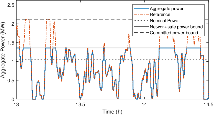
This is even more likely to happen if real-time network states differ from their forecasts and the actual network-safe bounds are tighter than those generated with the forecasts. Fig. 2 provides an example of this situation, where the dashed black lines are the power bounds obtained in advance that are used to determine the committed capacity, and the solid black lines are the actual network-safe power bounds computed in real-time. The red reference signal (a scaled and shifted frequency regulation signal from the PJM Interconnection [28]) is scaled to the committed power bounds and is impossible to track while ensuring network safety. We assume that network safety takes precedence over tracking performance, specifically, the aggregator should track the regulation signal as well as possible within the tighter bounds, i.e., the blue signal in Fig. 2. PJM uses a mechanism to constrain the integral of the normalized signal (i.e., the energy content of the signal), meaning that tracking the red signal is unlikely to cause power bound violations. However, the bound tightening in Fig. 2 makes the blue signal much harder to track; attempting to track it with a simple tracking controller would cause average aggregate power consumption to decrease from nominal, eventually rendering the signal untrackable as TCLs struggle to cool/heat sufficiently. Eventually, many TCLs may need to be on simultaneously violating the network-safe power bound. We will benchmark our approach against a simple tracking controller in Section V.
We next detail the problem formulation. We consider a collection of TCLs that are clustered into multiple groups based on their similarity in terms of thermal/electrical parameters and ambient temperatures, and we treat TCLs in the same group as homogeneous. To do this, the amount of deviations allowed between TCLs in the same group is small enough so that we can construct a bisimilar abstraction for each group; details are given in Section III-B. Our method also allows for sufficiently small process noise and variation in ambient temperature, but our mathematical development assumes no process noise and constant ambient temperature to simplify the exposition of the main results. Considering multiple groups allows us to deal with TCL heterogeneity, which we did not consider in our preliminary work [19].
Let the number of groups of homogeneous TCLs be , the total number of TCLs across all groups be , and the number of TCLs in group be ; hence, . The temperature of the th TCL in group at time is denoted by , and its domain is . Also, the on/off mode of each TCL is , which is if it is not consuming power (off), and if it is consuming power (on). Then, we assume that the temperature evolution follows the affine model developed in [29] as follows
| (1) |
Here, is the ambient temperature of TCLs in group and is , where is the sampling time, is the thermal resistance and the thermal capacitance of every TCL in group . Parameter is the thermal energy transfer rate, which is positive for a cooling TCL and negative for a heating TCL; since here we assume all TCLs are air conditioners, the value is positive. The power consumption of each TCL in group when it is in on mode, denoted , equals , where is the coefficient of performance. Then, the aggregate power consumption of all TCLs, denoted , equals .
We next define the local constraints. The temperature dead-band of group is (), which leads to the constraint
| (2) |
We assume that temperature setpoints and dead-bands are constant over time.
Additionally, a lockout constraint on every TCL requires it to remain in the same mode for a specific duration after a switch; imposing this constraint is a key extension from our preliminary work [19]. Suppose that the mode of every TCL in group should be kept for after it is turned off and for after it is turned on. Then, the number of time steps TCL should be locked after a switch for each mode is computed as
Now, let / be the last time step the th TCL in group switched its mode to off/on. Then, the input sequence should satisfy the following
| (3) | ||||
Next, we define the global constraint, which ensures the safety of the distribution network. Specifically, we bound the aggregate power consumption
| (4) |
where are the upper and lower power bounds.
Finally, our goal is to control the modes of the TCLs so that the aggregate power consumption of all TCLs tracks the reference signal as well as possible while satisfying all constraints. Then, the problem of interest is as follows.
III Abstraction and aggregation of a collection of switched subsystems
In this section, we consider an abstract problem where the goal is to coordinate a collection of switched subsystems, clustered into groups based on the similarity of their dynamics, subject to the constraints that are generalized versions of (2), (3), and (4). After we introduce this general problem setup, we explain how to construct an abstraction with discrete-states from the original continuous-state subsystems in each group. This abstraction is then used to model an “aggregate system”, representing the dynamics, which we use to synthesize a safety-guaranteed controller.
Using aggregate dynamics to represent collections of TCLs is not a new idea [10, 11, 12] but works that aim to characterize the relation between the aggregate dynamics and the actual collection are more recent. Ref. [30] abstracts a TCL as a Markov chain and probabilistically quantifies the difference between the dynamics of the underlying collection and its aggregate model. In contrast, our approach provides deterministic bounds using approximate bisimulation relations. Furthermore, their model is different because the mode of each TCL is assumed to be uncontrollable; instead their input is the temperature setpoint. Ref. [31] uses a similar approach to ours to construct abstractions and an aggregate system, but it considers continuous-time subsystems and develops open-loop control signals, whereas we consider discrete-time subsystems and propose an algorithm to compute invariant sets, which can be used to ensure safety of arbitrary feedback controllers. The abstraction and aggregation methods from our preliminary work [19] are only applicable to collections of homogeneous subsystems, whereas here we consider heterogeneous subsystems. Additionally, none of the above-mentioned approaches consider lockout constraints, as we do here.
III-A Abstract problem formulation
First, the transition systems formalism is introduced to model discrete-time dynamics [32].
Definition 1.
A transition system is a tuple , where is a set of states, a set of actions, a transition relation, and an output function.
We denote as for short.
Definition 2.
Given a transition system , a safe set , and set of admissible input constraints , a set is a controlled invariant set with respect to if and for all there exists such that for all with , we have . The union of all controlled invariant sets with respect to is called the maximal controlled invariant set for .
We consider a system that includes multiple groups of homogeneous switched subsystems. Here, the number of groups is , the number of subsystems in group is , the total number of subsystems across all groups is (i.e., ), and the number of modes is .
For any and , let be the th subsystem of group , and be its state at time step , where is a compact domain. The difference equation governing the evolution of is
| (5) |
where is the mode of th subsystem in group at time and is also the control input. For TCLs, corresponds to and corresponds to the affine dynamics in (1). For the rest of this section, we drop the index for convenience.
The discrete-time dynamics in (5) can be equivalently represented as a transition system
| (6) |
where if and only if .
To formally describe each group of subsystems, we introduce the following definition of a product transition system.
Definition 3.
Given identical copies of a transition system , the product transition system is given by , where if and only if for all ; and .
According to the definition above, group can be represented by the product transition system . Furthermore, the entire system can be represented as the product of those systems, denoted with the set of states .
Now, we introduce the constraints imposed on . First, the state of each subsystem in group should stay in the safe set (which corresponds to (2) in the TCL problem), i.e.,
| (7) |
Second, each subsystem in group cannot switch again for time steps after its mode is switched to (which corresponds to the lockout constraints (3) in the TCL problem), and so the input sequence of each subsystem should satisfy
| (8) |
where is the last time step the subsystem switched its mode to (i.e., , ). Third and finally, we impose bounds on a linear combination of the number of subsystems in each mode in each group (which corresponds to (4) in the TCL problem) as follows
| (9) |
where is a scalar corresponding to subsystems in mode in group , and is the number of subsystems in mode in group .
Additionally, we assume a time-varying cost function which depends on the number of subsystems in each mode in each group. Then, the generalized problem is as follows.
III-B Abstractions
In this section, we introduce the abstraction of each subsystem . We consider the following notion of closeness to the original subsystem.
Definition 4.
Two transition systems and are -approximately bisimilar if there exists a relation such that the sets and are non-empty for all , and such that for all , all of the following are satisfied.
- •
.
- •
If , there exists s.t. .
- •
If , there exists s.t. .
To guarantee the existence of a bisimilar abstraction for the subsystems in each group, the following assumption is made.
Assumption 1.
For every , is a local contraction, that is, there exists constants , such that
| (10) |
for every with .
This assumption holds for the temperature dynamics in (1).
Now we construct an abstraction of for every by uniformly discretizing . For a given grid size , the abstraction function is defined as
| (11) |
Suppose that the grid size for the abstraction corresponding to group is , and define the set , where is the number of elements . Then, an abstraction for is
| (12) |
where if and only if . This means that the transition relation between the states of is determined by propagating each grid point with the dynamics and finding the closest grid point to where it reaches in one time step, as shown in Fig. 3. The abstraction of each subsystem is denoted and its state is denoted . For simplicity, we drop the superscript from when not crucial.
The following lemma, a discrete-time variant of those in [33, 34], states a condition for and to be bisimilar.
Lemma 1.
If and are such that for all , then and are approximately bisimilar.
If and are -approximately bisimilar, the states of and remain -close (i.e. ) if the same input sequence is applied to both systems from the initial state , which satisfies .
By Assumption 1, we can show that, for any , there is a small enough that satisfies the condition in Lemma 1. Moreover, even when small disturbances or parameter variations exist among the subsystems in the same group, a single -approximately bisimilar system for the entire group can be constructed. In particular, for any in , let be a constant which satisfies . Then, any subsystem whose state evolution function satisfies
is also -approximately bisimilar to . This allows for mild heterogeneity within a group as long as every subsystem in it satisfies the inequality above.
The abstraction of each group can be represented by the product transition system and the abstraction of the entire system can be represented as the product of those systems, denoted , where . By definition 4, it is easy to see that and are -approximately bisimilar if and are -approximately bisimilar for all . Then, we can show the following.
Theorem 1.
Assume that and are -approximately bisimilar and is larger than . If the abstracted subsystem starting at stays inside under an input trajectory , then for every satisfying , the trajectory of starting at stays inside the safe set under .
This theorem states that, if we can obtain an input sequence for an abstracted subsystem that keeps its state inside a safe set shrunken by , then the input sequence is also safe for the original subsystem.
Using Theorem 1, we define the safe set for abstracted subsystem as and impose the following local constraints on the abstracted subsystems.
| (13) |
Fig. 3 illustrates how and its set of safe states are constructed.

Now our goal is to develop a safe control algorithm for the abstracted subsystems satisfying (13).
III-C Aggregate system
We now construct an aggregate system for each group as an alternative representation of . An aggregate system is a compact representation that keeps track of the number of subsystems in each possible combination of mode, state, and lockout duration (i.e., the number of time steps it has been locked in its current mode). The input to an aggregate system is the number of subsystems that switch mode, which can be used to determine the modes of the individual subsystems. To construct an aggregate system, we build a graph for each group that captures all possible transitions of the subsystem for all combinations of mode, state, and lockout duration. In particular, we extend the graph construction method from our preliminary work [19] by considering the lockout duration as one additional feature of a node. Then, the graph is used to express how the number of subsystems at each possible combination evolves, which acts as the dynamics of the aggregate system.
We first construct a graph for the state-abstracted subsystem , i.e., , where are the vertices and are the edges. Each node is denoted by (, , ); when is at state , in mode , and with lockout duration , we say that ‘corresponds to’ . Edges are defined for any possible autonomous or controlled transition between nodes, specifically, belongs to if and one of the following hold:
- 1.
, (system is unlocked and its mode remains unchanged),
- 2.
, , (system is locked and lockout duration is updated),
- 3.
, , (system becomes unlocked),
- 4.
, , (system is unlocked and its mode changes).
Fig. 4 illustrates how is constructed.
Now, we define the safe nodes of as the elements of the set
where is the set of indices . To abide by the local constraint for each subsystem (13), every in group should correspond to an element of .
Then, the aggregate system is constructed with state (where ), whose elements represent the number of subsystems in group corresponding to the nodes of , and input (where ), whose elements represent the number of subsystems switching mode from each node. Specifically, the element of represents the number of subsystems corresponding to and the element of represents the number of unlocked subsystems corresponding to switching mode from to . Then, the evolution of each element is governed by
| (14) |
where the set is the set of indices of the predecessors of defined as .

Since every element of evolves as a linear combination of the state and input, the dynamics of can be written as the linear dynamics
| (15) |
where and are determined by (14) and depend upon the incidence matrices of . Considering the number of subsystems in each group and the fact that only unlocked subsystems can switch mode, the state space and the admissible input space of are as follows
| (16) | ||||
Note that the lockout constraint (8) is never violated if the number of subsystems switching mode at each node is an element in the admissible input set.
The local constraint imposed on is specified by the set , defined as follows
which requires all subsystems to correspond to safe nodes.
We can also construct an alternative representation of by combining all , defined as . Accordingly, the state and input of are the concatenation of all and , respectively, which are written as , . The state space and the admissible input space are , , respectively. Then, the system dynamics of can be written as
| (17) |
where the system matrices are and . Hence, is a linear system with integer-valued state space and admissible input space. Crucially, the dimension of the state or input does not depend on the total number of subsystems .
Now, we define the set of safe states of comprising all states satisfying the local and global constraints as follows
| (18) | ||||
where the first line enforces the local constraints on all subsystems, and the second line enforces the global constraint (9); note that equals the number of the subsystems in mode . All constraints within (18) are linear inequalities.
Our objective is to develop a control algorithm for that keeps the system safe. Our algorithm, which will be introduced in Section V, incorporates a controlled invariant set to guarantee recursive safety and feasibility. However, the large dimension of makes it difficult to use existing invariant set computation tools for linear systems [31, 7, 9]. Therefore, in the next section, we propose a method that obtains an implicit representation of an invariant set of , which can be leveraged in the control algorithm.
IV Construction of an invariant set by an implicit representation
In this section, we show how to construct a controlled invariant set for the aggregate system . Leveraging the cycles of the graphs, this method finds an implicit representation of an invariant set of by identifying a set of states that can be kept inside via periodic inputs. This method is an extension of the method in our preliminary work [19] to accommodate aggregate systems with more than one group.

We first define a safe cycle as a sequence of nodes with corresponding mode sequence that satisfies if and if . Since every node of a safe cycle belongs to , if an abstracted subsystem corresponds to one of these nodes at time , then the subsystem satisfies the local constraint (13) at time . Note that at least one safe cycle should exist in each for the existence of a controlled invariant set of . Fig. 5 shows an example of a safe cycle in .
First, we introduce a strategy that uses a safe cycle to control each abstracted subsystem without violation of its local constraint (13). Consider an abstracted subsystem that corresponds to a node of the safe cycle . If we apply the mode sequence periodically to this subsystem, it visits periodically so that it never leaves . This means that if corresponds to a node of a safe cycle, applying the mode sequence of the safe cycle periodically guarantees recursive satisfaction of (13). We call this a circular shift strategy.
Next, we present a condition for recursive satisfaction of the global constraint (9) when every subsystem is controlled by a circular shift strategy. Note that (9) is a linear inequality with respect to the number of subsystems in each mode in each group. Moreover, the total number of subsystems in each mode in each group at each time is periodic since the mode of every subsystem is periodic under a circular shift strategy. This implies that, to ensure global constraint satisfaction, we only need to determine whether the maximum/minimum number of subsystems in each mode in each group within one period satisfies the global constraint. Further, these maximum/minimum values are functions of the nodes each subsystem corresponded to at the initial time step. Therefore, we can characterize an invariant set implicitly by a constraint on the initial number of subsystems corresponding to each node that guarantees the recursive satisfaction of the global constraint under a circular shift strategy.
Mathematically, we first select safe cycles from for all ; at least one safe cycle should be selected from each group (i.e., for all in ). The cycles selected from graph are denoted whose nodes are with corresponding mode sequence , where is the length of .
Next, we define the subsystem assignment of as a vector whose th element represents the number of subsystems corresponding to . Since the state of every subsystem in group corresponds to only one node at a time, the following holds
| (19) |
Next, we consider how the number of subsystems corresponding to each node changes as the subsystems are controlled by a circular shift strategy. We first define the circulant matrix as
Then, the number of subsystems at each node of after -steps of circular shift from is . Also, the number of subsystems in mode corresponding to after -steps of circular shift from is defined as
| (20) |
Note that is periodic with respect to with period because of the periodicity of .
Then, considering all selected cycles for group , the number of subsystems in mode in group after -steps of circular shift is . Hence, the global constraint (9) holds after -steps of circular shift if the following holds
| (21) |
For recursive satisfaction of the global constraint under a circular shift strategy, we need (21) to hold for all . Considering the periodicity of each with respect to , recursive satisfaction of (9) is achieved if the following two inequalities hold11 1 These two inequalities are more conservative than the constraints introduced in our preliminary work [19], yet, the number of inequalities needed is significantly less.
| (22) | ||||
| (23) |
Fig. 6 illustrates one example of subsystem assignment for each cycle that satisfies those inequalities for .

Now, a set of subsystem assignments for which the circular shift strategy never violates the given constraints can be defined as
| (24) | ||||
where is defined as .
This implies that any state of corresponding to a subsystem assignment in will always stay inside using a circular shift strategy. To obtain a set of such , we use a mapping from subsystem assignment vectors to the state of . Specifically, if , its element is
Then using this mapping, we can define the projection of into the state space of as
| (25) | |||
Therefore, the following theorem holds.
Theorem 2.
is a controlled invariant set of the system under the constraint set .
Note that the definition (25) is not an explicit representation of since we use additional variables in its description. To obtain an explicit representation that only depends on constraints in , one needs to project the implicit representation (25) to the state space . However, because of the large dimension of the set, the computational burden is large and thus the projection is usually intractable [35]. Fortunately, to check whether a state belongs to or to compute an input that guarantees invariance, an explicit representation is not necessary. Instead, if we introduce integer variables encoding the minimum/maximum in (22)-(23), can be represented with linear inequalities in , , and these integer variables, and these inequalities can be used in our formulation.
V Implicit invariant-set-driven MPC
In this section, we propose an MPC-based control algorithm with recursive safety and feasibility, referred to as Implicit Invariant-Set-Driven MPC. Suppose the state of is at time step . Then, this algorithm solves the following program at every time step for a given horizon length ,
| s.t. | (26a) | ||||
| (26b) | |||||
| (26c) | |||||
| (26d) | |||||
| (26e) | |||||
The decision variables are for all in , for all in , and for all , . The function is the cost with respect to the state of corresponding to in Problem 2. In (26d), is a vector with the entries of corresponding to group . After solving this problem, we select the optimal as the input which drives the state to .
To guarantee recursive safety and feasibility, this algorithm uses a similar scheme to those introduced in [4, 5, 6], in which the state at the end of the horizon is required to belong to an invariant set. However, instead of using an explicit representation, our algorithm uses the obtained implicit representation to formulate the constraint (26d).
Theorem 3.
Suppose that the initial state belongs to the -step backward reachable set of . Then, the program (26) has a feasible solution at any time step . In addition, the trajectory generated by the algorithm always belongs to the maximal controlled invariant set of , and therefore belongs to , for every .
Since the proof of this theorem is similar to the one of Theorems III.5. and III.7. of [5], we do not provide it here.
Remark 1.
The performance of implicit invariant-set-driven MPC in terms of cost minimization becomes better as the size of and the length of horizon increases, and the size of usually increases when the number of cycles selected from is larger. However, more cycles and larger mean more variables and constraints, requiring more computation time. Thus, and should be carefully chosen considering this trade-off.
To implement the control input, we arbitrarily select out of unlocked subsystems in mode and state (i.e., subsystems corresponding to node ) and switch their mode to . This process is repeated for all . The state of each subsystem at each time step can be determined from the sequence of states and inputs obtained by implicit invariant-set-driven MPC.
By Theorems 1 and 3, this switching control approach guarantees always satisfies the constraints (7),(8),(9). First, the lockout constraint (8) is never violated since the controller only switches unlocked subsystems. Second, the global constraint (9) holds by Theorem 3; the obtained state trajectory always belongs to . Third and finally, the local constraint (7) holds because every subsystem corresponds to one of the nodes in , i.e, state always belongs to , and so, by Theorem 1, the state trajectory of each always belongs to .
VI Simulation Results
In this section, we compare the performance of implicit invariant-set-driven MPC to several benchmark algorithms by solving Problem 1. We assume that two groups of homogeneous TCLs (i.e. ) are connected to the 56-bus balanced distribution network in [36]. 22 2 The parameters used are as follows: °C, kWh/°C, kWh/°C, °C/kW, °C/kW, kW, kW, °C, °C, °C, °C, , , s, s. The uncontrollable load at each node is assumed to be constant with the value of 50% of the nominal power consumption at each node; the other 50% is the nominal power consumption of controllable TCLs. We use a time discretization of the TCL dynamics of s.
For the safety of the network, we try to prevent under-voltages, where the lower bound on voltage is set to 0.95 p.u.. From this bound on voltage, the safe upper bound on aggregate power is obtained using the method proposed in [21]. Note that our preliminary work [19] did not explicitly consider a network model, or show the impact of TCL control on the network, like we do here.
The reference signal for aggregate TCLs is obtained by shifting and scaling a PJM frequency regulation signal [28] from 13:00 to 14:30. We both shift and scale it by the nominal power consumption of the controllable TCLs. The cost function to measure the tracking performance is
| (27) |
The number of cycles selected for implicit invariant-set-driven MPC for each group is . The parameters for the abstraction are , , , and . Gurobi is used to solve the optimization problems, and the limitation on the solve time of each iteration of MPC is set to 1000s; if the solver cannot find an optimal solution in 1000s, a suboptimal solution is used.
VI-A Benchmark algorithms
Three benchmark algorithms are compared with implicit invariant-set-driven MPC.
VI-A1 Benchmark 1
This MPC algorithm requires the states to be inside over the optimization horizon. The problem solved at time is
When this problem is feasible, the obtained solution keeps the state inside . However, this algorithm does not ensure recursive feasibility. Therefore, the state may go outside of the maximal controlled invariant set and the problem may become infeasible.
VI-A2 Benchmark 2
Instead of imposing a constraint for safety, this MPC algorithm tracks the reference signal truncated between the aggregate power limits (the blue line in Fig. 2). The truncated reference signal is
Then, the problem solved at time is
| s.t. |
Since this problem has fewer constraints, the computational burden of this algorithm is less than that of the others. However, solutions from this algorithm may violate the aggregate power limits if is not perfectly tracked.
VI-A3 Benchmark 3
The third benchmark is a version of invariant-set-driven MPC introduced in our preliminary work [19], which does not consider lockout constraints.
Note that Benchmarks 1 and 2 use the same aggregate system as implicit invariant-set-driven MPC, while Benchmark 3 leverages an aggregate system introduced in [19], whose state does not include locked durations.
VI-B Numerical Experiments
VI-B1 Experiment 1
We first verify the recursive feasibility of implicit invariant-set-driven MPC in contrast to Benchmark 1. Fig. 7 shows the results of Benchmark 1 and implicit invariant-set-driven MPC. Neither algorithm violates the bounds on aggregate power. Benchmark 1 shows better tracking performance at first. However, to achieve this, the temperatures of many of the TCLs in off-mode increase towards the upper bounds of their dead-bands. Eventually, no input exists that satisfies both the temperature and aggregate power constraints at the next time step. Thus, the problem becomes infeasible around 13.25h. In contrast, even though, initially, implicit invariant-set-driven MPC has worse tracking performance, it ensures feasibility at any time step by turning on some TCLs in advance.


VI-B2 Experiment 2
In this experiment, we compare Benchmarks 2 and 3 with implicit invariant-set-driven MPC in terms of both tracking performance and constraint satisfaction. The results are shown in Fig. 8 and Table I. Benchmark 2 has the best tracking performance, but the aggregate power exceeds the upper bound around 13.8h and 14.1h. Benchmark 3 never violates the bounds on aggregate power, but it makes an average of 12% of TCLs violate their lockout constraints at each time step. In contrast, implicit invariant-set-driven MPC never violates the aggregate power or lockout constraints.
The plots at the bottom of Fig. 8 show the voltage at every node in the network for each algorithm. We see that Benchmark 2 leads to an under-voltage violation when the bound on aggregate power is violated. In contrast, Benchmark 3 and implicit invariant-set-driven MPC maintain safe voltages across the network. We note that the particular voltage violation seen in Fig. 8 is small and unlikely to cause a real issue in the network, but other combinations of tracking signals, aggregate power bounds, and networks could lead to more severe violations that our approach would guard against.
The average time expended for each iteration of MPC is presented in Table I. Each iteration of implicit invariant-set-driven MPC takes much longer than that of Benchmark 2. Note that the average value exceeds the sampling time . This means that the current implementation of the algorithm cannot be leveraged online and thus reducing the computation burden is an important topic for future work.


VII Conclusions
In this paper, we proposed an invariant set construction method that provides an implicit representation of the safe set of a system of heterogeneous switched subsystems with both local and global safety constraints. This representation is incorporated, via a terminal condition, into our proposed MPC-based control algorithm. Since the computational burden of this algorithm is independent of the number of subsystems, it is scalable to large collections of subsystems. Numerical simulation results demonstrated the safety and recursive feasibility of the approach.
Possible future work includes the development of data-driven abstractions to allow for more heterogeneity. From an application-domain standpoint, it would also be valuable to develop approaches that handle time-varying power bounds, temperature setpoints, ambient temperatures, and disturbances.
References
- [1] D. Bertsekas, “Infinite time reachability of state-space regions by using feedback control,” IEEE Trans. Automat. Contr., vol. 17, no. 5, pp. 604–613, 1972.
- [2] J.-P. Aubin, A. Bayen, and P. Saint-Pierre, Viability theory: new directions. Springer Science & Business Media, 2011.
- [3] F. Blanchini, “Set invariance in control,” Automatica, vol. 35, no. 11, pp. 1747–1767, 1999.
- [4] T. Koller, F. Berkenkamp, M. Turchetta, and A. Krause, “Learning-based model predictive control for safe exploration,” in Proc. IEEE Conf. Decis. Control, 2018, pp. 6059–6066.
- [5] K. P. Wabersich and M. N. Zeilinger, “Linear model predictive safety certification for learning-based control,” in Proc. IEEE Conf. Decis. Control, 2018, pp. 7130–7135.
- [6] K. P. Wabersich, L. Hewing, A. Carron, and M. N. Zeilinger, “Probabilistic model predictive safety certification for learning-based control,” IEEE Trans. Automat. Contr., vol. 67, no. 1, pp. 176–188, 2021.
- [7] T. Anevlavis and P. Tabuada, “Computing controlled invariant sets in two moves,” in Proc. IEEE Conf. Decis. Control, 2019, pp. 6248–6254.
- [8] M. Fiacchini and M. Alamir, “Computing control invariant sets in high dimension is easy,” arXiv:1810.10372, 2018.
- [9] A. Wintenberg and N. Ozay, “Implicit invariant sets for high-dimensional switched affine systems,” in Proc. IEEE Conf. Decis. Control, 2020, pp. 3291–3297.
- [10] J. Mathieu, S. Koch, and D. Callaway, “State estimation and control of electric loads to manage real-time energy imbalance,” IEEE Trans. Power Syst., vol. 28, no. 1, pp. 430–440, 2012.
- [11] S. Bashash and H. K. Fathy, “Modeling and control of aggregate air conditioning loads for robust renewable power management,” IEEE Trans. Control Syst. Technol., vol. 21, no. 4, pp. 1318–1327, 2012.
- [12] W. Zhang, J. Lian, C.-Y. Chang, and K. Kalsi, “Aggregated modeling and control of air conditioning loads for demand response,” IEEE Trans. Power Syst., vol. 28, no. 4, pp. 4655–4664, 2013.
- [13] S. Tindemans, V. Trovato, and G. Strbac, “Decentralized control of thermostatic loads for flexible demand response,” IEEE Trans. Control Syst. Technol., vol. 23, no. 5, pp. 1685–1700, 2015.
- [14] A. Coffman, N. Cammardella, P. Barooah, and S. Meyn, “Aggregate capacity of TCLs with cycling constraints,” arXiv:1909.11497, 2019.
- [15] C. Ziras, S. You, H. W. Bindner, and E. Vrettos, “A new method for handling lockout constraints on controlled TCL aggregations,” in Power Syst. Comput. Conf., 2018.
- [16] E. Dall’Anese, S. Guggilam, A. Simonetto, Y. C. Chen, and S. Dhople, “Optimal regulation of virtual power plants,” IEEE Trans. on Power Syst., vol. 33, no. 2, pp. 1868–1881, 2017.
- [17] A. Bernstein and E. Dall’Anese, “Real-time feedback-based optimization of distribution grids: A unified approach,” IEEE Trans. Control Netw. Syst., vol. 6, no. 3, pp. 1197–1209, 2019.
- [18] E. Vrettos and G. Andersson, “Combined load frequency control and active distribution network management with thermostatically controlled loads,” in IEEE SmartGridComm, 2013, pp. 247–252.
- [19] S. Jang, N. Ozay, and J. L. Mathieu, “Large-scale invariant sets for safe coordination of thermostatic loads,” in Proc. Amer. Ctrl. Conf., 2021, pp. 4163–4170.
- [20] S. Ross, G. Vuylsteke, and J. Mathieu, “Effects of load-based frequency regulation on distribution network operation,” IEEE Trans. Power Syst., vol. 34, no. 2, pp. 1569–1578, 2019.
- [21] S. C. Ross and J. L. Mathieu, “A method for ensuring a load aggregator’s power deviations are safe for distribution networks,” Electr. Power Syst. Res., vol. 189, p. 106781, 2020.
- [22] N. Nazir and M. Almassalkhi, “Convex inner approximation of the feeder hosting capacity limits on dispatchable demand,” in Proc. IEEE Conf. Decis. Control, 2019, pp. 4858–4864.
- [23] D. Molzahn and L. Roald, “Grid-aware versus grid-agnostic distribution system control: A method for certifying engineering constraint satisfaction,” in HICSS, 2019, pp. 3445–3454.
- [24] B. Cui, A. Zamzam, and A. Bernstein, “Network-cognizant time-coupled aggregate flexibility of distribution systems under uncertainties,” in Proc. Amer. Ctrl. Conf., 2021, pp. 4178–4183.
- [25] S. Ross, N. Ozay, and J. Mathieu, “Coordination between an aggregator and distribution operator to achieve network-aware load control,” in IEEE Milan PowerTech, 2019.
- [26] PJM, “Implementation and rationale for PJM’s conditional neutrality regulation signals,” 2017, [Online]. Available: https://www.pjm.com//media/committees-groups/task-forces/rmistf/postings/regulation-market-whitepaper.ashx.
- [27] CAISO, “Non-generator resource (NGR) and regulation energy management (REM) overview - phase 1,” 2014, [Online]. Available:https://www.caiso.com/documents/ngr-removerview.pdf.
- [28] PJM, “RTO regulation signal data for 7.19.2019 & 7.20.2019.xls,” https://www.pjm.com/markets-and-operations/ancillary-services.aspx, accessed: 2019-10-22.
- [29] R. C. Sonderegger, Dynamic models of house heating based on equivalent thermal parameters. Ph.D. dissertation, Princeton University, 1978.
- [30] S. E. Z. Soudjani and A. Abate, “Aggregation and control of populations of thermostatically controlled loads by formal abstractions,” IEEE Trans. Control Syst. Technol., vol. 23, no. 3, pp. 975–990, 2014.
- [31] P. Nilsson and N. Ozay, “Control synthesis for permutation-symmetric high-dimensional systems with counting constraints,” IEEE Trans. Automat. Contr., vol. 65, no. 2, pp. 461–476, 2019.
- [32] P. Tabuada, Verification and control of hybrid systems: a symbolic approach. Springer Science & Business Media, 2009.
- [33] G. Pola and P. Tabuada, “Symbolic models for nonlinear control systems: Alternating approximate bisimulations,” SIAM J. Control Optim., vol. 48, no. 2, pp. 719–733, 2009.
- [34] P. Nilsson and N. Ozay, “Control synthesis for large collections of systems with mode-counting constraints,” in Proc. ACM Int. Conf. Hybrid Syst.: Comput. Control, 2016, pp. 205–214.
- [35] H. Tiwary, “On the Hardness of Computing Intersection, Union and Minkowski Sum of Polytopes,” Discrete Comput. Geom., vol. 40, no. 3, pp. 469–479, 2008.
- [36] S. Bolognani and S. Zampieri, “On the existence and linear approximation of the power flow solution in power distribution networks,” IEEE Trans. Power Syst., vol. 31, no. 1, pp. 163–172, 2015.
Appendix
Supplements & Proofs for Section III :
Lemma 1.
It follows from [34] where acts as the class -function in their proof for a fixed sampling time. ∎
The following lemma is used to prove Theorem 1.
Lemma 2.
If holds, is a subset of .
Proof.
First, the abstraction function satisfies from which we obtain
Also, we have
where the first equation uses the definition of the Minkowski sum, and the second relationship between the sets comes from . Since is the largest set in that satisfies , the following holds,
and the statement has been proven. ∎
Theorem 1.
Let be larger than . From the statement of the Theorem, the following holds
| (28) |
Proofs for Section IV :
Theorem 2.
We first show that is a subset of . Let be an element of . By the definition of , there exists a vector such that for all in . Then, for any , we can show
| (29) |
since all the nodes belong to .
Also, the following equation holds,
Therefore, we obtain the following
| (30) |
From (21) and (30), the following holds
| (31) |
Next, we show the recurrence property of . Let be the input corresponding to 1-step of circular shift from , and be the corresponding next state from under (i.e., ). Then, is equal to for any in . To show that is an element of , we show that belongs to .