Many-Body Quantum Muon Effects and Quadrupolar Coupling in SolidsPreprint: APS/123-QED

Within the classical, point-particle description of muons and nuclei using DFT, we find a single stable muon site at almost exactly the $(0,1/4,1/4)$ position (Fig. 1b and Supplementary Fig. 1b), which lies between two molecules of pristine $\alpha$–$\text{N}{\vphantom{\text{X}}}_{\smash[t]{\text{2}}}$ but is not symmetric under its $Pa\bar{3}$ space group ^{41; 42}. In line with ab initio simulations of muons ³⁶ and protons ^{43; 44; 45; 46; 47} in $\text{N}{\vphantom{\text{X}}}_{\smash[t]{\text{2}}}$ clusters, we find that in crystalline $\alpha$–$\text{N}{\vphantom{\text{X}}}_{\smash[t]{\text{2}}}$ a muon forms an almost-linear, almost-centrosymmetric $\text{[}\text{N}{\vphantom{\text{X}}}_{\smash[t]{\text{2}}}\text{\hskip 1.29167pt--\hskip 1.29167pt}\text{\text{$\mu$ }}\text{\hskip 1.29167pt--\hskip 1.29167pt}\text{N}{\vphantom{\text{X}}}_{\smash[t]{\text{2}}}\text{]}\text{}{\vphantom{\text{X}}}^{\text{+}}$ complex oriented along the $[0,1,1]$ direction. Within this complex the muon’s bare positive charge $+e_{0}$ is screened to just $+0.46e_{0}$ by electrons covalently shared with the two nearest $\text{N}{\vphantom{\text{X}}}_{\smash[t]{\text{2}}}$ molecules, leaving them with an electron density deficit and thus a net positive charge of $+0.27e_{0}$ each ($+0.04e_{0}$ on the two nearest N atoms and $+0.23e_{0}$ on the two further-away ones; Fig. 1b and Supplementary Fig. 2). Moreover, we find that an unusual, extended electric-dipole polaron forms around this complex, where its positive charge further induces electric dipole moments (Fig. 1c) on other, net neutral nearby $\text{N}{\vphantom{\text{X}}}_{\smash[t]{\text{2}}}$ molecules (Supplementary Fig. 2) and causes them to reorient to point towards the complex. Up to $\sim 4\text{\,}\mathrm{\SIUnitSymbolAngstrom}$ from the muon, dipolar electrostatic interactions of polarized $\text{N}{\vphantom{\text{X}}}_{\smash[t]{\text{2}}}$ molecules with the $\text{[}\text{N}{\vphantom{\text{X}}}_{\smash[t]{\text{2}}}\text{\hskip 1.29167pt--\hskip 1.29167pt}\text{\text{$\mu$ }}\text{\hskip 1.29167pt--\hskip 1.29167pt}\text{N}{\vphantom{\text{X}}}_{\smash[t]{\text{2}}}\text{]}\text{}{\vphantom{\text{X}}}^{\text{+}}$ complex thus overwhelm the weak electric quadrupole and van der Waals (VdW) $\text{N}{\vphantom{\text{X}}}_{\smash[t]{\text{2}}}$–$\text{N}{\vphantom{\text{X}}}_{\smash[t]{\text{2}}}$ interactions of pristine $\alpha$–$\text{N}{\vphantom{\text{X}}}_{\smash[t]{\text{2}}}$ ^{40; 48}.

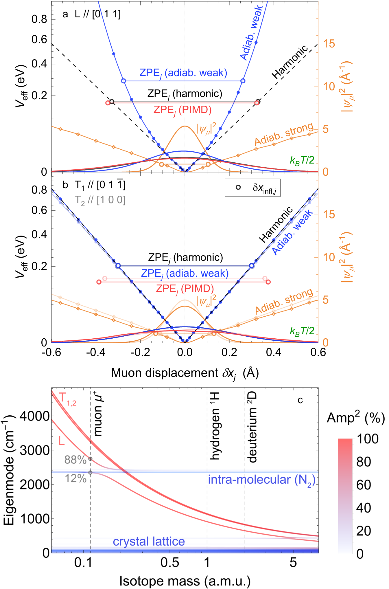
To incorporate quantum effects we first employ single-particle, adiabatic approximations of muon–nuclear ZPM. Though elaborate schemes have been proposed ^{22; 29}, the simplest are weakly- and strongly-bound muon approximations ^{26; 27; 28}, corresponding to zero or maximal muon–nuclear entanglement, respectively. In both schemes, an effective single-particle muon potential $V_{\mathrm{eff}}({\bm{\mathbf{\delta x}}})$ is constructed from total DFT energy under muon displacements ${\bm{\mathbf{\delta x}}}$ from its classical site, while: (i) keeping the nuclei fixed at the positions corresponding to the unperturbed muon site (weakly-bound case), or (ii) letting them relax by ${\bm{\mathbf{\delta\widetilde{r}}}}_{\mathrm{N}}({\bm{\mathbf{\delta x}}})$ to new lowest-energy positions for each ${\bm{\mathbf{\delta x}}}$ (strongly-bound case) while keeping the center of mass fixed. Respectively, this corresponds to: (i) assuming independent muon and nuclear ZPM [i.e., a separable muon–nuclear wavefunction, $\psi({\bm{\mathbf{\delta x}}},{\bm{\mathbf{\delta r}}}_{\mathrm{N}})=\psi_{\mu}({\bm{\mathbf{\delta x}}})\psi_{\mathrm{N}}({\bm{\mathbf{\delta r}}}_{\mathrm{N}})$] in the weakly-bound case, or (ii) ZPM where a quantum measurement of the muon displacement ${\bm{\mathbf{\delta x}}}$ would simultaneously also determine all nuclear displacements ${\bm{\mathbf{\delta r}}}_{\mathrm{N}}$ [i.e., a maximally-entangled muon–nuclear wavefunction, $\psi({\bm{\mathbf{\delta x}}},{\bm{\mathbf{\delta r}}}_{\mathrm{N}})\propto\psi_{\mu}({\bm{\mathbf{\delta x}}})\delta({\bm{\mathbf{\delta r}}}_{\mathrm{N}}-{\bm{\mathbf{\delta\widetilde{r}}}}_{\mathrm{N}}({\bm{\mathbf{\delta x}}}))$, where $\delta$ is the Dirac delta function] in the strongly-bound case. Although, by the variational principle, the strongly-bound potential is shallower than the weakly-bound potential (which would tend to increase muon delocalization), the effective mass $m_{\mathrm{eff}}$ in the strongly-bound case increases above the free-muon mass $m_{\mu}$ due to additional movement of nuclei with the muon (which would tend to decrease muon delocalization), meaning that muon ZPM delocalization can either increase or decrease in the strongly-bound case. Explicitly, assuming a linear dependence of the displacement of the $i$th nucleus of mass $m_{i}$ on the muon displacement, i.e., ${\bm{\mathbf{\delta\widetilde{r}}}}_{\mathrm{N}i}({\bm{\mathbf{\delta x}}})=A_{i}{\bm{\mathbf{\delta x}}}$ where $A_{i}$ is a tensor, the effective mass tensor in the strongly-bound case is given by $m_{\mathrm{eff}}=m_{\mu}\mathrm{id}+\sum_{i}m_{i}A_{i}^{\mathrm{T}}A_{i}$ where $\mathrm{id}$ is the identity tensor. In the weakly-bound case, $m_{\mathrm{eff}}=m_{\mu}$. Once $V_{\mathrm{eff}}({\bm{\mathbf{\delta x}}})$ and $m_{\mathrm{eff}}$ are known, a single-particle Schrödinger equation for the muon wavefunction $\psi_{\mu}({\bm{\mathbf{\delta x}}})$, $[-\hbar^{2}/(2m_{\mathrm{eff}})]\nabla^{2}\psi_{\mu}+V_{\mathrm{eff}}\psi_{\mu}=(\mathrm{ZPE})\psi_{\mu}$, can be numerically solved to obtain the muon–nuclear ZPM, encoded in $\psi_{\mu}({\bm{\mathbf{\delta x}}})$, and the corresponding ZPE. This inherently single-particle approximation with 3 degrees of freedom in ${\bm{\mathbf{\delta x}}}$ (due to the assumed zero or maximal muon–nuclear entanglement) cannot describe many-body ZPM involving more than 3 degrees of freedom (i.e., cases with partial muon–nuclear entanglement).

Fig. 2a, b show the calculated weakly- and strongly-bound adiabatic effective potentials. Separable potentials are assumed with one eigenaxis, $\mathrm{L}\parallel[0,1,1]$, along the $\text{[}\text{N}{\vphantom{\text{X}}}_{\smash[t]{\text{2}}}\text{\hskip 1.29167pt--\hskip 1.29167pt}\text{\text{$\mu$ }}\text{\hskip 1.29167pt--\hskip 1.29167pt}\text{N}{\vphantom{\text{X}}}_{\smash[t]{\text{2}}}\text{]}\text{}{\vphantom{\text{X}}}^{\text{+}}$ complex and two, $\mathrm{T}_{1}\parallel[0,1,\bar{1}]$ and $\mathrm{T}_{2}\parallel[0,0,1]$, transverse to it, coinciding with muon $\Gamma$-point normal mode directions from DFT (Fig. 2c). Table 1 lists the total muon $\mathrm{ZPE}=\sum_{j}\mathrm{ZPE}_{j}$ with directional contribution $\mathrm{ZPE}_{j}$ and muon wavefunction widths ${\Delta x}_{j}=\braket{{\delta x}_{j}^{2}}^{1/2}$ along the $j=\mathrm{L}$, $\mathrm{T}_{1}$, and $\mathrm{T}_{2}$ directions under both approximations. In the weakly-bound case, we find muon ZPM delocalization of $0.16$–$0.20\text{\,}\mathrm{\SIUnitSymbolAngstrom}$, which is significant compared to the $1.29(1)\text{\,}\mathrm{\SIUnitSymbolAngstrom}$ distance between the classical muon site and the nearest nitrogen. However, in the strongly-bound case we also find large directional effective muon mass renormalization $m_{\mathrm{eff},j}/m_{\mu}$ due to strong electrostatic interactions within the $\text{[}\text{N}{\vphantom{\text{X}}}_{\smash[t]{\text{2}}}\text{\hskip 1.29167pt--\hskip 1.29167pt}\text{\text{$\mu$ }}\text{\hskip 1.29167pt--\hskip 1.29167pt}\text{N}{\vphantom{\text{X}}}_{\smash[t]{\text{2}}}\text{]}\text{}{\vphantom{\text{X}}}^{\text{+}}$ complex and with the surrounding polaron, which leads to a large number of nitrogen nuclei following the displaced muon (up to $494m_{\mu}$ in the complex and a further $494m_{\mu}$ just in first shell of the polaron). This leads to a significantly reduced $\mathrm{ZPE}$ and delocalization (Table 1) under the strongly-bound approximation, despite a shallower effective potential (Fig. 2a, b) compared to the weakly-bound case.

Given the discrepancy between the two adiabatic approximations, the question of their applicability arises. In other words, whether muon–nuclear ZPM is minimally (weakly-bound limit), maximally (strongly-bound limit), or partially entangled. We address this using a toy model with the muon bound to $N=2$ nearby effective nuclei with force constants $k_{\mu}$, which are further bound to a static lattice with force constants $k_{\mathrm{n}}$. If $k_{\mu}\ll k_{\mathrm{n}}$ muon displacements barely perturb the nuclei (weakly-bound limit), while if $k_{\mu}\gg k_{\mathrm{n}}$ muon displacements strongly displace nearby nuclei (strongly-bound limit). We estimate the ratio $k_{\mu}/k_{\mathrm{n}}$ in $\alpha$–$\text{N}{\vphantom{\text{X}}}_{\smash[t]{\text{2}}}$ from the ratio of adiabatic potentials as $k_{\mu,j}/k_{\mathrm{n},j}=V_{\mathrm{eff}}^{\mathrm{weak}}/V_{\mathrm{eff}}^{\mathrm{strong}}-1\approx 7$, $12$, and $9$ along the $j=\mathrm{L}$, $\mathrm{T}_{1}$, and $\mathrm{T}_{2}$ directions, respectively (Fig. 2a, b). This excludes the weakly- but not the strongly-bound adiabatic approximation. However, the relatively large ratio $k_{\mu}/k_{\mathrm{n}}$ still competes with the tendency of light particles to partially positionally decouple from heavier particles ²³, which could lead to an intermediate, partially-entangled regime where single-particle (adiabatic) approximations fail. This is tendency is expected to be further reinforced by the enhanced mass $m_{\mathrm{n},j}$ of effective nearest nuclei in the toy model needed to obtain the same calculated effective muon mass $m_{\mathrm{eff},j}$ under the strongly-bound adiabatic approximation both from DFT (Table 1) and from the toy model. Namely, in the toy model we need $m_{\mathrm{n},j}=(1+k_{\mathrm{n},j}/k_{\mu,j})^{2}(m_{\mathrm{eff},j}-m_{\mu})/N=4.2(9)m_{\mathrm{N}}$, $1.7(2)m_{\mathrm{N}}$, and $2.6(4)m_{\mathrm{N}}$ along the $j=\mathrm{L}$, $\mathrm{T}_{1}$, and $\mathrm{T}_{2}$ directions, respectively, where $m_{\mathrm{N}}$ is the mass of a nitrogen nucleus.

An alternative class of approximations are harmonic methods ^{30; 31; 20}, which work in the many-body regime of partial entanglement, but are limited to strictly harmonic muon–nuclear interactions. These start with a $\Gamma$-point DFT phonon calculation in the classical muon site geometry (a muon is a localized defect and thus has no $q$-space dispersion). The usual assumption that, since muons are lighter than nuclei, muon ZPM is fully adiabatically decoupled from the lattice (yielding 3 highest-frequency normal modes $\omega_{j}$ describing single-particle muon ZPM; see Fig. 2c), corresponds to the weakly-bound (zero entanglement) adiabatic limit described above, but with the additional constraint of a harmonic adiabatic potential $V_{\mathrm{eff}}$. This assumption yields directional ZPE contributions $\mathrm{ZPE}_{j}=\hbar\omega_{j}/2$ and directional ZPM delocalization ${\Delta x}_{j}=\sqrt{\hbar/(2m_{\mu}\omega_{j})}$. The $>40\text{\,}\mathrm{\%}$ discrepancy between the harmonic and anharmonic weakly-bound adiabatic values of ${\Delta x}_{\mathrm{L}}$ thus obtained (Table 1) hints at a breakdown of the harmonic approximation due to strong anharmonicity (Fig. 2a).

Although the weakly-bound adiabatic limit is exact if $m_{\mu}\rightarrow 0$, it cannot reproduce non-zero muon–nuclear entanglement. In fact, in $\alpha$–$\text{N}{\vphantom{\text{X}}}_{\smash[t]{\text{2}}}$ we see strong hybridization of the $\mathrm{L}$ muon normal mode with intra-molecular vibrations of both $\text{N}{\vphantom{\text{X}}}_{\smash[t]{\text{2}}}$ molecules in the $\text{[}\text{N}{\vphantom{\text{X}}}_{\smash[t]{\text{2}}}\text{\hskip 1.29167pt--\hskip 1.29167pt}\text{\text{$\mu$ }}\text{\hskip 1.29167pt--\hskip 1.29167pt}\text{N}{\vphantom{\text{X}}}_{\smash[t]{\text{2}}}\text{]}\text{}{\vphantom{\text{X}}}^{\text{+}}$ complex due to a finite muon mass (Fig. 2c), which implies significant muon–nuclear entanglement ^{49; 50}. This is detected by projecting the top 3 (normalized) phonon normal modes onto pure muon motion, summing the squared norms of the resulting (projected) phonon eigenvectors, and subtracting the value $3$, which is expected when muon normal modes do not mix with the lattice modes (i.e., in the weakly-bound limit). This defines an entanglement witness ^{33; 34; 35} $w_{1}$ as $w_{1}=0$ for zero muon–nuclear entanglement (weakly-bound adiabatic limit) and $w_{1}<0$ in the entangled, many-body case. For muons in $\alpha$–$\text{N}{\vphantom{\text{X}}}_{\smash[t]{\text{2}}}$ we obtain $w_{1}=-0.14<0$. This again suggests that the weakly- (and possibly also the strongly-) bound adiabatic approximation should fail, as muon–nuclear ZPM is inherently many-body, at least in the harmonic approximation. Were it not for strong anharmonicity, which invalidates the approach, such complex ZPM could still be treated by the full, many-body harmonic method by considering the entire supercell $\Gamma$-point phonon spectrum.

Finally, we turn to numerically-exact PIMD for calculating observables from arbitrary muon–nuclear ZPM ^{1; 2; 3}, based on discretizing imaginary-time, $T>0$, path integrals. Unlike approximate methods, PIMD works even in the anharmonic many-body regime with partial muon–nuclear entanglement ⁵¹. Using PIMD we find that the projected muon probability density is unimodal in $\alpha$–$\text{N}{\vphantom{\text{X}}}_{\smash[t]{\text{2}}}$ (Fig. 2a, b), confirming that the muon site is unique even for quantum muons ⁴⁴, with no signs of quantum tunneling. Thoroughly testing PIMD convergence of observables against simplified toy-model simulations, we confirm that all observables are well converged by $P=16$–$24$ PIMD beads (imaginary-time steps), except for muon ZPM delocalization ${\Delta x}_{j}$, where we can correct for finite-$P$ effects via a careful $P\rightarrow\infty$ extrapolation scheme (see Methods and Figs. S3 and S4). We find that muon ${\Delta x}_{\mathrm{L}}$ is large enough (Table 1) that anharmonic effects become significant (Fig. 2a) and harmonic approximations fail. Furthermore, all ${\Delta x}_{j}$ are larger than in the weakly- and strongly-bound adiabatic approximations, implying partial muon–nuclear entanglement and many-body ZPM outside of the scope of single-particle approximations, as already anticipated from $\mathrm{L}$ normal mode hybridization (Fig. 2c). To quantify the degree of entanglement we calculate a multivariate Pearson correlation coefficient ⁵²

between the centered muon displacement ${\bm{\mathbf{\delta x}}}^{\prime}={\bm{\mathbf{\delta x}}}-\braket{{\bm{\mathbf{\delta x}}}}$ and the centered displacement ${\bm{\mathbf{\delta r}}}_{\mathrm{N}i}^{\prime}={\bm{\mathbf{\delta r}}}_{\mathrm{N}i}-\braket{{\bm{\mathbf{\delta r}}}_{\mathrm{N}i}}$ of a nucleus $i$, via PIMD. The quantity $w_{2i}=-|c_{i}|\in[-1,0]$ is a witness of muon–nuclear entanglement ^{33; 34; 35}, since $w_{2i}=0$ for separable (weakly-bound) states (as then $\braket{{\bm{\mathbf{\delta x}}}^{\prime}\cdot{\bm{\mathbf{\delta r}}}_{\mathrm{N}i}^{\prime}}=\braket{{\bm{\mathbf{\delta x}}}^{\prime}}\cdot\braket{{\bm{\mathbf{\delta r}}}_{\mathrm{N}i}^{\prime}}=0$), which means that $w_{2i}<0$ implies entanglement. On the other hand, in the strongly-bound case (maximal entanglement) with ${\bm{\mathbf{\delta\widetilde{r}}}}_{\mathrm{N}i}\propto{\bm{\mathbf{\delta x}}}$ we find $|c_{i}|=$100\text{\,}\mathrm{\%}$$. In $\alpha$–$\text{N}{\vphantom{\text{X}}}_{\smash[t]{\text{2}}}$ the degree of muon–nuclear entanglement is $c_{i}\approx$30(4)\text{\,}\mathrm{\%}$$ with the two nearest nitrogen nuclei, and decays with distance (Fig. 1c). This confirms that muon–nuclear ZPM in $\alpha$–$\text{N}{\vphantom{\text{X}}}_{\smash[t]{\text{2}}}$ is partially entangled and thus inherently many-body. We note that a many-body harmonic approximation calculation ^{50; 29} would yield a similar $c_{i}$ (${\approx}$26\text{\,}\mathrm{\%}$$) between the muon and the two nearest nitrogen nuclei.

Detailed knowledge of the many-body muon–nuclear ZPM afforded by PIMD allows us to derive an important constant: the static NQCC of $\hphantom{{}^{\text{14}}_{\text{}}}{\vphantom{\text{X}}}{}^{\mathchoice{\hbox to0.0pt{\hss$\displaystyle\vphantom{\smash[t]{\text{2}}}\text{14}$}}{\hbox to0.0pt{\hss$\textstyle\vphantom{\smash[t]{\text{2}}}\text{14}$}}{\hbox to0.0pt{\hss$\scriptstyle\vphantom{\smash[t]{\text{2}}}\text{14}$}}{\hbox to0.0pt{\hss$\scriptscriptstyle\vphantom{\smash[t]{\text{2}}}\text{14}$}}}\kern 0.0pt\text{N}$ in $\alpha$–$\text{N}{\vphantom{\text{X}}}_{\smash[t]{\text{2}}}$, defined as $C_{\mathrm{Q}}^{0}=e_{0}^{2}q_{0}Q/h$, where $Q=$2.044(3)\text{\,}{\mathrm{fm}}^{2}$$ is the quadrupolar moment of $\hphantom{{}^{\text{14}}_{\text{}}}{\vphantom{\text{X}}}{}^{\mathchoice{\hbox to0.0pt{\hss$\displaystyle\vphantom{\smash[t]{\text{2}}}\text{14}$}}{\hbox to0.0pt{\hss$\textstyle\vphantom{\smash[t]{\text{2}}}\text{14}$}}{\hbox to0.0pt{\hss$\scriptstyle\vphantom{\smash[t]{\text{2}}}\text{14}$}}{\hbox to0.0pt{\hss$\scriptscriptstyle\vphantom{\smash[t]{\text{2}}}\text{14}$}}}\kern 0.0pt\text{N}$ ^{53; 42}, and $q_{0}$ is the largest eigenvalue of the electric field gradient (EFG) eigenvalue at the $\hphantom{{}^{\text{14}}_{\text{}}}{\vphantom{\text{X}}}{}^{\mathchoice{\hbox to0.0pt{\hss$\displaystyle\vphantom{\smash[t]{\text{2}}}\text{14}$}}{\hbox to0.0pt{\hss$\textstyle\vphantom{\smash[t]{\text{2}}}\text{14}$}}{\hbox to0.0pt{\hss$\scriptstyle\vphantom{\smash[t]{\text{2}}}\text{14}$}}{\hbox to0.0pt{\hss$\scriptscriptstyle\vphantom{\smash[t]{\text{2}}}\text{14}$}}}\kern 0.0pt\text{N}$ position, assuming static classical nitrogen nuclei. The experimental NQCC at $T=0$, $C_{\mathrm{Q}}=f(0)C_{\mathrm{Q}}^{0}$, is reduced from the static $C_{\mathrm{Q}}^{0}$ by the solid-nitrogen order parameter $f(0)=0.863(8)<1$ due to the ZPM of nitrogen nuclei ⁴⁰. Using DFT we calculate $C_{\mathrm{Q}}^{0}$ by assuming classical point-particle nuclei in pristine $\alpha$–$\text{N}{\vphantom{\text{X}}}_{\smash[t]{\text{2}}}$, obtaining the ab initio value $C_{\mathrm{Q}}^{0,\mathrm{DFT}}=$-5.76\text{\,}\mathrm{MHz}$$, which differs from the accepted experimental value $C_{\mathrm{Q}}^{0}=$-5.39(5)\text{\,}\mathrm{MHz}$$ by ${\approx}6.9\text{\,}\mathrm{\%}$ or ${\approx}7.4$ standard deviations $\sigma$ (Table 2). The discrepancy arises from systematic errors in DFT calculations of EFGs, which are apparently overestimated by a factor $f_{\mathrm{cal}}=C_{\mathrm{Q}}^{0,\mathrm{DFT}}/C_{\mathrm{Q}}^{0}\approx 1.07(1)$. To obtain an independent estimate of $C_{\mathrm{Q}}^{0}=f_{\mathrm{cal}}^{-1}C_{\mathrm{Q}}^{0,\mathrm{DFT}}$ we therefore need to determine $f_{\mathrm{cal}}$, and calibrate our ab initio results against experiment.

To achieve this we performed precision QLCR $\mu$SR measurements on $\alpha$–$\text{N}{\vphantom{\text{X}}}_{\smash[t]{\text{2}}}$. In a QLCR experiment muons stop near $I\geq 1$ nuclei (here $\hphantom{{}^{\text{14}}_{\text{}}}{\vphantom{\text{X}}}{}^{\mathchoice{\hbox to0.0pt{\hss$\displaystyle\vphantom{\smash[t]{\text{2}}}\text{14}$}}{\hbox to0.0pt{\hss$\textstyle\vphantom{\smash[t]{\text{2}}}\text{14}$}}{\hbox to0.0pt{\hss$\scriptstyle\vphantom{\smash[t]{\text{2}}}\text{14}$}}{\hbox to0.0pt{\hss$\scriptscriptstyle\vphantom{\smash[t]{\text{2}}}\text{14}$}}}\kern 0.0pt\text{N}$), while a longitudinal magnetic field $B$ is swept in small steps at a given $T$ and the muon polarization $P_{\mathrm{z}}(t)$ is measured. For $B$ where the Zeeman splitting of muon spin energy levels approaches the splitting of nuclear energy levels due to EFGs at nuclear positions, resonant cross-relaxation of muon–nuclear spins occurs, resulting in a sharp dip of the measured late-time $P_{\mathrm{z}}(t)$ ^{37; 38; 39}. If we also have a good description of muon–nuclear ZPM (e.g., via PIMD), which shifts and reshapes QLCR spectra $P_{\mathrm{z}}(t,B)$, we can extract muonated-sample EFGs and compare them to ab initio DFT predictions of them to find the sought after DFT calibration factor $f_{\mathrm{cal}}$. Since our modeling showed strongly time-window-dependent widths of QLCR spectral peaks in $\alpha$–$\text{N}{\vphantom{\text{X}}}_{\smash[t]{\text{2}}}$ (Fig. 3b), we went beyond conventional integral or differential QLCR analysis ³⁹, and performed a simultaneous fit to our data over all measured $B$ and $t<$18\text{\,}\mathrm{\SIUnitSymbolMicro s}$$ (no binning with a $16\text{\,}\mathrm{ns}$ time resolution), at each measured $T$, using a simple global model

where $A_{Q}$ is the amplitude of QLCR signal, $P_{\mathrm{z}}^{\mathrm{Q}}$ is the ab initio simulated QLCR signal (for either the classical or the quantum case; see Methods) at a given $f_{\mathrm{cal}}$, which was a fit parameter (Fig. 3a, b, and Supplementary Fig. 6), while $A_{\mathrm{\mathrm{Mu}}}$ describes the muonium fraction, known to form in $\alpha$–$\text{N}{\vphantom{\text{X}}}_{\smash[t]{\text{2}}}$ ⁴⁸ and relaxing with rate $\lambda_{\mathrm{Mu}}$. The contribution $A_{\mathrm{bgd}}(B)$ due to muons stopped outside the sample was modeled as a constant plus a weak Lorentzian of $B$, with fits yielding a field variation of $<10\text{\,}\mathrm{\%}$ of the QLCR signal (Fig. 3c), which does not affect our conclusions. These fits described ${>}28,000$ experimental data points at each $T$ using only $8$ global fit parameters (Fig. 3c, d), with good fit quality (see Methods) and without systematic deviations at any $t$ or $B$ (Supplementary Fig. 5). This held true for both classical and quantum cases, as the main effect of muon–nuclear ZPM was a simple shift of the main QLCR peak, which was absorbed into the fitted value of $f_{\mathrm{cal}}$. Extracting $f_{\mathrm{cal}}$ from fits of QLCR spectra under the classical muon ansatz we thus obtain $C_{\mathrm{Q}}^{0}=f_{\mathrm{cal}}^{-1}C_{\mathrm{Q}}^{0,\mathrm{DFT}}=$-5.22(2)\text{\,}\mathrm{MHz}$$, which still differs from the accepted experimental value by ${\approx}3.2\sigma$ (Table 2). However, extracting $f_{\mathrm{cal}}$ from fits of QLCR spectra using a PIMD description of muon–nuclear ZPM, which is well-converged without the need for finite-$P$ extrapolation (see Methods and Supplementary Fig. 3), we obtain excellent agreement with previous experiments, with the final value $C_{\mathrm{Q}}^{0}=$-5.36(2)\text{\,}\mathrm{MHz}$$ (Table 2) statistically even more accurate than the previous best estimate of $-5.39(5)\text{\,}\mathrm{MHz}$ ⁴⁰.

Both the pristine and muonated low-$T$ low-pressure $\alpha$ phase of solid nitrogen, $\alpha$–$\text{N}{\vphantom{\text{X}}}_{\smash[t]{\text{2}}}$, was studied using the CASTEP plane-wave ab initio density functional theory (DFT) code ⁶¹ using the PBE exchange–correlation functional ⁶² and ultrasoft pseudopotentials. Calculations were carried out on a $2\times 2\times 2$ supercell to avoid finite-size effects around the implanted muon, while a $1200\text{\,}\mathrm{eV}$ plane-wave energy cutoff and $2\times 2\times 2$ Monkhorst-Pack grid ⁶³ reciprocal-space sampling was chosen to achieve numerical convergence. A neutral cell was used for pristine structure calculations, while a positive elementary charge per supercell was applied in calculations of muonated structures, to account for the positive charge of the muon. All calculations were converged to within a total energy tolerance of $0.1\text{\,}\mathrm{neV}\text{\,}{\mathrm{}}^{-1}$ in the self-consistent field (SCF) DFT loop, while geometry relaxation tasks were converged to within a tight $5\text{\,}\mathrm{meV}\text{\,}{\mathrm{\SIUnitSymbolAngstrom}}^{-1}$ force tolerance on the muon and nuclei. Furthermore, to properly account for weak cohesive van der Waals (VdW) dispersion forces between $\text{N}{\vphantom{\text{X}}}_{\smash[t]{\text{2}}}$ molecules, which are usually underestimated in pure DFT, a Tkatchenko–Scheffler (TS) semi-empirical dispersion correction scheme was applied in a DFT-D approach ⁶⁴. We note, though, that the results of ordinary DFT with an ad hoc isotropic external hydrostatic pressure of $0.5\text{\,}\mathrm{GPa}$ (chosen to reproduce the experimental zero-pressure unit cell volume of pristine $\alpha$–$\text{N}{\vphantom{\text{X}}}_{\smash[t]{\text{2}}}$) were practically indistinguishable from the results of full DFT-D calculations, even in the presence of an implanted muon. This indicates that in $\alpha$–$\text{N}{\vphantom{\text{X}}}_{\smash[t]{\text{2}}}$ the dominant VdW dispersion force contribution is a simple isotropic attraction among all nuclei and the muon.

Despite competing suggestions of a $Pa\bar{3}$ (No. 205) or a $P2_{1}3$ (No. 198) cubic crystallographic structure of pristine $\alpha$–$\text{N}{\vphantom{\text{X}}}_{\smash[t]{\text{2}}}$ in the literature ⁴⁰, we find that the higher-symmetry $Pa\bar{3}$ structure is moderately preferred in our DFT calculations (by $\sim 0.05\text{\,}\mathrm{eV}$ per unit cell), in line with recent consensus ^{41; 65; 42}. In this structure the centers of $\text{N}{\vphantom{\text{X}}}_{\smash[t]{\text{2}}}$ molecules form a face-centered cubic lattice (Supplementary Fig. 1a).

For PIMD calculations an NVT statistical ensemble of up to $P=32$ beads was simulated for up to $S=8,600$ steps of $0.5\text{\,}\mathrm{fs}$ with a $T=$20\text{\,}\mathrm{K}$$ stochastic Langevin thermostat. Satisfactory convergence in bead number was achieved already for $P=16$–$24$ beads for all QLCR resonance parameters (Supplementary Fig. 3) and positional observables (Supplementary Fig. 4) except for the muon wavefunction widths (Supplementary Fig. 4a), which had to be extrapolated to the $P\rightarrow\infty$ limit (see heading Extrapolation of PIMD muon widths). Classical MD simulations (which can be interpreted as $P=1$ PIMD simulations) used the same statistical ensemble, time step, temperature, and thermostat and were run for up to $S=12,000$ steps. Care was taken to ensure proper thermalization of the ensembles before observables were extracted from them.

Both PIMD and MD simulations produce a list of $SP$ muon–nuclear configurations $\{{\bm{\mathbf{r}}}_{i}^{(s,p)}\}_{i=1}^{K}$, where $s=1,\dots,S$ is the time step, $p=1,\dots,P$ is the bead index, and ${\bm{\mathbf{r}}}_{i}$ is the position of one muon or nucleus $i$ out of $K$ muons and nuclei present in the system. These muon–nuclear configurations follow the corresponding Boltzmann statistical probability distribution for finding muons and nuclei at these positions. In the case of MD this is the $T>0$ classical thermal probability distribution $\rho_{\mathrm{c}}({\bm{\mathbf{r}}}_{1},\dots,{\bm{\mathbf{r}}}_{K})$, while in PIMD this is the quantum thermal probability distribution $\rho_{\mathrm{q}}({\bm{\mathbf{r}}}_{1},\dots,{\bm{\mathbf{r}}}_{K})$, which at $T=0$ would coincide with the ground-state wavefunction’s $\ket{\psi}$ probability distribution $\rho_{\mathrm{q}}({\bm{\mathbf{r}}}_{1},\dots,{\bm{\mathbf{r}}}_{K})=|\psi({\bm{\mathbf{r}}}_{1},\dots,{\bm{\mathbf{r}}}_{K})|^{2}$. The thermal expectation value $\braket{O}$ of any observable $O$ that depends only on muon–nuclear positions can thus be approximated from numerical PIMD or MD samples by calculating the average

For observables that were expensive to calculate [e.g., the electric field gradients (EFG), which require a full DFT calculation for each muon–nuclear configuration in the above average] a further Monte Carlo approximation to the average was employed by randomly sampling only a small number of $s$ and $p$ (${\approx}120$ in the case of EFGs) in Eq. 3. For certain numerically-noisy observables, like the directional wavefunction widths in Table 1, multiple runs at a given $P$ were merged together to improve statistics and provide a more reliable numerical estimate.

If we were to assume fixed classical muon–nuclear positions $\{{\bm{\mathbf{r}}}_{i}\}_{i=1}^{K}$ and the corresponding EFG tensors $\{V_{i}\}_{i=1}^{K}$ at those positions (these can be calculated from the muon–nuclear positions using DFT), the muon and nuclear spins would interact via a Hamiltonian $H$ composed of a Zeeman contribution $H_{\mathrm{Z}}$, a local quadrupolar contribution $H_{\mathrm{Q}}$, and a dipole coupling contribution $H_{\mathrm{D}}$ ^{37; 38; 66; 67}

where $\gamma_{i}$ is the gyromagnetic ratio of muon or nucleus $i$ with spin vector ${\bm{\mathbf{S}}}_{i}$, spin size $S_{i}$, and nuclear quadrupole moment $Q_{i}$, ${\bm{\mathbf{B}}}$ is the applied magnetic field, $e_{0}$ is the elementary charge, $\mu_{0}$ is vacuum permeability, the sum in $H_{\mathrm{D}}$ is over unique pairs of muon or nuclei $\braket{ii^{\prime}}$, ${\bm{\mathbf{r}}}_{ii^{\prime}}={\bm{\mathbf{r}}}_{i}-{\bm{\mathbf{r}}}_{i^{\prime}}$ is a vector from a muon or nucleus $i^{\prime}$ to $i$, and ${\bm{\mathbf{\hat{r}}}}_{ii^{\prime}}={\bm{\mathbf{r}}}_{ii^{\prime}}/|{\bm{\mathbf{r}}}_{ii^{\prime}}|$ is a unit vector in the same direction. However, due to both quantum ZPM and thermal movement the muons and nuclei described by this Hamiltonian do not have fixed classical (point-particle) positions, nor are the EFGs independent of those positions.

To reduce the complexity of solving the full, coupled spin–positional Hamiltonian of Eq. 4, we assume that there is no significant entanglement between the spin and spatial degrees of freedom in the $T\approx 0$ ground-state wavefunction of the system, i.e., that $\ket{\psi}=\ket{\psi}_{\mathrm{spin}}\otimes\ket{\psi}_{\mathrm{position}}$, due to a separation of timescales for positional and spin dynamics. In this way we can construct an effective spin-only Hamiltonian operator by averaging out the positional degrees of freedom with a partial trace

where $\rho$ is the total density matrix, which at $T=0$ equals simply $\rho=\ket{\psi}\bra{\psi}$; i.e., at $T=0$ we have $H_{\mathrm{eff,spin}}={}_{\mathrm{position}}\!\braket{\psi|H|\psi}\!{}_{\mathrm{position}}$. In PIMD and MD simulations this can be done numerically by calculating an average over positional degrees of freedom via Eq. 3 where the observable $O$ is taken to be the full Hamiltonian $H$ from Eq. 4, and at each muon–nuclear configuration sample $\{{\bm{\mathbf{r}}}_{i}^{(s,p)}\}_{i=1}^{K}$ we recalculate the corresponding EFG tensors $V_{i}$ via DFT. As mentioned previously, due to the time complexity of calculating the EFG tensors, the full average in Eq. 3 is approximated via Monte Carlo sampling of ${\approx}120$ random $s$ and $p$ indices from the PIMD or MD muon–nuclear configurations $\{{\bm{\mathbf{r}}}_{i}^{(s,p)}\}_{i=1}^{K}$.

The numerical calculation of a single Hamiltonian sample [Eq. 4] from the muon–nuclear configuration and the corresponding EFG tensors was performed using the CalcALC program ^{68; 69} by considering only the four $\hphantom{{}^{\text{14}}_{\text{}}}{\vphantom{\text{X}}}{}^{\mathchoice{\hbox to0.0pt{\hss$\displaystyle\vphantom{\smash[t]{\text{2}}}\text{14}$}}{\hbox to0.0pt{\hss$\textstyle\vphantom{\smash[t]{\text{2}}}\text{14}$}}{\hbox to0.0pt{\hss$\scriptstyle\vphantom{\smash[t]{\text{2}}}\text{14}$}}{\hbox to0.0pt{\hss$\scriptscriptstyle\vphantom{\smash[t]{\text{2}}}\text{14}$}}}\kern 0.0pt\text{N}$ nuclei in the $\text{[}\text{N}{\vphantom{\text{X}}}_{\smash[t]{\text{2}}}\text{\hskip 1.29167pt--\hskip 1.29167pt}\text{\text{$\mu$ }}\text{\hskip 1.29167pt--\hskip 1.29167pt}\text{N}{\vphantom{\text{X}}}_{\smash[t]{\text{2}}}\text{]}\text{}{\vphantom{\text{X}}}^{\text{+}}$ complex, i.e., the four nitrogen nuclei closest to the muon, since further-away nitrogen nuclei are only very weakly dipolarly coupled to the muon and thus do not affect its relaxation much. A $\hphantom{{}^{\text{14}}_{\text{}}}{\vphantom{\text{X}}}{}^{\mathchoice{\hbox to0.0pt{\hss$\displaystyle\vphantom{\smash[t]{\text{2}}}\text{14}$}}{\hbox to0.0pt{\hss$\textstyle\vphantom{\smash[t]{\text{2}}}\text{14}$}}{\hbox to0.0pt{\hss$\scriptstyle\vphantom{\smash[t]{\text{2}}}\text{14}$}}{\hbox to0.0pt{\hss$\scriptscriptstyle\vphantom{\smash[t]{\text{2}}}\text{14}$}}}\kern 0.0pt\text{N}$ nuclear quadrupole moment of $Q=$2.044(3)\text{\,}{\mathrm{fm}}^{2}$$ was used ^{53; 42}. Once the effective spin-only Hamiltonian [Eq. 5] was thus calculated via Eq. 3, a CalcALC-inspired Python program was used to calculate the time-dependent muon relaxation signal $P_{\mathrm{z}}^{\mathrm{Q}}(t)$ due to QLCR via exact diagonalization as in Ref. ⁷⁰ for a range of applied magnetic fields $B$. At this stage, the quadrupolar contribution $H_{\mathrm{Q}}$ was multiplied by an EFG calibration factor $f_{\mathrm{cal}}^{-1}\approx 1$, removing most of the otherwise unavoidable systematic errors of DFT (see the Results section). In global fits of experimental QLCR spectra $f_{\mathrm{cal}}$ was adjusted in a loop until convergence to a minimal $\chi^{2}$ was achieved. We note that in these fits no systematic deviations at any $t$ or $B$ were observed (Supplementary Fig. 5). The total global fit quality was $\chi^{2}/\mathrm{DOF}=1.06$ and $1.08$ at $T=1.8$ and $5\text{\,}\mathrm{K}$, respectively.

The final, calibrated QLCR spectra $1-P_{\mathrm{z}}^{\mathrm{Q}}(t,B)$ exhibit a non-trivial dependence on time $t$ and applied field $B$ and are shown in Supplementary Fig. 6. Fig. 3a shows their Fourier transforms

under the convention $P_{\mathrm{z}}^{\mathrm{Q}}(-t,B)=P_{\mathrm{z}}^{\mathrm{Q}}(t,B)$ and where $\nu$ is the frequency, while Fig. 3b shows their weighted time integrals

over select time windows $t\in\left[t_{1},t_{2}\right]$, weighed by the mean muon lifetime $\tau_{\mu}=$2.197\text{\,}\mathrm{\SIUnitSymbolMicro s}$$ ⁷¹ to account for the exponential decay of muons and their subsequent Poissonian counting statistics in $\mu$SR measurements ¹⁵.

QLCR $\mu$SR measurements on $\alpha$–$\text{N}{\vphantom{\text{X}}}_{\smash[t]{\text{2}}}$ were performed on the EMU beamline ⁷² (ISIS pulsed muon source), using a custom-built TiZr gas condensation cell. A $100\text{\,}\mathrm{\SIUnitSymbolMicro m}$ thick Ti window allowed surface muons to enter the sample volume, while a separate experiment confirmed negligible muon depolarisation in TiZr over the studied $T$. A $\hphantom{{}^{\text{4}}_{\text{}}}{\vphantom{\text{X}}}{}^{\mathchoice{\hbox to0.0pt{\hss$\displaystyle\vphantom{\smash[t]{\text{2}}}\text{4}$}}{\hbox to0.0pt{\hss$\textstyle\vphantom{\smash[t]{\text{2}}}\text{4}$}}{\hbox to0.0pt{\hss$\scriptstyle\vphantom{\smash[t]{\text{2}}}\text{4}$}}{\hbox to0.0pt{\hss$\scriptscriptstyle\vphantom{\smash[t]{\text{2}}}\text{4}$}}}\kern 0.0pt\text{He}$ exchange gas cryostat around the cell provided control over sample $T$ down to $\sim 1.5\text{\,}\mathrm{K}$, while a $\nicefrac{{1}}{{8}}$\mathrm{\textquotedbl}$$ capillary connecting the cell to an external gas supply was heated along its length to avoid blockages. The sample was condensed from high purity (Grade 6.0) $\text{N}{\vphantom{\text{X}}}_{\smash[t]{\text{2}}}$ gas, with $\approx 1.8\text{\,}\mathrm{bar}\text{\,}{\mathrm{l}}^{-1}$ of gas being condensed at $\approx 65\text{\,}\mathrm{K}$ to ensure the $\approx 1.6\text{\,}{\mathrm{cm}}^{3}$ sample volume was full. Gas pressure was maintained well above the $\text{N}{\vphantom{\text{X}}}_{\smash[t]{\text{2}}}$ triple point ($\approx 0.125\text{\,}\mathrm{bar}$) throughout sample condensation to avoid deposition of the gas directly into the solid phase. Once condensation was complete, the sample was cooled through the freezing point at $\approx 0.6\text{\,}\mathrm{K}$, with the form of $\mu$SR spectra recorded at $58\text{\,}\mathrm{K}$ ($\beta$–$\text{N}{\vphantom{\text{X}}}_{\smash[t]{\text{2}}}$ phase) compared to earlier data on this system ⁴⁸, as well as our higher-$T$ data, to confirm the sample was frozen.

References

- Herrero and Ramirez (2014) C. P. Herrero and R. Ramirez, Path-integral simulation of solids, J. Phys. Condens. Matter. 26, 233201 (2014).
- Ceriotti et al. (2016) M. Ceriotti, W. Fang, P. G. Kusalik, R. H. McKenzie, A. Michaelides, M. A. Morales, and T. E. Markland, Nuclear quantum effects in water and aqueous systems: Experiment, theory, and current challenges, Chem. Rev. 116, 7529 (2016).
- Markland and Ceriotti (2018) T. E. Markland and M. Ceriotti, Nuclear quantum effects enter the mainstream, Nat. Rev. Chem. 2, 1 (2018).
- Drozdov et al. (2015) A. Drozdov, M. Eremets, I. Troyan, V. Ksenofontov, and S. I. Shylin, Conventional superconductivity at 203 kelvin at high pressures in the sulfur hydride system, Nature 525, 73 (2015).
- Drozdov et al. (2019) A. Drozdov, P. Kong, V. Minkov, S. Besedin, M. Kuzovnikov, S. Mozaffari, L. Balicas, F. Balakirev, D. Graf, V. Prakapenka, et al., Superconductivity at 250 K in lanthanum hydride under high pressures, Nature 569, 528 (2019).
- Dasenbrock-Gammon et al. (2023) N. Dasenbrock-Gammon, E. Snider, R. McBride, H. Pasan, D. Durkee, N. Khalvashi-Sutter, S. Munasinghe, S. E. Dissanayake, K. V. Lawler, A. Salamat, et al., Evidence of near-ambient superconductivity in a N-doped lutetium hydride, Nature 615, 244 (2023).
- Ming et al. (2023) X. Ming, Y.-J. Zhang, X. Zhu, Q. Li, C. He, Y. Liu, T. Huang, G. Liu, B. Zheng, H. Yang, et al., Absence of near-ambient superconductivity in LuH2±xNy, Nature 10.1038/s41586-023-06162-w (2023).
- Snider et al. (2020) E. Snider, N. Dasenbrock-Gammon, R. McBride, M. Debessai, H. Vindana, K. Vencatasamy, K. V. Lawler, A. Salamat, and R. P. Dias, Room-temperature superconductivity in a carbonaceous sulfur hydride, Nature 586, 373 (2020).
- Snider et al. (2022) E. Snider, N. Dasenbrock-Gammon, R. McBride, M. Debessai, H. Vindana, K. Vencatasamy, K. V. Lawler, A. Salamat, and R. P. Dias, Retraction note: Room-temperature superconductivity in a carbonaceous sulfur hydride, Nature 610, 804 (2022).
- Eremets et al. (2022) M. Eremets, V. Minkov, A. Drozdov, P. Kong, V. Ksenofontov, S. Shylin, S. Bud’ko, R. Prozorov, F. Balakirev, D. Sun, et al., High-temperature superconductivity in hydrides: experimental evidence and details, J. Supercond. Nov. Magn. 35, 965 (2022).
- Ranieri et al. (2022) U. Ranieri, L. J. Conway, M.-E. Donnelly, H. Hu, M. Wang, P. Dalladay-Simpson, M. Peña Alvarez, E. Gregoryanz, A. Hermann, and R. T. Howie, Formation and stability of dense methane-hydrogen compounds, Phys. Rev. Lett. 128, 215702 (2022).
- Duignan et al. (2017) T. T. Duignan, M. D. Baer, G. K. Schenter, and C. J. Mundy, Real single ion solvation free energies with quantum mechanical simulation, Chem. Sci. 8, 6131 (2017).
- Ackland et al. (2017) G. J. Ackland, M. Dunuwille, M. Martinez-Canales, I. Loa, R. Zhang, S. Sinogeikin, W. Cai, and S. Deemyad, Quantum and isotope effects in lithium metal, Science 356, 1254 (2017).
- Blundell (1999) S. J. Blundell, Spin-polarized muons in condensed matter physics, Contemp. Phys. 40, 175 (1999).
- Blundell et al. (2021) S. J. Blundell, R. De Renzi, T. Lancaster, and F. L. Pratt, Muon Spectroscopy: An Introduction (Oxford University Press, Oxford, 2021).
- Yaouanc and De Réotier (2011) A. Yaouanc and P. D. De Réotier, Muon spin rotation, relaxation, and resonance: applications to condensed matter (Oxford University Press, Oxford, 2011).
- Möller et al. (2013) J. S. Möller, P. Bonfà, D. Ceresoli, F. Bernardini, S. J. Blundell, T. Lancaster, R. D. Renzi, N. Marzari, I. Watanabe, S. Sulaiman, and M. I. Mohamed-Ibrahim, Playing quantum hide-and-seek with the muon: localizing muon stopping sites, Phys. Scr. 88, 068510 (2013).
- Bonfà and De Renzi (2016) P. Bonfà and R. De Renzi, Toward the computational prediction of muon sites and interaction parameters, J. Phys. Soc. Jpn. 85, 091014 (2016).
- Huddart (2020) B. M. Huddart, Muon stopping sites in magnetic systems from density functional theory, Ph.D. thesis, Durham University, Durham, UK (2020).
- Mañas-Valero et al. (2021) S. Mañas-Valero, B. M. Huddart, T. Lancaster, E. Coronado, and F. L. Pratt, Quantum phases and spin liquid properties of 1T-TaS2, npj Quantum Mater. 6, 1 (2021).
- Prando et al. (2013) G. Prando, P. Bonfà, G. Profeta, R. Khasanov, F. Bernardini, M. Mazzani, E. M. Brüning, A. Pal, V. P. S. Awana, H.-J. Grafe, B. Büchner, R. De Renzi, P. Carretta, and S. Sanna, Common effect of chemical and external pressures on the magnetic properties of CoPO ( La, Pr), Phys. Rev. B 87, 064401 (2013).
- Onuorah et al. (2019) I. J. Onuorah, P. Bonfà, R. De Renzi, L. Monacelli, F. Mauri, M. Calandra, and I. Errea, Quantum effects in muon spin spectroscopy within the stochastic self-consistent harmonic approximation, Phys. Rev. Materials 3, 073804 (2019).
- Storchak and Prokof’ev (1998) V. G. Storchak and N. V. Prokof’ev, Quantum diffusion of muons and muonium atoms in solids, Rev. Mod. Phys. 70, 929 (1998).
- Herrero and Ramírez (2007) C. P. Herrero and R. Ramírez, Diffusion of muonium and hydrogen in diamond, Phys. Rev. Lett. 99, 205504 (2007).
- Huddart et al. (2022) B. Huddart, A. Hernández-Melián, T. Hicken, M. Gomilšek, Z. Hawkhead, S. Clark, F. Pratt, and T. Lancaster, Mufinder: A program to determine and analyse muon stopping sites, Comput. Phys. Commun. 280, 108488 (2022).
- Soudackov and Hammes-Schiffer (1999) A. V. Soudackov and S. Hammes-Schiffer, Removal of the double adiabatic approximation for proton-coupled electron transfer reactions in solution, Chem. Phys. Lett. 299, 503 (1999).
- Porter et al. (1999) A. R. Porter, M. D. Towler, and R. J. Needs, Muonium as a hydrogen analogue in silicon and germanium: Quantum effects and hyperfine parameters, Phys. Rev. B 60, 13534 (1999).
- Bonfà et al. (2015) P. Bonfà, F. Sartori, and R. De Renzi, Efficient and reliable strategy for identifying muon sites based on the double adiabatic approximation, J. Phys. Chem. C 119, 4278 (2015).
- Monacelli et al. (2021) L. Monacelli, R. Bianco, M. Cherubini, M. Calandra, I. Errea, and F. Mauri, The stochastic self-consistent harmonic approximation: calculating vibrational properties of materials with full quantum and anharmonic effects, J. Phys. Condens. Matter. 33, 363001 (2021).
- Boxwell et al. (1993) M. A. Boxwell, T. A. Claxton, and S. F. J. Cox, Ab initio calculations on the hyperfine isotope effect between C60H and C60Mu, J. Chem. Soc., Faraday Trans. 89, 2957 (1993).
- Möller et al. (2013) J. S. Möller, D. Ceresoli, T. Lancaster, N. Marzari, and S. J. Blundell, Quantum states of muons in fluorides, Phys. Rev. B 87, 121108(R) (2013).
- Yamada et al. (2014) K. Yamada, Y. Kawashima, and M. Tachikawa, Accurate prediction of hyperfine coupling constants in muoniated and hydrogenated ethyl radicals: ab initio path integral simulation study with density functional theory method, J. Chem. Theory Comput. 10, 2005 (2014).
- Plenio and Virmani (2007) M. B. Plenio and S. Virmani, An introduction to entanglement measures, Quantum Info. Comput. 7, 1–51 (2007).
- Horodecki et al. (2009) R. Horodecki, P. Horodecki, M. Horodecki, and K. Horodecki, Quantum entanglement, Rev. Mod. Phys. 81, 865 (2009).
- Horodecki (2021) R. Horodecki, Quantum information, Acta Phys. Pol. 139, 197 (2021).
- Claxton (1995) T. A. Claxton, Muon-nuclear quadrupolar level crossing resonance in solid nitrogen. Evidence for [N2MuN2]+ complex formation?, Philos. Mag. B 72, 251 (1995).
- Abragam (1984) A. Abragam, Spectrométrie par croisements de niveaux en physique du muon, C. R. Acad. Sci. Ser. B 229, 95 (1984).
- Storchak et al. (1992) V. Storchak, G. Morris, K. Chow, W. Hardy, J. Brewer, S. Kreitzman, M. Senba, J. Schneider, and P. Mendels, Muon—nuclear quadrupolar level crossing resonance in solid nitrogen. Evidence for N ion formation, Chem. Phys. Lett. 200, 546 (1992).
- Lord et al. (2014) J. S. Lord, F. L. Pratt, and M. T. F. Telling, Time differential ALC – experiments, simulations and benefits, J. Phys. Conf. Ser. 551, 012058 (2014).
- Scott (1976) T. A. Scott, Solid and liquid nitrogen, Phys. Rep. 27, 89 (1976).
- Erba et al. (2011) A. Erba, L. Maschio, S. Salustro, and S. Casassa, A post-Hartree–Fock study of pressure-induced phase transitions in solid nitrogen: The case of the , , and low-pressure phases, J. Chem. Phys. 134, 074502 (2011).
- Rumble (2021) J. Rumble, CRC Handbook of Chemistry and Physics, 102nd ed. (CRC Press/Taylor & Francis Group, Boca Raton, 2021).
- Botschwina et al. (2001) P. Botschwina, T. Dutoi, M. Mladenović, R. Oswald, S. Schmatz, and H. Stoll, Theoretical investigations of proton-bound cluster ions, Faraday Discuss. 118, 433 (2001).
- Terrill and Nesbitt (2010) K. Terrill and D. J. Nesbitt, Ab initio anharmonic vibrational frequency predictions for linear proton-bound complexes OC–H+–CO and N2–H+–N2, Phys. Chem. Chem. Phys. 12, 8311 (2010).
- Yu et al. (2015) Q. Yu, J. M. Bowman, R. C. Fortenberry, J. S. Mancini, T. J. Lee, T. D. Crawford, W. Klemperer, and J. S. Francisco, Structure, anharmonic vibrational frequencies, and intensities of NNHNN+, J. Phys. Chem. A 119, 11623 (2015).
- Liao et al. (2017) H.-Y. Liao, M. Tsuge, J. A. Tan, J.-L. Kuo, and Y.-P. Lee, Infrared spectra and anharmonic coupling of proton-bound nitrogen dimers N2–H+–N2, N2–D+–N2, and 15N2–H+–15N2 in solid para-hydrogen, Phys. Chem. Chem. Phys. 19, 20484 (2017).
- Hooper et al. (2019) R. Hooper, D. Boutwell, and M. Kaledin, Assignment of infrared-active combination bands in the vibrational spectra of protonated molecular clusters using driven classical trajectories: Application to N4H+ and N4D+, J. Phys. Chem. A 123, 5613 (2019).
- Storchak et al. (1999) V. Storchak, J. H. Brewer, G. D. Morris, D. J. Arseneau, and M. Senba, Muonium formation via electron transport in solid nitrogen, Phys. Rev. B 59, 10559 (1999).
- Srivastava (1990) G. P. Srivastava, The Physics of Phonons (A. Hilger, Bristol Philadelphia, 1990).
- Kantorovich (2004) L. Kantorovich, Quantum Theory of the Solid State: An Introduction (Kluwer Academic Publishers, Dordrecht Boston, 2004).
- Shiga (2018) M. Shiga, Path integral simulations, in Reference Module in Chemistry, Molecular Sciences and Chemical Engineering (Elsevier, 2018).
- Ichiye and Karplus (1991) T. Ichiye and M. Karplus, Collective motions in proteins: A covariance analysis of atomic fluctuations in molecular dynamics and normal mode simulations, Proteins 11, 205 (1991).
- Tokman et al. (1997) M. Tokman, D. Sundholm, P. Pyykkö, and J. Olsen, The nuclear quadrupole moment of 14N obtained from finite-element MCHF calculations on N2+ (2p; 2P3/2) and N+ (2p2; 3P2 and 2p2; 1D2), Chem. Phys. Lett. 265, 60 (1997).
- Hall et al. (2014) M. J. W. Hall, D.-A. Deckert, and H. M. Wiseman, Quantum phenomena modeled by interactions between many classical worlds, Phys. Rev. X 4, 041013 (2014).
- Sturniolo (2018) S. Sturniolo, Computational applications of the many-interacting-worlds interpretation of quantum mechanics, Phys. Rev. E 97, 053311 (2018).
- Errea et al. (2015) I. Errea, M. Calandra, C. J. Pickard, J. Nelson, R. J. Needs, Y. Li, H. Liu, Y. Zhang, Y. Ma, and F. Mauri, High-pressure hydrogen sulfide from first principles: A strongly anharmonic phonon-mediated superconductor, Phys. Rev. Lett. 114, 157004 (2015).
- Errea et al. (2016) I. Errea, M. Calandra, C. J. Pickard, J. R. Nelson, R. J. Needs, Y. Li, H. Liu, Y. Zhang, Y. Ma, and F. Mauri, Quantum hydrogen-bond symmetrization in the superconducting hydrogen sulfide system, Nature 532, 81 (2016).
- Somayazulu et al. (2019) M. Somayazulu, M. Ahart, A. K. Mishra, Z. M. Geballe, M. Baldini, Y. Meng, V. V. Struzhkin, and R. J. Hemley, Evidence for superconductivity above 260 K in lanthanum superhydride at megabar pressures, Phys. Rev. Lett. 122, 027001 (2019).
- Errea et al. (2020) I. Errea, F. Belli, L. Monacelli, A. Sanna, T. Koretsune, T. Tadano, R. Bianco, M. Calandra, R. Arita, F. Mauri, et al., Quantum crystal structure in the 250-kelvin superconducting lanthanum hydride, Nature 578, 66 (2020).
- Hirsch and Marsiglio (2021) J. Hirsch and F. Marsiglio, Unusual width of the superconducting transition in a hydride, Nature 596, E9 (2021).
- Clark et al. (2005) S. J. Clark, M. D. Segall, C. J. Pickard, P. J. Hasnip, M. J. Probert, K. Refson, and M. Payne, First principles methods using CASTEP, Z. Kristall. 220, 567 (2005).
- Perdew et al. (1996) J. P. Perdew, K. Burke, and M. Ernzerhof, Generalized gradient approximation made simple, Phys. Rev. Lett. 77, 3865 (1996).
- Monkhorst and Pack (1976) H. J. Monkhorst and J. D. Pack, Special points for Brillouin-zone integrations, Phys. Rev. B 13, 5188 (1976).
- Tkatchenko and Scheffler (2009) A. Tkatchenko and M. Scheffler, Accurate molecular Van Der Waals interactions from ground-state electron density and free-atom reference data, Phys. Rev. Lett. 102, 073005 (2009).
- Maynard-Casely et al. (2020) H. E. Maynard-Casely, J. R. Hester, and H. E. A. Brand, Re-examining the crystal structure behaviour of nitrogen and methane, IUCrJ 7, 844 (2020).
- Ashbrook and Duer (2006) S. E. Ashbrook and M. J. Duer, Structural information from quadrupolar nuclei in solid state NMR, Concepts Magn. Reson. Part A Bridg. Educ. Res. 28A, 183 (2006).
- Slichter (1990) C. Slichter, Principles of Magnetic Resonance (Springer, Berlin, 1990).
- (68) F. L. Pratt, A User Tool for Predicting and Interpreting Muon ALC and QLCR Spectra, http://shadow.nd.rl.ac.uk/calcalc/, accessed: 2021-09-17.
- Berlie et al. (2022) A. Berlie, F. L. Pratt, B. M. Huddart, T. Lancaster, and S. P. Cottrell, Muon–nitrogen quadrupolar level crossing resonance in a charge transfer salt, J. Phys. Chem. C 126, 7529 (2022).
- Lord et al. (2000) J. Lord, S. Cottrell, and W. Williams, Muon spin relaxation in strongly coupled systems, Physica B Condens. Matter 289-290, 495 (2000).
- Zyla et al. (2020) P. Zyla et al. (Particle Data Group), Review of Particle Physics, Prog. Theor. Exp. Phys. 2020, 10.1093/ptep/ptaa104 (2020), 083C01, https://academic.oup.com/ptep/article-pdf/2020/8/083C01/34673722/ptaa104.pdf .
- Giblin et al. (2014) S. Giblin, S. Cottrell, P. King, S. Tomlinson, S. Jago, L. Randall, M. Roberts, J. Norris, S. Howarth, Q. Mutamba, N. Rhodes, and F. Akeroyd, Optimising a muon spectrometer for measurements at the ISIS pulsed muon source, Nucl. Instrum. Methods Phys. Res. A 751, 70 (2014).
- (73) Data and computer code from this paper can be found at https://dx.doi.org/10.6084/m9.figshare.23203037.
Acknowledgments
The authors acknowledge helpful discussions with A. Zorko. Part of this work was performed at the STFC-ISIS facility. Computing resources were provided by the STFC Scientific Computing Department’s SCARF cluster and the Durham HPC Hamilton cluster. M.G., T.L., S.J.C., and F.L.P. are grateful to Engineering and Physical Sciences Research Council (EPSRC, UK) for financial support through Grants No. EP/N024028/1 and EP/N024486/1. M.G. is grateful to the Slovenian Research Agency (ARRS) for financial support through Projects No. Z1-1852 and J1-2461 and Programme No. P1-0125.
Author contributions
The project was originally conceived by T.L. and F.L.P. M.G. carried out DFT, MD, and PIMD calculations under the supervision of T.L. and S.J.C., and developed the unified description of muon–nuclear entanglement and anharmonicity. F.L.P. and S.P.C. conceived of and set up the QLCR experiments and performed them with assistance from M.G. QLCR data was analyzed by F.L.P., S.P.C., and M.G. with QLCR calculations performed by M.G. and F.L.P. All authors discussed the results. M.G. wrote the paper with feedback from all the authors.
Competing interests
The authors declare no competing interests.
Additional Information
Correspondence and requests for materials should be addressed to M.G.