Co-Design quantum simulation of nanoscale NMR
Abstract
Quantum computers have the potential to efficiently simulate the dynamics of nanoscale NMR systems. In this work we demonstrate that a noisy intermediate-scale quantum computer can be used to simulate and predict nanoscale NMR resonances. In order to minimize the required gate fidelities, we propose a superconducting application-specific Co-Design quantum processor that reduces the number of SWAP gates by over 90% for chips with more than 20 qubits. The processor consists of transmon qubits capacitively coupled via tunable couplers to a central co-planar waveguide resonator with a quantum circuit refrigerator (QCR) for fast resonator reset. The QCR implements the non-unitary quantum operations required to simulate nuclear hyperpolarization scenarios.
I Introduction
Computer simulations are the backbone of scientific research and technological development. Quantum computers promise in the long term to enable simulations of systems that are intractable to even the largest supercomputers Feynman 2018; Lloyd 1996. Currently, scientists have access to so-called noisy intermediate-scale quantum (NISQ) computers Preskill 2018, that present limited qubit counts without error correction. While applications of error-corrected quantum computers are well established, use cases where NISQ devices might achieve quantum advantage are still elusive Bharti et al. 2021. In the search for these early applications, the problem must fit the hardware, and the hardware must enable implementation with minimal overheads.
Application-Specific Integrated Chips (ASICs) are highly specialized processors optimized for specific problems when execution speed, power efficiency, or miniaturization is of utmost importance Smith 1997. A prominent example where computational speed and energy efficiency are optimised through the use of ASICs is training of artifical neural networks using tensor processing units Hsu and Tseng 2021; Lu et al. 2020. Building a general-purpose quantum computer capable of rivaling the most powerful classical computers has proven to be a difficult task, so it is likely that the first devices reaching useful quantum advantage will use quantum ASICs, also called Co-Design quantum computers.
A good example of a problem with suitable structure for simulation by quantum computers is nanoscale nuclear magnetic resonance (NMR) Staudacher et al. 2013. The problem can be described by a number of mutually interacting spins, which natively map to the qubits of a quantum computer, thereby circumventing the overheads in mapping the problem to qubits, such as in the case of fermions Nielsen and Chuang 2000.
In general, fast and reliable quantum simulations of interacting spin systems would improve the interpretability of solid-state NMR and electron spin resonance (ESR) spectra, where advanced numerical techniques present very limited performance Hogben et al. 2011. This shows the potential of quantum computers with a moderate number of qubits to shed light on the dynamics of these important systems. A Co-Design quantum computer that minimizes algorithm implementation overheads could be the first method to access these simulations. Note that, other NMR problems, such as zero-field NMR Seetharam et al. 2021 and Hamiltonian learning O’Brien et al. 2021, have already attracted research on how quantum computers can be used to tackle them and methods based on Bayesian computation Sels et al. 2020 and generative models Sels and Demler 2021 have been developed for computing NMR spectra as well.
NMR techniques have a profound impact in research areas such as material science, chemistry, biology, and medicine Levitt 2013. Recently they have approached the nanoscale through solid-state quantum sensors such as the nitrogen vacancy (NV) center in diamond Doherty et al. 2013. This is a particularly powerful quantum device, as it enables detection and control of nearby nuclear spins with nanoscale resolution Abobeih et al. 2019. Applications of the device are, e.g., the precise determination of the structure and dynamics of nuclear ensembles such as proteins Munuera-Javaloy et al. 2021a, finding inter-label distances (via, e.g., Bayesian analysis of the NV response) in electronically labelled biomolecules Munuera-Javaloy et al. 2021b, and the exploration of bespoke microwave (MW) sequences that efficiently transfer NV center polarization to the nuclear environment. Hyperpolarization (i.e. polarization beyond that of a thermal state in a magnetic field) of nuclear spins in diamond presents the potential to develop new and safer contrast agents for magnetic resonance imaging. This problem, which we aim to address through simulation by a quantum computer, could lead to improved detection of different malformations in tissues –such as heart or brain– without the need to deliver ionizing radiation, in contrast to other techniques Ajoy et al. 2018.
This manuscript describes a Co-Design process for a quantum chip able to efficiently simulate nanoscale NMR scenarios. It is structured in three main parts, each of which is a crucial step in the Co-Design process: 1. Identifying the problem (Sec. II), which here is simulating a nanoscale NMR system for hyperpolarizing nuclear spins. 2. Choosing an algorithm for the nanoscale NMR problem and showing that a star-topology chip implements it with minimal overhead (Sec. III), and 3. Co-Designing the corresponding quantum chip using a central resonator bus (Sec. IV). The sections are followed by results and discussions (Sec. V) and an outlook (Sec. VI).
II Nanoscale NMR: Hyperpolarization
Let us consider a system consisting of nitrogen-vacancy (NV) centers and carbon-13 isotopes in the presence of a driving field and an external magnetic field . NV centers and nuclei are all effectively described as spin-1/2 systems. The representation of such a system for , is shown in Fig. 1. For simplicity, we consider the NV centers aligned with the external magnetic field, leading to the following Hamiltonian:
| (1) |
In Eq. (1) we find the spin operators in the joint Hilbert space of NV centers and nuclei:
where , is the corresponding Pauli matrix on the NV center and the nucleus respectively, and is the identity matrix. Accordingly, are the NV center ( nucleus) ladder operators. The term is the detuning of the NV center with respect to the microwave drive . The hyperfine coupling vector represents the coupling between the NV center and the nucleus, while is the modified Larmor frequency of the nucleus with the gyromagnetic ratio MHz/T, is the coupling between the and nuclei, and is the coupling between the and NV centers.
Note that, Eq. (1) is expressed in a rotating frame with respect to the free NV Hamiltonian, while represents an external driving tuned near resonance with a certain NV energy transition. The derivation of Eq. (1) can be found in Appendix A.

In order to hyperpolarize a diamond sample at room temperature, the NV centers are first optically polarized employing laser light, and then their state is transferred to the surrounding nuclei with the aid of a tailored microwave radiation scheme. The initial state of the nuclei in a room-temperature sample is well described by a fully-mixed state due to the small energy splitting of the nuclear spins. By re-initializing the NV centers and repeating this procedure, the polarization transferred into the sample can be amplified. In this paper we will consider the quantum simulation of the polarization transfer mechanism and study two different driving schemes acting on the NV centers in a room-temperature diamond.
The first driving scheme is a continuous driving whose Hamiltonian in the rotating frame mentioned earlier is , where , a phase, the Rabi frequency and the kets and are the eigenvectors of the operator with eigenvalues respectively. The set is called the computational basis of the state space of a two level system, and will be our standard choice for a basis, and . NV-nucleus polarization transfer is achieved when the Rabi frequency matches the modified nuclear Larmor frequency (i.e. when ), leading to the Hartmann-Hahn double-resonance condition Hartmann and Hahn 1962. For a single NV center and nucleus, the Hamiltonian in Eq. (1) reduces, in an interaction picture, to , where , which shows a polarization transfer mechanism with the effective transfer rate (a detailed derivation can be found in Appendix B).
The second type of driving we consider is a pulsed-driving scheme, , where is a train of -pulses, such as the Carr-Purcell-Meiboom-Gill sequence Carr and Purcell 1954; Meiboom and Gill 1958 or the XY8 sequence Maudsley 1986; Gullion et al. 1990. We consider pulses with a negligible width compared to the time spacing between the -pulses. If is selected such that ( being an arbitrary integer number) and the pulses are evenly spaced one finds that, in an interaction picture, for a single nucleus and NV center, the Hamiltonian reduces to , where is a factor that depends on the integer (see Appendix B). A phase imprinted on the pulse sequence through a time delay turns the interaction into . By combining both sequences with the appropriate rotations over the NV center, the polarization transfer interaction is achieved (see Appendix B and Ref. Casanova et al. 2016 for more details).
Regarding common error sources, NV centers located at different positions in the diamond lattice experience stress conditions that lead to local energy deviations from the zero-field splitting. The corresponding term in Eq. (1) is the detuning . Another common type of imperfection appears due to unavoidable fluctuations of the Rabi frequency of the driving. This fluctuation can be modelled as an Ornstein-Uhlenbeck (OU) process Uhlenbeck and Ornstein 1930, which has been shown to be an accurate description for NV centers Cai et al. 2012. It is a Gaussian process of the following form Gillespie 1996:
| (2) |
where is the time step, the correlation time, the diffusion constant of the process and a temporally uncorrelated normally distributed random variable. It is a dimensionless term, which yields an effective Rabi frequency of . Neither of the system error types lead to considerable overheads in a simulation on a quantum computer. Finally, nuclear spin decay is not a relevant error source on the time scale of the protocol, since it is of the order of seconds Ajoy et al. 2019, while the hyperpolarization process operates in the order of microseconds.
III Co-Design algorithm
In this section we provide an in-depth description of our Co-Design algorithm, starting with the choice of a simulation technique, followed by a short listing of hardware assumptions related to the allowed qubit operations (gates and resets), as well as the noise and errors present in the physical NMR system and in the quantum computer. Subsequently, the algorithm components are introduced. We end the section with a discussion on layout and gate-level optimization. The high-level structure of the simulation protocol is shown in Fig. 2a.
III.1 Simulation technique
The best established digital quantum simulation technique is based on decomposing the time-evolution operator into single-qubit and two-qubit gates through the Lie-Trotter-Suzuki formula Suzuki 1976, known as Trotterization. To simulate our problem on a quantum computer, we base our strategy on regular Trotterization Lloyd 1996 but we also explore the randomized Trotterization method qDRIFT Campbell 2019 in Appendix C. Other, more NISQ-specific, simulation techniques such as the variational quantum simulator Yuan et al. 2019, the quantum assisted simulator Bharti and Haug 2021, numerical quantum circuit synthesis Younis et al. 2021, and a plethora of other quantum algorithms Bharti et al. 2021 can also be used as simulation methods.
One advantage of Trotterization over some of these NISQ methods is that it closely follows the real time evolution for each time step. This is particularly important for pulsed-driving schemes, where the free evolution in between different pulses always starts with a different initial state. Variational and quantum assisted methods would then require that each interpulse evolution is solved independently, making them impractical for the problem.
A second advantage of Trotterization is that its complexity and precision are straightforward to analyze. The Trotterization procedure can also be expanded to higher orders, and symmetrized expansions converge more rapidly and reduce the error with respect to the continuum time limit Hatano and Suzuki 2005.
III.2 Hardware assumptions
III.2.1 Native gates
The hardware for the quantum simulation plays a major role in choosing the optimal quantum algorithm and its specific implementation. In our case, we consider a quantum computer based on superconducting qubits with the following native single-qubit gate set:
| (3) | |||||
| (4) |
where , , and are Pauli operators on the superconducting transmon qubits. The can physically be implemented through a microwave drive Krantz et al. 2019. The gate on the other hand does not need to be implemented directly, but can be performed virtually by tuning the phase of the subsequent gates applied on the qubit McKay et al. 2017. This reduces the number of single-qubit gates (SQGs) that need to be implemented.
The native two-qubit gate (TQG) that arises from the superconducting system Hamiltonian shown in Sec. IV and Appendix G, is a continuously-parameterized controlled- (CZ) interaction Yan et al. 2018, which can be transformed through local virtual -rotations into the form of a -interaction:
Even though the -interaction and the controlled- interactions appear different, their physical implementation is identical since they are related through virtual -rotations which come at no additional cost.
Sec. IV goes into more depth on the two-qubit-gate implementation on our Co-Design quantum chip.
III.2.2 Qubit reset
In the hyperpolarization process the state of the NV needs to be re-initialized after each cycle. It is therefore necessary to be able to reset the state of the qubit representing the NV center in the quantum computer. A qubit reset operation can be defined by two Kraus operators:
| (9) |
On superconducting hardware this can be realized through connecting a quantum circuit refrigerator (QCR) to each circuit element that needs to be reset Tan et al. 2017; Silveri et al. 2017; Hsu et al. 2020; Sevriuk et al. 2019. Different reset schemes are discussed in Sec. IV.2.
III.2.3 Noise and errors
In this paper we show that the simulation can tolerate the noise of the quantum processing unit (QPU), and that the simulation does not require large overheads to implement imperfections present in the nanoscale-NMR system, as discussed in Sec. II. We will refer by system imperfections to effects in the nanoscale NMR system only, while the QPU is affected by noise, referring to the effect of the environment on the qubits, and errors, referring to inaccuracies of gates.
In our simulation of the algorithm, we use the most common noise models for superconducting transmon qubits Krantz et al. 2019, namely an amplitude damping channel modelled by the Kraus operators:
| (10) | ||||
with and , and a pure dephasing channel represented by the Kraus operators:
| (11) |
with and given by the expression where is the inverse temperature of the environment. We chose the spectral function to be of the type Krantz et al. 2019, and . Additionally, each gate operation is assumed to be calibrated up to a two-qubit-gate (TQG) error , with the induced effective noise modelled by a depolarizing channel defined for single-qubit gates by the Kraus operators:
| (12) | ||||
and for two-qubit gates by an analogous expression with the tensor products of two Pauli matrices and the coefficients for the identity and for the other operators.
Single-qubit-gate (SQG) errors are assumed to be one order of magnitude lower than TQG errors.
III.3 Algorithm components

Our simulation of the nanoscale NMR problem follows the general structure shown in Fig. 2a. It starts by initializing the states of all qubits, according to whether they represent a nucleus or a NV center, then evolving them using Trotter steps, followed by reset and re-initialization of the qubits representing NV centers. The cycle of time evolution and re-initialization is then repeated as many times as the protocol calls for. Finally the qubits are measured, and the polarization of the NV centers and nuclei are extracted as the expectation values of the qubit representing each element. Fig. 2a shows the circuits for the case of continuous driving, while the details of pulsed driving schemes are shown in Fig. 10a in Appendix B. In the following, we go through these steps in more detail for the case of a single NV center.
III.3.1 Initial state preparation
To enable the polarization transfer, it is necessary to prepare the NV center in a specific initial state that depends on the driving scheme. For the continuous-driving scheme it is the or state, and for the pulsed-driving scheme it is one of the two computational basis states, or .
For a diamond at room temperature, the initial state of the nuclear spins is well described by a fully-mixed state , where is the identity matrix. The state can be approximated by running the algorithm several times, each time with a different initial state obtained by applying gates randomly on the qubits representing nuclei. A faster alternative to this sampling is the random-phase-approximation-inspired method, described in Celio 1986, and introduced into quantum computing in McArdle 2021. In this method, the qubits are all prepared in an equal superposition by applying Hadamard gates, and then the phases are randomized through the application of random phase gates. The method effectively reduces the prefactor in the scaling of the sampling error McArdle 2021.
III.3.2 Time evolution
We choose to implement the time evolution generated by the Hamiltonian in Eq. (1) through Trotterization. For that, the Hamiltonian is rewritten in terms of qubit Pauli operators and arranged into non-commuting terms for an optimal Trotter splitting. The resulting circuit, which performs one Trotter step of the evolution in the continuous driving case, is depicted in Fig. 2b. It consists of a set of initial single-qubit gates, including the ones corresponding to the driving and the detuning of the NV center, followed by three two-qubit gates per nucleus. There are three types of interaction terms, of the form , and , when no internuclear interactions are considered. With interactions there are a total of five interaction terms. Our native gate set only includes one type of two-qubit interaction as explained in section III.2.1.
Therefore, some SQGs need to be applied in order to convert the interaction terms into the right form, as discussed in Appendix D.
Under specific circumstances, some TQGs can be removed by rotating the Hamiltonian into a more suitable basis as shown in Appendix E.
III.3.3 Cycles and reset
The dynamics of the system is known to produce an exchange of polarization between the NV center and the nuclei. This exchange is oscillatory, and therefore choosing a proper stopping time is important in order to achieve an effective polarization transfer from the NV center to the nuclei. In practice, a sub-optimal transfer time can suffice, and the protocol is then repeated several times by resetting the NV center to its initial state and letting the system evolve under the drive again. Due to the re-initializations the full evolution of the system is non-unitary and a net gain of polarization of the system is enabled.
This structure is represented in the quantum circuit in Fig. 2a by the repeated Trotter evolution, followed by reset operations on the qubit representing the NV center, and a single-qubit gate to prepare the initial state of the driving protocol.
III.4 Layout optimization
When implementing a quantum algorithm on a superconducting QPU, the planar qubit connectivity forces us to solve the qubit-routing problem by introducing additional SWAP gates to connect distant qubits. In this subsection, we study the advantages of an optimized chip topology, a star topology, over a square-grid array of qubits in terms of reducing the number of SWAP gates that must be inserted to run the algorithm in Fig. 2 on the device.
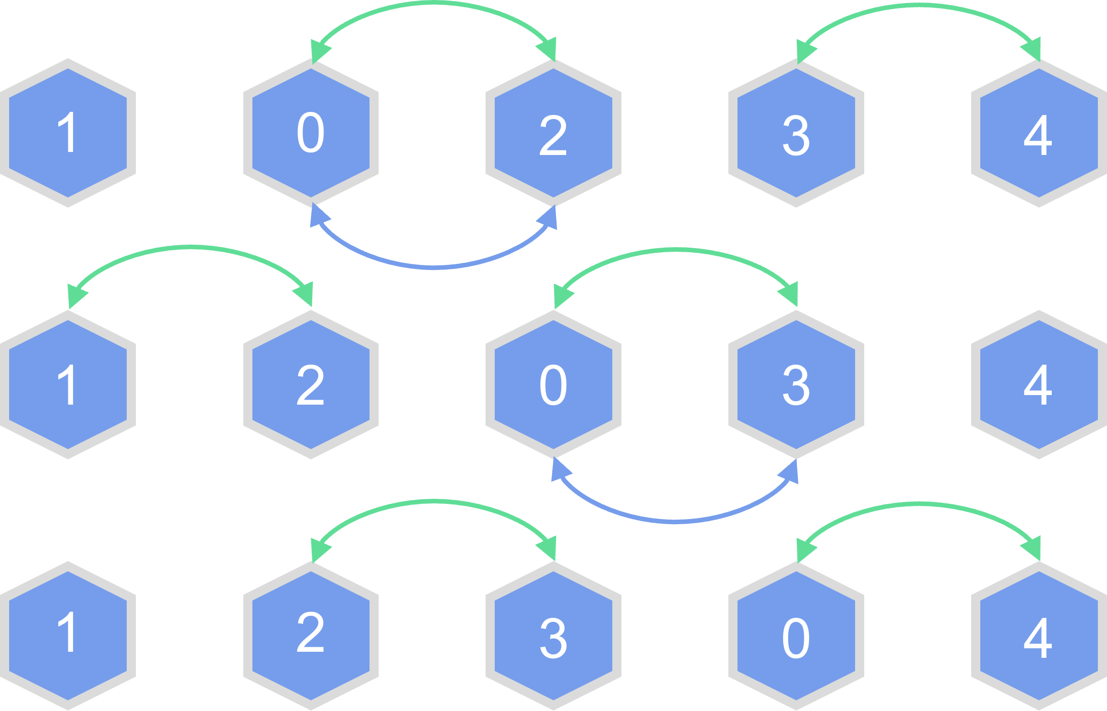

Different topologies will imply different counts of SWAPs added on top of the gates arising from the algorithm itself, as shown in Fig. 3. On a NISQ device, this implies different computational precision for the same gate error magnitudes. We choose the SWAP count as our metric to compare different topologies, as commonly gates have fidelities limited by calibration. The errors could be due to crosstalk, leakage, or filtering causing disturbances to the control signals. Under this scenario we want to minimize the gate count. On the other hand, for a highly tuned up device whose gates are limited by qubit coherence times, it would be optimal to minimize the circuit depth instead of the TQG count.
Assuming the gate errors are independent, the total error will be bounded by:
| (13) |
where is the number of two-qubit gates, the number of single-qubit gates, and is the SQG error. Consequently, reducing the gate count, especially , has an exponential effect on the precision of the computations, underlining the effect of minimizing the SWAP gate overhead. As SWAP gates are not native to the hardware, but must be compiled out of three CZ gates, their effective error rate is also much higher than those of native gates.
III.4.1 Square grid
A common choice in superconducting quantum chips is the square grid of qubits. It has high connectivity and is suitable for performing the surface code error correction when scaled to large enough qubit counts with fast measurement and feedback Fowler et al. 2012. The qubit routing problem on a square grid can be tackled using various numerical approaches Hirata et al. 2009; Li et al. 2019; Saeedi et al. 2010; Zulehner et al. 2018. However, these methods are inefficient. In our case, a tailored SWAP routing method, shown in Fig. 3a, has been chosen and developed in Appendix F that can be shown to be well suited from two perspectives. First, a comparison against the cited numerical approaches (shown in Appendix F) reveals that our routing method is better in terms of number of gates. Second, it is completely deterministic and does not rely on expensive numerical optimization methods. It can also be shown not to be far from optimal: on a square grid each qubit has at most 4 nearest neighbors, implying that any SWAP operation provides at most 3 new neighbors. For an all-to-all (ATA) interacting Hamiltonian there are interactions, to leading order, for a simulation performed on qubits (corresponding to nuclei and one NV center). This implies a lower bound of at least SWAPs for any SWAP pattern on the square grid topology. Our SWAP pattern with SWAPs, discussed in Appendix F, is thus not far from optimal.
III.4.2 Star architecture
A star topology allows to implement the simulation of the simplified case without internuclear interactions directly, without any SWAP gates. With internuclear interactions considered, we still find a reduction in SWAP gates as compared to the square grid topology, as shown in Fig. 3b. This reduction comes from the SWAP routing we implement, that consists of making the qubit in Fig. 3b interact with all the external qubits and then swap its state with that of qubit and repeat this process until all interactions have been performed. This allows us to use only SWAP gates. The percentage of SWAP gates that can be saved can be observed in Fig. 4.
However, this improvement in the number of gates comes with a price to pay in the depth of the algorithm. We can only do one TQG at a time in the star chip and we have TQGs from simulating the physical interactions and TQGs from the SWAPs. This yields a depth for the TQGs of in a star chip, while for a square grid it is . Such depth increase comes from the reduction in parallelization, since all gates now act via the central qubit. On the other hand, less parallelization reduces the types of possible crosstalk errors. Adding connections between external qubits reduces the depth of the circuit, since the main cause of circuit depth is the fact that the interaction of two external qubits needs to be done exclusively by the central qubit. Further studies are required to see if the addition of more external layers to this topology (such as in a spiderweb) can lead to better compromises between depth and gate count, especially for simulating systems with clusters of strongly interacting nuclei.

III.5 Gate-level optimization
The two-qubit interactions that appear in the algorithm are the , and interactions, as shown in section III.3.2 and Fig. 2b. When compiling the algorithm into the native gates of the device, all these interactions must be implemented in terms of some available gate set. We study in Table 1 the overhead introduced by decomposing these interactions into different examples of native TQGs of superconducting devices; namely, the parametrizable and fixed-phase gate, the fixed-phase controlled- gate , and the gate. The gate is usually performed by making use of the cross-resonance gate Krantz et al. 2019; Magesan and Gambetta 2020, which introduces an interaction, making it equivalent to the for the purpose of this algorithm. We assume that the SQGs that can be implemented are the and the gates. These numbers can be further reduced if the first and last SQGs introduced by this compilation are combined with the adjacent SQGs in the algorithm.
| CNOT | ||||
|---|---|---|---|---|
| TQGs | ||||
| SQGs |
The conclusion is that fixed-angle gates will double the number of TQGs that need to be physically performed. In Ref. Lacroix et al. 2020, the improvements coming from the reduction of the gate count are compared to the new errors introduced by the interpolation of the calibrated phases. For two instances of a Quantum Approximate Optimization Algorithm (QAOA) Farhi et al. 2014, it is shown that the performance is better when using parametrized TQGs.
The gate sequences for some of the gate decompositions are shown in Fig. 5.
IV Co-Design hardware


(b) Electrical diagram of transmon qubit (left) coupled to a resonator mode (right) via a tunable coupler (center). The qubit has frequency , coupler , and resonator . The qubit and resonator have a direct capacitance and capacitances and respectively to the coupler.
A star-architecture chip has fundamental scaling issues using a transmon as the central qubit as the number of neighbors grows. Every neighbor added to the center qubit would decrease its charging energy . To keep the qubit frequency constant and anharmonicity in the transmon regime, the ratio of the qubit’s Josephson energy to its charging energy, , must remain unaffected. Therefore we cannot afford to change its charging energy. This leads to a trade-off between the number of coupled qubits and their coupling strength to the central element.
The spirit of Co-Design calls for replacing the central transmon with another object that enables this scaling in size. A resonator has no Josephson energy , so the ratio is not altered by adding more capacitive couplings to the resonator. Only small corrections to its frequency are introduced by adding coupled qubits. As a distributed element, a co-planar waveguide resonator also has physically more space for couplings than a central transmon qubit. By elongating the resonator and choosing the mode with the target frequency, the number of qubits coupled to it can further be increased. These properties make a resonator a favourable component in the center of the chip.
In the device in Fig. 6a the qubits are capacitively coupled to the resonator via tunable couplers Mariantoni et al. 2008; Yan et al. 2018; Foxen et al. 2020 in the proximity of a voltage maximum of a standing wave in the resonator. As the resonator is elongated, we must use higher harmonic excitations of the resonator to keep the frequency around the operational frequency of the qubits. Tunable couplers avoid the frequency crowding issues related to direct coupling Song et al. 2017; Song et al. 2019, and the linear resonator has higher connectivity in the center than ring resonator structures with quasi-all-to-all connectivities Hazra et al. 2021.
A linear resonator cannot in general be used as a qubit, since a microwave drive on it will not only populate the subspace, but also higher excited states. However, the effective interactions mediated via the tuneable coupler in Fig. 6a are of the type and where and Krantz et al. 2019 are the resonator creation and annihilation operators. These types of interactions conserve excitation number, so when at most one excitation is in the qubit-resonator system, the resonator cannot be populated beyond its first excited state through interaction with a qubit mediated a tuneable coupler.
CZ and iSWAP gates between the resonator and a qubit can be performed using the two interactions, and the theory is developed more fully in Sec. IV.1. Then, a resonator together with an external qubit can be used as an effective central qubit in the following way:
- 1.
Prepare all qubits and the resonator in their ground states
- 2.
Select one qubit to form the effective central qubit together with the resonator
- 3.
Prepare an arbitrary state in the selected qubit
- 4.
Perform an iSWAP operation from the selected qubit to the resonator initially in the ground state
- 5.
Perform CZ gates between the resonator and any other qubits
- 6.
Perform an iSWAP operation back from the resonator to the selected qubit for measurement
The theoretically most straightforward protocol would be to perform a SWAP gate from the qubit to the resonator. The iSWAP, on the other hand, is a native gate that can directly be implemented on the hardware in Fig. 6b. The iSWAP gate between the resonator and the qubit is represented by the unitary operator:
Since the CZ gates performing the computation following the iSWAP are diagonal in the computational basis, the phase introduced by the iSWAP is uninvolved in the gate. This enables substituting the SWAP gate by an iSWAP gate in the protocol to further minimize the gate count.
IV.1 Gate theory and simulations
Here we demonstrate that in our star architecture CZ and iSWAP-type gates between any of the qubits and the subspace of a chosen resonator mode can be implemented. The operational principles of these gates are very similar to those between two qubits coupled with a tunable coupler Mariantoni et al. 2008; Yan et al. 2018; Foxen et al. 2020; Chu and Yan 2021. The main limitation of our architecture (where one transmon is replaced by a resonator) is that iSWAP operations can only be performed in the zero- and single-excitation subspace of the two-qubit computational basis.
| Parameter | Symbol | Value |
|---|---|---|
| Resonator frequency | 24.3 GHz | |
| Qubit anharmonicity | - 20.187 GHz | |
| Coupler anharmonicity | - 20.110 GHz | |
| Resonator-coupler coupling | 298.5 MHz | |
| Qubit-coupler coupling | 2101.8 MHz | |
| Resonator-qubit coupling | 28.9 MHz | |
| Resonator relaxation | 60 | |
| Qubit relaxation | 60 | |
| Coupler relaxation | 30 | |
| Resonator dephasing | 60 | |
| Qubit dephasing | 60 | |
| Coupler dephasing | 30 |
IV.1.1 Conditional-Z gate
The CZ operation between the resonator and the qubit is described by the unitary operator:
This gate is equivalent to the gate in Eq. III.2.1 up to two -rotations. To operate a CZ gate, we initialize the resonator-coupler-qubit set up shown in Fig. 6b at the idling configuration with zero effecting coupling between the qubit and resonator. Note that the coupler is also a transmon that shows a higher sensitivity to the magnetic flux than regular qubits. We next apply a flux pulse that lowers the coupler frequency, turning on the effective coupling between the resonator and the qubit. Depending on the flux pulse shape, the state collects conditional phase and possibly experiences population oscillations between computational and non-computational states, as a function of the time spent at the gate-operation frequency. We optimize the pulse amplitude and duration such that after the flux pulse the CZ gate fidelity is maximized. Details of the gate theory can be found in Appendix G and the considered device parameters in Table 2.
In Fig. 7a, we operate our CZ gate by tuning the coupler frequency using a flattop Gaussian shaped flux pulse. The width of our Gaussian filter was fixed at 3 ns. Applying such a flux pulse to coupler results in a coupler frequency shift by from the idling configuration. Then by appropriately tuning and the gate time , one locates the optimal pulse configuration that minimizes the CZ() gate error , where is the target density matrix obtained after propagating some initial state with the ideal unitary of Eq. IV.1.1 and the final density matrix obtained after propagating with the Lindbladian corresponding to our system defined in Eq. (60). For our device parameters, the maximal decoherence limited CZ gate error averaged over a number of random initial states is . Note that the system parameters in Table 2 were chosen such that they allow for the possibility to find a good idling configuration, where the residual CZ interaction vanishes before the gate operation. In our simulations, we have included environmental noise, such as amplitude damping and pure dephasing and treated them using a Lindblad master equation solver in QuTiP Johansson et al. 2012; Johansson et al. 2013.


IV.1.2 iSWAP gate
Just as the CZ gate, the iSWAP gate can be natively realized in superconducting quantum computing architecture Krantz et al. 2019. With our device, we can perform high-fidelity iSWAP gates between zero- and single-excitation computational states. The two-photon state , where denotes the first excited state of the resonator, must be excluded because it resonantly interacts with the state inducing a population exchange between the states. Hence the resulting operation in this subspace does not match the action of the targeted iSWAP operation.
The capacitive coupling between the elements of the electrical circuit shown in Fig. 6b gives rise to an effective -interaction between the qubit and resonator under the rotating wave approximation. Such an interaction conserves excitation number. With only the qubit or resonator (or neither) initially populated, we stay within the single excitation subspace of the joint system, thereby minimizing leakage of quantum population into the higher excited states of the resonator. The -interaction can be turned on by first tuning the qubit in resonance with the resonator, and then applying a flux-pulse to the coupler to turn on the coupling, similar to the CZ gate operation.
Fig. 7b shows iSWAP gate error landscape for the same device parameters (given in Table 2). The optimal average iSWAP gate error obtained for our device is . This result is obtained by averaging over a number of random initial states within the zero- and one-excitation manifolds.
The results of our two-qubit-gate simulations demonstrate that our star architecture supports operating gates with similar fidelities as regular transmon qubits coupled together. The increased local connectivity of the device reduces the need for SWAP gates to simulate the nanoscale NMR problem (and others with a similar structure) and consequently in the end improves simulation fidelities.
IV.2 Reset
The hyperpolarization protocol described in Sec. II needs regular re-initializations of the state of the NV center. The Co-Design hardware for simulating the protocol must therefore support this operation within qubit lifetimes. This is a hardware challenge, but one with solutions in sight. In particular, the quantum circuit refrigerator (QCR) has been used to perform the reset in tens of nanoseconds Tan et al. 2017; Silveri et al. 2017; Hsu et al. 2020; Sevriuk et al. 2019, which is a similar timescale to gate operations. The advantage of using a QCR for the reset is the possibility to reset the central resonator directly, without the need transfer the resonator population back to the central qubit using an iSWAP gate. Alternatively, a fast reset is possible through applying a flux drive to a qubit to SWAP its state with its measurement line Zhou et al. 2021. This scheme has the advantage of not requiring any additional hardware not already present on the chip, but comes with a small cost in the circuit depth, as the state of the resonator must be transported using an iSWAP gate into the designated central qubit and be re-initialized there. The reset timescale is also somewhat longer than when using a QCR.
V Results and discussion
In this section we discuss the two main results of the paper: namely the predicted performance of our proposed quantum algorithm on a regular noisy QPU, as well as the performance increase obtained with our proposed Co-Design QPU. To this aim, we will focus on the polarizations of the NV center and nuclear spins, that are relevant quantities of the problem and straightforward to measure in a quantum computer.
In Fig. 8 we compare the frequency response of the polarization transfer process on two different simulated devices: a QPU with realistic noise parameters, and an ideal noiseless QPU. We consider one NV center, two interacting nuclei and different driving frequencies for both continuous and pulsed driving schemes. In the simulation we ignore errors in the preparation of the fully-mixed state of the qubits representing the nuclei. The blue curves show the remaining polarization in the NV center after one cycle of initialization and time evolution, while the red and the green curves correspond to the nuclear polarizations at the end of the cycle. For each nucleus there appears a resonance frequency in the system, for which the polarization transfer is optimal for said nucleus, depicted in the figure by the peaks of the curves.
Both simulations include the effects of the most common imperfections in nanoscale NMR systems, i.e. energy detunings and Rabi frequency fluctuations discussed in Sec. II. The simulation of the quantum algorithm additionally includes noise and gate errors present in the QPU. It is notable that the noise affects the height and shape of the peaks more than their location.
The system imperfections include a detuning of kHz of the NV center from the zero-field splitting that shifts the peaks in Fig. 8 (left) to frequencies lower than their predicted Larmor frequencies (dotted vertical black lines). Fig. 8 (right) shows how the pulsed-driving scheme XY8 Maudsley 1986; Gullion et al. 1990 acts as a robust dynamical decoupling sequence, eliminating such frequency shifts both in the ideal and noisy simulations.
Regarding the QPU noise and errors, the amplitude damping channel causes an overall shift down of all polarizations at all driving frequencies. Dephasing noise and gate errors (as modelled by depolarizing noise) cause the curves in Fig. 8 to flatten and lose contrast. While we have discussed how the product of gate errors is minimized by reducing the SWAP overhead through Co-Design hardware, the loss of contrast can also be addressed through error mitigation techniques such as zero-noise extrapolation Endo et al. 2018; Cai 2021; Krebsbach et al. 2022. Dephasing can also be reduced through dynamical decoupling techniques Krantz et al. 2019, thus extending the system coherence and increasing the effective time. The simulations presented in Fig. 8 include the decoherence times and gate fidelities that can be achieved with the hardware in Sec. IV. This implies an overestimation of the actual errors in the simulation, since the gate fidelities already include some decoherence.
To quantify the advantage of our Co-Design processor, Fig. 9 shows how the reduction in TQGs improves our ability to extract relevant information from the simulation. The figure compares the star-architecture chip to qubits connected on a square grid simulating a six qubit system with one NV center and five non-interacting nuclei. On the two chips we use SWAP patterns according to the schemes discussed in Sec. III.4.
First, Fig. 9a shows the average height-to-width ratio of the nuclear polarization peaks obtained with star and square grid topologies with respect to an ideal error-free simulation. It serves as an indicator of how much the QPU noise degrades the simulation for each case. The ratio is computed by fitting a Gaussian function on each peak, and computing:
| (22) |
where is the height and the variance of the fitted Gaussian function, averaged over the five nuclei.
The curves for both topologies must coincide at for a maximal-error device, and at for an error-free quantum computer, since for a maximal-error device the output is pure noise and for an error-free quantum computer the number of SWAPs is irrelevant to the precision. For NISQ devices in between these limits, a performance difference between the architectures is observed. For systems with more nuclei and NV centers, the differences between topologies start to appear at lower errors, since the number of total operations grows. This shows how the QPU topology is of great importance for the computational precision of NISQ devices, while for fault-tolerant quantum computers the precision is unaffected by the topology.
Second, Fig. 9b shows the average relative error in the central frequency of the NMR peaks:
| (23) |
where and are the peak-center frequencies extracted from the Gaussian fittings for the noisy and ideal cases, respectively. The peak centers correspond to driving frequencies that efficiently transfer polarization to different parts of the diamond lattice.
With the quantum simulation we can individually identify the nuclear resonance peaks by directly measuring the polarization of each qubit. This could enable exploration of how the polarization diffuses in the lattice with single-nucleus precision. In contrast, in a standard nanoscale NMR experiment, one typically only has only access to the excitation loss of the NV ( and thus only to the average transmitted polarization). This demonstrates the advantage of simulating the system on a quantum computer, as a it provides access to the relevant microscopic details of the dynamics that are otherwise inaccessible.
The figures demonstrate that the Co-Design chip is able to detect the resonance frequencies and predict the peak heights better at all considered noise levels. The power of Co-Design is particularly evident in Fig. 9b, where the square grid is shown to require two orders of magnitude lower noise levels to reach the same accuracy as the Co-Design chip.
VI Conclusions and outlook
We have presented a quantum algorithm to simulate a nanoscale NMR problem, namely a hyperpolarization protocol. We have simulated the proposed quantum algorithm with typical noise processes of a NISQ superconducting quantum computer with state-of-the-art parameters. We find that, despite considering a noisy QPU, our protocol still allows to identify the positions of the nuclear resonances (corresponding to the maximal polarizations) in the frequency domain, as well as the behavior in the vicinity of such resonant frequencies, thus enabling the exploration of optimized protocols and driving parameters to hyperpolarize the nuclear ensemble.
Moreover, we have shown that a specific Co-Design architecture adapted to the problem provides an advantage over general-purpose designs in the NISQ era, thanks to the reduction in two-qubit-gate count. Consequently, the adapted design reduces the necessary gate fidelities to solve practical problems in nanoscale NMR. This application-specific QPU consists of a central resonator, representing an NV center, coupled to a number of qubits representing the nuclei. The design can be scaled to more NV centers and a potentially large number of qubits around them. This is an example of a shortcut to quantum advantage. Adapting more NISQ-friendly algorithm alternatives, such as those listed in Bharti et al. 2021, adapted to the problem and to the Co-Design hardware can provide further shortcuts.
Our work opens interesting directions for further investigation, since a quantum processor able to efficiently simulate nanoscale-NMR scenarios with a large number of nuclear spins would have a great impact on NMR-based applications. Fast and reliable quantum simulations of interacting spin systems would improve the interpretability of zero- and low-field NMR where spin-spin interactions become dominant Seetharam et al. 2021, and nanoscale-NMR systems where a quantum sensor is strongly coupled via dipole-dipole interactions to nuclear or electron spin clusters. A possible application of the latter is the estimation of inter-label distances (via, e.g., Bayesian analysis of the NV center response) in electronically labelled biomolecules Munuera-Javaloy et al. 2021b. In this case, the numerical analysis of systems beyond two-electron spin labels in realistic conditions, including protein motion and decoherence channels, is already numerically challenging.
Acknowledgments
The authors would like to thank Caspar Ockeloen-Korppi, Alessandro Landra and Johannes Heinsoo for their help in developing the idea of the star-architecture chip, Jani Tuorila for his support in developing the gate theory, Amin Hosseinkhani and Tianhan Liu for reviewing the manuscript, and Henrikki Mäkynen and Hoang-Mai Nguyen for graphic design. J.C. additionally acknowledges the Ramón y Cajal program (RYC2018-025197-I). We further acknowledge support from Atos with the Quantum Learning Machine (QLM). Finally, the authors acknowledge financial support to BMBF through the Q-Exa project No. FZK: 13N16062.
Appendix A Derivation of the system Hamiltonian
The Hamiltonian in Eq. (1) can be derived from first principles. Let us first assume a model including only two nuclei and one NV center (Fig. 1) with dipole-dipole interactions. For simplicity we also consider the NVs to be aligned with the external magnetic field. In that case, the Hamiltonian of the system reads:
| (24) |
where is the -th spin component of the NV center, the -th spin component of nucleus , is the zero-field splitting of the NV center, and are the gyromagnetic factors of the NV center and the nuclei respectively, is the external magnetic field, which is aligned with the symmetry axis of the NV center is the relative position vector between the NV center and nucleus and is the relative position vector between both nuclei.
We go into an interaction picture with respect to . The -nuclei interaction term reads:
| (25) |
where we split the expression in commuting and non-commuting operators. The non-commuting operators pick a fast-rotating phase and can be neglected through the rotating-wave approximation. By performing an interaction-picture transformation with respect to , the nucleus-nucleus interaction term reads:
| (26) | ||||
with . Applying again the rotating-wave approximation and undoing the interaction picture we finally arrive at:
| (27) |
with , and .
We rewrite in the subspace by dropping out the energy state as it will not participate in the dynamics. Leakage to that state would not be a problem because of the energy difference between states and . Then by using that to we get:
| (28) |
where is the modified nuclear Larmor term due to the presence of the NV center.
Appendix B Hyperpolarization sequences
B.1 Hartmann-Hahn sequence
Here we explain the dynamics induced by the continuous driving on the hyperpolarization protocol. To illustrate the mechanism, we consider a system including a single NV center and a single nucleus. The corresponding Hamiltonian, now including the driving term, reads:
| (29) |
In the interaction picture with respect to we obtain:
| (30) |
where . Choosing the resonance condition and applying the rotating-wave approximation we get:
| (31) |
Finally we can use the identity and the fact that there will be no transitions to the because of energy differences:
| (32) |
where and . More details about the different terms were discussed in the main text, in section II. Choosing and further moving to an interaction picture with respect to the terms we obtain:
| (33) |
We choose now , leading to the so-called Hartmann-Hahn double-resonance condition. Applying the identity and the rotating-wave approximation to remove time-dependent terms, we get the flip-flop Hamiltonian:
| (34) |
with and the nuclear coordinates changed so that and with .
B.2 Pulsed sequence
Now we consider the pulsed case, represented by the driving term where is a train of -pulses. The Hamiltonian is already expressed in the interaction picture from Eq. (32). From there, we further move into a rotating frame with respect to the driving term. The corresponding unitary transformation is for the time interval between pulses and . This leads to:
| (35) |
where is the so-called filter function, with value when is even, and when is odd, representing the sign of the operator , flipped by the action of each pulse.
It is necessary to apply two different patterns of pulses. The ”symmetric case”, meaning an evenly-distributed sequence of pulses for which the filter function is even and can be expanded in Fourier series of cosines as:
| (36) |
with when is even and when is odd, if the pulses are distributed such that the interpulse spacing is constant. We choose the resonance condition , where is the harmonic number. This is the same resonance condition that we introduced in section II, but here it is formulated with the period that appears in the Fourier expansion, instead of with the interpulse spacing from before. Going to an interaction picture with respect to and repeating the procedure we used above in the Hartmann-Hahn case, we get:
| (37) |
where .
With the second pattern of pulses, called the ”asymmetric case”, we apply an oddly-distributed sequence of pulses for which the filter function is odd and can be expanded in a Fourier series of sines. Note that this sequence of pulses is identical to the even sequence but shifted by a phase. An analogous derivation gives:
| (38) |
with and coming from the Fourier expansion of sines, analogously to .
Combining these two patterns one can generate an effective Hamiltonian of the form:
| (39) |
which can be transformed with simple rotations on the qubit representing the NV into:
| (40) |
and this is equivalent to an interaction-exchange flip-flop Hamiltonian, similar to the one for the continuous-driving case (34). A more detailed description of this whole process, including the expressions of the Fourier coefficients and can be found in reference Munuera-Javaloy et al. 2021a.
In order to visualize the structure of the pulsed-driving case, we have included in Fig. 10 the circuit implementing all these terms on a quantum chip for the case of one NV center and two nuclei.

Appendix C Randomized Trotter techniques
As explained in section III, we chose Trotter expansion. Besides this, we can consider other simulation approaches such as the variational quantum simulator Yuan et al. 2019, the quantum assisted simulator Bharti and Haug 2021, numerical quantum circuit synthesis Younis et al. 2021, or a plethora of other quantum simulation algorithms aimed at NISQ devices Bharti et al. 2021.
In addition, other approaches like randomized Trotter have been recently shown to provide some advantage compared to standard Trotter expansions Childs et al. 2019. We also propose to use one randomized approach, qDRIFT Campbell 2019, that consists of the following: instead of splitting the whole evolution operator into simpler terms as done in full Trotterization, the method applies a random selection of such terms to the quantum circuit. This random selection is based on the probability distribution given by the weight of each term . For a certain evolution time, this set of gates can approximate the whole evolution operator by statistically drifting the state of the circuit towards the deterministic final state.
The error bound for this method is given as Campbell 2019:
| (41) |
where and is the number of individual two-qubit evolution operators that are implemented. These evolution operators have the form , being a constant related to the relative weight that the term has in the Hamiltonian.
The advantage of qDRIFT compared to Trotterization is particularly apparent when dealing with Hamiltonians with a large number of terms with small coefficients, simulated for short times. While in the standard Trotter case, every term has to be simulated for each step no matter how small its effect is, in qDRIFT this is not required. A more thorough analysis of errors in qDRIFT and gate counts can be found in Chen et al. 2021.
This method is particularly suitable to our problem, since the range of coefficients in the Hamiltonian of a real diamond is large due to the length scales involved.
In this case, with qDRIFT the terms with smaller coefficients do not add a significant amount of gates as they would in conventional Trotterization approaches.
We note that other adapted protocols such as SparSto Ouyang et al. 2020 can further enhance the simulation of this type of systems. SparSto represents a compromise between Trotterization and qDRIFT, generally guaranteeing an equal or better performance than both of them. We will not go into detail on this method since Trotterization and qDRIFT are enough to illustrate the main ideas behind this work.
Appendix D Hamiltonian decomposition for Trotterized time evolution
In order to simulate the dynamics generated by the Hamiltonian in Eq. (1) on a quantum computer using Trotterization, we first need to express it in a suitable way. To begin with, we split the Hamiltonian into two parts:
| (42) |
which can be expressed in terms of qubit Pauli operators:
| (43) |
| (44) | ||||
Since in the rotating frame with the drive the Hamiltonian is time independent, the time-evolution operator is simply given by:
| (45) |
where is the time for which the simulation runs.
The time-evolution operator is split into discrete steps through Trotter decomposition:
| (46) |
The evolution operator associated with single-qubit gates in each Trotter step of equation (46) needs to be rewritten in terms of our native gate set. It is always possible to decompose any single-qubit unitary exactly, up to a global phase, into a sequence of three single-qubit rotations such as, for example, a rotation about the -axis in between two rotations about the -axis:
| (47) |
where the angles and need to be determined from the specific entries of the unitary in question to simulate the evolution of the qubit:
| (48) |
From now on, we will concentrate on the case of a single NV center, which will be encoded in qubit . Then, the evolution operator associated to single-qubit gates for the NV center will be:
| (49) |
Matching the entries of the matrices corresponding to the unitaries on equations (48) and (49) we get a system of equations for the angles and for each Trotter step .
There are 3 (5) types of interaction terms of the form in without (with) internuclear interactions. Due to the native TQG being of only interaction type (see Eq. (III.2.1)), local rotations need to be introduced for simulating the rest of the TQG terms. These are , which have the effect of converting the Pauli operator into the Pauli operator for qubit .
After the Trotterization introduced in equation (46), the term corresponding to TQG contains some elements which do not commute with each other, and some of them which do commute with each other. We choose to split all terms in order to express the time-evolution operator in terms of the native gates that we assumed in section III.2.1. Only the elements that do not commute with each other contribute to the total Trotter error, which remains of the same order:
| (50) | ||||
Finally, we observe that the operators (and the rest of the TQG terms) commute with each other, so the exponentials can be further split without Trotterizing:
| (51) |
The time-evolution operator implementing the continuous sinusoidal driving is:
| (52) |
The quantum algorithm for simulating the system under a pulsed-driving scheme is somewhat more involved than the continuous-driving case, due to the two different time-dependent processes involved in the Trotter decomposition: the free dynamics of the spins and the sequence of pulses. The most crucial point to be aware of is the interplay between Trotter steps and interpulse spacing. The number of interpulse evolutions, i.e. number of pulses minus one, bounds from below the minimum number of Trotter steps for the simulation. Clearly, at least one Trotter step is needed for each interpulse evolution.
Taking this interplay into account, the most straightforward setup is to choose a frequency which will determine the spacing of the pulse sequence, and to identify each interpulse evolution with a single Trotter step. If the achieved precision is not high enough, more Trotter steps can be added for each interpulse evolution. Each -pulse itself is simply implemented as an - or -gate on the qubit representing the NV center. The OU-distributed Rabi frequency fluctuations present in nanoscale NMR systems are then simulated by over- and under-rotations of the - and -gates.
Appendix E Rotational optimization
In principle, we had a Hamiltonian with terms of the type , and for the case of no internuclear interactions. However, we can rotate the basis so the Hamiltonian loses the and terms, allowing to reduce the number of TQGs. To make up for this rotation, we need to introduce different constants for the problem and rotate the vector state we obtain at the end before measuring it. The rotations that we will consider are only one-qubit rotations on nuclei qubits and we are applying this just to the case with no internuclear interactions. Therefore, we can consider the effect of this rotation on only one qubit representing an arbitrary nucleus. We will exemplify this procedure using nucleus 1. If we want to obtain the mean value of acting on the nucleus:
| (53) |
where represents the evolution operator from to . The density matrix contains the state of the NV center (which is in the state at ) and nucleus 1, i.e. . Our intention is to obtain an expression of this mean value in terms of the rotated evolution operators and later, we will find the appropriate rotation to be perfomed. Then, taking into account that the trace is invariant under a rotation we get:
| (54) |
This can be expressed as:
| (55) |
The density matrix of the nucleus is the identity. Thus, any rotation on nuclei qubits leaves the density matrix unaffected, leading to:
| (56) |
Then we need to rotate the system previous to the measurement. By using the invariance of the trace under cyclic permutations we get:
| (57) |
which is equivalent to introducing a counter-rotation in the circuit before measurement.
Now let us focus on the specific rotation we have to implement. Since the constants multiplying the Pauli matrices in the Hamiltonian are and (for nucleus 1), we can rotate the basis to obtain a representation in which the vectors have only -component for and thus, and terms are removed. The vectors before and after the needed rotation can be seen in Fig. 11.
To compute the new vectors (and thus the new coefficients for the gates of our algorithm), we can use Rodrigues’ rotation formula to rotate a vector an angle around a unitary axis :
| (58) |
being in our case, and , with .
For implementing the counter-rotation of this in the quantum circuit, we use:
| (59) |
Appendix F SWAP routing
Our qubit routing method consists of mapping the square grid to a linear chain with qubits labeled from 0 to . Then, in the simplified case of no internuclear interactions, the optimal SWAP method for the one-to-all interaction case on a linear chain can be used. For a single NV center the protocol goes as follows:
- 1.
Initialize the state of the NV center in the second qubit;
- 2.
Perform interactions with the first and third qubits;
- 3.
SWAP the NV center qubit to the right;
- 4.
Perform interaction with right qubit;
- 5.
Repeat steps 3-4 until all interactions have been achieved.
The pattern is seen in Fig. 3a denoted by the intense blue arrows. With internuclear interactions we need to perform a swap pattern that enables all-to-all interactions. The so-called odd-even mapping in Fig 3a is an efficient one Cowtan et al. 2019 represented by green arrows in Fig. 3a. This consists of swapping first all the even qubits with their right neighbors and then swapping all the odd qubits with their right neighbors. This way, we will obtain all-to-all interactions with SWAP gates and a total TQG depth of . A summary of the TQG counts is shown in Table 3.
To motivate the creation of a chip with a star topology and the use of an alternative linearized SWAP routing for a square grid instead of standard numerical approaches, a comparison between all the cases is provided in Fig. 12. A reduction in the number of SWAPs can be noticed for both the linear chain approach and the star-topology chip against standard numerical approaches for a square grid.


| All-To-All | Star topology | Square grid | |
|---|---|---|---|
Appendix G Qubit-resonator gate theory
In the following discussion, we consider gate operation between the resonator and one of the qubits, and neglect any effects that arise from the interactions with spectator qubits and other resonator modes. The time dynamics in such a system are determined by the Hamiltonian:
| (60) | ||||
where the uncoupled part of the total Hamiltonian is:
| (61) | ||||
where and are the annihilation operator and fundamental frequency for the mode , respectively, and is the anharmonicity of the mode . The interaction component of the Hamiltonian is:
| (62) | ||||
where , and denote resonator-coupler, qubit-coupler and resonator-qubit coupling frequencies. With the Hamiltonian of Eq. (60), we are now in a position to perform simulations of two-qubit gates by propagating a suitably chosen initial state.
Before the gate operation, we choose the idling frequencies for the qubit, resonator, and the coupler such that the CZ coupling rate is minimized. This CZ coupling rate is defined as:
| (63) | ||||
where corresponds to the eigenenergy of Hamiltonian in Eq. (60) with excitations in resonator and excitations in qubit with coupler being in the ground state. The point of minimal is also known as the idling configuration, which we found to be at GHz for the parameters given in Table 2. The CZ gate is operated by sending a flux pulse that modifies the coupler frequency , which then in the coupled basis modifies the frequencies and . This makes non-zero, so the system collects a CZ phase.
References
- Feynman (2018) R. Feynman, Simulating physics with computers, in Feynman and computation (CRC Press, 2018) pp. 133–153.
- Lloyd (1996) S. Lloyd, Universal quantum simulators, Science , 1073 (1996).
- Preskill (2018) J. Preskill, Quantum computing in the NISQ era and beyond, Quantum 2, 79 (2018).
- Bharti et al. (2021) K. Bharti, A. Cervera-Lierta, T. Kyaw, T. Haug, S. Alperin-Lea, A. Anand, M. Degroote, H. Heimonen, J. Kottmann, T. Menke, et al., Noisy intermediate-scale quantum (NISQ) algorithms, arXiv preprint arXiv:2101.08448 (2021).
- Smith (1997) M. J. S. Smith, Application-specific integrated circuits, Vol. 7 (Addison-Wesley Reading, MA, 1997).
- Hsu and Tseng (2021) K.-C. Hsu and H.-W. Tseng, Accelerating applications using edge tensor processing units, in Proceedings of the International Conference for High Performance Computing, Networking, Storage and Analysis (ACM, 2021).
- Lu et al. (2020) T. Lu, T. Marin, Y. Zhuo, Y.-F. Chen, and C. Ma, Accelerating MRI reconstruction on TPUs, in 2020 IEEE High Performance Extreme Computing Conference (HPEC) (IEEE, 2020) pp. 1–9.
- Staudacher et al. (2013) T. Staudacher, F. Shi, S. Pezzagna, J. Meijer, J. Du, C. A. Meriles, F. Reinhard, and J. Wrachtrup, Nuclear Magnetic Resonance Spectroscopy on a (5-Nanometer)3 Sample Volume, Science 339, 561 (2013).
- Nielsen and Chuang (2000) M. Nielsen and I. Chuang, Quantum Computation and Quantum Information (Cambridge University Press, 2000).
- Hogben et al. (2011) H. Hogben, M. Krzystyniak, G. Charnock, P. Hore, and I. Kuprov, Spinach – a software library for simulation of spin dynamics in large spin systems, Journal of Magnetic Resonance 208, 179 (2011).
- Seetharam et al. (2021) K. Seetharam, D. Biswas, C. Noel, A. Risinger, D. Zhu, O. Katz, S. Chattopadhyay, M. Cetina, C. Monroe, E. Demler, et al., Digital quantum simulation of NMR experiments, arXiv preprint arXiv:2109.13298 (2021).
- O’Brien et al. (2021) T. E. O’Brien, L. B. Ioffe, Y. Su, D. Fushman, H. Neven, R. Babbush, and V. Smelyanskiy, Quantum computation of molecular structure using data from challenging-to-classically-simulate nuclear magnetic resonance experiments, arXiv:2109.02163 (2021).
- Sels et al. (2020) D. Sels, H. Dashti, S. Mora, O. Demler, and E. Demler, Quantum approximate Bayesian computation for NMR model inference, Nature machine intelligence 2, 396 (2020).
- Sels and Demler (2021) D. Sels and E. Demler, Quantum generative model for sampling many-body spectral functions, Physical Review B 103, 014301 (2021).
- Levitt (2013) M. H. Levitt, Spin dynamics: basics of nuclear magnetic resonance (John Wiley & Sons, 2013).
- Doherty et al. (2013) M. W. Doherty, N. B. Manson, P. Delaney, F. Jelezko, J. Wrachtrup, and L. C. L. Hollenberg, The nitrogen-vacancy colour centre in diamond, Physics Reports 528, 1 (2013).
- Abobeih et al. (2019) M. H. Abobeih, J. Randall, C. E. Bradley, H. P. Bartling, M. A. Bakker, M. J. Degen, M. Markham, D. J. Twitchen, and T. H. Taminiau, Atomic-scale imaging of a 27-nuclear-spin cluster using a quantum sensor, Nature 576, 411 (2019).
- Munuera-Javaloy et al. (2021a) C. Munuera-Javaloy, R. Puebla, and J. Casanova, Dynamical decoupling methods in nanoscale NMR, EPL (Europhysics Letters) 134, 30001 (2021a).
- Munuera-Javaloy et al. (2021b) C. Munuera-Javaloy, R. Puebla, B. D’Anjou, M. B. Plenio, and J. Casanova, Detection of molecular transitions with nitrogen-vacancy centers and electron-spin labels, arXiv preprint arXiv:2110.14255 (2021b).
- Ajoy et al. (2018) A. Ajoy, K. Liu, R. Nazaryan, X. Lv, P. Zangara, B. Safvati, G. Wang, D. Arnold, G. Li, A. Lin, et al., Orientation-independent room temperature optical 13c hyperpolarization in powdered diamond, Science advances 4, 5492 (2018).
- Hartmann and Hahn (1962) S. Hartmann and E. Hahn, Nuclear double resonance in the rotating frame, Physical Review 128, 2042 (1962).
- Carr and Purcell (1954) H. Carr and E. Purcell, Effects of diffusion on free precession in nuclear magnetic resonance experiments, Physical review 94, 630 (1954).
- Meiboom and Gill (1958) S. Meiboom and D. Gill, Modified spin-echo method for measuring nuclear relaxation times, Review of scientific instruments 29, 688 (1958).
- Maudsley (1986) A. Maudsley, Modified Carr-Purcell-Meiboom-Gill sequence for NMR Fourier imaging applications, Journal of Magnetic Resonance (1969) 69, 488 (1986).
- Gullion et al. (1990) T. Gullion, D. Baker, and M. Conradi, New, compensated Carr-Purcell sequences, Journal of Magnetic Resonance (1969) 89, 479 (1990).
- Casanova et al. (2016) J. Casanova, Z. Wang, and M. B. Plenio, Noise-resilient quantum computing with a nitrogen-vacancy center and nuclear spins, Phys. Rev. Lett. 117, 130502 (2016).
- Uhlenbeck and Ornstein (1930) G. Uhlenbeck and L. Ornstein, On the theory of the Brownian motion, Physical review 36, 823 (1930).
- Cai et al. (2012) J. Cai, B. Naydenov, R. Pfeiffer, L. McGuinness, K. Jahnke, F. Jelezko, M. Plenio, and A. Retzker, Robust dynamical decoupling with concatenated continuous driving, New Journal of Physics 14, 113023 (2012).
- Gillespie (1996) D. Gillespie, Exact numerical simulation of the Ornstein-Uhlenbeck process and its integral, Phys. Rev. E 54, 2084 (1996).
- Ajoy et al. (2019) A. Ajoy, B. Safvati, Nazaryan, R., and et al., Hyperpolarized relaxometry based nuclear T1 noise spectroscopy in diamond, Nature communications 10 (2019).
- Suzuki (1976) M. Suzuki, Generalized Trotter’s formula and systematic approximants of exponential operators and inner derivations with applications to many-body problems, Communications in Mathematical Physics 51, 183 (1976).
- Campbell (2019) E. Campbell, Random compiler for fast Hamiltonian simulation, Phys. Rev. Lett. 123, 070503 (2019).
- Yuan et al. (2019) X. Yuan, S. Endo, Q. Zhao, Y. Li, and S. Benjamin, Theory of variational quantum simulation, Quantum 3, 191 (2019).
- Bharti and Haug (2021) K. Bharti and T. Haug, Quantum-assisted simulator, Physical Review A 104, 042418 (2021).
- Younis et al. (2021) E. Younis, K. Sen, K. Yelick, and C. Iancu, Qfast: Conflating search and numerical optimization for scalable quantum circuit synthesis, arXiv preprint arXiv:2103.07093 (2021).
- Hatano and Suzuki (2005) N. Hatano and M. Suzuki, Finding Exponential Product Formulas of Higher Orders (Springer, Berlin, Heidelberg, 2005) pp. 37–68.
- Krantz et al. (2019) P. Krantz, M. Kjaergaard, F. Yan, T. P. Orlando, S. Gustavsson, and W. D. Oliver, A quantum engineer’s guide to superconducting qubits, Applied Physics Reviews 6, 021318 (2019).
- McKay et al. (2017) D. C. McKay, C. J. Wood, S. Sheldon, J. M. Chow, and J. M. Gambetta, Efficient Z gates for quantum computing, Phys. Rev. A 96, 022330 (2017).
- Yan et al. (2018) F. Yan, P. Krantz, Y. Sung, M. Kjaergaard, D. L. Campbell, T. P. Orlando, S. Gustavsson, and W. D. Oliver, Tunable coupling scheme for implementing high-fidelity two-qubit gates, Physical Review Applied 10, 054062 (2018).
- Tan et al. (2017) K. Y. Tan, M. Partanen, R. E. Lake, J. Govenius, S. Masuda, and M. Möttönen, Quantum-circuit refrigerator, Nature communications 8, 1 (2017).
- Silveri et al. (2017) M. Silveri, H. Grabert, S. Masuda, K. Y. Tan, and M. Möttönen, Theory of quantum-circuit refrigeration by photon-assisted electron tunneling, Physical Review B 96, 094524 (2017).
- Hsu et al. (2020) H. Hsu, M. Silveri, A. Gunyhó, J. Goetz, G. Catelani, and M. Möttönen, Tunable refrigerator for nonlinear quantum electric circuits, Physical Review B 101, 235422 (2020).
- Sevriuk et al. (2019) V. Sevriuk, K. Y. Tan, E. Hyyppä, M. Silveri, M. Partanen, M. Jenei, S. Masuda, J. Goetz, V. Vesterinen, L. Grönberg, et al., Fast control of dissipation in a superconducting resonator, Applied Physics Letters 115, 082601 (2019).
- Celio (1986) M. Celio, New method to calculate the muon polarization function, Physical review letters 56, 2720 (1986).
- McArdle (2021) S. McArdle, Learning from physics experiments with quantum computers: Applications in muon spectroscopy, PRX Quantum 2 (2021).
- Fowler et al. (2012) A. G. Fowler, M. Mariantoni, J. M. Martinis, and A. N. Cleland, Surface codes: Towards practical large-scale quantum computation, Phys. Rev. A 86, 032324 (2012).
- Hirata et al. (2009) Y. Hirata, M. Nakanishi, S. Yamashita, and Y. Nakashima, An efficient method to convert arbitrary quantum circuits to ones on a linear nearest neighbor architecture, in 2009 Third International Conference on Quantum, Nano and Micro Technologies (IEEE, 2009).
- Li et al. (2019) G. Li, Y. Ding, and Y. Xie, Tackling the qubit mapping problem for NISQ-era quantum devices, in Proceedings of the Twenty-Fourth International Conference on Architectural Support for Programming Languages and Operating Systems (ACM, 2019).
- Saeedi et al. (2010) M. Saeedi, R. Wille, and R. Drechsler, Synthesis of quantum circuits for linear nearest neighbor architectures, Quantum Information Processing 10, 355 (2010).
- Zulehner et al. (2018) A. Zulehner, A. Paler, and R. Wille, Efficient mapping of quantum circuits to the IBM QX architectures, in 2018 Design, Automation & Test in Europe Conference & Exhibition (DATE) (IEEE, 2018).
- Magesan and Gambetta (2020) E. Magesan and J. M. Gambetta, Effective Hamiltonian models of the cross-resonance gate, Physical Review A 101 (2020).
- Lacroix et al. (2020) N. Lacroix, C. Hellings, C. K. Andersen, A. D. Paolo, A. Remm, S. Lazar, S. Krinner, G. J. Norris, M. Gabureac, J. Heinsoo, A. Blais, C. Eichler, and A. Wallraff, Improving the performance of deep quantum optimization algorithms with continuous gate sets, PRX Quantum 1, 110304 (2020).
- Farhi et al. (2014) E. Farhi, J. Goldstone, and S. Gutmann, A quantum approximate optimization algorithm, arXiv preprint arXiv:1411.4028 (2014).
- Mariantoni et al. (2008) M. Mariantoni, F. Deppe, A. Marx, R. Gross, F. K. Wilhelm, and E. Solano, Two-resonator circuit quantum electrodynamics: A superconducting quantum switch, Physical Review B 78, 104508 (2008).
- Foxen et al. (2020) B. Foxen, C. Neill, A. Dunsworth, P. Roushan, B. Chiaro, A. Megrant, J. Kelly, Z. Chen, K. Satzinger, R. Barends, et al., Demonstrating a continuous set of two-qubit gates for near-term quantum algorithms, Physical Review Letters 125, 120504 (2020).
- Song et al. (2017) C. Song, K. Xu, W. Liu, C. Yang, S. Zheng, H. Deng, Q. Xie, K. Huang, Q. Guo, L. Zhang, et al., 10-qubit entanglement and parallel logic operations with a superconducting circuit, Physical review letters 119, 180511 (2017).
- Song et al. (2019) C. Song, K. Xu, H. Li, Y. Zhang, X. Zhang, W. Liu, Q. Guo, Z. Wang, W. Ren, J. Hao, et al., Generation of multicomponent atomic Schrödinger cat states of up to 20 qubits, Science 365, 574 (2019).
- Hazra et al. (2021) S. Hazra, A. Bhattacharjee, M. Chand, K. Salunkhe, S. Gopalakrishnan, M. Patankar, and R. Vijay, Ring-resonator-based coupling architecture for enhanced connectivity in a superconducting multiqubit network, Physical Review Applied 16, 024018 (2021).
- Chu and Yan (2021) J. Chu and F. Yan, Coupler-assisted controlled-phase gate with enhanced adiabaticity, Physical Review Applied 16 (2021).
- Johansson et al. (2012) J. Johansson, P. Nation, and F. Nori, Qutip: An open-source Python framework for the dynamics of open quantum systems, Computer Physics Communications 183, 1760 (2012).
- Johansson et al. (2013) J. Johansson, P. Nation, and F. Nori, Qutip 2: A Python framework for the dynamics of open quantum systems, Computer Physics Communications 184, 1234 (2013).
- Zhou et al. (2021) Y. Zhou, Z. Zhang, Z. Yin, S. Huai, X. Gu, X. Xu, J. Allcock, F. Liu, G. Xi, Q. Yu, et al., Rapid and unconditional parametric reset protocol for tunable superconducting qubits, arXiv preprint arXiv:2103.11315 (2021).
- Endo et al. (2018) S. Endo, S. C. Benjamin, and Y. Li, Practical quantum error mitigation for near-future applications, Physical Review X 8, 031027 (2018).
- Cai (2021) Z. Cai, Multi-exponential error extrapolation and combining error mitigation techniques for NISQ applications, npj Quantum Information 7, 1 (2021).
- Krebsbach et al. (2022) M. Krebsbach, B. Trauzettel, and A. Calzona, Optimization of Richardson extrapolation for quantum error mitigation, arXiv:2201.08080 (2022).
- Childs et al. (2019) A. M. Childs, A. Ostrander, and Y. Su, Faster quantum simulation by randomization, Quantum 3, 182 (2019).
- Chen et al. (2021) C. Chen, H. Huang, R. Kueng, and J. A. Tropp, Concentration for random product formulas, PRX Quantum 2 (2021).
- Ouyang et al. (2020) Y. Ouyang, D. R. White, and E. T. Campbell, Compilation by stochastic Hamiltonian sparsification, Quantum 4, 235 (2020).
- Cowtan et al. (2019) A. Cowtan, S. Dilkes, R. Duncan, A. Krajenbrink, W. Simmons, and S. Sivarajah, On the Qubit Routing Problem, in 14th Conference on the Theory of Quantum Computation, Communication and Cryptography (TQC 2019), Leibniz International Proceedings in Informatics (LIPIcs), Vol. 135 (Schloss Dagstuhl–Leibniz-Zentrum fuer Informatik, Dagstuhl, Germany, 2019) pp. 5:1–5:32.