Fitting Sparse Markov Models to Categorical Time Series Using Convex ClusteringThanks: This material is based upon work supported by the National Science Foundation under Grant DM 1811933.
Abstract
Higher-order Markov chains are frequently used to model categorical time series. However, a major problem with fitting such models is the exponentially growing number of parameters in the model order. A popular approach to parsimonious modeling is to use a Variable Length Markov Chain (VLMC), which determines relevant contexts (recent pasts) of variable orders and forms a context tree. A more general parsimonious modeling approach is given by Sparse Markov Models (SMMs), where all possible histories of order are partitioned such that the transition probability vectors are identical for the histories belonging to any particular group. In this paper, we develop an elegant method of fitting SMMs based on convex clustering and regularization. The regularization parameter is selected using the BIC criterion. Theoretical results establish model selection consistency of our method for large sample size. Extensive simulation results under different set-ups are presented to study finite sample performance of the method. Real data analysis on modelling and classifying disease sub-types demonstrates the applicability of our method as well.
Keywords: Convex optimization, clustering, model selection, dimension reduction.
1 Introduction
Let be a categorical time series in discrete time, with finite state space . We suppose that the evolution of the time series follows an -th order Markov structure, where
| (1.1) |
for some . Here for any random vectors defined on a common probability space, we write to denote the probability distribution of given . Even when the alphabet is small, such as in applications involving binary chains or in genetics applications, complexity of the model (1.1) increases fairly quickly and parameter estimation may be difficult even for moderately large . Indeed, in the absence of a parametric model specification, the number of free parameters associated with (1.1) is given by which grows geometrically fast in the order , where denotes the size of the alphabet, that is the number of elements in .
Different dimension reduction strategies have been applied to reduce the model complexity in (1.1), such as Variable Length Markov Chains (VLMC) based on tree-structured conditioning sets. This idea was first introduced by Rissanen 1983, where relevant contexts (recent pasts) of variable orders are determined to form a context tree. In VLMC, , where , is the observed value of and the tree length may not be a fixed number, but rather is a function of the past values . In general, context tree models have parameters, where is the number of leaves in the context tree. That can take on arbitrary positive integer values for general context trees highlights the flexibility of a model with variable length contexts, and the fact that such models can lead to huge reductions in the number of parameters, especially when there is a long context in a single direction. A model of a variable order allows for a better trade-off between bias that arises through using contexts that are too short, and variance that increases with having many parameters, thus improving statistical inference. Bühlmann and Wyner 1999 and Bühlmann 2000 developed model selection strategies and studied asymptotic behaviour of Variable Length Markov Chains (VLMC). Recently, Kontoyiannis et al. 2020 and Papageorgiou and Kontoyiannis 2022 have developed inference and posterior representations for Bayesian Context Trees (BCT) for discrete time series analysis. These two papers also illustrate prediction in the BCT set-up using a posterior predictive distribution.
Roos and Yu 2009b and Roos and Yu 2009a pointed out that there can be relevant contexts that do not have the hierarchical structure of a context tree. Although they have discussed the possibility of more general models, the analyses of those papers were limited to the case where . Recently, researchers began studying sparse models posed in terms of a general partition of the set of all -tuples , where is the maximal order of Markovian dependence. Such models are called Sparse Markov Models (SMM), and introduce a sparse parametrization based on an unknown grouping of all possible th order histories . This generalization was first proposed by Garcıa and González-López 2011, who called it Minimal Markov Models. Later on, Jääskinen et al. 2014 developed Bayesian predictive methods to analyze sequence data using SMMs. Xiong et al. 2016 extended the previous paper, introducing a recursive algorithm for optimizing the partition for an SMM. Following a similar approach, Bennett et al. 2023 developed a method for fitting sparse Markov models using a collapsed Gibbs sampler. In this paper, we also consider SMMs in full generality, allowing an arbitrary and unknown number of groups. Specifically, let be a partition of . Then, the Markov chain in (1.1) is an SMM with groups if it satisfies the following sparse representation:
| (1.2) |
for each . Thus, for each , the transition probability remains unchanged over all -step histories lying in the set . This reduces the number of unknown probability parameters to . However, both the number of the sets in the partition and the sets themselves are unknown and must be estimated from the data.
To illustrate VLMC and SMM, we provide a very simple example of both models using DNA sequences with . In figure (1), we present the context tree of a VLMC of order with Level 0 representing the current time The tree structure indicates that for all histories of order with the most recent history being , the transition probability matrices are the same. A similar structure holds true for If the two recent histories are and then the transition probability matrices for all possible triplets are the same; and so on. Hence the given context tree corresponds to a partition of the 64 3-tuples of into 12 different groups, with contexts represented by the leaf nodes of the graph. However, for a SMM, the grouping can be arbitrary and does not necessarily have to follow a tree structure. One such example is portrayed in figure (2), where we enumerated the histories of a third-order Markov model as . These histories are partitioned arbitrarily into groups without any tree-like structure, where all histories in a given group have the same transition probabilities. Thus, VLMC form a special subclass of SMM.


The generalization to SMM introduces additional challenges for model fitting. Indeed, the task of identifying the true partition is a difficult problem even for moderately large . To appreciate why, note that the total number of partitions of , given by the well-known Bell number , grows at a very fast rate with the order (cf. De Bruijn 1981):
For example, with , , while . As a result, selecting the true partition from such a large collection of partitions is very difficult.
In this paper, we propose a novel approach for fitting Sparse Markov Models (SMMs) by leveraging recent advances in convex clustering. Our method addresses the challenges of determining the true model order and uncovering the latent partition structure in the space of observed -tuples. By treating the empirical transition probability vectors as data points, we apply convex clustering techniques—particularly the framework of Chi and Lange 2015—to group together those vectors that arise from the same underlying Markovian regime. The core idea is to minimize a penalized criterion function that encourages fusion of similar transition probabilities, leading to automatic partition recovery. The use of an appropriate convex distance metric ensures that the optimization remains tractable even for large values of , and enables scalable implementation. A data-driven BIC-based procedure is used to select the regularization parameter, and we establish theoretical guarantees for consistent model recovery. Through a comprehensive simulation study, we demonstrate the strong empirical performance of our method compared to existing approaches for SMM estimation. Finally, we apply our approach to a real-world classification task involving partial DNA sequences from respiratory viruses, achieving significantly lower mis-classification rates than alternative methods.
The rest of the paper is organised as follows. In section 2, we describe in detail the methodology for fitting SMM using convex clustering approach. Section 3 presents theoretical results, including model consistency guarantees. Section 4 reports simulation experiments comparing our method with existing techniques. Section 5 illustrates the application of our method to real virus classification data. Proofs of the theoretical results and some supplementary tables for simulation studies are given in the appendix.
2 Methodology
2.1 Notation
Let be the set of all positive integers, , and , for , . Write for an ordered (finite) sequence of -elements of length . Let denote the (ordered) concatenation of and . Write and w.l.o.g., set . Let so that . Let where denotes the indicator function. For any and , define and . In particular, denotes the number of times the chain hits the -tuple , and is the number of transitions from to . Note that denotes the total number of -th order histories in the observed variables .
Next we define the probabilities associated with the SMM (1.2). For and , let
and let be the corresponding transition probability vector. Note that by the SMM property, for any , the transition probability is a constant over all such that . However, we do not know the sets and determining them is one of the challenges of fitting an SMM to a data set. To that end, define non-parametric estimators of using their empirical versions:
and let be the transition probability vectors consisting of the elements .
Here we propose a new approach to fitting the SMM based on regularization.
2.2 Description of the Method
Consider the penalized criterion function
| (2.3) |
over for , where is a penalty parameter, are suitable nonnegative weights, is the -dimensional simplex and where is a distance measure between two -dimensional probability vectors. Thus, (2.3) treats the estimators as (correlated) “observations” and penalizes the distance between all distinct pairs of probability vectors in order to identify the identical probability vectors. In particular, the number of parameters grows at a rate proportional to the size of the true partition in the SMM and with a suitable choice of the penalization term, one can identify the identical probability vectors. When , (2.3) gives a version of the Group LASSO of Yuan and Lin 2006 that is designed for selecting pairs of full vectors that are close, and we have a convex optimization problem that can be solved for large On the other hand, if we use the distance , then only component-wise zero differences can be identified.
Once we minimize the criterion function in (2.3), it is a relatively easy task to find estimates of and the sets . Specifically, we start with a pair with the smallest and seek all such that the distance between the solutions and is zero. Then, we set to be the set consisting of and all such . In the next step, we consider all pairs that are not in and repeat the procedure until all pairs with estimated zero distances have been grouped. In case there are indices for which none of the estimated paired distances are zero, we keep them as singletons, that is groups consisting of single elements. This gives the estimated groups , with giving an estimate of .
In comparison, traditional clustering methodologies like -means have many limitations. In most cases, we have to pre-specify the number of clusters, along with the possibility that we end up with a local minima instead of the global one. The advantage of clustering by solving equation (2.3) for a range of is that we get a solution path from at most many singleton clusters to only one cluster consisting of all the elements. Subsequently, we can fix some criterion function which will enable us to find the optimum cluster assignment among all possible models in the solution path. Hence, not only do we not need to fix the number of clusters beforehand, but we also avoid the problem of being stuck at local minima. This particular approach will be broadly referred to as “Convex Clustering”.
2.3 Computational considerations
Several efficient algorithms have been developed in recent years to solve equation (2.3) when the penalty function is convex; e.g. for some . Pelckmans et al. 2005, Lindsten et al. 2011, Hocking et al. 2011 and others recently proposed this convex clustering approach and established it to be more robust and scalable in comparison to the traditional approaches. Lindsten et al. 2011 used an off-the-shelf convex solver CVX to solve the convex clustering problem, which suffers from scalability issues. Theoretical perfect cluster recovery conditions have been derived by Zhu et al. 2014 only for two clusters, while Panahi et al. 2017 derived perfect recovery conditions for general clusters, but under the assumption of uniform weights. Sun et al. 2021 provided sufficient conditions for theoretical recovery conditions under more general weight choices. They have also developed a faster algorithm called semismooth Newton based augmented Lagrangian method (SS-NAL), and derived the convergence criteria for their algorithm. Recently, Wang and Allen 2021 have introduced the Integrative Generalized Convex Clustering Optimization (iGecco) method for solving the convex clustering problem for more general loss functions, including non-differentiable ones. The major difference of our set-up from previous developments is that we cluster empirical transition probability vectors as opposed to the original data points.
While methods like iGecco (Wang and Allen 2021) have been developed for more general loss functions and are particularly useful in integrative clustering across multiple data modalities, our setup is more specialized. Specifically, we focus on clustering empirical transition probability vectors derived from categorical sequences using a squared error loss. The formulation of Chi and Lange 2015 aligns directly with this objective and provides efficient solvers tailored to squared loss with convex penalties. In contrast, iGecco’s flexibility for general loss functions introduces unnecessary complexity in our context. Therefore, we opt for the simpler and more specialized algorithm of Chi and Lange 2015, which has demonstrated strong performance under our model assumptions.
We now introduce the specific computational algorithm proposed by Chi and Lange 2015 that we use to minimize the objective function in (2.3). For , we first view solving equation (2.3) as the following constrained optimization problem
| (2.4) | ||||
where is the set of all distinct edges . Here, a new splitting variable has been introduced to capture the difference between the group centroids, which makes the optimization procedure much easier. Two algorithms have been developed for solving this constrained optimization problem, namely alternating direction method of multipliers (ADMM) and alternating minimization algorithm (AMA). ADMM solves constrained optimization problems by breaking them into smaller subproblems that are easier to solve, alternating between primal and dual updates. AMA simplifies the process further by avoiding auxiliary variable updates, leading to significantly faster convergence under sparse weights. For both of these algorithms, first we incorporate an augmented Lagrangian as follows:
| (2.5) | ||||
where and are the matrices with and for and in their columns respectively. Splitting the variables in such fashion would allow us to update , and sequentially, given the other variables. The convergence of ADMM does not depend on the choice of ; it is known to converge for any . On the other hand, AMA converges for any .
Since AMA provides much faster results, we will use this algorithm in numerical implementation of our methodology. Suppose, and be the parameter values in the step. The updates in the next step are computed using the following relations:
where , , and is the projection of onto the set . We continue until convergence, and the convergence criterion can be formulated using the dual problem and duality gap.
Initialize
2.4 Selection of the Tuning Parameter
So far, we have discussed the numerical methods to solve (2.3) for a given . But it is important to choose an optimum value of for the optimization problem. In this section, we propose a data driven method to select this tuning parameter using the BIC criterion. For a given , denote the obtained clusters as , where is the number of clusters. Define the common transition probability for the -tuples in the estimated group as
The log-likelihood of the observations under the obtained cluster assignment for a particular is given by
Hence, the BIC score corresponding to the obtained model is
By a grid search over a range of possible values, we select the for which BIC is minimized. The solution of equation (2.3) corresponding to that is considered as the estimated cluster assignment. The novelty of our method is that we are able to select the optimum tuning parameter from the data itself. For general convex clustering scenarios, one may not be able to compute the BIC criterion since the distributional properties of the data points in a cluster are unknown.
The assumption of Markovian structure is useful in our set-up to formulate the likelihood function. Moreover, the CLT-type results provide us the asymptotic distributions of the estimated transition probabilities. In the next section, we provide new theoretical results to demonstrate the model selection consistency under this BIC-based approach. We also provide some theoretical results and conditions under which the true partitions will appear in the solution path of convex clustering for a range of for large .
Alternative Selection via Pathwise Regularization.
In addition to the BIC-based grid search method, we also explored a pathwise convex clustering approach inspired by the algorithmic regularization framework of Weylandt et al. 2020. This technique efficiently constructs the solution path for varying values of without requiring full re-optimization at each point, by leveraging warm starts and algorithmic early stopping. Since this method produces the full solution path in the form of a dendrogram, we continue to use the BIC criterion to select the optimal model within this framework. In our experiments (see Section 4), the pathwise method yielded slightly lower clustering accuracy compared to the original BIC-guided convex clustering, but achieved substantial computational speed-ups. These properties make the pathwise strategy a promising alternative for high-dimensional categorical time series. While we primarily rely on the BIC criterion for theoretical tractability, the pathwise algorithm provides a scalable and empirically viable option.
3 Conditions and Theoretical Results
3.1 Conditions
We consider equation (2.3) with . Let the optimum solution be denoted by , for . Also, let the true partition of the state space be , with the corresponding transition probability vectors being . Thus, . Set , the size of the partition. Following the notation of Sun et al. 2021, define
We shall suppose
that the following conditions hold.
(A1)
and for any , .
(A2) , and .
In (A1) we assume symmetry, and that the weight is positive between two -tuples belonging to the same partition. (A2) gives a lower bound for the weight between two -tuple in a particular group.
Similar conditions have been used
by Sun et al. 2021 to prove
perfect recovery
results. In Theorem 3.6 below,
we provide some simple sufficient conditions on weight choices to satisfy these conditions.
Before going into the main results, we state two auxiliary results that will be used for the subsequent results.
Proposition 3.1.
Let be an aperiodic and irreducible SMM of order with true partition . Then, as ,
- (a)
for ;
- (b)
, where is the stationary probability of the state ;
- (c)
With ,
Since is of rank , the asymptotic Normal distribution is singular.
Thus, Proposition (3.1) asserts weak consistency and asymptotic normality of the estimated transition probability vectors, which can be proved using existing results on Markov chains in Billingsley 1961. The next result deals with perfect recovery under general weight choices under Conditions (A.1) and (A.2).
Proposition 3.2.
Suppose the above conditions (A1) and (A2) hold and . Then for any , for ; and for any . In other words, for any , we recover the true partition of the state space.
These propositions will be among the key tools used for proving our results. The CLT result will be useful for determining probability bounds for perfect recovery under the conditions of the proposition (3.2). In the next subsection, we state our major theoretical findings.
3.2 Main Results
Although the solution to the objective function in equation (2.4) involves optimization over vectors in , the feasible set is restricted to the probability simplex . As a result, the optimal solutions remain valid probability distributions over —that is, nonnegative vectors summing to one. We formalize this below and provide a short proof in the appendix.
Lemma 3.3.
For any , the optimal solution lies in the -dimensional probability simplex , i.e.,
- (a)
for all , and
- (b)
.
This result follows directly from standard properties of convex optimization over closed convex sets (see Boyd and Vandenberghe 2004) and the structure of the algorithm used (see Chi and Lange 2015). While one could impose simplex constraints explicitly during optimization, our augmented Lagrangian approach already preserves this structure without additional computational cost.
Despite this, we do not directly use the centroids from convex clustering as estimates of the transition probabilities. Due to the shrinkage effect induced by the fusion penalty, these cluster centers may be biased toward the global average and not accurately represent the true transition distributions. Therefore, once the partition is obtained, we re-estimate the transition probabilities for each cluster using the empirical frequencies of the histories in that cluster. This approach improves estimation accuracy while preserving the benefits of regularized clustering.
Next, we would like to derive the probability of true cluster recovery. There are two steps involved in this process. First, we need the true model in the solution path over varying . This implies the conditions of Proposition 3.2 must be satisfied, i.e. . From Theorem 3.4, which is given next, we get a lower bound on the probability of the true model being present in the solution path. Note that Sun et al. 2021 have derived these perfect recovery conditions for a given fixed data set when the data points in a particular cluster are close to each other. Our approach is significantly different, as we cluster estimated transition probability vectors, which are random variables, and thus and are random variables as well. We provide theoretical bounds to ensure that the probability of the event is .
Theorem 3.4.
Define
Then, under Conditions (A1) and (A2), as ,
for , and for some constants .
Looking at the expressions for and , it is evident that shrinks towards as increases as the estimated transition probability vectors and belonging to the same cluster become closer to each other. On the other hand, the different group means and tend to get separated from each other, making converge to a positive number, so that eventually we get . These expressions also tell us that in order to have perfect recovery of the clusters, a scaled version of the maximum within-group deviation of the transition probabilities should be less than a scaled version of the minimum between-group variation. These scales are heavily dependent on the choice of the weights . Note that, if we choose the weights in a way so that is higher if and are closer (and potentially belong to the same cluster), and lower if they are far from each other (potentially belonging to different clusters), the denominator of the term will be higher, and the denominator of will be lower in the ideal scenario. Hence, this particular choice of the weights will enhance separating and , increasing the chance of recovering the true cluster assignment. Although our theoretical guarantees are stated over a continuous subset of the real line for , in actual implementation we operate over a discrete grid of values. This is because the theoretical range depends on unknown model parameters and serves only as a sufficient condition for recovery.
Once we have the true model in the solution path, the next step is to establish that the probability of selecting that model through the BIC criterion converges to as . The next theorem gives a precise statement of this result.
Theorem 3.5.
Suppose the conditions of Theorem (3.4) hold, and . For any , denote the clustering assignment obtained by minimizing the equation (2.3) as ; where is the associated number of partitions of the -tuples. Suppose is the log-likelihood of the observations corresponding to cluster assignment , and the corresponding BIC score is . Choose some . Then, for any such that ,
as .
Theorem 3.5 asserts the consistency of the model selection using the BIC criterion and is one of the most important conclusions of this paper. Variable selection consistency results in Zhang et al. 2010 use a similar BIC-criterion for the LASSO penalty in multiple linear regression. However, our set-up is very different from the regression set-up (with independent observations). Further, the penalty function is quite different. As a result, the key steps for proving our result are very different. The consequence of this theoretical result is extremely important in applications. Even for moderately large sample sizes, we can achieve good clustering performance. We will demonstrate these properties for finite samples in the simulation study.
Although we have stated our results under conditions (A.1) and (A.2), we still need to check whether these conditions are feasible in practice. The next result provides sufficient conditions for perfect cluster recovery under a particular weight choice involving Gaussian kernels that also produces good clustering results in finite samples.
Theorem 3.6.
Define , and assume that the true cluster or partition sizes are different for the SMM. Suppose that
- (a)
, where is the indicator function that is one of the nearest neighbours of or vice versa, for some ;
- (b)
;
- (c)
for some , , , where
Then conditions (A1) and (A2) are satisfied. Moreover, and
Theorem 3.6 simplifies Conditions (A1) and (A2) for a special choice of weights, which we will use later in our simulation studies. The intuition behind this choice is that should be a decreasing function of which enforces less penalization for well-separated points. The following results are direct consequences of Theorem 3.6:
Corollary 3.6.1.
Under the assumptions of Theorem 3.4,
- (a)
, .
- (b)
.
Corollary 3.6.2.
For a balanced design, i.e. when are the same for all groups , if . Hence, for any , perfect recovery is possible for .
We present all proofs in the appendix section. Corollary 3.6.1 gives us an idea of how close the empirical transition probabilities for each -tuple are to the true probability vectors. Corollary 3.6.2 considers a special case when the design is balanced. In that scenario, for large and for the correct choice of the nearest neighbour, the true model can be retrieved for a wide range of tuning parameters , thereby providing very accurate clustering results. In the next section, we will explore the impact of weight choices on clustering accuracy through simulations of finite samples.
4 Simulation Study
In this section, we numerically evaluate the performance of the convex clustering methodology described earlier, focusing on its ability to recover the true cluster assignments. We compare clustering results across different choices of the weights , considering sparse Markov models (SMMs) of varying orders, sequence lengths, and alphabet sizes . Additionally, we benchmark our approach against several competing methods to demonstrate its practical utility. Specifically, we compare convex clustering with the BIC-based hierarchical clustering proposed by Garcıa and González-López 2011 (GGL), the Bayesian factor hierarchical clustering by Xiong et al. 2016 (Xiong), and the collapsed Gibbs sampler from Bennett et al. 2023 (GSDPMM), all of which are established techniques for estimating sparse Markov models or related structures. As a baseline, we also compare with -means clustering with several several values of , and then selecting the optimal model using BIC criterion. These comparisons provide insight into the relative accuracy and robustness of our method across a variety of scenarios.
Since our method does not require the number of clusters or their labels to be pre-specified, direct computation of the misclassification rate is not feasible. Instead, we use a standard metric to evaluate clustering accuracy: the Adjusted Rand Index (ARI) defined by Hubert and Arabie 1985, which measures the similarity between the estimated and true clusterings. A formal definition of ARI is provided in Appendix B.1.
We focus especially on how different weight choices influence ARI. Previous studies, such as Chi and Lange 2015 and Sun et al. 2021, have shown that using sparse weights improves both clustering accuracy and computational efficiency. We consider both dense and sparse weight matrices and assess their impact on clustering quality. We also use the pathwise approach of Weylandt et al. 2020 to dynamically trace the solution path and select the optimal based on BIC. Each simulation scenario is replicated 1,000 times to compute the mean ARI and standard error. We also report the empirical probability of perfect recovery—i.e., the proportion of replicates where ARI equals 1.
4.1 Simulation Set-up 1
We take , mimicking DNA sequence analysis. The order of the chain is . The possible histories are equally divided into groups of elements each. For each group , we generate independent , and then define group-wise transition probabilities via a Dirichlet distribution with parameter vector .
For convex clustering, we begin with uniform weights for all pairs. Next, we consider sparse weights based on estimated transition probability distances. Following Chi and Lange 2015, we use a -nearest neighbor (k-NN) approach with Gaussian kernel: , where indicates if is among the -nearest neighbors of or vice versa. We use and test and . We also explore two alternative weights: one using distance in the same form; another using Weylandt’s pathwise method to generate the full solution path and select the optimal model via BIC. We summarize the results in the following figure (3). We also present the results in details in the table (5) in the appendix.
From the figure (3), we observe that the uniform weights perform poorly in terms of ARI and perfect recovery, especially for smaller . In contrast, sparse weights with significantly outperform and the pathwise method at lower sample sizes. This aligns with Corollary 3.6.1, which supports as optimal in balanced settings. As expected, performance improves for all weight choices as increases.
Next, we compare our convex clustering method to the other competing methods and demonstrate the results in figure (4) and in the table (6). Convex clustering achieves higher ARI and recovery probability than all competitors, especially for small . Among competitors, GSDPMM is the closest in performance, followed by Xiong and GGL, both of which underperform. -means clustering performs the worst across all sample sizes, demonstrating the advantages of convex clustering for SMM estimation.
This setup achieves near-perfect recovery when . However, theoretical results suggest that well-separated centroids enable high recovery even for small . Here, with 4 groups (), the minimum centroid separation is in and in . The next simulation tests more well-separated settings.
4.2 Simulation Set-up 2
Here we take and . We divide this triplets into four groups of sizes and . For the group, , , , . We test three weight strategies:
- 1.
distance with Gaussian kernel and ,
- 2.
distance with exponential kernel and , i.e. ,
- 3.
distance with exponential kernel.
We also include Weylandt’s method, as well as all competitor methods used in Setup 1. Results for and are shown in the table (1).
| Method | CVX- | CVX- | CVX- | Weylandt | GSDPMM | Xiong | GGL | K-means | |
|---|---|---|---|---|---|---|---|---|---|
| 1000 | ARI | 0.816 | 0.908 | 0.893 | 0.904 | 0.916 | 0.637 | 0.265 | 0.883 |
| True Rec. | 0.000 | 0.104 | 0.030 | 0.108 | 0.104 | 0.000 | 0.000 | 0.104 | |
| 2000 | ARI | 0.954 | 0.983 | 0.979 | 0.983 | 0.984 | 0.786 | 0.634 | 0.948 |
| True Rec. | 0.140 | 0.638 | 0.468 | 0.660 | 0.683 | 0.013 | 0.000 | 0.538 |
From the experiment, we can infer that the convex clustering with weight involving distance in the Gaussian kernel performs poorly compared to or distance. Using distance is especially effective in such scenarios, as it measures the maximum element-wise distance between two estimated transition probability vectors. We are then able to separate out two vectors that are not likely to be in the same cluster. On the other hand, the competing methods like GSDPMM, k-means or Weylandt’s approach are also as good as convex clustering with distance kernel, sometimes providing a slightly better result for . Methods by Xiong et al. 2016 or Garcıa and González-López 2011 still perform worse than these methods for both sample size. This demonstrates that for well-separated clusters, we can actually use Weylandt’s approach to determine the optimal to get as good result as GSDPMM in much shorter time.
5 Real Data Analysis
In recent years, several viral outbreaks have posed serious public health challenges. Among them, the most widespread has been the COVID-19 pandemic, caused by SARS-CoV-2, which originated in Wuhan, China in late 2019 and spread rapidly across the globe. As of April 2022, there have been over 510 million confirmed cases and more than 6.2 million deaths worldwide. Symptoms commonly include fever, headache, fatigue, and respiratory distress, as reported by Wu and McGoogan 2020. Most cases are mild, with only 8–10% requiring hospitalization and a fatality rate of around 1.5%—lower than the 10% fatality observed during the 2002 SARS-CoV-1 outbreak and much lower than the 35% observed in the 2012 MERS-CoV outbreak in the Arabian Peninsula. Despite its lower mortality, SARS-CoV-2’s mild symptoms and high transmissibility have made it far more difficult to contain.
Diagnostic tools such as RT-PCR and rapid antigen tests have played a central role in pandemic response by identifying viral genetic material from saliva or mucus samples. While complete viral genomes can be matched to reference sequences for strain identification, in practice, clinical samples are often noisy, degraded, or partially observed—due to co-infections, sequencing limitations, or contamination. As a result, the problem of identifying the underlying virus from a partial genome becomes statistically challenging.
This difficulty is exacerbated when multiple viruses with similar symptoms co-circulate in the population. In the Indian subcontinent, for instance, Dengue virus is endemic during summer and fall, and shares many symptoms with COVID-19. Hepatitis B also presents with fever and fatigue, making clinical differentiation harder. In critical cases, incorrect identification may lead to inappropriate treatment or fatal outcomes.
In this work, we propose a sparse Markov model (SMM)-based classification framework to identify viruses from partially observed DNA sequences. The approach is designed to be statistically efficient, interpretable, and scalable, as demonstrated in our simulation studies. We now apply this methodology to a real dataset of 500 viral genomes spanning SARS-CoV-2, MERS-CoV, Dengue, and Hepatitis B, to assess performance under various levels of sequence truncation.
5.1 Data Description
We collected genome sequences for 500 individuals from the NCBI database, including 200 SARS-CoV-2, 50 MERS, 100 Dengue, and 150 Hepatitis B cases. The NCBI database also provides reference genome sequences, which represent canonical structures for each virus. These were used for model training. The lengths of the reference genomes are 29,903 (SARS-CoV-2), 30,119 (MERS), 10,735 (Dengue), and 3,542 (Hepatitis B).
MERS samples were collected from the 2012 outbreak in the Arabian Peninsula. Dengue and Hepatitis B samples span multiple countries and time periods over the last three decades. For SARS-CoV-2, we intentionally sampled 50 sequences from each of four critical time points: April 2020, September 2020, January 2021, and April 2021. These correspond to distinct waves or major strain transitions—such as the initial global spread, India’s first wave, the Beta wave in the U.S., and the emergence of the Delta variant in Asia. This strategy ensures temporal diversity and better representation of major SARS-CoV-2 variants.
5.2 Method
As mentioned earlier, our goal is to classify viruses based on partially retrieved genome sequences. To achieve this, we first model the four reference genome sequences using our proposed SMM approach with convex clustering. Next, we randomly select a continuous segment of the genome sequence for each sample, and then compute the likelihood of that segment under each of the reference models. Suppose the model is denoted by , . For any given sequence , likelihood of for each model is
We then classify to . Note that the transition probabilities inside the product term are estimated from the fitted model, along with . Thus, we expect that the true virus can be classified from a moderately large segment of the full RNA sequence of the respective viruses.
Apart from our proposed method using convex clustering, we also apply other SMM fitting methods in this setup. We apply GSDPMM, Xiong, GGL and K-means to estimate the partitions of the -tuples, and their corresponding transition probability vectors. Similarly, we compute the likelihood of a DNA sequence under each reference model, and classify the DNA sequence to the most likely virus.
Depending on the assumption on the order of the Markov chains, we fit two different models in our analysis as follows.
Model 1.
In the first model, we fit SMM-s of order for SARS and MERS, while for the other two viruses, we use . For convex clustering, the form of the weights are where is the indicator function that belongs to nearest neighbour of or vice versa in terms of distance, for some . For , we set the number of nearest neighbors to , and for , we set . We fit the four competing methods with their default parameter settings.
Model 2.
In this model, we fit SMM with for all four viruses. We take the same weight choice with and for convex clustering, and default parameters for the competing methods.
From the samples, we randomly choose segments of length , and compute the likelihoods under models to classify it to the most likely class of virus. We consider three values of : , , and . We compute the overall mis-classification rates for all three cases, i.e. the proportion of virus that are wrongly classified in each case.
5.3 Results
5.3.1 Model 1
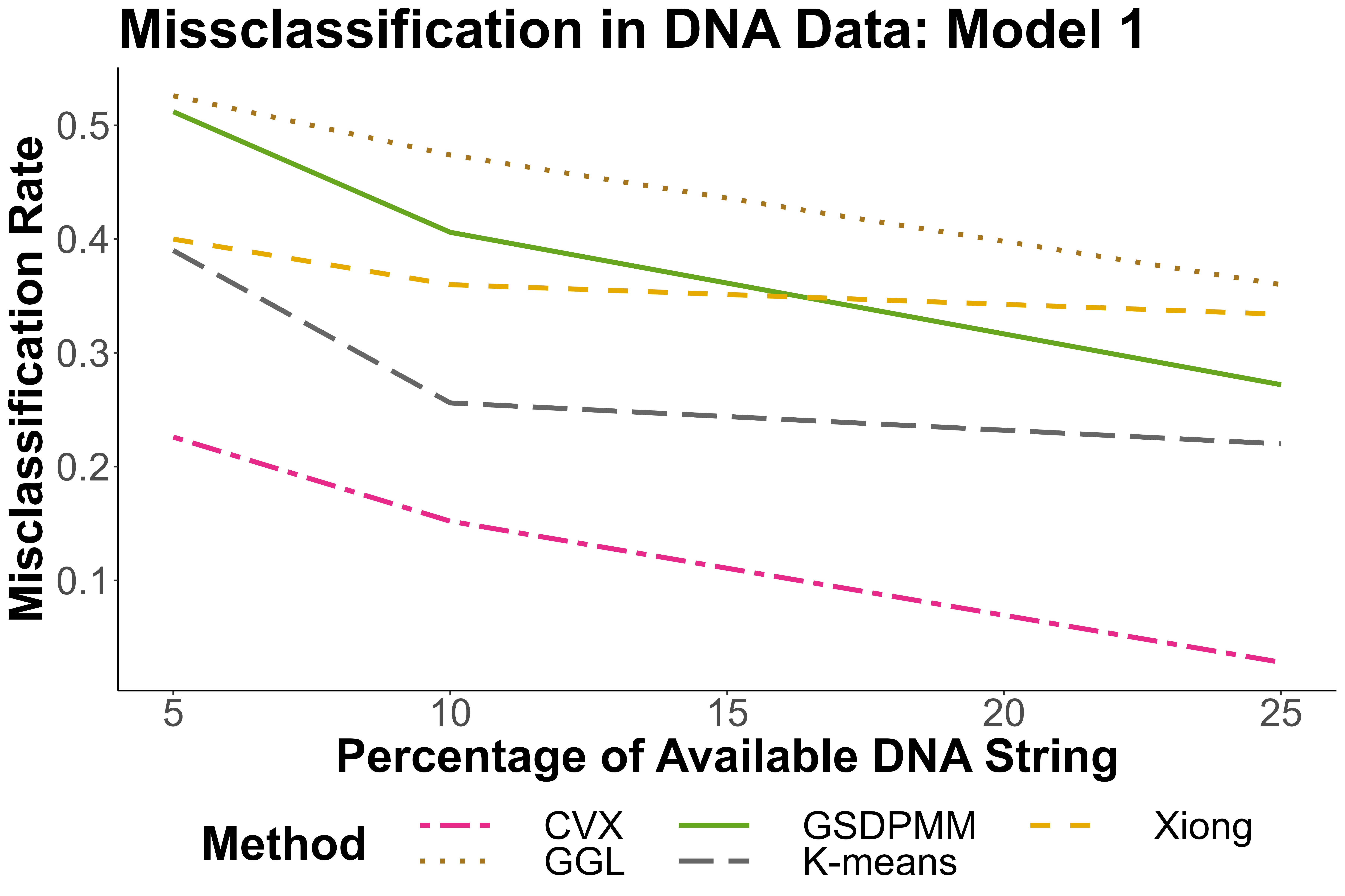
Table (2) shows the number and sizes of clusters for each reference model obtained via convex clustering. We also present the class-wise counts of the samples from a particular species in the confusion matrices in the following table (3) and report the mis-classification rates. Figure (5) compares the mis-classification rates of convex clustering with the competing methods.
| Virus | Number of Clusters | Cluster Size |
|---|---|---|
| Covid 19 | 28 | 155, 50, 10, 7, 5, 4, 2 (3 times), 1 (19 times) |
| MERS | 30 | 141, 60, 6, 5 (3 times), 3 (3 times), 2 (4 times), 1 (17 times) |
| Dengue | 7 | 24, 16, 14, 4, 3, 2, 1 |
| Hepatitis B | 14 | 41, 8, 4, 1 (11 times) |
|
MERS | Dengue |
|
Total | |||||
|---|---|---|---|---|---|---|---|---|---|
| SARS-Cov-2 | 185 | 0 | 4 | 11 | 200 | ||||
| MERS | 0 | 50 | 0 | 0 | 50 | ||||
| Dengue | 0 | 0 | 100 | 0 | 100 | ||||
| Hepatitis B | 17 | 44 | 37 | 52 | 150 |
|
MERS | Dengue |
|
Total | |||||
|---|---|---|---|---|---|---|---|---|---|
| SARS-Cov-2 | 193 | 0 | 0 | 7 | 200 | ||||
| MERS | 0 | 50 | 0 | 0 | 50 | ||||
| Dengue | 0 | 0 | 100 | 0 | 100 | ||||
| Hepatitis B | 6 | 39 | 24 | 81 | 150 |
|
MERS | Dengue |
|
Total | |||||
|---|---|---|---|---|---|---|---|---|---|
| SARS-Cov-2 | 194 | 0 | 0 | 6 | 200 | ||||
| MERS | 0 | 50 | 0 | 0 | 50 | ||||
| Dengue | 0 | 0 | 100 | 0 | 100 | ||||
| Hepatitis B | 0 | 8 | 0 | 142 | 150 |
5.3.2 Model 2
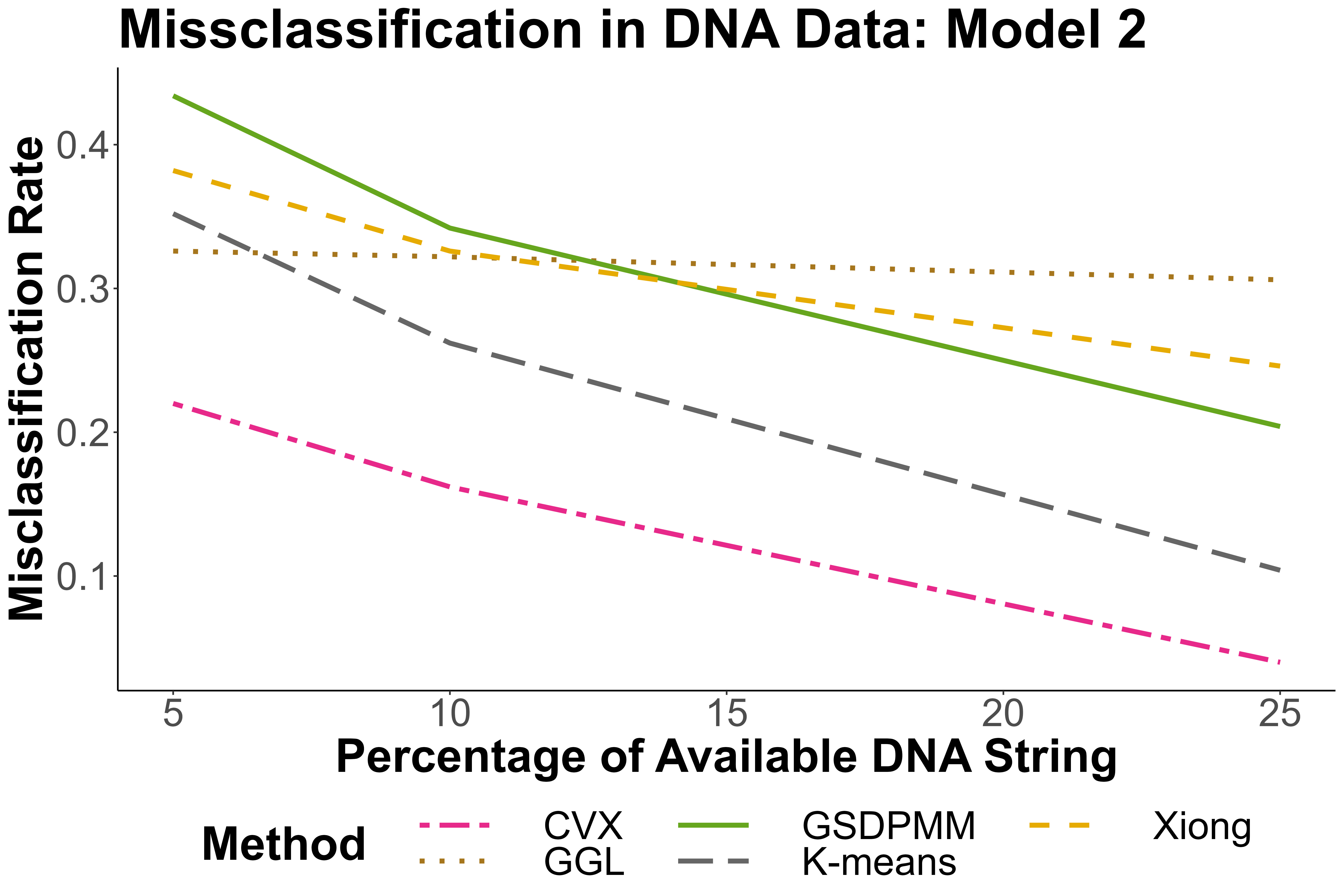
Now we present the clustering performance for the second model using convex clustering, where all fitted SMM have order in the table (4). In figure (6), we have compared the performance of convex clustering with other methods.
|
MERS | Dengue |
|
Total | |||||
|---|---|---|---|---|---|---|---|---|---|
| SARS-Cov-2 | 177 | 8 | 4 | 11 | 200 | ||||
| MERS | 1 | 49 | 0 | 0 | 50 | ||||
| Dengue | 0 | 0 | 100 | 0 | 100 | ||||
| Hepatitis B | 11 | 30 | 45 | 64 | 150 |
|
MERS | Dengue |
|
Total | |||||
|---|---|---|---|---|---|---|---|---|---|
| SARS-Cov-2 | 187 | 6 | 0 | 7 | 200 | ||||
| MERS | 0 | 50 | 0 | 0 | 50 | ||||
| Dengue | 0 | 0 | 100 | 0 | 100 | ||||
| Hepatitis B | 4 | 37 | 27 | 82 | 150 |
|
MERS | Dengue |
|
Total | |||||
|---|---|---|---|---|---|---|---|---|---|
| SARS-Cov-2 | 190 | 2 | 0 | 8 | 200 | ||||
| MERS | 0 | 50 | 0 | 0 | 50 | ||||
| Dengue | 0 | 0 | 100 | 0 | 100 | ||||
| Hepatitis B | 0 | 10 | 0 | 140 | 150 |
5.4 Discussion
In statistical analysis, larger sample sizes typically yield more reliable inference. In our experiment, when only a small portion of the genome is retained, classification performance suffers—particularly for Hepatitis B. At , the average retained segment is just 170 bases for Hepatitis B, compared to approximately 500 for Dengue and 1500 for MERS and SARS-CoV-2. This disparity explains the elevated error rate for Hepatitis B in low- settings. As the proportion of the sequence increases, accuracy improves substantially: misclassification rates fall from 22.8% to 3.2% as increases from to . Even for Hepatitis B, error drops sharply when moderately long segments are retained. For the other three viruses, misclassifications are rare across all levels.
Figures (5) and (6) confirm that convex clustering consistently outperforms other methods (GSDPMM, Xiong, GGL) across all settings. While all methods benefit from longer segments, convex clustering maintains a significant edge. At , competing methods still exceed 30% error, while convex clustering achieves rates of only 4% and 2.8% in Models 1 and 2, respectively.
Choosing the appropriate Markov order is a central issue in fitting SMMs. Higher values capture richer dependencies but risk data sparsity. For instance, setting would result in many histories with zero observations. To balance this trade-off, we select based on sequence length—using for the long genomes of SARS-CoV-2 and MERS (near 30,000 bases) and for Dengue and Hepatitis B. This empirically grounded choice ensures that most -tuples are well-represented in the data.
Beyond numerical considerations, there is a biological rationale for choosing . In DNA and RNA, three consecutive bases form a codon, which encodes either an amino acid or a stop signal during protein synthesis. Although there are 64 possible codons, they map to only 20 amino acids, with some redundancy, and a few codons act as stop signals. This triplet-based structure supports using SMMs of order at least 3 to reflect functional genomic units.
Finally, even though sequence snippets were sampled randomly from the full genomes, accurate classification was often possible. This suggests that distinctive sequence features are dispersed throughout the genome. Short segments may capture shared motifs or conserved regions (e.g., spike proteins), which can lead to mis-classification. But as sequence length increases, virus-specific patterns dominate. For example, MERS and Dengue were never misclassified by convex clustering, even at . This highlights our model’s ability to extract robust features from local sequence statistics, while the existing SMM-fitting methods fail to capture these features.
6 Summary
We proposed a convex clustering-based method for fitting sparse Markov models (SMMs), which adaptively groups transition distributions using a data-driven fusion penalty. Our approach is fully unsupervised, requiring no prior knowledge of the number of clusters or transition probabilities, and is backed by strong theoretical guarantees. In particular, we show that the true clustering structure can be consistently recovered as sample size increases, enabling efficient dimension reduction while maintaining model interpretability.
Through extensive simulation studies, we benchmarked the method against several competing approaches—GSDPMM, Xiong et al., GGL, and K-means—and found that convex clustering consistently delivers higher clustering accuracy, especially in noisy or high-dimensional settings. The method remains stable across a range of signal strengths, Markov orders, and weighting schemes, making it well-suited for general-purpose sequence modeling. The real data application to viral genomes illustrates the method’s practical relevance. Even with severely truncated sequences (e.g., retaining only 5–10% of the genome), the method accurately classifies viruses such as SARS-CoV-2, MERS, and Dengue, outperforming other methods by a substantial margin.
In summary, our method offers a statistically rigorous and computationally efficient framework for clustering and classifying sequence data under sparsity constraints. Its robustness to noise, model flexibility, and biological interpretability position it as a promising tool for applications in genomics, large language modeling, and beyond.
Acknowledgments
The authors would like to thank Dr. Iris Bennett for providing helpful code and computational suggestions, and two anonymous referees for their valuable suggestions for the improvement of the paper. They also thank the Department of Statistics, North Carolina State University for providing computing resources.
Code Availability
The R code and results for the simulation studies and real data analysis are available at: https://github.com/tuhinmajumderstat/SMM-fit-Convex-Clustering.
Data Availability
The reference and the complete genome sequences have been downloaded from the NCBI database. The exact datasets we have used can be found in this Harvard Dataverse repository. They are also available in the supplementary files with the paper.
Appendix A Proof of Theorems
A.1 Proof of Theorem 3.3
(a) For notational simplicity, we write as . Let
Suppose for some of the pairs, and . Let, . Since , we get . Also, , since the negative elements are shrunk to . Hence for any ,
Since for at least one , , contradicting that is the optimum solution. Hence , .
(b) If we initialize , we get , which satisfies . Subsequently, , and thus
. Using a similar argument, for any iteration , . Hence the limiting quantity will still have the property that the sum of the elements of is always . This completes the proof that is indeed a probability distribution.
A.2 Proof of Theorem 3.4
Note that as , . Let be the stationary probability of the state . Then, as ; and for , we have
where .
The proof mainly relies on calculating the probability of and being close to each other for all Suppose for some , and , . In that case, suppose for some , and , . In that case,
Thus, for sufficiently small, . We will later find a bound on how small needs to be to achieve this.
We compute a lower bound on the following probability:
Note that the variance-covariance matrix of the limiting distribution is not full rank, as we have a linear constraint on the elements of . Define , and let be the upper block of . Now,
Define . By the asymptotic normality of , , hence . Thus,
For a symmetric matrix matrix , Hanson and Wright 1971 have determined a lower bound on the tail probability of any quadratic form of a sub-Gaussian random variable with mean and variance-covariance matrix as follows:
| (A.6) |
for some constants . Here and are the Frobenius and spectral norms, respectively. Applying the bound in (A.6) to our problem, we obtain, as ,
As increases, , and eventually for larger , . Now,
as by the result of Watson 1996. Hence,
Now, setting , , one gets the conclusions of the theorem.
A.3 Proof of Theorem 3.5
Recall that . Denote the common transition probability for the estimated group as
Thus, the log-likelihood is given by
Note that, as increases, the number of clusters decreases. Also, by the continuity of the solution of (2.3) with respect to the , is a submodel of for as the separate clusters for lower values are clumped together to form new clusters as increases. Hence, we can write . Subsequently, . Let be the stationary probability of the state , and let be the stationary probability of the partition . Thus, . We have to show that the true model minimizes BIC with probability tending to as . We prove this for two cases.
Case 1: Suppose that and . Clearly, . Since is the true underlying model, , and
Hence, as ,
where is the approximation error such that as . The inequality follows from a lemma by Laurent and Massart 2000. If distribution, then
In our case, and we want to solve for such that . By solving the quadratic equation, we get for large . Hence the inequality holds.
Case 2: Now let and . For , without loss of generality, we can write
for . Now, as ,
and
Now, applying Jensen’s inequality by using the strict convexity of ,
Hence, , and as . Since as ,
A.4 Proof of Theorem 3.6
By definition, we can easily conclude that the weights are symmetric, hence the first part of (A1) is satisfied. Now, observe that,
Hence, for , for , and thus (A1) holds.
First, assume that the cluster sizes are different. Note that, for ,
since at most many can be non-zero if . Thus, for
and
Thus Condition (A2) holds. Now,
Also,
Hence,
A.4.1 Proof of Corollary 3.6.1
Note that (a) follows directly from the definition of and . Now if (a) holds, if , and (b) holds if , proving the result.
A.4.2 Proof of Corollary 3.6.2
Under the conditions of Theorem (3.6), for for some . If , and , then as well, since all the weights if the two -tuples and belong to different cluster. Hence, . Also, in this case if , and hence for . Thus,
and , .
Appendix B Definitions
B.1 Adjusted Rand Index
Mathematically, for any two cluster assignments and of the elements , the Rand Index is defined by
where is the number of pairs that are in the same cluster in both and , is the number of pairs that are in the different clusters in both and , is the number of pairs that are in same cluster of , but in different clusters of , and is number of pairs which are in same cluster of , but in different clusters of . Values of vary between and . If two clusters are identical, should be . Higher values indicate more similarity among two given clusters.
However, the Rand Index has some limitations. For example, if the number of clusters increases, and the cluster sizes are not large, will be close to even for two completely different cluster assignments. To address this issue, usage of the Adjusted Rand Index (ARI) is preferred. uses the expected similarity of all pairwise comparisons between clusterings specified by a random model. If , , and , then the is computed by the following formula:
Appendix C Supplementary Tables
| n | Method | Uniform Weight | Weight= | Weight= | Weylandt | |||
|---|---|---|---|---|---|---|---|---|
| knn=5 | knn=3 | knn=5 | knn=3 | |||||
| 5000 | ARI (s.e.) | 0.044 (0.137) | 0.745 (0.195) | 0.851 (0.171) | 0.720 (0.201) | 0.861 (0.170) | 0.776 (0.174) | |
|
0 | 0.223 | 0.48 | 0.187 | 0.511 | 0.267 | ||
| 10000 | ARI (s.e.) | 0.242 (0.187) | 0.946 (0.102) | 0.983 (0.056) | 0.928 (0.117) | 0.984 (0.054) | 0.960 (0.083) | |
|
0 | 0.708 | 0.908 | 0.644 | 0.908 | 0.784 | ||
| 15000 | ARI (s.e.) | 0.413 (0.189) | 0.982 (0.052) | 0.995 (0.028) | 0.974 (0.063) | 0.995 (0.028) | 0.985 (0.048) | |
|
0.001 | 0.876 | 0.972 | 0.821 | 0.973 | 0.908 | ||
| 20000 | ARI (s.e.) | 0.542 (0.191) | 0.992 (0.037) | 0.998 (0.017) | 0.989 (0.044) | 0.998 (0.017) | 0.994 (0.033) | |
|
0.008 | 0.951 | 0.991 | 0.922 | 0.99 | 0.964 | ||
| 25000 | ARI (s.e.) | 0.656 (0.179) | 0.997 (0.023) | 0.999 (0.011) | 0.994 (0.029) | 0.999 (0.011) | 0.997 (0.025) | |
|
0.028 | 0.977 | 0.996 | 0.96 | 0.996 | 0.981 | ||
| n | Method | Convex Clustering | GSDPMM | Xiong | GGL | K-means | ||
|---|---|---|---|---|---|---|---|---|
| knn=3, weight= | knn=3, weight= | |||||||
| 5000 | ARI (s.e.) | 0.851 (0.171) | 0.861 (0.17) | 0.845 (0.167) | 0.82 (0.172) | 0.413 (0.136) | 0.703 (0.216) | |
|
0.48 | 0.511 | 0.451 | 0.393 | 0.003 | 0.187 | ||
| 10000 | ARI (s.e.) | 0.983 (0.056) | 0.984 (0.054) | 0.976 (0.066) | 0.952 (0.105) | 0.706 (0.18) | 0.824 (0.201) | |
|
0.908 | 0.908 | 0.876 | 0.799 | 0.153 | 0.357 | ||
| 15000 | ARI (s.e.) | 0.995 (0.028) | 0.995 (0.028) | 0.994 (0.033) | 0.981 (0.069) | 0.876 (0.139) | 0.825 (0.199) | |
|
0.972 | 0.973 | 0.963 | 0.914 | 0.494 | 0.355 | ||
| 20000 | ARI (s.e.) | 0.998 (0.017) | 0.998 (0.017) | 0.997 (0.024) | 0.992 (0.043) | 0.943 (0.099) | 0.834 (0.194) | |
|
0.991 | 0.99 | 0.982 | 0.956 | 0.735 | 0.367 | ||
| 25000 | ARI (s.e.) | 0.999 (0.011) | 0.999 (0.011) | 0.999 (0.014) | 0.996 (0.029) | 0.975 (0.067) | 0.819 (0.199) | |
|
0.996 | 0.996 | 0.994 | 0.978 | 0.872 | 0.323 | ||
References
- Bennett et al. [2023] Iris Bennett, Donald EK Martin, and Soumendra Nath Lahiri. Fitting sparse Markov models through a collapsed gibbs sampler. Computational Statistics, 38(4):1977–1994, 2023.
- Billingsley [1961] Patrick Billingsley. Statistical methods in Markov chains. The Annals of Mathematical Statistics, pages 12–40, 1961.
- Boyd and Vandenberghe [2004] Stephen P Boyd and Lieven Vandenberghe. Convex optimization. Cambridge University Press, 2004.
- Bühlmann [2000] Peter Bühlmann. Model selection for variable length Markov chains and tuning the context algorithm. Annals of the Institute of Statistical Mathematics, 52(2):287–315, 2000.
- Bühlmann and Wyner [1999] Peter Bühlmann and Abraham J Wyner. Variable length Markov chains. The Annals of Statistics, 27(2):480–513, 1999.
- Chi and Lange [2015] Eric C Chi and Kenneth Lange. Splitting methods for convex clustering. Journal of Computational and Graphical Statistics, 24(4):994–1013, 2015.
- De Bruijn [1981] Nicolaas Govert De Bruijn. Asymptotic methods in analysis, volume 4. Courier Corporation, 1981.
- Garcıa and González-López [2011] Jesús E Garcıa and Verónica A González-López. Minimal Markov models. In Fourth Workshop on Information Theoretic Methods in Science and Engineering, page 25, 2011.
- Hanson and Wright [1971] David Lee Hanson and Farroll Tim Wright. A bound on tail probabilities for quadratic forms in independent random variables. The Annals of Mathematical Statistics, 42(3):1079–1083, 1971.
- Hocking et al. [2011] Toby Dylan Hocking, Armand Joulin, Francis Bach, and Jean-Philippe Vert. Clusterpath an algorithm for clustering using convex fusion penalties. In 28th International Conference on Machine Learning, page 1, 2011.
- Hubert and Arabie [1985] Lawrence Hubert and Phipps Arabie. Comparing partitions. Journal of Classification, 2:193–218, 1985.
- Jääskinen et al. [2014] Väinö Jääskinen, Jie Xiong, Jukka Corander, and Timo Koski. Sparse Markov chains for sequence data. Scandinavian Journal of Statistics, 41(3):639–655, 2014.
- Kontoyiannis et al. [2020] Ioannis Kontoyiannis, Lambros Mertzanis, Athina Panotopoulou, Ioannis Papageorgiou, and Maria Skoularidou. Bayesian context trees: Modelling and exact inference for discrete time series. arXiv preprint arXiv:2007.14900, 2020.
- Laurent and Massart [2000] Beatrice Laurent and Pascal Massart. Adaptive estimation of a quadratic functional by model selection. The Annals of Statistics, pages 1302–1338, 2000.
- Lindsten et al. [2011] F Lindsten, H Ohlsson, and L Ljung. Just relax and come clustering! a convexication of k-means clustering. Linköping University, Department of Electrical Engineering, Automatic Control, 2011.
- Panahi et al. [2017] Ashkan Panahi, Devdatt Dubhashi, Fredrik D Johansson, and Chiranjib Bhattacharyya. Clustering by sum of norms: Stochastic incremental algorithm, convergence and cluster recovery. In International conference on machine learning, pages 2769–2777. PMLR, 2017.
- Papageorgiou and Kontoyiannis [2022] Ioannis Papageorgiou and Ioannis Kontoyiannis. Posterior representations for Bayesian context trees: Sampling, estimation and convergence. arXiv preprint arXiv:2202.02239, 2022.
- Pelckmans et al. [2005] Kristiaan Pelckmans, Joseph De Brabanter, Johan AK Suykens, and Bart De Moor. Convex clustering shrinkage. In PASCAL Workshop on Statistics and Optimization of Clustering Workshop, 2005.
- Rissanen [1983] Jorma Rissanen. A universal prior for integers and estimation by minimum description length. The Annals of Statistics, 11(2):416–431, 1983.
- Roos and Yu [2009a] Teemu Roos and Bin Yu. Estimating sparse models from multivariate discrete data via transformed lasso. In 2009 Information Theory and Applications Workshop, pages 290–294. IEEE, 2009a.
- Roos and Yu [2009b] Teemu Roos and Bin Yu. Sparse Markov source estimation via transformed lasso. In 2009 IEEE Information Theory Workshop on Networking and Information Theory, pages 241–245. IEEE, 2009b.
- Sun et al. [2021] Defeng Sun, Kim-Chuan Toh, and Yancheng Yuan. Convex clustering: Model, theoretical guarantee and efficient algorithm. Journal of Machine Learning Research, 22:1–9, 2021.
- Wang and Allen [2021] Minjie Wang and Genevera I Allen. Integrative generalized convex clustering optimization and feature selection for mixed multi-view data. Journal of Machine Learning Research, 22:1–73, 2021.
- Watson [1996] Geoffrey S Watson. Spectral decomposition of the covariance matrix of a multinomial. Journal of the Royal Statistical Society: Series B (Methodological), 58(1):289–291, 1996.
- Weylandt et al. [2020] Michael Weylandt, John Nagorski, and Genevera I Allen. Dynamic visualization and fast computation for convex clustering via algorithmic regularization. Journal of Computational and Graphical Statistics, 29(1):87–96, 2020.
- Wu and McGoogan [2020] Zunyou Wu and Jennifer M McGoogan. Characteristics of and important lessons from the coronavirus disease 2019 (covid-19) outbreak in China: summary of a report of 72 314 cases from the chinese center for disease control and prevention. JAMA, 323(13):1239–1242, 2020.
- Xiong et al. [2016] Jie Xiong, Väinö Jääskinen, and Jukka Corander. Recursive learning for sparse Markov models. Bayesian Analysis, 11(1):247–263, 2016.
- Yuan and Lin [2006] Ming Yuan and Yi Lin. Model selection and estimation in regression with grouped variables. Journal of the Royal Statistical Society: Series B (Statistical Methodology), 68(1):49–67, 2006.
- Zhang et al. [2010] Yiyun Zhang, Runze Li, and Chih-Ling Tsai. Regularization parameter selections via generalized information criterion. Journal of the American Statistical Association, 105(489):312–323, 2010.
- Zhu et al. [2014] Changbo Zhu, Huan Xu, Chenlei Leng, and Shuicheng Yan. Convex optimization procedure for clustering: Theoretical revisit. Advances in Neural Information Processing Systems, 27, 2014.