Transverse Goldstone mode in holographic fluids with broken translations
Abstract
In this paper we investigate the low energy shear modes in fluid systems with spontaneously broken translations by a specific holographic model. In absence of momentum relaxation, we find that there exist two decoupled gapless modes in the transverse channel, one of which is purely diffusive and the other corresponds to vortex like excitations. The diffusive mode is associated with the conservation of momentum and the vortex mode can be viewed as the Goldstone mode of the spontaneous symmetry breaking. Switching on an external source which breaks the translations explicitly but weakly, the would-be gapless modes both get relaxed and acquire a tiny mass gap. Finally, in the strong momentum relaxation regime, we find a (pseudo-)diffusive-to-sound crossover that is set by a momentum gap.
I Introduction
In modern physics, symmetry principles play a crucial role in understanding laws of nature. Using the language of effective field theory (EFT), theoretical physicists have been attempting to classify and describe various different phases of condensed matter systems in terms of symmetry and symmetry breaking patterns during past few decades Nicolis et al. 2014; Nicolis et al. 2015. Such an EFT treatment has not only resulted to be very convenient for applications but also provided new insights into some widely-observed phenomena and deepened our understanding about them, for instance, the relationship between the rigidity of solids and the spontaneous breaking of spatial translations, the Goldstone nature of acoustic phonons, etc Leutwyler 1997; Alberte et al. 2019. Nevertheless, broken translations should not be viewed as a sufficient criterion for distinguishing solids from fluids in which there do not exist transverse phonons (propagating shear sound modes) due to the lack of rigidity.11 1 This statement works for low energy and long distance. However, shear propagating modes may still survive at certain short distance in fluids and the related momentum scale is called the momentum gap or “-gap”. For a detailed discussion on this, one refers to Baggioli et al. 2020a. One can manifestly show by EFT that if the system has a larger symmetry group (called the volume preserving diffeomorphisms), it can no longer resist shear deformations or mediate transverse sounds Nicolis et al. 2014; Nicolis et al. 2015. Then, questions arise that what is the difference between a fluid with spontaneously broken translations and a regular one that is translationally invariant? Since transverse sounds do not exist in the former either, what is destiny of the Goldstone modes in the transverse channel?
In this paper, we will address these questions by using the holographic method Maldacena 1998; Aharony et al. 2000; Ammon and Erdmenger 2015; Zaanen et al. 2015; Hartnoll et al. 2016; Baggioli 2019. One of the biggest advantages of holography is that the dissipative effects at finite temperature can be simply resolved by black holes in one dimension higher Policastro et al. 2001. Borrowing ideas from the EFT formulation, one can now realize breaking of translations in isotropic and homogeneous holographic models by imposing certain global internal symmetries and space-dependent configurations about several scalars in the bulk which violates the diffeomorphism invariance and gives gravitons an effective mass Vegh 2013; Blake et al. 2014. During the past few years, depending upon different setups, it has been widely investigated how the explicit breaking of translations affects the transport properties in homogeneous holographic systems Andrade and Withers 2014; Donos and Gauntlett 2014a; Donos and Gauntlett 2014b; Goutéraux 2014; Davison and Goutéraux 2015; Kim et al. 2014; Kim et al. 2015; Jeong et al. 2018; Baggioli and Pujolas 2015; Baggioli and Goykhman 2015; Alberte et al. 2016a; Baggioli and Pujolas 2017; Amoretti et al. 2016; Ling et al. 2015; Ling et al. 2016; An et al. 2020; Amoretti et al. 2021a. And more recently, it was found that even the spontaneously broken translations can be realized by choosing different UV boundary conditions in the same model which makes it possible to introduce the phonon dynamics on boundary and compare the results from holography with the experiments of cuprates Donos et al. 2018; Donos and Pantelidou 2019; Donos et al. 2019; Donos et al. 2020; Amoretti et al. 2017; Amoretti et al. 2018a; Amoretti et al. 2018b; Amoretti et al. 2019a; Amoretti et al. 2019b; Amoretti et al. 2020a; Alberte et al. 2018; Baggioli and Trachenko 2019; Ammon et al. 2019; Baggioli et al. 2019; Baggioli et al. 2020b; Amoretti et al. 2020b; Amoretti et al. 2020c; Baggioli et al. 2020c; Baggioli et al. 2020d; Pan et al. 2021; Baggioli et al. 2021a; Amoretti et al. 2021b; Wang and Li 2021; Arean et al. 2021; Wu et al. 2021. The simplest model of this type is the so-called holographic axion model in which the scalar sector satisfies an internal Euclidean symmetry (see Baggioli et al. 2021b for the most up-to-data review on this specific model). The discussions of this work will be based on a holographic charged fluid model where the spontaneously broken translations are realized by an axion-gauge coupling. It was introduced as an effective model to describe momentum relaxation effects at the beginning Goutéraux et al. 2016; Baggioli et al. 2017. However, the correct interpretation pointing to the spontaneous symmetry breaking(SSB) was unveiled in a later work Li and Wu 2019. Since the longitudinal low energy excitations in fluids are not quite different from those in solids, we will focus only on the transverse channel in this work.
The contents of the paper are organized as follows: In section II, we introduce the holographic bulk action, obtain the black hole solution and list two possible ways of breaking translations in this model, explicit and spontaneous. In section III, the transverse low energy modes are investigated both in the purely SSB case and in the pseudo-spontaneous breaking case by computing the quasi-normal modes (QNMs) of the black hole numerically. In section IV, we conclude.
II Holographic setup
In holography, fluids at finite density can be described by charged black hole geometries with one extra dimension. The simplest case is the Reisner-Nordström(RN) black hole which can be achieved from the Einstein-Maxwell action,
| (1) |
where is the Ricci scalar, is the negative cosmological constant which for simplicity is set as so that the AdS radius is normalized and with , strength of the Maxwell field that introduces a finite charge density on boundary.
In order to break the translations of the boundary system while retaining homogeneity, we couple two massless scalars (which are called axions) to the Einstein-Maxwell sector. This idea is quite similar as introducing the co-moving coordinates as dynamical fields and imposing an internal shift symmetry in the EFT formulation of solids as well as fluids Nicolis et al. 2014; Nicolis et al. 2015; Alberte et al. 2019. Then, at the lowest order in derivatives, the terms containing axions should be built in terms of
| (2) |
We expect that the dual system is a fluid and define the kinetic term of axions as follows,
| (3) |
Note that this term is just the determinant of the matrix , which satisfies the volume perserving diffeomorphisms Alberte et al. 2016a. Without loss of generality, one can also consider the axion-gauge interactions that takes the form22 2 Unlike another kind of coupling , this term does not contribute a finite shear modulus to the boundary system in the absence of external magnetic field. Therefore, the boundary system is always a fluid.
| (4) |
Then, the bulk terms containing axions can be constructed as
| (5) |
where we require that the coupling constants and so that the dual system avoids the problem of ghost Baggioli and Pujolas 2015, and obeys unitarity as well as causality Goutéraux et al. 2016.
In this model, there exists a homogeneous and isotropic black brane solution which in Eddington-Finkelstein (EF) coordinates can be expressed as
| (6) |
and
| (7) | |||
| (8) |
where and denote the boundary and horizon respectively, and correspond to the chemical potential and charge density on boundary. Note that the bulk axions are dual to boundary scalar operators . Their space dependence hence implies the breaking of translations. And the constant in (8) is a parameter characterizing the strength of the symmetry breaking. The black hole temperature and entropy density are given by
| (9) |
which should be identified as the temperature and entropy density of the dual system.
As was pointed in previous work Li and Wu 2019, near the AdS boundary , the general solution of the scalar equations can be expanded as
| (10) |
and
| (11) |
Then, in the first case above, the special solution (8) is the leading behavior of the UV expansion and plays the role of external source of the operator , following the standard quantization. On the contrary, the same solution becomes subleading in the second case and now corresponds to a non-trivial condensate which means the breaking of translations is spontaneous. In consequence, this model can easily realize different ways of the symmetry breaking via different settings on the bulk couplings.
Next, we turn to the low energy spectrum that can be achieved by investigating perturbations upon the background, and , where the quantities with bars are the background values. Without loss of generality, we choose the momentum to be parallel to the -axis. Then, the transverse modes are associated with
| (12) |
For convenience, assuming the radial gauge, i.e. , we obtain following linearized equations,
| (13) | ||||
| (14) | ||||
| (15) | ||||
| (16) | ||||
| (17) |
The UV expansions of , and close to are given by
| (18) |
Retarded Green functions can be read as
| (19) | ||||
| (20) | ||||
| (21) |
while the expression of depends on the boundary condition of axions in the UV. Then, all the correlators can be obtained once one solves (II)-(17). It is important to point out that axions do not appear in (14) explicitly. As a result of that the graviton still remains massless and33 3 The axion-gauge coupling modifies the equations of other components of gravitons. Then, it affects the thermoelectric transport in the dual system. For its impacts on the charge transport, one refers to Li and Wu 2019.
| (22) |
which implies that the shear modulus (which is defined as the real part of the stress tensor Green function at zero frequency) is vanishing. Therefore, the boundary system is indeed a fluid with the shear viscosity touching the celebrated KSS bound Kovtun et al. 2005; Alberte et al. 2016b.
In general, the excitations can be extracted directly from poles of Green functions for finite frequency and momentum. In holography, these poles coincide with the QNMs of black holes Son and Starinets 2002; Berti et al. 2009. This allows us to turn the bulk equations into secular equations with complex frequencies and real momenta, hence simplifying the numeric computation significantly.
III Low energy shear modes
From now on, we will focus on the low energy modes in the transverse channel by computing the lowest-lying QNMs. We begin our discussions with the purely SSB case, then turn to the case in the presence of an external source.
III.1 Hydrodynamic mode and frozen Goldstone mode
As was pointed out in the previous section, when we set and in the bulk, the translations are spontaneously broken. For this case, the blackening factor and the black hole temperature simply reduce to
| (23) |
which is exactly the same as the RN black hole. Based on this, QNMs of the fluctuating fields, and can be computed numerically and all the gapless modes have been plotted in Fig.1.
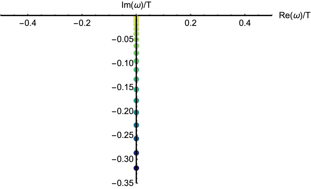
From the numeric data, there are two gapless modes: The first one is a purely diffusive mode, , where one can easily check the diffusion constant is controlled by the shear viscosity in the way that with the momentum susceptibility . Here, and are the energy density and thermodynamic pressure. Obviously, this mode is associated with the conserved total momentum and the value of perfectly matches with that in the RN black hole since the gauge-axion coupling modifies neither nor . On top of this, there is an extra gapless mode that has a trivial dispersion relation, . This mode is however absent in the RN case and should be viewed as the direct consequence of the symmetry breaking.
To manifest the existence of such a mode more, we compare our numeric result from holography with the prediction from viscoelastic hydrodynamics that is given by Amoretti et al. 2019b
| (24) |
where the shear Goldstone diffusion can be written as
| (25) |
with which in holography can be expressed as an analytic function of horizon and UV data Amoretti et al. 2019b. In the regime where is sufficiently small comparing with , the two gapless modes get decoupled as follows,
| (26) |
In fluids, the shear modulus is exactly vanishing. Then, the decoupling limit above can always be reached for arbitrary value of . As a result, the fluidity kills not only the real parts of the dispersion relations (24) but also the imaginary part of the mode in the way that as , which completely recovers the numeric result of the holographic model.44 4 Note that the derivation of the hydrodynamic result (24) is in principle based on the assumption of low frequencies and small momenta and valid to order . However, our numeric result shows that it still works very well for rather large values of . Since it is a directly consequence of the spontaneous symmetry breaking, we call the gapless mode transverse Goldstone mode in contrast to Baggioli and Grieninger 2019.
Unlike acoustic phonons, such a transverse excitation with zero gradient energy obeys the equation of motion of a quantum mechanical free particle (instead of an oscillator) whose general solution is linear in time. Thus, this can be viewed as the linearized limit of a vortex in constant rotation Endlich et al. 2011. For this reason, one can refer this kind of modes as ‘‘infinitesimal vortices” 55 5 Vortices in superfluids are gapped. On the contrary, the vortex configurations in ordinary fluids can be arbitrarily mild, involving only infinitely low momenta, which implies that these degrees of freedom should be included in the low energy description together with other gapless modes.. Since they do not feature wave or diffusive behaviors, as was verified in Gripaios and Sutherland 2015 with the field theory method that they do not appear as poles in correlators of physical observables. Moreover, the impact of the vortex on charge transport was also be investigated in holographic models with the same gauge-axion coupling Liu et al. 2022.
Another interesting issue is to check whether the diffusion constant obeys the lower bound that was proposed by Hartnoll earlier Pakhira and McKenzie 2015. Obviously, it will strongly violate the bound when we choose the butterfly velocity as the characteristic velocity Blake et al. 2017, in contrast to the crystal diffusion in the longitudinal channel Baggioli and Li 2020. However, the bound does work if the speed of sound (which is zero here) is used to bound the diffusion.
III.2 Pseudo-Goldstone mode
Now, let us consider how the two gapless modes behave when we turn on an external source that breaks translations explicitly but weakly which amounts to set in the bulk. From the field theory perspective, once the spontaneously broken symmetry is approximate, the would-be massless excitation gets slightly gapped which is now called pseudo-Goldstone. In the presence of weakly explicit breaking, the low energy poles at zero momentum can be derived using the hydrodynamic formulation Kats and Petrov 2009; Delacrétaz et al. 2017,
| (27) |
where is the rate of the momentum relaxation and denotes the phase relaxation whose origin was widely discussed in recent studies of holography Donos et al. 2021; Ammon et al. 2021 as well as effective theories Baggioli 2020; Baggioli and Landry 2020; Delacrétaz et al. 2021; Armas et al. 2021 and is called the pinning frequency related to the mass of the pseudo-Goldstone.66 6 In viscoelastic hydrodynamics, , where is the “bare mass” of the pseudo-Goldstone in its Lagrangian Delacrétaz et al. 2017. However, this formula seems not working for fluids, as it has been clearly found in some previous work that the pinning effect also exist in these systems with a zero Li and Wu 2019; Baggioli and Grieninger 2019. Solving Eq. (27) we obtain a pair of modes,
| (28) |
which are associated with the relaxed momentum and Goldstone.
For , both of the two modes are damping, lying along the imaginary axis. At , they collide on the imaginary axis, and then move off the axis when acquiring a non-trivial real part of the frequency in their dispersion relations. In the last case, we find massive excitations in the spectrum. The behavior described in (28) is in perfect agreement with what we see in the holographic model. The details have been exhibited in Fig.2.
Since the three patterns above are determined from the competition of the three parameters in (27) and (28), it is necessary to analyze how they depend upon the strength of SSB and explicit symmetry breaking(ESB). To do so, one can introduce two scales and to characterize the two kinds of symmetry breaking just as in the solid case Ammon et al. 2019. The explicit breaking of translation should be related to the mass of the spin-1 graviton
| (29) |
in the UV so that momentum is relaxed on boundary. Therefore, it is naturally to identify that
| (30) |
In the weakly broken case, i.e., , the scaling of the momentum relaxation rate can be identified as Davison and Goutéraux 2015; Hartnoll and Hofman 2012; Lucas 2015
| (31) |
Since the SSB is holographically realized by the coupling, the associated scale can be defined as
| (32) |
In the presence of both ESB and SSB, one can introduce the following dimentionless parameter for simplicity,
| (33) |
representing the ratio of the two scales. Then, the pseudo-spontaneous breaking regime implies that . In this regime, we find the following scaling of the collision point(see the right panel of Fig.2),
| (34) |
Since we set a small so that is sufficiently small comparing with the other parameters, we will neglect its effects and extract and from (28) by fitting with the numeric data. The dependence of on and has been plotted in Fig.3 and shows that
| (35) |
reminiscent of the Gell-Mann–Oaks–Renner(GMOR) relation relation firstly discovered in QCD Gell-Mann et al. 1968, and also has been touched in some studies of holography recently Andrade et al. 2018; Wang and Li 2021.
Moreover, the scaling of the phase relaxation
| (36) |
has also been shown in Fig.4. Then, in the pseudo-spontaneous regime with , we have
| (37) |
which means the pinning frequency dominates the real part of (28), therefore can be treated as the physical mass of the pseudo-Goldstone modes.
III.3 Dispersion relation and k-gap
In the final subsection, we will discuss the dispersion relations of the shear modes for finite momentum. The numeric result has been displayed in Fig.5. We also start the dicussions with the pseudo-spontaneous case, i.e., supposing is sufficiently large. We find that the dispersion relations of pseudo-Goldstone modes for small are given by
| (38) |
in the pseudo-spontaneous regime. Apart from the real part, imaginary part has a pseudo-diffusive like scaling which implies that the pseudo-Goldstone is coupled with the momentum and may have a contribution to the transport. This is different from the purely SSB case where the Goldstone is completed frozen. When is large and increased, these two modes move towards the imaginary axis of the frequency, collide, split and move in the opposite directions on the imaginary axis again.
Moreover, if we increase more and more, the pseudo-spontaneous breaking pattern breaks down duo the significant effect of . Meanwhile, the mass of the pseudo-Goldstones get smaller and smaller. When the value of is down to certain critical value , two sound modes emerge. These two modes are, nevertheless, a result of fine-tuning. Once we increase further, they will be destroyed and become pseudo-diffusive at low momenta and propagating at high momenta which is similar as the purely explicit breaking pattern Davison and Goutéraux 2015; Kim et al. 2014. In this case, the associated value of momentum that separates the two behaviors is called a k-gap. Scalings of the emergent sound speed and have been fixed by the data in Fig.6,
| (39) |
However, the origin of such an emergent sound speed due to the ESB of translations still remains mysterious.
IV Conclusions
In this paper, we investigate low energy transverse excitations of a simple holographic fluid model with spontaneous broken translations. In the purely spontaneous breaking case, there are two decoupled gapless shear modes one of which is diffusive and associated with the conserved momentum. The other is the Goldstone mode of the symmetry breaking that behaves like gapless vortices.
Then, we switch on an external source to break the translations also explicitly. When the effect of momentum relaxation is weak, the would-be gapless modes are coupled and form a pair of slightly gapped pseudo-Goldstone modes via colliding on the imaginary axis of frequency. We verify that the mass of the pseudo-Goldstone modes satisfies the GMOR relation. Their lifetime is characterized by the phase relaxation which comes from breaking simultaneously the translations and global internal shift symmetry Ammon et al. 2021. When the momentum relaxation is strong enough, we find that the picture of pseudo-Goldstones breaks down and the mass of the shear modes becomes smaller as the increase of the relaxation rate. Finally, they become massless and generate a -gap that sets a (pseudo-)diffusion-to-sound crossover which is similar as the purely ESB case.
Acknowledgments
We would like to thank Matteo Baggioli for numerous helpful discussions on (pseudo-) Goldstone modes in fluids and Xi-Jing Wang for sharing his experience in numerical calculations. This work is supported by NSFC No.11905024.
References
- Nicolis et al. (2014) A. Nicolis, R. Penco, and R. A. Rosen, Phys. Rev. D 89, 045002 (2014), arXiv:1307.0517 [hep-th] .
- Nicolis et al. (2015) A. Nicolis, R. Penco, F. Piazza, and R. Rattazzi, JHEP 06, 155 (2015), arXiv:1501.03845 [hep-th] .
- Leutwyler (1997) H. Leutwyler, Helv. Phys. Acta 70, 275 (1997), arXiv:hep-ph/9609466 .
- Alberte et al. (2019) L. Alberte, M. Baggioli, V. C. Castillo, and O. Pujolas, Phys. Rev. D 100, 065015 (2019), [Erratum: Phys.Rev.D 102, 069901 (2020)], arXiv:1807.07474 [hep-th] .
- Baggioli et al. (2020a) M. Baggioli, M. Vasin, V. V. Brazhkin, and K. Trachenko, Phys. Rept. 865, 1 (2020a), arXiv:1904.01419 [cond-mat.stat-mech] .
- Maldacena (1998) J. M. Maldacena, Adv. Theor. Math. Phys. 2, 231 (1998), arXiv:hep-th/9711200 .
- Aharony et al. (2000) O. Aharony, S. S. Gubser, J. M. Maldacena, H. Ooguri, and Y. Oz, Phys. Rept. 323, 183 (2000), arXiv:hep-th/9905111 .
- Ammon and Erdmenger (2015) M. Ammon and J. Erdmenger, Gauge/gravity duality: Foundations and applications (Cambridge University Press, Cambridge, 2015).
- Zaanen et al. (2015) J. Zaanen, Y.-W. Sun, Y. Liu, and K. Schalm, Holographic Duality in Condensed Matter Physics (Cambridge Univ. Press, 2015).
- Hartnoll et al. (2016) S. A. Hartnoll, A. Lucas, and S. Sachdev, (2016), arXiv:1612.07324 [hep-th] .
- Baggioli (2019) M. Baggioli, Applied Holography: A Practical Mini-Course, SpringerBriefs in Physics (Springer, 2019) arXiv:1908.02667 [hep-th] .
- Policastro et al. (2001) G. Policastro, D. T. Son, and A. O. Starinets, Phys. Rev. Lett. 87, 081601 (2001), arXiv:hep-th/0104066 .
- Vegh (2013) D. Vegh, (2013), arXiv:1301.0537 [hep-th] .
- Blake et al. (2014) M. Blake, D. Tong, and D. Vegh, Phys. Rev. Lett. 112, 071602 (2014), arXiv:1310.3832 [hep-th] .
- Andrade and Withers (2014) T. Andrade and B. Withers, JHEP 05, 101 (2014), arXiv:1311.5157 [hep-th] .
- Donos and Gauntlett (2014a) A. Donos and J. P. Gauntlett, JHEP 04, 040 (2014a), arXiv:1311.3292 [hep-th] .
- Donos and Gauntlett (2014b) A. Donos and J. P. Gauntlett, JHEP 11, 081 (2014b), arXiv:1406.4742 [hep-th] .
- Goutéraux (2014) B. Goutéraux, JHEP 04, 181 (2014), arXiv:1401.5436 [hep-th] .
- Davison and Goutéraux (2015) R. A. Davison and B. Goutéraux, JHEP 01, 039 (2015), arXiv:1411.1062 [hep-th] .
- Kim et al. (2014) K.-Y. Kim, K. K. Kim, Y. Seo, and S.-J. Sin, JHEP 12, 170 (2014), arXiv:1409.8346 [hep-th] .
- Kim et al. (2015) K.-Y. Kim, K. K. Kim, and M. Park, JHEP 04, 152 (2015), arXiv:1501.00446 [hep-th] .
- Jeong et al. (2018) H.-S. Jeong, Y. Ahn, D. Ahn, C. Niu, W.-J. Li, and K.-Y. Kim, JHEP 01, 140 (2018), arXiv:1708.08822 [hep-th] .
- Baggioli and Pujolas (2015) M. Baggioli and O. Pujolas, Phys. Rev. Lett. 114, 251602 (2015), arXiv:1411.1003 [hep-th] .
- Baggioli and Goykhman (2015) M. Baggioli and M. Goykhman, JHEP 07, 035 (2015), arXiv:1504.05561 [hep-th] .
- Alberte et al. (2016a) L. Alberte, M. Baggioli, A. Khmelnitsky, and O. Pujolas, JHEP 02, 114 (2016a), arXiv:1510.09089 [hep-th] .
- Baggioli and Pujolas (2017) M. Baggioli and O. Pujolas, JHEP 01, 040 (2017), arXiv:1601.07897 [hep-th] .
- Amoretti et al. (2016) A. Amoretti, M. Baggioli, N. Magnoli, and D. Musso, JHEP 06, 113 (2016), arXiv:1603.03029 [hep-th] .
- Ling et al. (2015) Y. Ling, P. Liu, C. Niu, and J.-P. Wu, Phys. Rev. D 92, 086003 (2015), arXiv:1507.02514 [hep-th] .
- Ling et al. (2016) Y. Ling, Z.-Y. Xian, and Z. Zhou, JHEP 11, 007 (2016), arXiv:1605.03879 [hep-th] .
- An et al. (2020) Y.-S. An, T. Ji, and L. Li, JHEP 10, 023 (2020), arXiv:2007.13918 [hep-th] .
- Amoretti et al. (2021a) A. Amoretti, D. Arean, D. K. Brattan, and L. Martinoia, JHEP 11, 011 (2021a), arXiv:2107.00519 [hep-th] .
- Donos et al. (2018) A. Donos, J. P. Gauntlett, T. Griffin, and V. Ziogas, JHEP 04, 053 (2018), arXiv:1801.09084 [hep-th] .
- Donos and Pantelidou (2019) A. Donos and C. Pantelidou, JHEP 05, 079 (2019), arXiv:1903.05114 [hep-th] .
- Donos et al. (2019) A. Donos, D. Martin, C. Pantelidou, and V. Ziogas, JHEP 10, 218 (2019), arXiv:1905.00398 [hep-th] .
- Donos et al. (2020) A. Donos, D. Martin, C. Pantelidou, and V. Ziogas, Class. Quant. Grav. 37, 045005 (2020), arXiv:1906.03132 [hep-th] .
- Amoretti et al. (2017) A. Amoretti, D. Areán, R. Argurio, D. Musso, and L. A. Pando Zayas, JHEP 05, 051 (2017), arXiv:1611.09344 [hep-th] .
- Amoretti et al. (2018a) A. Amoretti, D. Areán, B. Goutéraux, and D. Musso, Phys. Rev. D 97, 086017 (2018a), arXiv:1711.06610 [hep-th] .
- Amoretti et al. (2018b) A. Amoretti, D. Areán, B. Goutéraux, and D. Musso, Phys. Rev. Lett. 120, 171603 (2018b), arXiv:1712.07994 [hep-th] .
- Amoretti et al. (2019a) A. Amoretti, D. Areán, B. Goutéraux, and D. Musso, Phys. Rev. Lett. 123, 211602 (2019a), arXiv:1812.08118 [hep-th] .
- Amoretti et al. (2019b) A. Amoretti, D. Areán, B. Goutéraux, and D. Musso, JHEP 10, 068 (2019b), arXiv:1904.11445 [hep-th] .
- Amoretti et al. (2020a) A. Amoretti, D. Areán, B. Goutéraux, and D. Musso, JHEP 01, 058 (2020a), arXiv:1910.11330 [hep-th] .
- Alberte et al. (2018) L. Alberte, M. Ammon, A. Jiménez-Alba, M. Baggioli, and O. Pujolàs, Phys. Rev. Lett. 120, 171602 (2018), arXiv:1711.03100 [hep-th] .
- Baggioli and Trachenko (2019) M. Baggioli and K. Trachenko, JHEP 03, 093 (2019), arXiv:1807.10530 [hep-th] .
- Ammon et al. (2019) M. Ammon, M. Baggioli, and A. Jiménez-Alba, JHEP 09, 124 (2019), arXiv:1904.05785 [hep-th] .
- Baggioli et al. (2019) M. Baggioli, U. Gran, A. J. Alba, M. Tornsö, and T. Zingg, JHEP 09, 013 (2019), arXiv:1905.00804 [hep-th] .
- Baggioli et al. (2020b) M. Baggioli, S. Grieninger, and H. Soltanpanahi, Phys. Rev. Lett. 124, 081601 (2020b), arXiv:1910.06331 [hep-th] .
- Amoretti et al. (2020b) A. Amoretti, M. Meinero, D. K. Brattan, F. Caglieris, E. Giannini, M. Affronte, C. Hess, B. Buechner, N. Magnoli, and M. Putti, Phys. Rev. Res. 2, 023387 (2020b), arXiv:1909.07991 [cond-mat.str-el] .
- Amoretti et al. (2020c) A. Amoretti, D. K. Brattan, N. Magnoli, and M. Scanavino, JHEP 08, 097 (2020c), arXiv:2005.09662 [hep-th] .
- Baggioli et al. (2020c) M. Baggioli, S. Grieninger, and L. Li, JHEP 09, 037 (2020c), arXiv:2005.01725 [hep-th] .
- Baggioli et al. (2020d) M. Baggioli, V. C. Castillo, and O. Pujolas, JHEP 09, 013 (2020d), arXiv:2006.10774 [hep-th] .
- Pan et al. (2021) D. Pan, T. Ji, M. Baggioli, L. Li, and Y. Jin, (2021), arXiv:2108.13124 [cond-mat.soft] .
- Baggioli et al. (2021a) M. Baggioli, L. Li, and H.-T. Sun, (2021a), arXiv:2112.14855 [hep-th] .
- Amoretti et al. (2021b) A. Amoretti, D. Arean, D. K. Brattan, and N. Magnoli, JHEP 05, 027 (2021b), arXiv:2101.05343 [hep-th] .
- Wang and Li (2021) X.-J. Wang and W.-J. Li, JHEP 07, 131 (2021), arXiv:2105.07225 [hep-th] .
- Arean et al. (2021) D. Arean, R. A. Davison, B. Goutéraux, and K. Suzuki, Phys. Rev. X 11, 031024 (2021), arXiv:2011.12301 [hep-th] .
- Wu et al. (2021) N. Wu, M. Baggioli, and W.-J. Li, JHEP 05, 014 (2021), arXiv:2102.05810 [hep-th] .
- Baggioli et al. (2021b) M. Baggioli, K.-Y. Kim, L. Li, and W.-J. Li, Sci. China Phys. Mech. Astron. 64, 270001 (2021b), arXiv:2101.01892 [hep-th] .
- Goutéraux et al. (2016) B. Goutéraux, E. Kiritsis, and W.-J. Li, JHEP 04, 122 (2016), arXiv:1602.01067 [hep-th] .
- Baggioli et al. (2017) M. Baggioli, B. Goutéraux, E. Kiritsis, and W.-J. Li, JHEP 03, 170 (2017), arXiv:1612.05500 [hep-th] .
- Li and Wu (2019) W.-J. Li and J.-P. Wu, Eur. Phys. J. C 79, 243 (2019), arXiv:1808.03142 [hep-th] .
- Kovtun et al. (2005) P. Kovtun, D. T. Son, and A. O. Starinets, Phys. Rev. Lett. 94, 111601 (2005), arXiv:hep-th/0405231 .
- Alberte et al. (2016b) L. Alberte, M. Baggioli, and O. Pujolas, JHEP 07, 074 (2016b), arXiv:1601.03384 [hep-th] .
- Son and Starinets (2002) D. T. Son and A. O. Starinets, JHEP 09, 042 (2002), arXiv:hep-th/0205051 .
- Berti et al. (2009) E. Berti, V. Cardoso, and A. O. Starinets, Class. Quant. Grav. 26, 163001 (2009), arXiv:0905.2975 [gr-qc] .
- Baggioli and Grieninger (2019) M. Baggioli and S. Grieninger, JHEP 10, 235 (2019), arXiv:1905.09488 [hep-th] .
- Endlich et al. (2011) S. Endlich, A. Nicolis, R. Rattazzi, and J. Wang, JHEP 04, 102 (2011), arXiv:1011.6396 [hep-th] .
- Gripaios and Sutherland (2015) B. Gripaios and D. Sutherland, Phys. Rev. Lett. 114, 071601 (2015), arXiv:1406.4422 [hep-th] .
- Liu et al. (2022) Y. Liu, X.-J. Wang, J.-P. Wu, and X. Zhang, (2022), arXiv:2201.06065 [hep-th] .
- Pakhira and McKenzie (2015) N. Pakhira and R. H. McKenzie, Physical Review B 91 (2015), 10.1103/physrevb.91.075124.
- Blake et al. (2017) M. Blake, R. A. Davison, and S. Sachdev, Phys. Rev. D 96, 106008 (2017), arXiv:1705.07896 [hep-th] .
- Baggioli and Li (2020) M. Baggioli and W.-J. Li, SciPost Phys. 9, 007 (2020), arXiv:2005.06482 [hep-th] .
- Kats and Petrov (2009) Y. Kats and P. Petrov, JHEP 01, 044 (2009), arXiv:0712.0743 [hep-th] .
- Delacrétaz et al. (2017) L. V. Delacrétaz, B. Goutéraux, S. A. Hartnoll, and A. Karlsson, Phys. Rev. B 96, 195128 (2017), arXiv:1702.05104 [cond-mat.str-el] .
- Donos et al. (2021) A. Donos, P. Kailidis, and C. Pantelidou, JHEP 09, 134 (2021), arXiv:2107.03680 [hep-th] .
- Ammon et al. (2021) M. Ammon, D. Arean, M. Baggioli, S. Gray, and S. Grieninger, (2021), arXiv:2111.10305 [hep-th] .
- Baggioli (2020) M. Baggioli, Phys. Rev. Res. 2, 022022 (2020), arXiv:2001.06228 [hep-th] .
- Baggioli and Landry (2020) M. Baggioli and M. Landry, SciPost Phys. 9, 062 (2020), arXiv:2008.05339 [hep-th] .
- Delacrétaz et al. (2021) L. V. Delacrétaz, B. Goutéraux, and V. Ziogas, (2021), arXiv:2111.13459 [hep-th] .
- Armas et al. (2021) J. Armas, A. Jain, and R. Lier, (2021), arXiv:2112.14373 [hep-th] .
- Hartnoll and Hofman (2012) S. A. Hartnoll and D. M. Hofman, Phys. Rev. Lett. 108, 241601 (2012), arXiv:1201.3917 [hep-th] .
- Lucas (2015) A. Lucas, JHEP 03, 071 (2015), arXiv:1501.05656 [hep-th] .
- Gell-Mann et al. (1968) M. Gell-Mann, R. J. Oakes, and B. Renner, Phys. Rev. 175, 2195 (1968).
- Andrade et al. (2018) T. Andrade, M. Baggioli, A. Krikun, and N. Poovuttikul, JHEP 02, 085 (2018), arXiv:1708.08306 [hep-th] .