Understanding Curriculum Learning in Policy Optimization for Online Combinatorial Optimization
Abstract
Over the recent years, reinforcement learning (RL) starts to show promising results in tackling combinatorial optimization (CO) problems, in particular when coupled with curriculum learning to facilitate training. Despite emerging empirical evidence, theoretical study on why RL helps is still at its early stage. This paper presents the first systematic study on policy optimization methods for online CO problems. We show that online CO problems can be naturally formulated as latent Markov Decision Processes (LMDPs), and prove convergence bounds on natural policy gradient (NPG) for solving LMDPs. Furthermore, our theory explains the benefit of curriculum learning: it can find a strong sampling policy and reduce the distribution shift, a critical quantity that governs the convergence rate in our theorem. For a canonical online CO problem, the Best Choice Problem (BCP), we formally prove that distribution shift is reduced exponentially with curriculum learning even if the curriculum is a randomly generated BCP on a smaller scale. Our theory also shows we can simplify the curriculum learning scheme used in prior work from multi-step to single-step. Lastly, we provide extensive experiments on the Best Choice Problem, Online Knapsack, and AdWords to verify our findings.
1 Introduction
In recent years, machine learning techniques have shown promising results in solving combinatorial optimization (CO) problems, including traveling salesman problem (TSP, Kool et al. 2019), maximum cut (Khalil et al. 2017) and satisfiability problem (Selsam et al. 2019). While in the worst case some CO problems are NP-hard, in practice, the probability that we need to solve the worst-case problem instance is low (Cappart et al. 2021). Machine learning techniques are able to find generic models which have exceptional performance on the majority of a class of CO problems.
A significant subclass of CO problems is called online CO problems, which has gained much attention (Grötschel et al. 2001; Huang 2019; Garg et al. 2008). Online CO problems entail a sequential decision-making process, which perfectly matches the nature of reinforcement learning (RL).
This paper concerns using RL to tackle online CO problems. RL is often coupled with specialized techniques including (a particular type of) Curriculum Learning (Kong et al. 2019), human feedback and correction (Pérez-Dattari et al. 2018, Scholten et al. 2019), and policy aggregation (boosting, Brukhim et al. 2021). Practitioners use these techniques to accelerate the training speed.
While these hybrid techniques enjoy empirical success, the theoretical understanding is still limited: it is unclear when and why they improve the performance. In this paper, we particularly focus on RL with Curriculum Learning (Bengio et al. 2009, also named “bootstrapping” in Kong et al. 2019): train the agent from an easy task and gradually increase the difficulty until the target task. Interestingly, these techniques exploit the special structures of online CO problems.
Main contributions. In this paper, we initiate the formal study on using RL to tackle online CO problems, with a particular emphasis on understanding the specialized techniques developed in this emerging subarea. Our contributions are summarized below.
Formalization. For online CO problems, we want to learn a single policy that enjoys good performance over a distribution of problem instances. This motivates us to use Latent Markov Decision Process (LMDP) (Kwon et al. 2021a) instead of standard MDP formulation. We give concrete examples, the Best Choice Problem (BCP, also known as the Secretary Problem), Online Knapsack, and AdWords (Online Matching and Ad Allocation, ADW), to show how LMDP models online CO problems. With this formulation, we can systematically analyze RL algorithms.
Provable efficiency of policy optimization. By leveraging recent theory on Natural Policy Gradient for standard MDP Agarwal et al. 2021, we analyze the performance of NPG for LMDP. The performance bound is characterized by the number of iterations, the excess risk of policy evaluation, the transfer error, and the relative condition number that characterizes the distribution shift between the sampling policy and the optimal policy. We also take into account the effect of entropy regularization. To our knowledge, this is the first performance bound of policy optimization methods on LMDP.
Understanding and simplifying Curriculum Learning. Using our performance guarantee on NPG for LMDP, we study when and why Curriculum Learning is beneficial to RL for online CO problems. Our main finding is that the main effect of Curriculum Learning is to give a stronger sampling policy. Under certain circumstances, Curriculum Learning reduces the relative condition number , improving the convergence rate. For BCP, we provably show that Curriculum Learning can exponentially reduce compared with using the naïve sampling policy. Surprisingly, this means even a randomly constructed curriculum of BCP accelerates the training exponentially. As a direct implication, we show that the multi-step Curriculum Learning proposed in Kong et al. 2019 can be significantly simplified into a single-step scheme. Lastly, to obtain a complete understanding, we study the failure mode of Curriculum Learning, in a way to help practitioners to decide whether to use Curriculum Learning based on their prior knowledge. To verify our theories, we conduct extensive experiments on three classical online CO problems [BCP, Online Knapsack (decision version, OKD), and ADW (decision version)] and carefully track the dependency between the performance of the policy and .
2 Related Works
Combinatorial Optimization problems. CO has been a long lasting field of people’s interest. There are a rich literature regarding CO problems such as traveling salesman problem (Flood 1956; Bellmore & Nemhauser 1968), maximum cut (Karp 1972; Goemans & Williamson 1995), and satisfiability problem (Cook 1971; Trakhtenbrot 1984).
RL for CO. There have been rich literature studying RL for CO problems, e.g., using Pointer Network in REINFORCE and Actor-Critic for routing problems (Nazari et al. 2018), combining Graph Attention Network with Monte Carlo Tree Search for TSP (Drori et al. 2020) and incorporating Structure-to-Vector Network in Deep Q-networks for maximum independent set problems (Cappart et al. 2019). Bello et al. 2017 proposed a framework to tackle CO problems using RL and neural networks. Kool et al. 2019 combined REINFORCE and attention technique to learn routing problems. Vesselinova et al. 2020 and Mazyavkina et al. 2021 are taxonomic surveys of RL approaches for graph problems. Bengio et al. 2020 summarized learning methods, algorithmic structures, objective design and discussed generalization. In particular scaling to larger problems was mentioned as a major challenge. Compared to supervised learning, RL not only mimics existing heuristics, but also discover novel ones that humans have not thought of, for example chip design (Mirhoseini et al. 2021) and compiler optimization (Zhou et al. 2020b). Theoretically, there is a line of work on analyzing data-driven approach to combinatorial problems (Balcan 2020). However, to our knowledge, the theoretical analysis for RL-based method is still missing.
Kong et al. 2019 focused on using RL to tackle online CO problems, which means that the agent must make sequential and irrevocable decisions. They encoded the input in a length-independent manner. For example, the -th element of a -length sequence is encoded by the fraction and other features, so that the agent can generalize to unseen , paving the way for Curriculum Learning. Three online CO problems were mentioned in their paper: ADW, Online Knapsack, and BCP. Currently, Online Matching (ADW) and Online Knapsack have only approximation algorithms (Huang et al. 2019; Albers et al. 2021). There are also other works about RL for online CO problems. Alomrani et al. 2021 uses deep-RL for Online Matching. Oren et al. 2021 studies Parallel Machine Job Scheduling problem (PMSP) and Capacitated Vehicle Routing problem (CVRP), which are both online CO problems, using offline-learning and Monte Carlo Tree Search.
LMDP. We provide the exact definition of LMDP in Section 4.1. As studied by Steimle et al. 2021, in the general cases, optimal policies for LMDPs are history-dependent. This is different from standard MDP cases where there always exists an optimal history-independent policy. They showed that even finding the optimal history-independent policy is NP-hard. Kwon et al. 2021a investigated the sample complexity and regret bounds of LMDP in the history-independent policy class. They presented an exponential lower-bound for a general LMDP and derived algorithms with polynomial sample complexities for cases with special assumptions. Kwon et al. 2021b showed that in reward-mixing MDPs, where MDPs share the same transition model, a polynomial sample complexity is achievable without any assumption to find an optimal history-independent policy.
Convergence rate for policy gradient methods. There is line of work on the convergence rates of policy gradient methods for standard MDPs (Bhandari & Russo 2021, Wang et al. 2020, Liu et al. 2020, Ding et al. 2021, Zhang et al. 2021). For softmax tabular parameterization, NPG can obtain an rate (Agarwal et al. 2021) where is the number of iterations; with entropy regularization, both PG and NPG achieves linear convergence (Mei et al. 2020; Cen et al. 2021). For log-linear policies, sample-based NPG makes an convergence rate, with assumptions on and (Agarwal et al. 2021) (see our Definition 4); exact NPG with entropy regularization enjoys a linear convergence rate up to (Cayci et al. 2021). We extend the analysis to LMDP.
Curriculum Learning. There are a rich body of literature on Curriculum Learning (Zhou et al. 2021b; Zhou et al. 2021a; Zhou et al. 2020a; Ao et al. 2021; Willems et al. 2020; Graves et al. 2017). As surveyed in Bengio et al. 2009, Curriculum Learning has been applied to training deep neural networks and non-convex optimizations and improves the convergence in several cases. Narvekar et al. 2020 rigorously modeled curriculum as a directed acyclic graph and surveyed work on curriculum design. Kong et al. 2019 proposed a bootstrapping (Curriculum Learning) approach: gradually increase the problem size after the model works sufficiently well on the current problem size.
3 Motivating Online CO Problems
Online CO problems are a natural class of problems that admit constructions of small-scale instances, because the hardness of them can be characterized by the input length, and instances of different scales are similar. This property simplifies the construction of curricula and underscores curriculum learning. We also believe online CO problems make the use of LMDP suitable, because under a proper distribution , instances in a large portion of the probability space have similar near optimal solutions.
In this section we introduce three motivating online CO problems. We are interested in these problems because they have all been extensively studied. Furthermore, they were studied in Kong et al. 2019, the paper that motivates our work. They also have real-world applications, e.g., auction design (Babaioff et al. 2007) and advertisement targeting (Mehta et al. 2007).
3.1 The Best Choice Problem (BCP)11 1 We follow the statement in Kong et al. 2019 that BCP (secretary problem) is a CO problem. It is categorized as an optimal stopping problem.
In BCP, the goal is to maximize the probability of choosing the maximum among different numbers, where is known. They arrive sequentially and when the -th number shows up, the decision-maker observes the relative ranking among the first numbers, which means being the th-best so far. A decision that whether to accept or reject the -th number must be made immediately when it comes, and such decisions cannot be revoked. Once one number is accepted, the game ends immediately.
The ordering of the numbers is unknown. There are in total permutations, and an instance of BCP is drawn from an unknown distribution over these permutations. In the classical BCP, each permutation is sampled with equal probability. The optimal solution for the classical BCP is the well-known -threshold strategy: reject all the first numbers, then accept the first one which is the best so-far. In this paper, we also study some different distributions.
3.2 Online Knapsack (decision version, OKD)
In Online Knapsack problems the decision-maker observes (which is known) items arriving sequentially, each with value and size revealed upon arrival. A decision to either accept or reject the -th item must be made immediately when it arrives, and such decisions cannot be revoked. At any time the accepted items should have their total size no larger than a known budget .
The goal of standard Online Knapsack is to maximize the total value of accepted items. In this paper, we study its decision version, whose goal is to maximize the probability of total value reaching a known target .
We assume that all values and sizes are sampled independently from two fixed distributions, namely and . In Kong et al. 2019 the experiments were carried out with , and we also study other distributions.
Remark 1.
A challenge in OKD is the sparse reward: the only signal is reward when the total value of accepted items first exceeds (see the detailed formulation in Section C.2), unlike in Online Knapsack the reward of is given instantly after the -th item is successfully accepted. This makes random exploration hardly get reward signals, necessitating Curriculum Learning.
3.3 AdWords (decision version, ADW)
In ADW, there are advertisers each with budget and ad slots. Each ad slot arrives sequentially along with a vector where is the value that advertiser wants to pay for ad slot . Once an ad slot arrives, it must be irrevocably allocated to an advertiser or not allocated at all. If ad slot is allocated to advertiser and the remaining budget of advertiser is not less than , the total revenue increases by while advertiser ’s budget decreases by .
We assume that for any advertiser , . Kong et al. 2019 studied a very special case called online -matching where is a Bernoulli distribution. We study different distributions.
The objective of the standard ADW is to maximize the total revenue. For a similar reason as in OKD, we set a known target for the decision version. The goal of ADW is to maximize the probability of total revenue reaching .
4 Problem Setup
In this section, we first introduce LMDP and why it naturally formulates online CO problems. Then we list necessary components required by Natural Policy Gradient for LMDP (Algorithm 1).
Notations.
For any positive integer , we denote . For any vector , we denote as the self-outer-product of . Further for any , we denote .
4.1 Latent Markov Decision Process
Tackling an online CO problem entails handling a family of problem instances, and each instance can be modeled as a Markov Decision Process. For online CO problems, we want to find one algorithm that works for a family of problem instances and performs well on average over an (unknown) distribution over this family. To this end, we adopt the concept of Latent MDP which naturally models online CO problems.
Latent MDP (Kwon et al. 2021a) is a collection of MDPs . All the MDPs share state set , action set and horizon . Each MDP has its own initial state distribution , transition and reward , where is the probability simplex over . Let be the mixing weights of MDPs such that for any and . At the start of every episode, one MDP is randomly chosen with probability .
Due to the time and space complexities of finding the optimal history-dependent policies, we stay in line with Kong et al. 2019 and care only about finding the optimal history-independent policy. Let denote the class of all the history-independent policies.
Log-linear policy. Let be a feature mapping function where denotes the dimension of feature space. Assume that . A log-linear policy is of the form:
Remark 2.
Log-linear parameterization is a generalization of softmax tabular parameterization by setting and One-hot. They are “scalable”: if extracts important features from different s with a fixed dimension , then a single can generalize.
Value function, Q-function and advantage function. The expected reward of executing on is defined via value functions. We incorporate entropy regularization for completeness because prior works (especially empirical works) used it to facilitate training. Due to space limit, we defer all the entropy regularized notations, algorithm and theorem to Appendix A. We define the value function:
where the expectation is with respect to the randomness of trajectory induced by in . Denote , then we need to find . Denote .
The Q-function can be defined in a similar manner:
and the advantage function is defined as .
Modeling BCP. For BCP, each instance is a permutation of length , and in each round an instance is drawn from an unknown distribution over all permutations. In the -th step for , the state encodes the -th number and its relative ranking so far. The transition is deterministic according to the problem definition. A reward of is given if and only if the maximum is accepted. We model the distribution as follows: for the -th number, it has probability to be the best so-far and is independent of other . Hence, the weight of each instance is simply the product of the probabilities on each position. The classical BCP satisfies .
Modeling OKD. For OKD, each instance is a sequence of items with values and sizes drawn from unknown distributions and . In the -th step for , the state encodes the information of -th item’s value and size, the remaining budget, and the remaining target value to fulfill. The transition is also deterministic according to the problem definition, and a reward of is given if and only if the agent obtains the target value for the first time. in Kong et al. 2019.
Modeling ADW. For ADW, each instance is a matrix , with each row subject to a distribution . In the -th step for , the state encodes the value vector , the remaining budget vector , and the remaining target revenue to fulfill. The transition is also deterministic according to the problem definition, and a reward of is given if and only if the agent obtains the target revenue for the first time.
4.2 Algorithm components
In this subsection we will introduce some necessary notations used by our main algorithm.
Definition 1 (Visitation Distribution).
The state visitation distribution and state-action visitation distribution at step with respect to in are defined as
We will encounter a grafted distribution which in general is not the state-action visitation distribution with respect to any policy. However, it can be attained by first acting under for steps to get states then sample actions from the uniform distribution . This distribution will be useful when we apply a variant of NPG, where the sampling policy is fixed.
Denote and as short for , here can be any symbol.
We also need the following definitions for NPG, which are different from the standard versions for discounted MDP because weights must be incorporated in the definitions to deal with LMDP. In the following definitions, let be the collection of any distribution, which will be instantiated by , , etc. in the remaining sections.
Definition 2 (Compatible Function Approximation Loss).
Let be the parameter update weight, then NPG is related to finding the minimizer for the following function:
Definition 3 (Generic Fisher Information Matrix).
Particularly, denote as the Fisher information matrix induced by .
5 Learning Procedure
In this section we introduce the algorithms: NPG supporting any customized sampler, and our proposed Curriculum Learning framework.
Natural Policy Gradient. The learning procedure generates a series of parameters and policies. Starting from , the algorithm updates the parameter by setting where is a predefined constant learning rate, and is the update weight. Denote and for convenience. We adopt NPG (Kakade 2002) because it is efficient in training parameterized policies and admits clean theoretical analysis. NPG satisfies (see Section D.1 for explanation). When we only have samples, we use the approximate version of NPG: , where for some hyper-parameter .
We also introduce a variant of NPG: instead of sampling from using the current policy , we sample from using a fixed sampling policy . The update rule is . This version makes a closed-form analysis for BCP possible.
The main algorithm is shown in Algorithm 1. It admits two types of training: ① If None, it calls Algorithm 4 (deferred to Appendix A) to sample ; ② If None, it then calls Algorithm 4 to sample . Algorithm 4 also returns an unbiased estimation of .
In both cases, we denote as the sampling distribution and as the induced Fisher Information Matrix used in step , i.e. if None; otherwise. The update rule can be written in a unified way as This is equivalent to solving a constrained quadratic optimization and we can use existing solvers.
Remark 3.
Algorithm 1 is different from Algorithm 4 of Agarwal et al. 2021 in that we use a “batched” update while they used successive Projected Gradient Descents (PGD). This is an important implementation technique to speed up training in our experiments.
Curriculum Learning. We use Curriculum Learning to facilitate training. Algorithm 2 is our proposed training framework, which first constructs an easy environment and trains a (near-)optimal policy of it. The design of is problem-dependent. For the problems described in this paper (BCP, OKD, and ADW) as well as any similar problems (online load balancing, online set cover, etc.), we can use , the sequence length of online decision-making, to represent the difficulty. For these problems, we construct to be the environment with smaller than that of . For other problems, we first find the hyperparameters controlling the difficulty of the problem, e.g., the sequence length, the action space size, the number of interaction steps, then reduce these hyperparameters to construct a smaller scale and simpler problem.
In the target environment , we either use to sample data while training a new policy from scratch, or simply continue training . To be specific and provide clarity for the results in Section 7, we name a few training modes (without regularization) here, and the rest are in Table 1 in Appendix C.
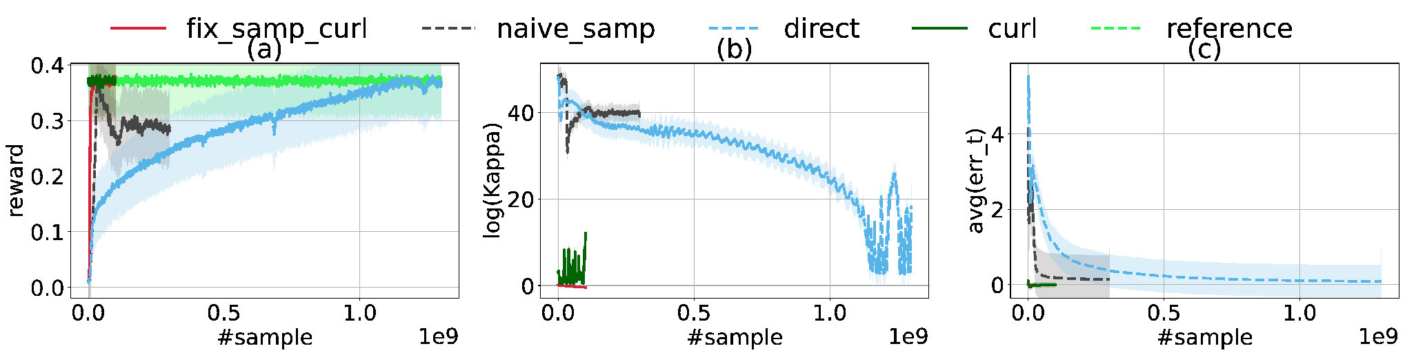
curl, the standard Curriculum Learning, runs Algorithm 2 with pi_t; fix_samp_curl stands for the fixed sampler Curriculum Learning, running Algorithm 2 with pi_s. direct means directly learning in without curriculum, i.e., running Algorithm 1 with None; naive_samp also directly learns in , while using naïve random policy to sample data in Algorithm 1.
6 Performance Analysis
Our analysis contains two important components, namely the sub-optimality gap guarantee of the NPG we proposed, and the efficacy guarantee of Curriculum Learning on BCP. The first component can also be extended to history-dependent policies with features being the tensor products of features from each time step (exponentially large).
6.1 Natural Policy Gradient for Latent MDP
Let denote the true minimizer. We have the following definitions:
Definition 4.
Define for :
(Excess risk) ;
(Transfer error) ;
(Relative condition number) . Note that term inside the expectation is a random quantity as is random.
The expectation is with respect to the randomness in the sequence of weights .
All the quantities are commonly used in literature mentioned in Section 2. is due to that the minimizer from samples may not minimize the population loss . quantifies the approximation error due to feature maps. characterizes the distribution mismatch between and and is a key quantity in Curriculum Learning and will be studied in more details in the following sections.
Our main result is based on a fitting error which depicts the closeness between and any policy .
Definition 5 (Fitting Error).
Suppose the update rule is , define
Theorem 6 shows the convergence rate of Algorithm 1, and its proof is deferred to Section A.3.
Theorem 6.
With Definitions 4, 5 and 9, Algorithm 1 enjoys the following performance bound:
where is the Lyapunov potential function which is only relevant to the initialization.
Remark 4.
①For the results of sample-based NPG with entropy regularization for LMDP, please see Appendix A. ② Taking gives an rate, matching the result in Agarwal et al. 2021. ③ can be reduced using a larger batch size (Lemma 20) that . ④ If some (especially the initialization ) is far away from , may be extremely large (Section 6.2 as an example). If we can find a policy whose is small with a single curriculum, we do not need the multi-step curriculum learning procedure used in Kong et al. 2019.
6.2 Curriculum learning for BCP
For BCP, there exists a threshold policy that is optimal (Beckmann 1990). Suppose the threshold is , then the policy is: accept the -th number if and only if and . For the classical BCP where all the instances have equal probability, the optimal threshold is .
To show that curriculum learning makes the training converge faster, Theorem 6 gives a direct hint: curriculum learning produces a good sampler leading to much smaller than that of a naïve random sampler. Here we focus on the cases where pi_s because the sampler is fixed, while when pi_t it is impossible to analyze a dynamic procedure. We show Theorem 7 to characterize in BCP. Its full statement and proof is deferred to Appendix B.
Theorem 7.
Assume that each number is independent of others and the -th number has a probability of being the maximum so far (Section 4.1). Assume the optimal policy is a -threshold policy and the sampling policy is a -threshold policy. There exists a policy parameterization such that:
| (3) |
where and are of the sampling policy and the naïve random policy, respectively.
To understand how curriculum learning influences , we apply Theorem 7 to three concrete cases. They show that, when the state distribution induced by the optimal policy in the small problem is similar to that in the original large problem, then a single-step curriculum suffices (cf. ④ of Remark 4).
The classical case: an exponential improvement. We study the classical BCP first, where all the permutations are sampled with equal probability. The probability series for this case is . Substituting them into Equation 3 directly gives:
Except for the corner case where , we have that while . Notice that any distribution with leads to an exponential improvement.
A more general case. Now we try to loosen the condition where . Let us consider the case where for (by definition is always equal to ). Equation 3 now becomes:
Clearly, always holds. When is close to , the difference is exponential in .
Failure mode of Curriculum Learning. Lastly we show further relaxing the assumption on leads to failure cases. The extreme case is that all , i.e., the maximum number always comes as the last one. Suppose , then . Hence , larger than . From Equation 3, . Similar as Section 3 of Beckmann 1990, the optimal threshold satisfies:
So letting results in . Further, if and for any , then from Equation 3, . This means that Curriculum Learning can always be manipulated adversarially. Sometimes there is hardly any reasonable curriculum.
Remark 5.
Here we only provide theoretical explanations for BCP when pi_s, because is highly problem-dependent, and the analytical forms for is tractable when the sampler is fixed. For pi_t and other CO problems such as OKD, however, we do not have analytical forms, so we resort to empirical studies (Section 7).
7 Experiments


The experiments’ formulations are modified from Kong et al. 2019. Due to page limit, more formulation details and results are presented in Appendix C, and code can be found at https://github.com/zhourunlong/RL-for-Combinatorial-Optimization. In Curriculum Learning the entire training process splits into at most two phases. We call the training on curriculum (small scale instances) “warm-up phase” and the training on large scale instances “final phase”. If the training is directly on large scale instances, we still call it “final phase” for convenience. For each problem, we run multiple experiments using different distributions of instances. Each experiment contains multiple training methods, e.g., direct training, curriculum learning, etc. To highlight the effect of curriculum learning, we omit the results regarding regularization, and they can be found in supplementary files. All the trainings in the same experiment have the same distributions over LMDPs for final phase and warm-up phase (if any), respectively.
The Best Choice Problem (BCP). We show one of the four experiments in Figure 1. Aside from reward and , we plot the weighted average of according to Theorem 6: avg. All the instance distributions are generated from parameterized series with fixed random seeds, which guarantees reproducibility and comparability. Aside from the fact that the curriculum is a smaller BCP, there is no other explicit relationship between the curriculum and the target environment, so the curriculum can be viewed as random and independent. The experiments clearly demonstrate that curriculum learning can boost the performance by a large margin and curriculum learning indeed dramatically reduces , even the curriculum is randomly generated.
Online Knapsack (decision version, OKD). We show one of the three experiments in Figure 2. and avg() are with respect to the reference policy, a bang-per-buck algorithm, which is not the optimal policy. Thus, they are only for reference. The curriculum generation is also parameterized, random and independent of the target environment. The experiments again demonstrate the effectiveness of curriculum learning and curriculum learning indeed dramatically reduces .
AdWords (decision version, ADW). We show one of the two experiments in Figure 3. The reference policy is obtained by using curriculum learning and training until nearly convergence. The curriculum generation is also parameterized, random and independent of the target environment. The experiments again demonstrate the effectiveness of curriculum learning.
8 Conclusion
We showed online CO problems could be naturally formulated as LMDPs, and we analyzed the convergence rate of NPG for LMDPs. Our theory shows the main benefit of curriculum learning is finding a stronger sampling strategy, especially for classical BCP any curriculum exponentially improves the learning rate. Our empirical results on BCP, OKD, and ADW also corroborated our findings. Our work is the first attempt to systematically study techniques devoted to using RL to tackle online CO problems, which we believe is a fruitful direction worth further investigations.
Acknowledgement
SSD acknowledges the support of NSF IIS 2110170, NSF DMS 2134106, NSF CCF 2212261, NSF IIS 2143493, NSF CCF 2019844, NSF IIS 2229881.
References
- Agarwal et al. (2021) Alekh Agarwal, Sham M. Kakade, J. Lee, and Gaurav Mahajan. On the theory of policy gradient methods: Optimality, approximation, and distribution shift. J. Mach. Learn. Res., 22:98:1–98:76, 2021.
- Albers et al. (2021) Susanne Albers, Arindam Khan, and Leon Ladewig. Improved online algorithms for knapsack and gap in the random order model. Algorithmica, 83:1750 – 1785, 2021.
- Alomrani et al. (2021) Mohammad Ali Alomrani, Reza Moravej, and Elias B Khalil. Deep policies for online bipartite matching: A reinforcement learning approach. arXiv preprint arXiv:2109.10380, 2021.
- Ao et al. (2021) Shuang Ao, Tianyi Zhou, Guodong Long, Qinghua Lu, Liming Zhu, and Jing Jiang. CO-PILOT: COllaborative planning and reinforcement learning on sub-task curriculum. In A. Beygelzimer, Y. Dauphin, P. Liang, and J. Wortman Vaughan (eds.), Advances in Neural Information Processing Systems, 2021. URL https://openreview.net/forum?id=uz_2t6VZby.
- Babaioff et al. (2007) Moshe Babaioff, Nicole Immorlica, David Kempe, and Robert D. Kleinberg. A knapsack secretary problem with applications. In APPROX-RANDOM, 2007.
- Balcan (2020) Maria-Florina Balcan. Data-driven algorithm design. arXiv preprint arXiv:2011.07177, 2020.
- Beckmann (1990) M.J. Beckmann. Dynamic programming and the secretary problem. Computers & Mathematics with Applications, 19(11):25–28, 1990. ISSN 0898-1221. doi: https://doi.org/10.1016/0898-1221(90)90145-A. URL https://www.sciencedirect.com/science/article/pii/089812219090145A.
- Bellmore & Nemhauser (1968) M. Bellmore and G. L. Nemhauser. The traveling salesman problem: A survey. Operations Research, 16(3):538–558, 1968. ISSN 0030364X, 15265463. URL http://www.jstor.org/stable/168581.
- Bello et al. (2017) Irwan Bello, Hieu Pham, Quoc V. Le, Mohammad Norouzi, and Samy Bengio. Neural combinatorial optimization with reinforcement learning, 2017.
- Bengio et al. (2009) Yoshua Bengio, Jérôme Louradour, Ronan Collobert, and Jason Weston. Curriculum learning. In Proceedings of the 26th Annual International Conference on Machine Learning, ICML ’09, pp. 41–48, New York, NY, USA, 2009. Association for Computing Machinery. ISBN 9781605585161. doi: 10.1145/1553374.1553380. URL https://doi.org/10.1145/1553374.1553380.
- Bengio et al. (2020) Yoshua Bengio, Andrea Lodi, and Antoine Prouvost. Machine learning for combinatorial optimization: a methodological tour d’horizon. European Journal of Operational Research, 290, 08 2020. doi: 10.1016/j.ejor.2020.07.063.
- Bhandari & Russo (2021) Jalaj Bhandari and Daniel Russo. On the linear convergence of policy gradient methods for finite mdps. In Arindam Banerjee and Kenji Fukumizu (eds.), Proceedings of The 24th International Conference on Artificial Intelligence and Statistics, volume 130 of Proceedings of Machine Learning Research, pp. 2386–2394. PMLR, 13–15 Apr 2021. URL https://proceedings.mlr.press/v130/bhandari21a.html.
- Brukhim et al. (2021) Nataly Brukhim, Elad Hazan, and Karan Singh. A boosting approach to reinforcement learning, 2021.
- Cappart et al. (2019) Quentin Cappart, Emmanuel Goutierre, David Bergman, and Louis-Martin Rousseau. Improving optimization bounds using machine learning: Decision diagrams meet deep reinforcement learning. Proceedings of the AAAI Conference on Artificial Intelligence, 33(01):1443–1451, Jul. 2019. doi: 10.1609/aaai.v33i01.33011443. URL https://ojs.aaai.org/index.php/AAAI/article/view/3956.
- Cappart et al. (2021) Quentin Cappart, Didier Chételat, Elias B. Khalil, Andrea Lodi, Christopher Morris, and Petar Veličković. Combinatorial optimization and reasoning with graph neural networks. In Zhi-Hua Zhou (ed.), Proceedings of the Thirtieth International Joint Conference on Artificial Intelligence, IJCAI-21, pp. 4348–4355. International Joint Conferences on Artificial Intelligence Organization, 8 2021. doi: 10.24963/ijcai.2021/595. URL https://doi.org/10.24963/ijcai.2021/595. Survey Track.
- Cayci et al. (2021) Semih Cayci, Niao He, and R. Srikant. Linear convergence of entropy-regularized natural policy gradient with linear function approximation, 2021.
- Cen et al. (2021) Shicong Cen, Chen Cheng, Yuxin Chen, Yuting Wei, and Yuejie Chi. Fast global convergence of natural policy gradient methods with entropy regularization. Operations Research, 12 2021. doi: 10.1287/opre.2021.2151.
- Cook (1971) Stephen A. Cook. The complexity of theorem-proving procedures. In Proceedings of the Third Annual ACM Symposium on Theory of Computing, STOC ’71, pp. 151–158, New York, NY, USA, 1971. Association for Computing Machinery. ISBN 9781450374644. doi: 10.1145/800157.805047. URL https://doi.org/10.1145/800157.805047.
- Ding et al. (2021) Yuhao Ding, Junzi Zhang, and Javad Lavaei. On the global convergence of momentum-based policy gradient, 2021.
- Drori et al. (2020) Iddo Drori, Anant Kharkar, William R. Sickinger, Brandon Kates, Qiang Ma, Suwen Ge, Eden Dolev, Brenda L Dietrich, David P. Williamson, and Madeleine Udell. Learning to solve combinatorial optimization problems on real-world graphs in linear time. 2020 19th IEEE International Conference on Machine Learning and Applications (ICMLA), pp. 19–24, 2020.
- Flood (1956) Merrill M. Flood. The traveling-salesman problem. Operations Research, 4(1):61–75, 1956. ISSN 0030364X, 15265463. URL http://www.jstor.org/stable/167517.
- Garg et al. (2008) Naveen Garg, Anupam Gupta, Stefano Leonardi, and Piotr Sankowski. Stochastic analyses for online combinatorial optimization problems. 2008.
- Goemans & Williamson (1995) Michel X. Goemans and David P. Williamson. Improved approximation algorithms for maximum cut and satisfiability problems using semidefinite programming. J. ACM, 42(6):1115–1145, nov 1995. ISSN 0004-5411. doi: 10.1145/227683.227684. URL https://doi.org/10.1145/227683.227684.
- Graves et al. (2017) Alex Graves, Marc G. Bellemare, Jacob Menick, Rémi Munos, and Koray Kavukcuoglu. Automated curriculum learning for neural networks. In Doina Precup and Yee Whye Teh (eds.), Proceedings of the 34th International Conference on Machine Learning, volume 70 of Proceedings of Machine Learning Research, pp. 1311–1320. PMLR, 06–11 Aug 2017. URL https://proceedings.mlr.press/v70/graves17a.html.
- Grötschel et al. (2001) Martin Grötschel, Sven O Krumke, Jörg Rambau, Thomas Winter, and Uwe T Zimmermann. Combinatorial online optimization in real time. Online optimization of large scale systems, pp. 679–704, 2001.
- Huang (2019) Zhiyi Huang. Online combinatorial optimization problems with non-linear objectives. In Nonlinear Combinatorial Optimization, pp. 179–205. Springer, 2019.
- Huang et al. (2019) Zhiyi Huang, Peng Binghui, Zhihao Tang, Runzhou Tao, Xiaowei Wu, and Yuhao Zhang. Tight Competitive Ratios of Classic Matching Algorithms in the Fully Online Model, pp. 2875–2886. 01 2019. ISBN 978-1-61197-548-2. doi: 10.1137/1.9781611975482.178.
- Kakade (2002) Sham M Kakade. A natural policy gradient. In T. Dietterich, S. Becker, and Z. Ghahramani (eds.), Advances in Neural Information Processing Systems, volume 14. MIT Press, 2002. URL https://proceedings.neurips.cc/paper/2001/file/4b86abe48d358ecf194c56c69108433e-Paper.pdf.
- Karp (1972) Richard Karp. Reducibility among combinatorial problems. volume 40, pp. 85–103, 01 1972. ISBN 978-3-540-68274-5. doi: 10.1007/978-3-540-68279-0_8.
- Khalil et al. (2017) Elias Boutros Khalil, Hanjun Dai, Yuyu Zhang, Bistra N. Dilkina, and Le Song. Learning combinatorial optimization algorithms over graphs. In NIPS, 2017.
- Kong et al. (2019) Weiwei Kong, Christopher Liaw, Aranyak Mehta, and D. Sivakumar. A new dog learns old tricks: Rl finds classic optimization algorithms. In ICLR, 2019.
- Kool et al. (2019) Wouter Kool, Herke van Hoof, and Max Welling. Attention, learn to solve routing problems! In ICLR, 2019.
- Kwon et al. (2021a) Jeongyeol Kwon, Yonathan Efroni, Constantine Caramanis, and Shie Mannor. Rl for latent mdps: Regret guarantees and a lower bound. In M. Ranzato, A. Beygelzimer, Y. Dauphin, P.S. Liang, and J. Wortman Vaughan (eds.), Advances in Neural Information Processing Systems, volume 34, pp. 24523–24534. Curran Associates, Inc., 2021a. URL https://proceedings.neurips.cc/paper/2021/file/cd755a6c6b699f3262bcc2aa46ab507e-Paper.pdf.
- Kwon et al. (2021b) Jeongyeol Kwon, Yonathan Efroni, Constantine Caramanis, and Shie Mannor. Reinforcement learning in reward-mixing mdps. In NeurIPS, 2021b.
- Liu et al. (2020) Yanli Liu, Kaiqing Zhang, Tamer Basar, and Wotao Yin. An improved analysis of (variance-reduced) policy gradient and natural policy gradient methods. In H. Larochelle, M. Ranzato, R. Hadsell, M. F. Balcan, and H. Lin (eds.), Advances in Neural Information Processing Systems, volume 33, pp. 7624–7636. Curran Associates, Inc., 2020. URL https://proceedings.neurips.cc/paper/2020/file/56577889b3c1cd083b6d7b32d32f99d5-Paper.pdf.
- Mazyavkina et al. (2021) Nina Mazyavkina, Sergey Sviridov, Sergei Ivanov, and Evgeny Burnaev. Reinforcement learning for combinatorial optimization: A survey. Computers & Operations Research, 134:105400, 05 2021. doi: 10.1016/j.cor.2021.105400.
- Mehta et al. (2007) Aranyak Mehta, Amin Saberi, Umesh Vazirani, and Vijay Vazirani. Adwords and generalized online matching. Journal of the ACM (JACM), 54(5):22–es, 2007.
- Mei et al. (2020) Jincheng Mei, Chenjun Xiao, Csaba Szepesvari, and Dale Schuurmans. On the global convergence rates of softmax policy gradient methods. In Hal Daumé III and Aarti Singh (eds.), Proceedings of the 37th International Conference on Machine Learning, volume 119 of Proceedings of Machine Learning Research, pp. 6820–6829. PMLR, 13–18 Jul 2020. URL http://proceedings.mlr.press/v119/mei20b.html.
- Mirhoseini et al. (2021) Azalia Mirhoseini, Anna Goldie, Mustafa Yazgan, Joe Wenjie Jiang, Ebrahim M. Songhori, Shen Wang, Young-Joon Lee, Eric Johnson, Omkar Pathak, Azade Nazi, Jiwoo Pak, Andy Tong, Kavya Srinivasa, Will Hang, Emre Tuncer, Quoc V. Le, James Laudon, Richard Ho, Roger Carpenter, and Jeff Dean. A graph placement methodology for fast chip design. Nature, 594 7862:207–212, 2021.
- Narvekar et al. (2020) Sanmit Narvekar, Bei Peng, Matteo Leonetti, Jivko Sinapov, Matthew E. Taylor, and Peter Stone. Curriculum learning for reinforcement learning domains: A framework and survey. J. Mach. Learn. Res., 21:181:1–181:50, 2020.
- Nazari et al. (2018) M. Nazari, Afshin Oroojlooy, Lawrence V. Snyder, and Martin Takác. Reinforcement learning for solving the vehicle routing problem. In NeurIPS, 2018.
- Oren et al. (2021) Joel Oren, Chana Ross, Maksym Lefarov, Felix Richter, Ayal Taitler, Zohar Feldman, Christian Daniel, and Dotan Di Castro. Solo: Search online, learn offline for combinatorial optimization problems. ArXiv, abs/2104.01646, 2021.
- Pérez-Dattari et al. (2018) Rodrigo Pérez-Dattari, Carlos Celemin, Javier Ruiz del Solar, and Jens Kober. Interactive learning with corrective feedback for policies based on deep neural networks. In ISER, 2018.
- Scholten et al. (2019) Jan Scholten, Daan Wout, Carlos Celemin, and Jens Kober. Deep reinforcement learning with feedback-based exploration. 2019 IEEE 58th Conference on Decision and Control (CDC), Dec 2019. doi: 10.1109/cdc40024.2019.9029503. URL http://dx.doi.org/10.1109/CDC40024.2019.9029503.
- Selsam et al. (2019) Daniel Selsam, Matthew Lamm, Benedikt Bünz, Percy Liang, Leonardo de Moura, and David L. Dill. Learning a SAT solver from single-bit supervision. In International Conference on Learning Representations, 2019. URL https://openreview.net/forum?id=HJMC_iA5tm.
- Steimle et al. (2021) Lauren N. Steimle, David L. Kaufman, and Brian T. Denton. Multi-model markov decision processes. IISE Transactions, 53(10):1124–1139, 2021. doi: 10.1080/24725854.2021.1895454. URL https://doi.org/10.1080/24725854.2021.1895454.
- Trakhtenbrot (1984) B.A. Trakhtenbrot. A survey of russian approaches to perebor (brute-force searches) algorithms. Annals of the History of Computing, 6(4):384–400, 1984. doi: 10.1109/MAHC.1984.10036.
- Vesselinova et al. (2020) Natalia Vesselinova, Rebecca Steinert, Daniel F. Perez-Ramirez, and Magnus Boman. Learning combinatorial optimization on graphs: A survey with applications to networking. IEEE Access, 8:120388–120416, 2020.
- Wang et al. (2020) Lingxiao Wang, Qi Cai, Zhuoran Yang, and Zhaoran Wang. Neural policy gradient methods: Global optimality and rates of convergence. In International Conference on Learning Representations, 2020. URL https://openreview.net/forum?id=BJgQfkSYDS.
- Willems et al. (2020) Lucas Willems, Salem Lahlou, and Yoshua Bengio. Mastering rate based curriculum learning, 2020.
- Zhang et al. (2021) Junzi Zhang, Jongho Kim, Brendan O’Donoghue, and Stephen Boyd. Sample efficient reinforcement learning with reinforce. In AAAI, 2021.
- Zhou et al. (2020a) Tianyi Zhou, Shengjie Wang, and Jeffrey Bilmes. Curriculum learning by dynamic instance hardness. In H. Larochelle, M. Ranzato, R. Hadsell, M. F. Balcan, and H. Lin (eds.), Advances in Neural Information Processing Systems, volume 33, pp. 8602–8613. Curran Associates, Inc., 2020a. URL https://proceedings.neurips.cc/paper/2020/file/62000dee5a05a6a71de3a6127a68778a-Paper.pdf.
- Zhou et al. (2021a) Tianyi Zhou, Shengjie Wang, and Jeff Bilmes. Curriculum learning by optimizing learning dynamics. In Arindam Banerjee and Kenji Fukumizu (eds.), Proceedings of The 24th International Conference on Artificial Intelligence and Statistics, volume 130 of Proceedings of Machine Learning Research, pp. 433–441. PMLR, 13–15 Apr 2021a. URL https://proceedings.mlr.press/v130/zhou21a.html.
- Zhou et al. (2021b) Tianyi Zhou, Shengjie Wang, and Jeff Bilmes. Robust curriculum learning: from clean label detection to noisy label self-correction. In International Conference on Learning Representations, 2021b. URL https://openreview.net/forum?id=lmTWnm3coJJ.
- Zhou et al. (2020b) Yanqi Zhou, Sudip Roy, Amirali Abdolrashidi, Daniel Wong, Peter Ma, Qiumin Xu, Hanxiao Liu, Phitchaya Phothilimtha, Shen Wang, Anna Goldie, Azalia Mirhoseini, and James Laudon. Transferable graph optimizers for ml compilers. In H. Larochelle, M. Ranzato, R. Hadsell, M.F. Balcan, and H. Lin (eds.), Advances in Neural Information Processing Systems, volume 33, pp. 13844–13855. Curran Associates, Inc., 2020b. URL https://proceedings.neurips.cc/paper/2020/file/9f29450d2eb58feb555078bdefe28aa5-Paper.pdf.
Appendix A Full Results of the Main Algorithm and Theorem for Entropy Regularization
A.1 Notations and Definitions
Entropy regularized value function, Q-function and advantage function.
We incorporate entropy regularization for completeness because prior works (especially empirical works) used it to facilitate training. We define the value function in a unified way: is defined as the sum of future -regularized rewards starting from and executing for steps in , i.e.,
where , and the expectation is with respect to the randomness of trajectory induced by in . Clearly, .
For any , with we define
In fact, .
Denote then . The original goal is to find . Under regularization, we seek for instead. Denote . Since , the regularized optimal policy can be nearly optimal as long as the regularization coefficient is small enough. For notational ease, we abuse with .
The Q-function can be defined in a similar manner:
and the advantage function is defined as .
Denote and for convenience.
Definition 8 (Definition 2 with entropy regularization).
Let be the parameter update weight, then NPG is related to finding the minimizer for the following function:
Definition 9 (Lyapunov Potential Function (Cayci et al. 2021)).
We define the potential function as follows: for any ,
A.2 Algorithms
Algorithm 3 is the full version of Algorithm 1, with support of entropy regularization. Algorithm 4 is the skipped sampling function.
A.3 Performance of Natural Policy Gradient for LMDP
We restate Theorem 6 with entropy regularization.
Theorem 6 (Full Statement of Theorem 6).
With Definitions 4, 5 and 9, Algorithm 3 enjoys the following performance bound:
Proof.
Here we make shorthands for the sub-optimality gap and potential function: and . From Lemma 16 we have
Taking expectation over the update weights, we have
Thus,
where the last step uses the fact that . This is a weighted average, so by normalizing the coefficients,
where the last step comes from Lemma 17 and Jensen’s inequality. This completes the proof. ∎
Aside from Remark 4, we have extra remarks:
Remark 6.
①This is the first result for LMDP and sample-based NPG with entropy regularization. ② For any fixed we have a linear convergence, which matches the result of discounted infinite horizon MDP (Theorem 1 in Cayci et al. 2021); the limit when tends to is (which implies an rate), matching the result in Agarwal et al. 2021.
Appendix B Results of Curriculum Learning for the Best Choice Problem (BCP)
Theorem 7 (Formal statement of Theorem 7).
For BCP, set pi_s in Algorithm 2. Assume that each number is independent from others and the -th number has probability of being the best so far (see formulation in Section 4.1 and Section C.1). Assume the optimal policy is a -threshold policy and the sampling policy is a -threshold policy. There exists a policy parameterization and quantities
such that and . Here and correspond to induced by the -threshold policy and the naïve random policy respectively.
Proof.
We need to calculate three state-action visitation distributions: that induced by the optimal policy, ; that induced by the sampler which is the optimal for the curriculum, ; and that induced by the naïve random sampler, . This then boils down to calculating the state(-action) visitation distribution under two types of policies: any threshold policy and the naïve random policy.
For any policy , denote as the probability for the agent acting under to see states with arbitrary . We do not need to take the terminal state into consideration, since it stays in a zero-reward loop and contributes to . We use the LMDP distribution parameterization described in Section 7.
Denote as the -threshold policy, i.e. accept if and only if and . Then
Denote as the naïve random policy, i.e., accept any number with probability regardless of the state. Then
For any , we can see that the state visitation distribution satisfies and .
To show the possible largest difference, we use a parameterization that for each state , One-hot. The policy is then satisfied into
because there are only two actions. Denote , we have
Now suppose the optimal threshold and the threshold learned through curriculum are and , then
Denote . From parameterization we know all are orthogonal. Abusing with , we have
We can separately consider each because of the orthogonal features. Observe that , so for , its corresponding term in is maximized when and is equal to . By definition, . Since , we have where and the corresponding term is . So
We now have an order-accurate result for . Direct computation gives
This completes the proof. ∎
Appendix C Full Experiments
Here are all the experiments not shown in Section 7. All the experiments were run on a server with CPU AMD Ryzen 9 3950X, GPU NVIDIA GeForce 2080 Super and 128G memory. For legend description please refer to the caption of Figure 1. For code please refer to https://github.com/zhourunlong/RL-for-Combinatorial-Optimization.
Policy parameterization.
- •
For BCP and OKD, there are exactly two actions, so we can use instead of and . Now the policy is and
- •
For ADW, there are actions ( for assigning a slot to advertisers and for not assigning it). So, we must follow the canonical form of log-linear policies.
Training schemes.
We ran nine experiments in total, four for BCP, three for OKD, and two for ADW. The difference between the experiments of the same problem lies in the distribution over instances (i.e., ). In the following subsections, we will introduce how we parameterized the distribution in detail. In a single experiment, we ran eight setups, each representing a combination of sampler policies, initialization policies of the final phase, and whether we used regularization. For visual clarity, we did not plot setups with entropy regularization, but the readers can plot it using plot.py in the supplementary files. We make a detailed list of the training schemes in Table 1.
| Abbreviation | Detailed setup | Script |
| fix_samp_curl | Fixed sampler curriculum learning. In the warm-up phase, train a policy from scratch (with zero initialization in parameters) using a small environment . In the final phase, change to the true environment , use as the sampler policy to train a policy from scratch. | Run Alg. 2 with and . |
| fix_samp_curl_reg | The same as fix_samp_curl, but add entropy regularization to both phases. | Run Alg. 2 with and . |
| direct | Direct learning. Only the final phase. Train a policy from scratch directly in . | Run Alg. 1 with , None and . |
| direct_reg | The same as direct, but add entropy regularization. | Run Alg. 1 with , None and . |
| naive_samp | Learning with the naïve sampler. Only the final phase. Use the naïve random policy as the sampler to train a policy from scratch in . | Run Alg. 1 with , naïve random policy and . |
| naive_samp_reg | The same as naive_samp, but add entropy regularization. | Run Alg. 1 with , naive random policy and . |
| curl | Curriculum learning. In the warm-up phase, train a policy from scratch in . In the final phase, change to and continue on training . | Run Alg. 2 with and . |
| curl_reg | The same as curl, but add entropy regularization. | Run Alg. 2 with and . |
| reference | This is the reference policy. For BCP, it is exactly the optimal policy since it can be calculated. For OKD, it is a bang-per-buck policy and is not the optimal policy (whose exact form is not clear). For ADW, it is the near optimal policy in our restricted policy / feature class (trained using curriculum learning). | N/A |
C.1 The Best Choice Problem (BCP)
State and action spaces.
States with are the same. To make the problem “scale-invariant”, we use to represent . So the states are . There is an additional terminal state . For each state, the agent can either accept or reject.
Transition and reward.
Any action in leads back to . Once the agent accepts the -th number, the state transits into , and reward is if is the maximum in the instance. If the agent rejects, then the state goes to if and if . For all other cases, rewards are .
Feature mapping.
Recall that all states are of the form where . We set a degree and the feature mapping is constructed as the collection of polynomial bases with degree less than ():
LMDP distribution.
We model the distribution as follows: for each , we can have with probability and is independent from other . By definition, while other can be arbitrary. The classical BCP satisfies . We also experimented on three other distributions (so in total there are four experiments), each with a series of numbers and set .
For each experiment, we run eight setups, each with different combinations of sampler policies, initialization policies of the final phase, and the value of regularization coefficient . For the warm-up phases we set and for final phases .
Results.
Figure 4 (with its full view Figure 5), Figure 6, Figure 7, along with Figure 1 (with seed 2018011309) show four experiments of BCP. They shared a learning rate of , batch size of per step in horizon, final and warm-up (if applied curriculum learning). 33 3 All the four trainings shown in the figures have their counterparts with regularization (). Check the supplementary files and use TensorBoard for visualization.
The experiment in Figure 4 was done in the classical BCP environment, i.e., all permutations have probability to be sampled. Experiments Figure 1, Figure 6 and Figure 7 were done with other distributions: the only differences are the random seeds, which we fixed and used to generate s for reproducibility.
The experiment of classical BCP was run until the direct training of converges, while all other experiments were run to a maximum episode of (hence sample number of ).
The optimal policy was derived from dynamic programming.



C.2 Online Knapsack (decision version, OKD)
State and action spaces.
The states are represented as
where for (in the instance). There is an additional terminal state . For each state (including for simplicity), the agent can either accept or reject.
Transition and reward.
The transition is implied by the definition of the problem. Any action in terminal state leads back to . The item is successfully chosen if and only if the agent accepts and the budget is sufficient. A reward of is given only the first time , and then the state goes to . For all other cases, reward is .
Feature mapping.
Suppose the state is . We set a degree and the feature mapping is constructed as the collection of polynomial bases with degree less than (): where .
LMDP distribution.
In Section 3.2 the values and sizes are sampled from and . If or is not , we model the distribution as: first set a granularity and take numbers . represents the (unnormalized) probability that . To sample, we take Multinomial and return .
For each experiment, we ran four setups, each with different combinations of sampler policies and initialization policies of the final phase. For the warm-up phases and for final phases we set in all experiments, while and vary. In one experiment it satisfies that are close for warm-up and final, and increases from warm-up to final.
Results.
Figure 8, Figure 9, along with Figure 2 (with ) show three experiments of OKD. They shared a learning rate of , batch size of per step in horizon, final and warm-up (if applied curriculum learning).
Experiments in Figure 8 and Figure 9 were done with other value and size distributions: the only differences are the random seeds, which we fixed and used to generate and for reproducibility.
All experiments were run to a maximum episode of (hence sample number of ).
The reference policy is a bang-per-buck algorithm (Section 3.1 of Kong et al. 2019): given a threshold , accept -th item if . We searched for the optimal with respect to Online Knapsack because we found that in general the reward is unimodal to and contains no “plain area”, so we can easily apply ternary search (the reward of OKD contains “plain area”).


C.3 AdWords (decision version, ADW)
State and action spaces.
The states are represented as
where is equal to the total revenue up until now. There is an additional terminal state . For each state (including for simplicity), the agent has actions, with representing not assigning the slot and representing assigning to the corresponding advertiser.
Transition and reward.
The transition is implied by the definition of the problem. Any action in terminal state leads back to . The slot is successfully assigned to advertiser if and only if the action is and . The next state is then with and . A reward of is given only the first time , and then the state goes to . For all other cases, reward is .
Feature mapping.
The feature design in ADW is a bit tricky, since the state dimension is super large. We simplify the setting by assuming all the advertisers are symmetric, so we design a function and for action ,
and
Actually, not assigning the slot is equal to assigning the slot to a virtual advertiser with value .
We set a degree and is constructed as the collection of polynomial bases with degree less than (): where .
LMDP distribution.
In Section 3.3 the values are sampled from . If is not , we model the distribution in the same manner as in OKD. For each experiment, we ran four setups, each with different combinations of sampler policies and initialization policies of the final phase.
In the experiment depicted in Figure 3: For the warm-up phases we set and . For final phases we set and . The distributions are parameterized random ones with .
In the experiment depicted in Figure 10: For the warm-up phases we set and . For final phases we set and . The distributions are specially designed distributions, with probability it has a value, and the rest mass is random on . This distribution type has a special near optimal policy class: either pick two , or pick anything in .
Results.
Figure 3 and Figure 10 are experiments of ADW. They shared a learning rate of and batch size of per step in horizon.
The reference policy is obtained by first running a curriculum learning, then using the learned policy as the reference policy. This is because after we simplify the feature representation, we need to compare with the near optimal policy inside this restricted policy / feature class.

Appendix D Technical Details and Lemmas
D.1 Natural Policy Gradient for LMDP
This section is a complement to Section 5. We give details about the correctness of Natural Policy Gradient for LMDP.
Theorem 12 is the finite-horizon Policy Gradient Theorem for LMDP, which takes the mixing weight into consideration.
According to Agarwal et al. 2021, the unconstrained, full-information NPG update weight satisfies . Lemma 13 and Lemma 14 together show that: it is equivalent to finding a minimizer of the fitting compatible function approximation loss (Definition 8).
Theorem 12 (Policy Gradient Theorem for LMDP).
For any policy parameterized by , and any ,
As a result,
Proof.
For any and , since , we have
Hence
Next we focus on the second term. From the Bellman equation,
Particularly, . So
where we used the definition of and . So by rearranging the terms, we complete the proof. ∎
Lemma 13.
Suppose where and , then is a solution to the equation .
Proof.
Denote , then the equation is reduced to . Suppose the singular value decomposition of is where where and are unitary, and singular values are . So and . Notice that
we can then derive the pseudo-inverse of this particular diagonal matrix as
It is then easy to verify that . Finally,
This completes the proof. ∎
Lemma 14 (NPG Update Rule).
The update rule where
is equivalent to , where is a minimizer of the function
Proof.
Suppose is any minimizer of , we have , hence
Since , then
Now we assign as indices to all , and set
where is the index assigned to . Then and where
We now conclude the proof by utilizing Lemma 13. ∎
D.2 Auxiliary lemmas used in the main results
Lemma 15 (Performance Difference Lemma).
For any two policies and , and any ,
As a result,
Proof.
First we fix . By definition of the value function, we have
where the last step uses law of iterated expectations. Since
we have
By taking expectation over , we have
The proof is completed by reversing the order of . ∎
Lemma 16 (Lyapunov Drift).
Recall definitions in Definitions 9 and 5. We have that:
Proof.
Denote . This proof follows a similar manner as in that of Lemma 6 in Cayci et al. 2021. By smoothness (see Remark 6.7 in Agarwal et al. 2021),
By the definition of ,
By the definition of , Lemma 15 and again the definition of , we finally have
which completes the proof. ∎
Lemma 17.
Recall that is the true minimizer of in domain . defined in Definition 5 satisfies
Proof.
The proof is similar to that of Theorem 6.1 in Agarwal et al. 2021. We make the following decomposition of :
Since , normalize the coefficients and apply Jensen’s inequality, then
| ① | |||
Similarly,
| ② | |||
where in (i), for vector , denote for a symmetric positive semi-definite matrix . Due to that minimizes over the set , the first-order optimality condition implies that
for any . Therefore,
So finally we have
This completes the proof. ∎
D.3 Bounding
Lemma 18 (Hoeffding’s Inequality).
Suppose are i.i.d. random variables taking values in , with expectation . Let denote their average, then for any ,
Lemma 19.
For any policy , any state and any ,
Proof.
The first inequality is straightforward, so we focus on the second part. Set and , then
where the penultimate step comes from concavity of and Jensen’s inequality. Let , then . Recall that , so increases when and decreases when . Since we complete the proof. ∎
Lemma 20 (Loss Function Concentration).
If set None and , then with probability , the update weight sequence of Algorithm 3 satisfies: for any ,
where
If None and , then with probability , the update weight sequence of Algorithm 3 satisfies: for any ,
where
Proof.
We first prove the None case. For time step , Algorithm 3 samples trajectories. Abusing the notation, denote
Notice that ① is a constant. From Algorithm 3, is the minimizer of ② (hence ) inside the ball . From , we know that . So . From Algorithm 4, we know that any sampled satisfies . So . We first have that
| (4) |
To apply any standard concentration inequality, we next need to calculate the expectation of ②. According to Monte Carlo sampling and Lemma 19, for any and , we have
Denote as the exact policy gradient at time step , then
Since Monte Carlo sampling correctly estimates state-action visitation distribution, . Notice that is linear in entries of , we have . Now we are in the position to show that
After applying union bound for all , with probability the following holds for any :
Hence
For None and , we notice that and hence . Moreover, . So by slightly modifying the proof we can get the result. ∎