Many-body Green’s function approaches to the doped Fröhlich solid:
Exact solutions and anomalous mass enhancement
Abstract
In polar semiconductors and insulators, the Fröhlich interaction between electrons and long-wavelength longitudinal optical phonons induces a many-body renormalization of the carrier effective masses and the appearence of characteristic phonon sidebands in the spectral function, commonly dubbed ‘polaron satellites’. The simplest model that captures these effects is the Fröhlich model, whereby electrons in a parabolic band interact with a dispersionless longitudinal optical phonon. The Fröhlich model has been employed in a number of seminal papers, from early perturbation-theory approaches to modern diagrammatic Monte Carlo calculations. One limitation of this model is that it focuses on undoped systems, thus ignoring carrier screening and Pauli blocking effects that are present in real experiments on doped samples. To overcome this limitation, we here extend the Fröhlich model to the case of doped systems, and we provide exact solutions for the electron spectral function, mass enhancement, and polaron satellites. We perform the analysis using two approaches, namely Dyson’s equation with the Fan-Migdal self-energy, and the second-order cumulant expansion. We find that these two approaches provide qualitatively different results. In particular, the Dyson’s approach yields better quasiparticle masses and worse satellites, while the cumulant approach provides better satellite structures, at the price of worse quasiparticle masses. Both approaches yield an anomalous enhancement of the electron effective mass at finite doping levels, which in turn leads to a breakdown of the quasiparticle picture in a significant portion of the phase diagram.
I Introduction
The Fröhlich interaction, that is the coupling between electrons and long-wavelength longitudinal optical (LO) phonons in polar semiconductors and insulators, constitutes one of the earliest and most intensely studied manifestations of electron-phonon physics.Fröhlich et al. 1950; Devreese; Devreese and Alexandrov 2009 On the theory side, Fröhlich couplings have received considerable attention during the past few years, as efficient ab initio techniques to describe these processes have become available.Verdi and Giustino 2015; Sjakste et al. 2015; Park et al. 2020; Brunin et al. 2020 Meanwhile, a recent report has demonstrated the remarkable effectiveness of a generalized Fröhlich model in the prediction of zero-point band-gap renormalization when compared to highly accurate ab-initio calculations.Miglio et al. 2020 On the experiment side, the Fröhlich interaction has long been known to play an important role in the carrier transport properties of doped semiconductors and oxides Ohtomo and Hwang 2004; Herranz et al. 2007 and in their superconducting phases.Schooley et al. 1964; Schooley et al. 1965; Lin et al. 2014 More recently, Fröhlich couplings have been identified as the origin of intriguing phonon sidebands in the photoelectron spectra of many compounds, including SrTiO3 (STO),Meevasana et al. 2011; Santander-Syro et al. 2011; Chen et al. 2015; Wang et al. 2016 TiO2,Moser et al. 2013, EuO,Riley et al. 2018 CaMnO3,Husanu et al. 2020 and ZnO.Yukawa et al. 2016 In turn, these sidebands have been linked to the observation of superconducting phases in bulk and interfacial systems.Lee et al. 2014; Lin et al. 2014; Cancellieri et al. 2016
The most direct route to investigate the effect of Fröhlich couplings on electron band structures is via angle-resolved photoelectron spectroscopy (ARPES). In ARPES experiments, electrons are extracted from a sample via laser or synchrotron light, and the energy and momentum of the electron prior to exiting the sample can be reconstructed by an analyzer. This setup provides a direct image of the momentum-resolved electron spectral function, i.e. the many-body electron band structure. Since only occupied electronic states can be probed by ARPES, it is necessary to dope electrons into the sample in order to image the band edges. These electrons interact with all phonons in the sample; however, in polar semiconductors and oxides the dominant coupling mechanism is the Fröhlich interaction with long-wavelength LO phonons, because the associated coupling matrix element diverges at long wavelength.Giustino 2017 This coupling enhances the carrier effective mass and leads to the appearence of phonon sidebands below the conduction band edge, usually called ‘polaron satellites’.Moser et al. 2013; Wang et al. 2016; Lee et al. 2014; Cancellieri et al. 2016 A schematic illustration of these effects is shown in Fig. 1.
The description of these low-energy structures using ab initio many-body methods is challenging.Story et al. 2014 In the case of standard metals, where the Fermi energy is much larger than the characteristic phonon energy , , Migdal’s theorem guarantees that the interaction is well described by non-crossing electron-phonon self-energy diagrams.Migdal 1958; Mahan 1993; Giustino 2017 However, degenerate semiconductors including doped oxides typically possess a Fermi energy comparable to the characteristic phonon energy, .Bretz-Sullivan et al. This scenario falls outside of the validity limit of the Migdal approximation. As a result, calculations on these systems based on the Migdal approximation suffer from well-documented shortcomings, for example incorrect energetics of the satellite structures shown in Fig. 1.Story et al. 2014; Verdi et al. 2017; Nery et al. 2018; Zhou and Bernardi 2019
One promising strategy to overcome this limitation is provided by the cumulant expansion method.Langreth 1970; Hedin 1980; Aryasetiawan et al. 1996 In its original formulation, this approach was introduced to study the coupling of core holes to plasma excitations in metals.Langreth 1970 The generalization of this approach to valence electrons Hedin 1980 enabled the first ab initio calculations of plasmon satellites in elemental metals.Aryasetiawan et al. 1996 More recently, the cumulant approach has been employed to improve the description of spectral satellites arising from electron-plasmon interactions in GW calculations.Lischner et al. 2013; Kas et al. 2014; Caruso and Giustino 2015; Caruso et al. 2015; Caruso and Giustino 2016a; Caruso and Giustino 2016b; Gumhalter et al. 2016; Zhou et al. 2018; Tzavala et al. 2020 In the context of electron-phonon physics, the cumulant expansion has successfully been employed to calculate phonon sidebands in systems exhibiting Fröhlich coupling.Story et al. 2014; Verdi et al. 2017; Caruso et al. 2018; Riley et al. 2018; Nery et al. 2018; Zhou and Bernardi 2019; Antonius et al. 2020; Zhou et al. 2020
Despite much progress on the front of ab initio calculations, we still lack a simple analytical model that captures the essential features of Fröhlich interactions in doped systems, and that can be used as a reference benchmark for validating ab initio implementations. This gap is particularly critical as ab initio calculations of Fröhlich couplings require extremely dense Brillouin zone grids, and are therefore computationally very demanding. As a result, it is difficult to systematically explore the parameter space and extract general trends.
The most popular model employed to investigate electronic couplings to polar LO phonons is the Fröhlich model.Fröhlich et al. 1950 This model consists of an electron in a parabolic electron band coupled to a dispersionless LO phonon.Fröhlich et al. 1950; Lee and Pines 1952; Röseler 1968; Smondyrev 1986; Selyugin and Smondyrev 1989; Feynman 1955 It forms the basis for a number of seminal papers on electron-phonon interactions and polarons,Devreese; Devreese and Alexandrov 2009; Mahan 1993 and is routinely used for testing advanced many-body techniques such as the diagrammatic Monte Carlo method.Prokof’ev and Svistunov 1998; Mishchenko et al. 2000 However, this model describes a single electron coupled to a phonon bath, therefore it does not include the effects of band filling (shown schematically in Fig. 1), and the associated screening of the polar interaction by free carriers. Without including free carriers, the Fröhlich model cannot reproduce the correct energetic ordering of bands and satellites as shown in Fig. 1 and observed in experiments; instead, the Fröhlich model incorrectly yields satellites above the conduction band bottom.Mishchenko et al. 2000; Nery et al. 2018
In this work, we go beyond the original Fröhlich model by deriving analytic expressions for the electron self-energy and spectral function for electron-LO phonon interactions in the presence of free carriers. This model constitutes an idealization of Fröhlich interactions in many degenerate semiconductors and doped oxides that have been investigated via photoelectron spectroscopy.Chen et al. 2015; Wang et al. 2016; Moser et al. 2013; Riley et al. 2018; Husanu et al. 2020; Yukawa et al. 2016; Lee et al. 2014; Lin et al. 2014; Cancellieri et al. 2016 We refer to this extended model as the “doped Fröhlich solid”. For this model, we derive the Fan-Migdal self-energy, and use it to obtain the electron spectral function within both Dyson’s equation and the second-order cumulant expansion method. For each approach, we analyze the quasiparticle (QP) band structure, the phonon satellites, and the mass enhancement, and we identify advantages and shortcomings. In particular, we show that both approaches yield anomalous electron mass enhancements at finite Fermi levels. This enhancement is so strong that the band curvature is inverted in a large region of the phase diagram, leading to a breakdown of the QP picture. This failure is more pronounced in the cumulant approach.
This manuscript is organized as follows: In Sec. II, we formally introduce the doped Fröhlich solid, the Fan-Migdal self-energy, and how to obtain the spectral function within either Dyson’s method or the second-order cumulant expansion. In Sec. III.1, we review the classic Fröhlich polaron problem as the empty-band limit of the doped Fröhlich solid. We show that the empty-band model fails to reproduce the correct energetic ordering of bands and satellites that is observed in experiments. This shortcoming is remedied in Sec. III.2, where we introduce free carriers and a finite Fermi level in the model. In this case we only consider band filling effects, without taking into account the screening of the Fröhlich interaction by the free carriers. This scenario is relevant for experiments in the anti-adabatic regime (). In Sec. III.3, we include both the effect of band filling and free-carrier screening, and derive semi-analytical self-energy and spectral functions. This more accurate model is found to capture most of the features observed in ARPES experiments in doped oxides. For easier orientation within this manuscript, we reference all equations for the QP energy and effective mass for the three considered scenarios in table 1. Section IV connects our Dyson and cumulant spectra to experimental data by comparing calculated and measured quasi-particle weights. In Sec. V we summarize our results and discuss the implications of our findings for ab initio calculations of Fröhlich couplings. Lastly, we report details of the derivations in the appendices.
II Model setup and general expressions for the self-energy and the spectral function
II.1 The doped Fröhlich solid
The Fröhlich Hamiltonian for electrons coupled to dispersionless LO phonons is given by:Giustino 2017
| (1) |
where , , , and are electron wavevectors, phonon wavevectors, fermion annihilation operators, and boson annihilation operators, respectively. The single-particle energies of the electrons are indicated by , is the LO phonon energy, with is the Fröhlich matrix element, and is the number of unit cells in the Born-von-Kármán supercell.
In this model, the electron-electron interation is assumed to be already taken into account by the effective mass , and the electron band structure is simply given by , with . Throughout this manuscript we consider the system at zero temperature, so that the electron occupations are described by the Heaviside function , where is the Fermi wavevector.
The matrix element of the Fröhlich interaction is given by:Verdi and Giustino 2015; Sjakste et al. 2015
| (2) |
where is the volume of the crystal cell consisting of unit cells with volume , and the strength of the interaction is quantified by the dimensionless Fröhlich coupling constant:
| (3) |
In this expression, is the vacuum permittivity, and and are the static and high-frequency dielectric constant of the undoped crystal. The matrix element provided by Eq. (2) describes the probability amplitude for an electron in the initial electronic state with wavevector to be scattered into the final state with wavevector by an LO phonon of wavevector . The characteristic singularity at corresponds to the onset of a macroscopic polarization in the crystal, accompanied by a uniform electric field. In the polaron literature it is common to distinguish weak-coupling, intermediate coupling, and strong coupling depending on the value of .Devreese and Alexandrov 2009 Although this separation is somewhat arbitrary, the onset of strong coupling is usually placed at for reasons that will become clear in Sec. III.1.
In the presence of free carriers, the Fröhlich interaction described by Eq. (2) is weakened by the electronic screening.Verdi et al. 2017 To be consistent with the parabolic electron bands employed in the Fröhlich model, we describe this screening using the Lindhard dielectric function , i.e. the dielectric function of the electron gas in the random-phase approximation.Hedin and Lundqvist 1969
The dielectric function in the random-phase approximation is given by: Hedin and Lundqvist 1969
| (4) | |||||
where is the Fermi energy measured from the band bottom, is a positive infinitesimal, and the function is given by . The quantity in Eq. (4) is the Wigner-Seitz radius of the electron gas, i.e. the radius of a sphere that contains one electron on average. It is given by:Mahan 1993
| (5) |
where is the density of free carriers, and the Bohr radius, and is again the high-frequency dielectric constant of the semiconductor in the absence of free carriers. This scaling is needed so that the Lindhard function describes free carriers within the dielectric environment of the semiconductor, as opposed to the standard electron gas in a metal. The screened Fröhlich matrix element is then obtained via:Mahan 1993; Verdi et al. 2017
| (6) |
This equation states that the bare electron-phonon interaction is screened by both the dielectric constant of the semiconductor without free carriers (this effect is included in ), and the metallic screening provided by the free carriers, embedded in the dielectric continuum of the semiconductors (this effect is included in ). A detailed derivation of Eq. (6) can be found in Sec. 6.3 of Ref. 27.
We note that, in Eq. (6), we evaluate the Lindhard function at the phonon frequency . This is a reasonable approximation that is necessary to keep the problem tractable. A complete calculation including the frequency dependence of would introduce additional poles in the self-energy, and would require us to take into account phonon-plasmon polaritons. We have not explored these avenues given the complexity of the formalism.
II.2 Dyson’s equation approach
We describe the many-body band structure of the doped Fröhlich solid by calculating the electron spectral function:
| (7) |
This function represents the momentum-resoved density of states and it is accessible via ARPES experiments.Damascelli et al. 2003; Abrikosov et al. 1975 To obtain , we evaluate the interacting electron Green’s function of the system. Both the spectral function and the Green’s function depend only on the absolute value of the electron wavevector as the system is isotropic.
In the Dyson equation approach, the Green’s function is evaluated as , where is the non-interacting Green’s function, and is the self-energy. This equation leads to the standard expression:
| (8) |
Here, the Green’s function and the self-enery are both retarded. The same results would be obtained using the time-ordered version of both quantities. By combining Eqs. (7) and (8) the spectral function can be expressed directly in terms of the self-energy:
| (9) |
The electron addition/removal energies correspond to the poles of the Green’s function, and are usually determined by setting to zero the denominator of Eq. (9) under the assumption that the imaginary part of the self-energy and its frequency dependence can be neglected near the poles. By calling these poles , we have:
| (10) |
or, linearized around :
| (11) |
where the QP renormalization factor is given by:
| (12) |
This quantity represents the spectral weight of the QP peak, and is the spectral weight transferred to the incoherent satellite structure, i.e. the phonon sidebands schematically illustrated in Fig. 1.
The evaluation of the self-energy requires the summation over all possible connected electron-phonon Feynman diagrams. This summation can be performed numerically using the diagrammatic Monte Carlo method,Prokof’ev and Svistunov 1998 as it has been demonstrated for the original (undoped) Fröhlich model.Mishchenko et al. 2000 Here, we are interested in developing analytic and semi-analytic solutions, therefore we truncate the expansion to the first-order diagram, consisting of a single electron line and a single phonon line connected by the electron-phonon matrix elements at the two ends. This choice leads to the Fan-Midgal self-energy:Migdal 1958; Giustino 2017
| (13) |
This self-energy describes the electron-phonon interaction to second order in the atomic displacement, as can be seen from the fact that the Fröhlich matrix element appears as . To the same order in perturbation theory, there exists an additional contribution to the self-energy, the Debye-Waller term.Allen and Heine 1976; Allen 1978 The Debye-Waller self-energy plays an important role in the calculation of phonon-induced band gap renormalization in semiconductors and insulators.Marini 2008; Giustino et al. 2010; Antonius et al. 2014 In the case of the Fröhlich model considered here, the Debye-Waller self-energy vanishes identically, as we show in Appendix A.
II.3 Cumulant expansion approach
A promising strategy to include higher-order electron-phonon diagrams beyond the Fan-Migdal self-energy is provided by the cumulant expansion formalism.Langreth 1970; Hedin 1980; Aryasetiawan et al. 1996; Lischner et al. 2013; Kas et al. 2014; Caruso and Giustino 2015; Caruso et al. 2015; Caruso and Giustino 2016a; Caruso and Giustino 2016b; Gumhalter et al. 2016; Zhou et al. 2018; Tzavala et al. 2020; Story et al. 2014; Verdi et al. 2017; Caruso et al. 2018; Riley et al. 2018; Nery et al. 2018; Zhou and Bernardi 2019; Antonius et al. 2020; Zhou et al. 2020 Owing to its roots in the description of deep-lying core states, the cumulant is a priori defined in terms of the lesser and greater self-energy, clearly separating electron and hole states. Later adaptations to states near the Fermi level include the introduction of the retarded cumulant.Kas et al. 2014 In this manuscript, we follow the original definition of the cumulant expansion, treating electrons and holes separately.Gumhalter et al. 2016
The interacting Green’s function in the time domain is obtained as the product of the non-interacting Green’s function and the time-evolution operator:Langreth 1970
| (14) |
where are time variables, and hole or electron QPs are described separately via the lesser () or greater () Green’s function. The exponential represents the time-evolution operator, and is the cumulant function.
We expand the exponential in Eq. (14) and compare the term linear in to the expansion of the Dyson equation:Aryasetiawan et al. 1996
| (15) |
Using the definition of the lesser (greater) non-interacting Green’s function,
| (16) |
inside Eq. (15), the cumulant function can be expressed in terms of the same self-energy employed in Dyson’s equation approach:
If we use the Fan-Migdal self-energy, the cumulant function will also contain electron-phonon interactions to second order in the atomic displacements. The advantage of the cumulant method is that, when the approximate cumulant function given by Eq. (II.3) is used inside Eq. (14), the exponentiation or “cumulant resummation”Mahan 1993 generates an infinite series of terms. This series contains both non-crossing and crossing electron-phonon Feynman diagrams.Hedin 1980
The lesser and greater self-energies appearing in Eq. (II.3) are given by:
| (18) | |||
| (19) |
These self-energies are simply related to the retarded self-energy of Eq. (13) by .
In order to gain insight into the structure of the spectral function obtained from the cumulant expansion, it is convenient to express Eqs. (14) and (II.3) in the frequency domain. The result is:
| (20) | |||||
where denotes a convolution in frequency space. A detailed derivation of this result can be found in Ref. 62. The functions and are given by:
| (21) | |||
| (22) |
where the quantities and are defined as:
| (23) |
| (24) |
The first term on the r.h.s. of Eq. (20) represents the QP peak, and corresponds to a Fano lineshape. The QP peak is found at the energy:
| (25) |
Successive terms of the series expansion in Eq. (20) represent a sequence of satellites, one per convolution. Higher-order convolutions correspond to weaker satellites located farther away from the QP peak. In practice, the first two to three satellites carry the majority of the spectral weight of the incoherent part and are the features usually resolved in experiments.
One question that often arises in the cumulant expansion literature is whether one should use the lesser and greater self-energy, whereby electrons and holes are described separately,Gumhalter et al. 2016; Aryasetiawan 2000 or else one should use the retarded self-energy, whereby electrons and holes are described at the same time.Kas et al. 2014
If the cumulant is used to describe electron or hole states away from the Fermi level, the lesser (greater) Green’s function only depends on the lesser (greater) self-energy. It has been shown that this picture can be extended to states near the Fermi surface.Aryasetiawan et al. 1996; Lischner et al. 2013 The retarded cumulant introduced in Ref.36 is designed to describe emission and absorption processes simultaneously. The main difference between the retarded cumulant and the lesser/greater self-energy approach used in the present work lies in the description of the satellites.
The satellite function depends exclusively on the imaginary part of the self-energy, which is a quantity that can easily be separated into contributions arising from absoption and emission. In particular, we have:
| (26) |
which implies that the lesser self-energy can only give rise to hole satellites at , i.e. below the quasiparticle peak.
Conversely, for the greater self-energy, we have
| (27) |
causing electron satellites above the quasiparticle peak. Crucially, the shape and magnitude of the lesser and greater satellite functions are completely independent.
Given this premise, the difference between different cumulant approaches can be understood as follows: The retarded cumulant employs both the lesser and greater self-energy at all points, causing satellites to appear above and below the quasiparticle peaks throughout the band structure. Conversely, in the lesser/greater self-energy approach, hole satellites are confined to states , and electron satellites to states .
To the best of the authors’ knowledge, in ARPES measurementsSantander-Syro et al. 2011; Wang et al. 2016; Riley et al. 2018; Meevasana et al. 2011 phonon satellites are only observed for wavevectors smaller than the Fermi wavevector. Since in the retarded cumulant, the satellites are found to disperse beyond the Fermi wavevector, the present approach appears more suitable to model existing ARPES data.
To conclude this section, we briefly note the main differences between the Dyson’s approach and the second-order cumulant: (i) Dyson’s approach using the Fan-Migdal self-energy leads to one QP peak and one satellite, while the cumulant approach leads to one QP peak and a series of satellites of decreasing intensity; (ii) in Dyson’s approach, the self-energy is evaluated at the QP energy , while in the cumulant approach the self-energy is evaluated at the non-interacting energy (“on the mass shell”). This latter difference leads to different QP energies: Dyson’s method contains the renormalization factor [see Eq. (11)], but the cumulant approach does not [see Eq. (25)]. This inconsistency is reflected in the QP effective masses, as we discuss in Sec. III.1
III Results
III.1 Single electron in the conduction band
We start by considering the case of a single electron added to an otherwise empty conduction band, which corresponds to the well-known Fröhlich polaron problem.Fröhlich et al. 1950 The self-energy for this case is obtained by setting for all electron wavevectors . As a result, the lesser self-energy in Eq. (18) vanishes identically, and the retarded self-energy in Eq. (13) is equal to the greater self-energy in Eq. (19). After performing a change of integration variables to spherical coordinates, Eq. (19) can be integrated analytically to yield:
| (28) |
where . This result was also derived, among others, in Refs. 63; 27. Some key steps of the derivation are reported in Appendix B.
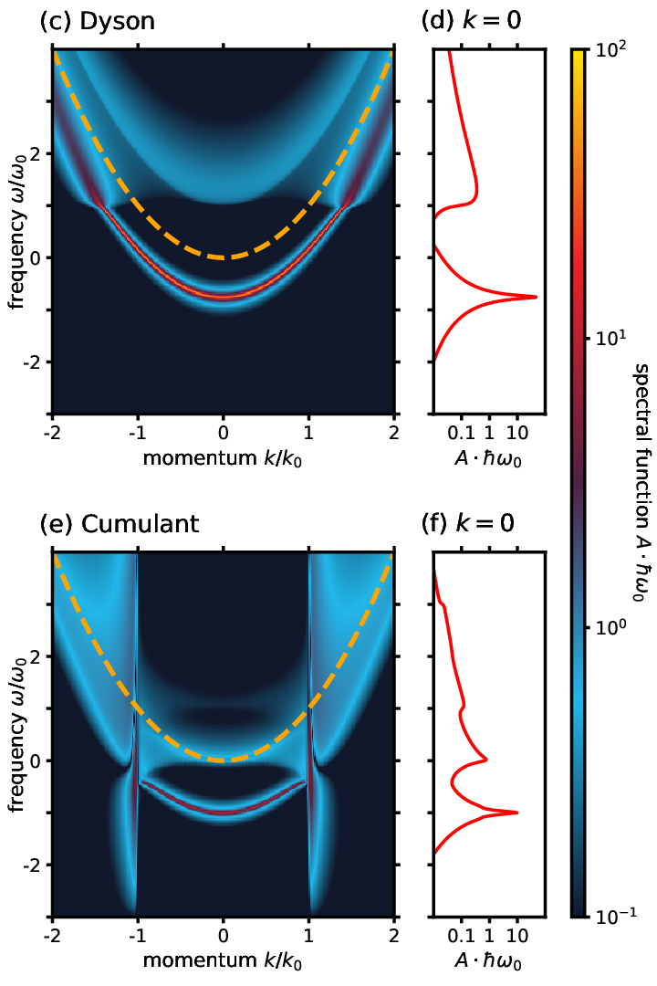
The real and imaginary parts of the self-energy are shown in Figs. 2(a) and (b), respectively. As the real part of the self-energy is negative everywhere [see Fig. 2(a)] the QP energy near the bottom of the conduction band lies below the non-interacting energy. The physical interpretation of this result is that the phonon cloud tends to stabilize the electron, precisely as it happens when a polaron is formed.Franchini et al. 2021 This qualitative trend holds for both the Dyson’s approach and the cumulant approach, as it can be seen in the spectral functions reported in Figs. 2(c), (d), and (e), (f), respectively.
The imaginary part of the self-energy vanishes identically for frequencies below the threshold , as it can be seen in Fig. 2(b). The interpretation of this behavior is that the electron does not have sufficient energy to emit a phonon, therefore its lifetime is infinite and . This effect is also seen in the spectral functions, Figs. 2(c) - (f), which exhibit sharp QP peaks for energies within from the band bottom.
Despite sharing the same self-energy, the Dyson and cumulant approaches differ considerably in the QP energies and effective masses. In the Dyson approach, the QP energy is defined by:
| (29) |
This expression does not lead to a general analytic expression for , but the QP energy and mass at the band bottom () have simple expressions, see e.g. Section 7.1.1 of Ref. 27:
| (30) |
and
| (31) |
The weak coupling () expansion of Eq. (30) can be obtained by writing the solution as a continued fraction and then taking the limit of small :
| (32) |
Similarly, the weak-coupling expansion of Eq. (31) is
| (33) |
The effective mass renormalization in the Dyson approach is the same as that obtained within Brillouin-Wigner perturbation theory applied to the Fröhlich polaron problem.Mahan 1993
In the case of the cumulant approach, the QP energy is given by:
| (34) |
By taking the limit of small , we obtain the standard result for the QP energy at the band bottom,
| (35) |
which is valid at all . The corresponding effective mass is:
| (36) |
These last two results coincide with what one obtains by performing Rayleigh-Schrödinger perturbation theory on the Fröhlich polaron problem.Schiff 1955
It is instructive to compare Eqs. (30), (33), (35), and (36) with calculations based on Feynman’s path integral approach to the Fröhlich polaron problem.Feynman 1955 Feynman’s approach is considered to be the most accurate in describing the undoped Fröhlich model, and agrees closely with advanced diagrammatic Monte Carlo calculations.Mishchenko et al. 2000 In this approach, the QP energy and mass at weak coupling are found to be:
| (37) |
| (38) |
These two results show that, at weak coupling (), both the Dyson approach and the cumulant approach yield QP energies and effective masses that agree with Feynman’s path integral calculation to first order in the coupling strength . A detailed comparison between these three approaches to the undoped Fröhlich model is shown in Fig. 3. This comparison shows that, while the three approaches agree at weak coupling, there exist significant differences for larger values of . In particular, the cumulant method yields a QP energy that remains closer to the Feynman result up to intermediate coupling strengths (), while the Dyson approach deviates from Feynman’s already at moderate coupling. On the other hand, the cumulant approach yields an unphysical divergence of the effective mass at intermediate coupling (singularity at and change of sign beyond this point), while the mass in Dyson’s method remains finite.
Based on the comparison between QP energies, recently it has been argued that the cumulant method provides a better description of polarons than Dyson’s approach.Nery et al. 2018 However, Fig. 3 clearly shows that the effective mass (and by extension the band structure) in the cumulant approach is not reliable at intermediate coupling. This point is further corroborated by a close inspection of the spectral functions in Fig. 2(e): As a result of a logarithmic singularity in the self-energy [Eq. (28)], the QP energy diverges when , and the spectral function exhibits unphysical vertical streaks.
Moving to the polaron satellites, we see from Figs. 2(c) and (e) that both the Dyson’s approach and the cumulant approach exhibit satellites states. As already discussed in numerous reports,Aryasetiawan et al. 1996; Lischner et al. 2013; Kas et al. 2014; Lischner et al. 2014; Story et al. 2014; Caruso and Giustino 2015; Caruso et al. 2015; Lischner et al. 2015; Zhou et al. 2015; Caruso and Giustino 2016b; Gumhalter et al. 2016; Vigil-Fowler et al. 2016; Verdi et al. 2017; Nery et al. 2018; Zhou et al. 2018; Zhou and Bernardi 2019; Antonius et al. 2020; Tzavala et al. 2020; Zhou et al. 2020; Chang et al.; Zhou et al. Dyson’s approach yields only one satellite, to leading order located at a binding energy of from the QP peak, see Fig. 2(c). On the other hand, the cumulant method correctly yields multiple satellites which are separated from the QP peak by integer multiples of the boson energy . Thus, the cumulant method is superior in the description of satellite features, as anticipated.
One last issue that deserves attention is the location of the satellites with respect to the QP band. Both Dyson’s method and the cumulant approach yield satellites located at higher energy than the QP band [see Figs. 2(c) and (e)] when applied to the empty-band system. However, in ARPES experiments satellites are observed below the QP band, as schematically illustrated in Fig. 1. This discrepancy has to do with the fact that ARPES probes occupied electronic states, while the empty-band Fröhlich model describes unoccupied states. It is clear that a correct description of polaron physics as probed in ARPES experiments necessitates the study of a doped Fröhlich solid. The following sections are devoted to the doped model.
III.2 Finite Fermi level in the conduction band
Now we consider the case of partially occupied conduction band with a Fermi energy . The self-energy for this case is obtained by setting in Eqs. (18) and (19). In this section, we ignore free-carrier screening, which will be included in Sec. III.3. This approximation is meaningful to describe the anti-adiabatic regime, where the Fermi level is much smaller than the characteristic phonon energy, .
After carrying out the integrals in Eqs. (18) and (19) explicitly, we obtain the following self-energies. For completeness, key steps of the derivation are provided in Appendix B. The lesser self-energy, which describes electron removal processes, is given by
with
| (40) | |||||
In these expressions, the auxiliary function is defined as:
| (41) | |||||
Li2 denotes the dilogarithm function, and are complex-valued parameters. The greater self-energy, which describes electron addition processes, is found to be:
| (42) | |||||
with
| (43) |
For metallic systems, Luttinger’s theorem states that the volume of the Fermi surface does not change when adiabatically turning on many-body interactions in a non-interacting system.Luttinger 1960 In the present model, the volume of the Fermi surface is determined by the Fermi wavevector , therefore Luttinger’s theorem implies that and hence the Fermi energy should not be affected by the self-energy . In order to enforce this condition, we subtracted the constants defined in Eqs. (40) and (III.2) from the lesser and greater self-energies in Eqs. (III.2) and (42), respectively, so that . One can verify that this choice leaves the QP energy at the Fermi level identical to the non-interacting energy, for both the Dyson’s and cumulant approaches.
Using Eqs. (III.2) and (42), the retarded self-energy is obtained as . We note that Eq. (42) correctly reduces to the corresponding equation for the undoped model, Eq. (28), upon taking the limit . The real and imaginary parts of the doped self-energy are shown in Figs. 4(a) and (b). The real self-energy is now positive in the range of occupied states, passes through zero at to ensure particle number conservation, and becomes negative for unoccupied states. The resulting QP peak shown in Figs. 4(c) and (e) thus exhibits a higher effective mass than the bare electron. In fact, we find that the mass renormalization in the presence of doping is even more pronounced than in the empty-band model, as we discuss below.
Turning to the imaginary self-energy shown in Fig. 4(b), we note that the main peak structure in for occupied states, , is now found at lower energies than the independent particle, causing the satellites in Figs. 4(c) and (d) to appear below the QP peak. For empty states, the situation is similar to the discussion of the empty-band model in Sec. (III.1), i.e. we find satellite features above the QP dispersions.
In both Dyson’s and cumulant approaches we find that QP energy and effective mass are strongly doping-dependent. Starting with the Dyson approach, the dressed electron energy is found to be:
| (44) | |||||
At the bottom of the conduction band , this result yields the following expressions for the QP energy and the effective mass:
| (45) | |||||
and
| (46) | |||
As in the undoped case, all quantities in the Dyson approach are defined self-consistently. In the cumulant approach, the QP energy and effective mass are again evaluated at the independent particle energy, and the self-energy is always linear in . The -dependent QP energy in the cumulant approach is given by:
| (47) | |||||
At the point, this becomes:
| (48) | |||
The cumulant effective mass is given by
| (49) | |||||
These expressions are illustrated in Fig. 6. The dependence of the QP renormalization on the coupling strength and doping level for the Dyson and cumulant approaches are shown in Figs. 6(a) and (c), respectively. Figures 6(b) and (d) show the corresponding effective masses.
The darker the shade of green in Figs. 6(a) and (c), the lower the QP energy lies below the Fermi level. This situation corresponds to a stable dressed electron, precisely as in the case of the undoped Fröhlich model. Conversely, the red areas in Figs. 6(a) and (c) indicate that the QP peak would lie above , causing a breakdown of the Fermi surface. This latter scenario is unphysical, and underscores the limitations of using a second-order electron-phonon self-energy.
Moreover, moving to the effective masses shown in Figs. 6(b) and (d), we find areas in the phase space where overshooting mass renormalization leads to an inversion of the curvature in the QP spectrum, and a negative effective mass (shown in red). We refer to this effect as ’anomalous mass enhancement’.
We emphasize that the data presented in Fig. 6 do not take into account free-carrier screening of the electron-phonon matrix elements. As we show in Sec. III.3 and Fig. 10, the inclusion of free-carrier screening extends the validity range of both the Dyson and cumulant approaches, but unphysical solutions still exist in the region , i.e. in the anti-adiabatic regime. The insets in Figs. 6(b) and (d) show an enlarged view of the low-doping limit for small . Note that the color bar has been extended with respect to the full image.
In fact, this situation is reminiscent of Fröhlich’s theory of superconductivity,Fröhlich 1950 which incorrectly predicts an inversion of the band curvature at strong coupling.Kohn and Vachaspati 1951 This artifact was later resolved within the Bardeen-Cooper-Schrieffer theory, where the self-energy is evaluated self-consistently as opposed to perturbatively,Bardeen et al. 1957 and the resulting band structure features an energy gap, instead of inverted bands.
The anomalous mass renormalization in the presence of doping, and the emergence of critical values for and is a consequence of an intricate dependence of on the Fermi energy: In appendix C, we show that the curvature of the (lesser) self-energy exhibits a singularity near . The effective mass is defined as:
| (50) |
and for . At large doping levels, the (negative) curvature of is small, and so is the mass enhancement due to Eq. (50). With decreasing , the curvature approaches from above, and the effective mass can reach arbitrarily large values. Beyond the critical value of , as the magnitude of keeps increasing, Eq. (50) becomes negative and the quasi-particle picture breaks down.
This behavior occurs in both the Dyson and cumulant aproaches, and is also independent of the specific implementation of the cumulant method: In appendix C, we show that the small- behavior of the retarded cumulantKas et al. 2014 is very similar.
It is instructive to consider the QP energy and mass renormalization near this singularity in . For small coupling strengths , we find the following expressions as we take the extreme anti-adiabatic limit in the Dyson approach:
| (51) |
| (52) |
while for the cumulant expansion we obtain:
| (53) |
| (54) |
Note that to obtain Eqs. (51)-(54), we have first taken the limit for small followed by the limit for small , i.e. we remain within the green area in Figs. 6(b) and (d).
Within the range of physical values for , we find that the Dyson approach tends to provide more stable solutions in the phase space, cf. Fig. 6. Nevertheless, given that for the doped Fröhlich solid there exists no solution equivalent to Feynman’s treatment of the Fröhlich polaron, it is difficult to judge whether the Dyson or cumulant approach yields the more accurate QP and mass renormalization.
For both approaches, we observe that combinations of intermediate-to-high coupling strengths and low doping levels quickly become problematic, while high doping levels and low coupling strengths lead to meaningful results. Probably, this was to be expected, since the Migdal theorem (which underpins the Fan-Migdal self-energy) is only valid within the adiabatic approximation, .Migdal 1958
This result is significant for the interpretation of experimental data. Commonly, the curvature of the QP band obtained from from ARPES measurements is used to determine the dressed mass and hence the coupling strength . In the literature, the coupling strength is often determined by using the formula for the undoped Fröhlich model, as given by Eqs. (31) and (36). However, the experimental setup for ARPES always requires a small but finite Fermi sea from which electrons can be excited. As discussed above, the physics of such a system are likely better captured by Eqs. (51)-(54).
Moving to the polaron satellites, we see from Figs. 4(c) and (d) that the Dyson approach again produces a single satellite starting with a broad area of low but non-zero spectral weight at one phonon energy below the Fermi edge. Note that this area extends beyond the Fermi momentum , suggesting that unoccupied electronic states could also emit a phonon upon excitation. This does not conform to experiment, and is an artefact of formulating the Fan-Migdal self-energy as a retarded quantity, i.e. treating occupied and unoccupied states within the same self-energy. At the lower end of the satellite structure, we recover a sharp peak whose intensity is almost of the order of the main QP peak.
On the other hand, the cumulant approach, shown in Figs. 4(e) and (f), produces several satellites at exactly integer multiples of the boson energy, with peak intensities following a Poisson distribution.
Moreover, our analytical approach indicates that the satellites consist of doublets: Consider Fig. 5, in which we juxtapose the imaginary self-energy at , also shown in Fig. 4(b), with the corresponding satellite function which yields the double-peaked satellite of Fig.4(e). At finite doping, phonon emission and absorption processes can occur at all energies between and , which causes the finite imaginary self-energy in the energy range . This is shown as the ’phonon’ line in blue in Fig. 5. Mathematically, this is due to the negative argument of the logarithm in Eq. (III.2) at the given values, which is independent of the electronic lifetime broadening . The energy of the lower edge of the satellite, , is equal to the singularity of the non-interacting electron Green’s function shifted by the phonon energy. This is indicated by the green line ’electron’ in Fig. 5. In numerical calculations, the peak height of this singularity is determined by the parameter , and it enters the self-energy through .
In some of the early work on the cumulant spectra of polarons, it was suspected that the satellite peak would simply follow the dispersion of the QP band.Caruso et al. 2018 By deriving all involved quantities analytically, we are able to uncover an even more nuanced picture of the cumulant satellites.
Conversely, our analytical solutions exhibit a secondary peak whose dispersion is inverted with respect to the main satellite peak, leading to a near-elliptical feature. The energy separation of the two structures that constitute the satellite peak equals the Fermi energy. This non-trivial satellite structure may be related to the finite spectral weight between satellites observed in experiment, and it could provide an explanation for some of the broadening of spectral features seen in ARPES but not yet reproduced in previous ab initio calculations; cf. e.g. Refs. 17; 19.
III.3 Finite Fermi level including free-carrier screening
In this last section we consider the most complex scenario: a Fröhlich model with doping as well as screening of the electron-phonon interaction by free carriers. Due to the intricate dependence of the screened matrix element on the wave vector , see Eq. (6), we express the screened self-energy in terms of a one-dimensional integral in . The screened lesser self-energy is given by:
| (55) |
with
| (56) |
The screened greater self-energy is found to be:
| (57) |
with
| (58) |
Expressions for the QP energy and effective mass for the screened case are provided in App. E.
The magnitude of electronic screening effects depends both on the given Fermi level , as well as material-specific parameters. In the Lindhard function in Eq. (4), system properties enter through the Wigner-Seitz radius , which depends on the bare mass of the conduction electrons and the dielectric constant of the undoped solid in the high-frequency limit.
In Fig. 7, we show the screening function as a function of doping level for two types of systems. This function quantifies the suppression of the electron-phonon matrix element by free-carrier screening, because the Fröhlich matrix elements appears to the second power in the self-energy, and the angular integration over the phonon wavevector introduces a phase-space factor . Therefore the impact of the screening is to modify a function that scales as to a function that scales as . If , there is no screening by free carriers; for , all electron-phonon coupling is completely suppressed. The dielectric function in Fig. 7(a) corresponds to a dilute electron gas with a high electron mass and intermediate dielectric constant, as realized e.g. in cubic SrTiO3. We observe that the ability of the free carriers to screen long-range (small-) electron-phonon coupling gradually increases over a typical doping range for conducting oxides (- cm-3). At the highest doping level shown, polar interactions are almost completely suppressed, indicating that we have reached the metallic limit.
By contrast, the screening function in Fig. 7(b) is that of a dense electron gas, as realized e.g. in GaAs. In the latter case, a very low electron mass means that the free carriers can screen long-range electron-phonon interactions very effectively already at relatively low doping levels. In these systems, Fröhlich coupling only plays a secondary role, therefore in the remainder of this manuscript we focus on dilute electron gases such as the one in Fig. 7(a).
Figure 8 illustrates the effect of this screening function on the real and imaginary parts of the self-energy at a doping level of . The corresponding unscreened and screened Dyson spectral functions are shown in Figs. 9(a)-(d), while the second-order cumulant spectral functions are shown in Figs. 9(e)-(h). In particular, note that the Fermi surface in the unscreened second-order cumulant spectrum in Fig. 9(e) is breaking down due to (unphysically) strong renormalization effects at the given values of and . We expect the effective electron-phonon interaction in a real system to be closer to the situation shown in Fig. 9(g), in which the polar coupling is partially suppressed.
Given the dependence of the dielectric function, the effect of electron screening is not uniform, but rather stronger up to a scattering wave vector , and then weaker for states and which are farther apart.
The significant effect of free-carrier screening on the total Fröhlich coupling strength in the system is also seen in Fig. 10, where we show the QP energy and effective mass renormalization in the doped Fröhlich solid using the screened matrix element. The comparison to the corresponding Fig. 6 is telling: We find that the region showing the effective mass anomaly is reduced, and in general we observe weaker renormalization for a wide range of coupling strengths and doping levels. For , the effective mass in the second-order cumulant expansion returns to values close to the non-interacting system.
Turning to the satellites in Figs. 9(a) and (c), we observe that the energy difference between QP and satellite in the screened system is reduced by approximately 50%. This result underscores the pathological dependence of the satellite energy on the coupling strength in Dyson’s approach. As the energy of the phonon is the same with or without screening (barring frequency renormalization effects that we did not consider in this work), there is no reason to expect the satellite energy to change as a result of free-carrier screening.
By contrast, the lower peak in the satellite structure in the screened cumulant spectrum [Fig. 9(g)] remains separated from the QP peak by one phonon energy. As discussed above, the energy span of the satellite in the cumulant approach matches the size of the Fermi energy in the system. At a Fermi level of =0.8, we find substantial spectral weight in the region in between the quasi-particle and the satellite. This finding is in remarkable agreement with the raw ARPES data reported in Refs. Wang et al. 2016; Riley et al. 2018 for -doped SrTiO3 and EuO, respectively.
IV Experimental QP weight
Wang et al.Wang et al. 2016 present a very careful analysis of polaron satellites in the two-dimensional electron gas in doped SrTiO3. The lowest doping level considered in this study is
cm-2. We can assume that the conduction band near is well described by three degenerate parabolic bands with an average band mass of .Devreese et al. 2010
The considered doping level then corresponds to a Fermi wavevector of =0.041 and a Fermi energy of meV. With a phonon energy of 100meV
and a reported Fröhlich coupling strength of , they observe intermediate quasi-particle renormalization with .
Equations (12) and (24) give the expressions for the Dyson and cumulant
quasi-particle weights, respectively. To be able to evaluate them analytically, we have derived expressions for the
frequency derivative of the self-energy for finite Fermi energy. For the Dyson equation approach, we need the
derivative of the full retarded self-energy:
| (59) | |||||
To obtain the Dyson quasi-particle weight at , we evaluate this expression at .
For the cumulant expansion, we find for the derivative:
| (60) |
We insert Eqs. (59) and (60) into Eqs. (12) and (24), and evaluate the quasi-particle weight using the parameters
The resulting quasi-particle weight is reported in table 2. We find that the calculated Dyson and cumulant QP weights over-estimate the measured weight by a factor of 2 and 1.5, respectively. For case of the cumulant expansion, this inconsistency between theoretical and experimental spectra has been studied in great detail in the literature, see e.g. Ref. 46. In this study, the authors are able to show how additional satellite intensity arises from inelastic scattering of the outgoing photoelectron in experiment.
V Conclusions
We have presented the doped Fröhlich solid as a generalization of the Fröhlich polaron problem to study the single-particle excitation spectra of doped polar oxides, as measured by ARPES experiments. To reach reliable conclusions that are not affected by numerical sampling of the electron-phonon scattering, we derived exact analytical expressions for the electron self-energy in the presence of free carriers. These expressions allow to analyze in detail the role of Pauli blocking and free carrier screening in the electron spectral functions.
Our analytical approach has provided new insight into the Fröhlich polaron problem, and allows us to draw the following conclusions: To capture the low-energy many-body physics of doped polar semiconductors, especially in the presence of doping (as needed in ARPES measurements), it is crucial to explicitly account for the small but non-zero electron occupations in the conduction band. We have demonstrated that neglecting finite occupations leads to incorrect satellite energetics and excessive electron-phonon renormalization. In the case of high doping levels, further many-body effects in the form of free-carrier screening of the electron-phonon matrix element must also be included to achieve a meaningful description of QP shifts and effective mass renormalization.
We have derived analytical expressions for the renormalized band energy and effective mass of the doped Fröhlich model, and investigated the dependence of these quantities on the coupling strength and the doping level. We have found that a significant portion of the coupling-doping phase diagram exhibits regions with anomalously strong mass enhancement, as well as regions where the band curvature is inverted, leading to a breakdown of the QP picture. These findings indicate that caution must be used when studying electron-phonon coupling in doped polar materials, as the standard second-order Fan-Migdal self-energy might not provide a physically accurate picture in the anomalous regions of the phase diagram identified in this work.
We also found that, in the presence of doping, the mass renormalization depends both on the electron-phonon coupling strength and the Fermi level. This finding implies that the use of the standard relation for extracting the Fröhlich coupling from experiments is not justified, and should be replaced by the generalized expression obtained in this work, Eq. (51).
In line with previous literature, we found that the second-order cumulant spectral function improves the description of polaron satellites compared to the conventional first-order Dyson approach. The intensity and binding energy of the sidebands provided by the cumulant method are in line with the equidistant satellites observed in experiments. On the other hand, the cumulant method appears to provide a worse description of the QP band, as compared to the Dyson approach. Indeed, we have shown that the cumulant approach leads to an inversion of the band curvature over a much wider region of the phase diagram as compared to the Dyson method, and that the cumulant spectral function exhibits unphysical vertical streaks that are intrinsic to the theoretical framework (rather than being numerical artifacts). Our comparative analysis of the cumulant and Dyson approaches leads to suggest that a complete description of the Fröhlich problem in the presence of doping might require the inclusion of self-energy diagrams beyond the second order. In the meantime, we recommend that both approaches be tested in future calculations, keeping in mind that the cumulant method appears more suited to describing satellites, and the Dyson method appears to describe QP bands better.
We hope that this work will stimulate further discussion on the role of doping in the electron-phonon interaction in polar insulators and semiconductors, and inspire additional investigations of the reliability and scope of the cumulant method and the Dyson approach in the study of electron-phonon effects in these materials.
Acknowledgements
This work was supported by the Computational Materials Sciences Program funded by the U.S. Department of Energy, Office of Science, Basic Energy Sciences, under Award DE-SC0020129. The authors acknowledge the Texas Advanced Computing Center (TACC) at The University of Texas at Austin for providing HPC resources via the Frontera LRAC project DMR21002, and the U.S. Department of Energy Office of Science User Facility at Lawrence Berkeley National Laboratory for providing resources via the National Energy Research Scientific Computing Center, NERSC award ERCAP0016747.
Appendix A Debye-Waller self-energy
In this appendix, we show that the QP shift arising from the Debye-Waller self-energyGiustino 2017 vanishes in the Fröhlich model. We start from the compact expression for the Debye-Waller matrix element in the rigid-ion approximation derived in Ref.77:
| (61) |
where , are Cartesian coordinates, is the atomic index, are the Bloch-periodic components of the electron wavefunctions, is the long-range part of the interaction potential, and
| (62) |
is the dipole moment in direction arising from the displacement of atom with Born effective charge along the direction . The potential derivative in Eq.(61) is defined asGiustino 2017
| (63) |
where is the lattice vector of the -th unit cell in the supercell, and is the coordinate of atom in cartesian direction .
In the doped Fröhlich solid, the electronic states are planewaves and the long-range part of the Fröhlich potential is Verdi and Giustino 2015
| (64) | |||||
Here, G is a reciprocal lattice vector, and is the static dielectric tensor of the crystal. Using the isotropy of our system to simplify the Born effective charge and dielectric tensors, and , we can calculate the derivative
| (65) |
After calculating the commutator of this function with the dipole , we obtain a lattice periodic expression, and as the eigenstates of our system are plane waves, we find
| (66) |
This result shows that the Debye-Waller correction vanishes for the Fröhlich model.
Appendix B Derivation of the Fan-Migdal self-energy
In this appendix, we outline the derivation of the various self-energy expressions used in this manuscript, starting from the definition of the Fan-Migdal self-energy given in Eqs. (18) and (19).
B.1 Single electron in the conduction band
In the case of a single electron added to the conduction band, the occupation factor vanishes everywhere, cancelling all contributions from the lesser self-energy.
At the point (), we integrate Eq. (19) by introducing spherical coordinates. We write:
| (67) |
and find:
| (68) |
where we used the definition of the Fröhlich matrix element, Eq. (2). Equation (67) leads directly to Eq. (30).
For general , we write Eq. (19) as
| (69) |
After transforming to spherical coordinates, we use the identity
| (70) |
and the definition of the Fröhlich matrix element, Eq. (2), to obtain:
The integrand in Eq. (B.1) has the primitive:
| (72) | |||||
We find ; in the limit , only the dilogarithms survive and converge to:
| (73) |
Inserting Eq. (73) into Eq. (B.1), we find Eq. (28) from the main text.
B.2 Finite Fermi level in the conduction band
We now consider the scenario where we have a finite electron density in the conduction band. At , the lesser self-energy is defined as
| (74) |
which can be integrated to give
| (75) |
For the greater self-energy, we have
| (76) |
and hence
For general , the lesser self-energy is obtained from an expression similar to that of Eq. (72), but with the sign of inverted, which then needs to be evaluated at and at , respectively, to give Eq. (III.2). The greater self-energy at is obtained from Eq. (72) evaluated at and , which leads to Eq. (42).
B.3 Finite Fermi level including free-carrier screening
In this section we provide details on the calculation of the self-energy in the presence of free-carrier screening. Inserting the screened coupling matrix element given in Eq. (19) into Eqs. (18) and (19), we obtain for the self-energy at :
| (78) |
| (79) |
Using the Fröhlich matrix element in Eq. (2), we recover Eqs. (III.3) and (III.3) from the main text.
For general , we write
| (80) | |||||
| (81) | |||||
where and are relative angles between vectors k and q. For the integration over angle , we use the substitution to obtain:
| (82) | |||||
| (83) | |||||
As we are using spherical coordinates, we have
, and , and hence
| (84) |
allowing us to identify three ranges for the integration over : For the lesser self-energy [Eq. (82)] we have: (i) If , then and
| (85) |
(ii) If , we have
| (86) |
(iii) For , the Heaviside function in (82) vanishes everywhere. In particular, there is no contribution for . Combining Eqs. (82), (85) and (86), we recover Eq. (III.3) from the main text.
Appendix C Derivation of the effective mass
C.1 Dyson effective mass
The effective mass corresponding to the QP energy in Dyson’s approach,
| (89) |
is given at by
| (90) |
We can express the momentum dependence of the self-energy in terms of the associated bare electron energy , and write:
| (91) |
and henceSchlipf et al. 2018
| (92) |
C.2 Cumulant effective mass
As the QP energy in the cumulant expansion is simply given by
| (93) |
the corresponding effective mass is equal to
| (94) |
As the cumulant self-energy is linear in , the small- expansion of the effective mass becomes
| (95) |
C.3 Singularity in
C.4 Effective mass of the retarded cumulant
In the framework of the retarded cumulant, the effective mass at is defined as:
| (98) |
where is now the full retarded self-energy introduced in Eq. (13). Following the same steps as before, one finds for the expansion to first order in :
| (99) | |||||
Taking the limit , we reach
| (100) |
which has the same behavior for small as Eq. (54) in the main text.
Appendix D Small-coupling limits, Dyson approach
Appendix E Renormalized quantities including free-carrier screening
Upon including free-carrier screening, the Dyson QP energy can be expressed in terms of the one-dimensional integral
| (103) | |||||
In particular, the occupied state at the band bottom becomes
| (104) | |||
The effective mass at the zone center is given by:
To linear order in , the weak-coupling limit of Eq. (104) is simply given by:
| (106) |
For Eq. (E), we find at small :
| (107) | |||||
In the case of the cumulant approach, the QP energy for is given by
| (108) | |||||
In the limit , we recover
| (109) | |||
which is already linear in . Lastly, the cumulant effective mass at is given by:
| (110) |
and its small- expansion is equal to
| (111) | |||
References
- Fröhlich et al. (1950) H. Fröhlich, H. Pelzer, and S. Zienau, The London, Edinburgh, and Dublin Philosophical Magazine and Journal of Science 41, 221 (1950).
- (2) J. T. Devreese, arXiv:cond-mat/0004497 .
- Devreese and Alexandrov (2009) J. T. Devreese and A. S. Alexandrov, Rep. Prog. Phys. 72, 066501 (2009).
- Verdi and Giustino (2015) C. Verdi and F. Giustino, Phys. Rev. Lett. 115, 176401 (2015).
- Sjakste et al. (2015) J. Sjakste, N. Vast, M. Calandra, and F. Mauri, Phys. Rev. B 92, 054307 (2015).
- Park et al. (2020) J. Park, J.-J. Zhou, V. A. Jhalani, C. E. Dreyer, and M. Bernardi, Phys. Rev. B 102, 125203 (2020).
- Brunin et al. (2020) G. Brunin, H. P. C. Miranda, M. Giantomassi, M. Royo, M. Stengel, M. J. Verstraete, X. Gonze, G.-M. Rignanese, and G. Hautier, Phys. Rev. Lett. 125, 136601 (2020).
- Miglio et al. (2020) A. Miglio, V. Brousseau-Couture, E. Godbout, G. Antonius, Y.-H. Chan, S. G. Louie, M. Côté, M. Giantomassi, and X. Gonze, Npj Comput. Mater. 6, 167 (2020).
- Ohtomo and Hwang (2004) A. Ohtomo and H. Y. Hwang, Nature 427, 423 (2004).
- Herranz et al. (2007) G. Herranz, M. Basletić, M. Bibes, C. Carrétéro, E. Tafra, E. Jacquet, K. Bouzehouane, C. Deranlot, A. Hamzić, J.-M. Broto, A. Barthélémy, and A. Fert, Phys. Rev. Lett. 98, 216803 (2007).
- Schooley et al. (1964) J. F. Schooley, W. R. Hosler, and M. L. Cohen, Phys. Rev. Lett. 12, 474 (1964).
- Schooley et al. (1965) J. F. Schooley, W. R. Hosler, E. Ambler, J. H. Becker, M. L. Cohen, and C. S. Koonce, Phys. Rev. Lett. 14, 305 (1965).
- Lin et al. (2014) X. Lin, G. Bridoux, A. Gourgout, G. Seyfarth, S. Krämer, M. Nardone, B. Fauqué, and K. Behnia, Phys. Rev. Lett. 112, 207002 (2014).
- Meevasana et al. (2011) W. Meevasana, P. D. C. King, R. H. He, S.-K. Mo, M. Hashimoto, A. Tamai, P. Songsiriritthigul, F. Baumberger, and Z.-X. Shen, Nat. Mater. 10, 114 (2011).
- Santander-Syro et al. (2011) A. F. Santander-Syro, O. Copie, T. Kondo, F. Fortuna, S. Pailhès, R. Weht, X. G. Qiu, F. Bertran, A. Nicolaou, A. Taleb-Ibrahimi, P. Le Fèvre, G. Herranz, M. Bibes, N. Reyren, Y. Apertet, P. Lecoeur, A. Barthélémy, and M. J. Rozenberg, Nature 469 (2011).
- Chen et al. (2015) C. Chen, J. Avila, E. Frantzeskakis, A. Levy, and M. C. Asensio, Nat. Commun. 6, 8585 (2015).
- Wang et al. (2016) Z. Wang, S. McKeown Walker, A. Tamai, Y. Wang, Z. Ristic, F. Y. Bruno, A. de la Torre, S. Riccò, N. C. Plumb, M. Shi, P. Hlawenka, J. Sánchez-Barriga, A. Varykhalov, T. K. Kim, M. Hoesch, P. D. C. King, W. Meevasana, U. Diebold, J. Mesot, B. Moritz, T. P. Devereaux, M. Radovic, and F. Baumberger, Nat. Mater. 15 (2016).
- Moser et al. (2013) S. Moser, L. Moreschini, J. Jaćimović, O. S. Barišić, H. Berger, A. Magrez, Y. J. Chang, K. S. Kim, A. Bostwick, E. Rotenberg, L. Forró, and M. Grioni, Phys. Rev. Lett. 110, 196403 (2013).
- Riley et al. (2018) J. M. Riley, F. Caruso, C. Verdi, L. B. Duffy, M. D. Watson, L. Bawden, K. Volckaert, G. van der Laan, T. Hesjedal, M. Hoesch, F. Giustino, and P. D. C. King, Nat. Comm. 9 (2018).
- Husanu et al. (2020) M.-A. Husanu, L. Vistoli, C. Verdi, A. Sander, V. Garcia, J. Rault, F. Bisti, L. L. Lev, T. Schmitt, F. Giustino, A. S. Mishchenko, M. Bibes, and V. N. Strocov, Commun. Phys 3, 62 (2020).
- Yukawa et al. (2016) R. Yukawa, K. Ozawa, S. Yamamoto, H. Iwasawa, K. Shimada, E. F. Schwier, K. Yoshimatsu, H. Kumigashira, H. Namatame, M. Taniguchi, and I. Matsuda, Phys. Rev. B 94, 165313 (2016).
- Lee et al. (2014) J. J. Lee, F. T. Schmitt, R. G. Moore, S. Johnston, Y.-T. Cui, W. Li, M. Yi, Z. K. Liu, M. Hashimoto, Y. Zhang, D. H. Lu, T. P. Devereaux, D.-H. Lee, and Z.-X. Shen, Nature 515, 245 (2014).
- Cancellieri et al. (2016) C. Cancellieri, A. S. Mishchenko, U. Aschauer, A. Filippetti, C. Faber, O. S. Barisic, V. A. Rogalev, T. Schmitt, N. Nagaosa, and V. N. Strocov, Nat. Commun. 7, 10386 (2016).
- Giustino (2017) F. Giustino, Rev. Mod. Phys. 89, 015003 (2017).
- Story et al. (2014) S. M. Story, J. J. Kas, F. D. Vila, M. J. Verstraete, and J. J. Rehr, Phys. Rev. B 90, 195135 (2014).
- Migdal (1958) A. B. Migdal, Sov. Phys. JETP 7, 996 (1958).
- Mahan (1993) G. D. Mahan, Many-Particle Physics, 2nd ed. (Plenum Publishers, New York, 1993).
- (28) T. M. Bretz-Sullivan, A. Edelman, J. S. Jiang, A. Suslov, D. Graf, J. Zhang, G. Wang, C. Chang, J. E. Pearson, A. B. Martinson, P. B. Littlewood, and A. Bhattacharya, arXiv:1904.03121 .
- Verdi et al. (2017) C. Verdi, F. Caruso, and F. Giustino, Nat. Commun. 8, 15769 (2017).
- Nery et al. (2018) J. P. Nery, P. B. Allen, G. Antonius, L. Reining, A. Miglio, and X. Gonze, Phys. Rev. B 97, 115145 (2018).
- Zhou and Bernardi (2019) J.-J. Zhou and M. Bernardi, Phys. Rev. Res. 1, 033138 (2019).
- Langreth (1970) D. C. Langreth, Phys. Rev. B 1, 471 (1970).
- Hedin (1980) L. Hedin, Physica Scripta 21, 477 (1980).
- Aryasetiawan et al. (1996) F. Aryasetiawan, L. Hedin, and K. Karlsson, Phys. Rev. Lett. 77, 2268 (1996).
- Lischner et al. (2013) J. Lischner, D. Vigil-Fowler, and S. G. Louie, Phys. Rev. Lett. 110, 146801 (2013).
- Kas et al. (2014) J. J. Kas, J. J. Rehr, and L. Reining, Phys. Rev. B 90, 085112 (2014).
- Caruso and Giustino (2015) F. Caruso and F. Giustino, Phys. Rev. B 92, 045123 (2015).
- Caruso et al. (2015) F. Caruso, H. Lambert, and F. Giustino, Phys. Rev. Lett. 114, 146404 (2015).
- Caruso and Giustino (2016a) F. Caruso and F. Giustino, Phys. Rev. B 94, 115208 (2016a).
- Caruso and Giustino (2016b) F. Caruso and F. Giustino, Eur. Phys. J B 89, 238 (2016b).
- Gumhalter et al. (2016) B. Gumhalter, V. Kovač, F. Caruso, H. Lambert, and F. Giustino, Phys. Rev. B 94, 035103 (2016).
- Zhou et al. (2018) J. S. Zhou, M. Gatti, J. J. Kas, J. J. Rehr, and L. Reining, Phys. Rev. B 97, 035137 (2018).
- Tzavala et al. (2020) M. Tzavala, J. J. Kas, L. Reining, and J. J. Rehr, Phys. Rev. Research 2, 033147 (2020).
- Caruso et al. (2018) F. Caruso, C. Verdi, S. Poncé, and F. Giustino, Phys. Rev. B 97, 165113 (2018).
- Antonius et al. (2020) G. Antonius, Y.-H. Chan, and S. G. Louie, Phys. Rev. Res. 2, 043296 (2020).
- Zhou et al. (2020) J. S. Zhou, L. Reining, A. Nicolaou, A. Bendounan, K. Ruotsalainen, M. Vanzini, J. J. Kas, J. J. Rehr, M. Muntwiler, V. N. Strocov, F. Sirotti, and M. Gatti, Proc. Nat. Acad. Sci. USA 117, 28596 (2020).
- Lee and Pines (1952) T.-D. Lee and D. Pines, Phys. Rev. 88, 960 (1952).
- Röseler (1968) J. Röseler, Phys. Status Solidi B 25, 311 (1968).
- Smondyrev (1986) M. Smondyrev, Theor. Math. Phys. 68 (1986).
- Selyugin and Smondyrev (1989) O. V. Selyugin and M. A. Smondyrev, Phys. Status Solidi B 155, 155 (1989).
- Feynman (1955) R. P. Feynman, Phys. Rev. 97, 660 (1955).
- Prokof’ev and Svistunov (1998) N. V. Prokof’ev and B. V. Svistunov, Phys. Rev. Lett. 81, 2514 (1998).
- Mishchenko et al. (2000) A. S. Mishchenko, N. V. Prokof’ev, A. Sakamoto, and B. V. Svistunov, Phys. Rev. B 62, 6317 (2000).
- Hedin and Lundqvist (1969) L. Hedin and S. Lundqvist, Solid State Phys. 23, 1 (1969).
- Damascelli et al. (2003) A. Damascelli, Z. Hussain, and Z.-X. Shen, Rev. Mod. Phys. 75, 473 (2003).
- Abrikosov et al. (1975) A. Abrikosov, L. P. Gor’kov, and I. Dzyaloshinski, Methods of Quantum Field Theory in Statistical Physics (Dover, New York, 1975).
- Allen and Heine (1976) P. B. Allen and V. Heine, J. Phy. C 9, 2305 (1976).
- Allen (1978) P. B. Allen, Phys. Rev. B 18, 5217 (1978).
- Marini (2008) A. Marini, Phys. Rev. Lett. 101, 106405 (2008).
- Giustino et al. (2010) F. Giustino, S. G. Louie, and M. L. Cohen, Phys. Rev. Lett. 105, 265501 (2010).
- Antonius et al. (2014) G. Antonius, S. Poncé, P. Boulanger, M. Côté, and X. Gonze, Phys. Rev. Lett. 112, 215501 (2014).
- Aryasetiawan (2000) F. Aryasetiawan, in Strong Coulomb Correlations in Electronic Structure Calculations, Vol. 1, edited by V. Anisimov (CRC Press, Boca Raton, 2000).
- Schlipf et al. (2018) M. Schlipf, S. Poncé, and F. Giustino, Phys. Rev. Lett. 121, 086402 (2018).
- Franchini et al. (2021) C. Franchini, M. Reticcioli, M. Setvin, and U. Diebold, Nat. Rev. Mater. 6, 560 (2021).
- Schiff (1955) L. I. Schiff, Quantum Mechanics, 2nd ed. (McGraw-Hill, New York, 1955).
- Lischner et al. (2014) J. Lischner, D. Vigil-Fowler, and S. G. Louie, Phys. Rev. B 89, 125430 (2014).
- Lischner et al. (2015) J. Lischner, G. K. Pálsson, D. Vigil-Fowler, S. Nemsak, J. Avila, M. C. Asensio, C. S. Fadley, and S. G. Louie, Phys. Rev. B 91, 205113 (2015).
- Zhou et al. (2015) J. S. Zhou, J. J. Kas, L. Sponza, I. Reshetnyak, M. Guzzo, C. Giorgetti, M. Gatti, F. Sottile, J. J. Rehr, and L. Reining, J. Chem. Phys. 143, 184109 (2015).
- Vigil-Fowler et al. (2016) D. Vigil-Fowler, S. G. Louie, and J. Lischner, Phys. Rev. B 93, 235446 (2016).
- (70) J.-J. Chang, Benjamin K.and Zhou, N.-E. L. Lee, and M. Bernardi, arXiv:2106.09810 .
- (71) J.-J. Zhou, J. Park, I. Timrov, A. Floris, M. Cococcioni, N. Marzari, and M. Bernardi, arXiv:2102.06840 .
- Luttinger (1960) J. M. Luttinger, Phys. Rev. 119, 1153 (1960).
- Fröhlich (1950) H. Fröhlich, Phys. Rev. 79, 845 (1950).
- Kohn and Vachaspati (1951) W. Kohn and Vachaspati, Phys. Rev. 83, 462 (1951).
- Bardeen et al. (1957) J. Bardeen, L. N. Cooper, and J. R. Schrieffer, Phys. Rev. 108, 1175 (1957).
- Devreese et al. (2010) J. T. Devreese, S. N. Klimin, J. L. M. van Mechelen, and D. van der Marel, Phys. Rev. B 81, 125119 (2010).
- Lihm and Park (2020) J.-M. Lihm and C.-H. Park, Phys. Rev. B 101, 121102 (2020).
| Dyson | Dyson | Cumulant | ||||||
|---|---|---|---|---|---|---|---|---|
| Single electron | (29) | (30) | (31) | (32) | (33) | (34) | (35) | (36) |
| Finite doping | (44) | (45) | (46) | (101) | (102) | (47) | (48) | (49) |
| Doping and screening | (103) | (104) | (E) | (E) | (107) | (108) | (109) | (E) |
| Experiment Wang et al. 2016 | Dyson | Cumulant | |
| QP weight | 0.2 | 0.38 | 0.31 |