Inferring the neutron star maximum mass and lower mass gap in neutron star–black hole systems with spin

It remains unclear whether NSs, specifically those in merging BNS and NSBH systems, can have significant spins. The most rapidly spinning NS in a (nonmerging) double NS system is the Pulsar J1807-2500B with a period of 4.2 ms or dimensionless spin magnitude $a=0.12$ (Lynch et al. 2012). Among recycled pulsars, the fastest spinning is Pulsar J1748-2446ad with a period of $\sim 1.4$ ms (Hessels et al. 2006). However, rapidly spinning NSs in which spin down is inefficient (due to e.g. weak magnetic fields) may have avoided electromagnetic discovery for the same reasons. In NSBH systems, it may also be possible for the NS spin to grow through accretion if the NS is born before the BH (Chattopadhyay et al. 2021), or through tidal synchronization as has been studied in BBH systems  (Qin et al. 2018).

We remain agnostic about NS spin magnitudes, modeling their distribution as a power law,

where $a_{\mathrm{max}}$ sets an upper limit on possible values of $a_{2}$ and $\beta_{s}$ controls the slope. For $\beta_{s}=0$, the secondary spin magnitude follows a uniform distribution; for $\beta_{s}>0$, the secondary spin distribution prefers low spin. The maximum value of $a_{\mathrm{max}}$ is the breakup spin $a_{\text{Kep}}$, which is around $a_{\text{Kep}}\approx 0.7$ for most EOSs.

We do not explicitly model NS spin tilts (the angle between the spin vector and the orbital angular momentum axis), but consider a few different assumptions and explore how they affect our inference. By default, we consider a NS spin tilt distribution that is isotropic, or flat in $-1<\cos(\mathrm{tilt}_{2})<1$. We also explore a restricted model in which NS spins are perfectly aligned with the orbit, $\cos(\mathrm{tilt}_{2})=1$. For the distribution of BH spins, by default we assume that BHs are nonspinning (Fuller and Ma 2019; Mandel and Smith 2021, $a_{1}=0$;). We alternatively assume that the BH spin distribution is uniform in spin magnitude with isotropic spin tilts.

In summary, we consider the following spin models:

1. 1.

   Zero spin BH (“ZS”, default spin model): Primary BH is nonspinning ($a_{1}=0$). Secondary NS spin is isotropic in spin tilt (flat in $-1<\cos(\mathrm{tilt}_{2})<1$) and follows a power law in the spin magnitude $a_{2}$ (Eq. 1).

2. 2.

   Zero spin BH + aligned spin NS (“ZS + AS”): Same as Default, but with $\cos(\mathrm{tilt}_{2})=1$.

3. 3.

   Uniform and isotropic (“U+I”): Same as Default, but primary BH spin is flat in magnitude $a_{1}$ and $\cos(\mathrm{tilt}_{1})$ rather than nonspinning.

Like the case with spins, we consider a few different mass models to check the robustness of our conclusions. We consider three models for NS masses, which describe the distribution of NSBH secondary masses $m_{2}$ (see Fig. 1):

1. 1.

   Default: Single Gaussian distribution (panels a, d–f of Figure 1)

   $$p(m_{2}|\mu,\sigma,M_{min},M_{max})=\\ \begin{cases}\mathcal{N}_{T}(m_{2}|\mu,\sigma)&M_{min}\leq m_{2}\leq M_{max}\\ 0&\mathrm{otherwise},\end{cases}$$

   where $\mathcal{N}_{T}(x\mid\mu,\sigma)$ denotes a truncated Gaussian distribution with mean $\mu$ and standard deviation $\sigma$.

2. 2.

   Two-component (bimodal) Gaussian distribution (“2C”), as in the Galactic NS distribution (Alsing et al. 2018, panel b of Figure1)

   $$p(m_{2}|\mathcal{A},\mu_{1},\sigma_{1},\mu_{2},\sigma_{2},M_{\mathrm{min}},M_{\mathrm{max}})=\\ \begin{cases}\mathcal{A}\mathcal{N}_{T}(m_{2}|\mu_{1},\sigma_{1})+\\ (1-\mathcal{A})\mathcal{N}_{T}(m_{2}|\mu_{2},\sigma_{2})&M_{\mathrm{min}}\leq m_{2}\leq M_{\mathrm{max}}\\ 0&\mathrm{otherwise}.\end{cases}$$

   (2)

3. 3.

   Uniform distribution (“U”) with sharp cutoffs at the minimum and maximum NS mass [$M_{\rm min},M_{\rm max}$] (panel c of Figure 1)

   $$p(m_{2}|M_{\mathrm{min}},M_{\mathrm{max}})=\\ \begin{cases}\frac{1}{M_{\mathrm{max}}-M_{\mathrm{min}}}&M_{\mathrm{min}}\leq m_{2}\leq M_{\rm max}\\ 0&\mathrm{otherwise}.\end{cases}$$

All normal distributions ($\mathcal{N}_{T}$) are truncated sharply and normalized to integrate to 1 between $M_{\text{min}}=1M_{\odot}$ and $M_{\text{max}}$. In this work, we focus on inferring the maximum NS mass. While the minimum NS mass can also be inferred with GWs (Chatziioannou and Farr 2020), we fix the minimum NS mass to $1\,M_{\odot}$ in our models. If binary stellar evolution can produce NSs with extreme masses, then $M_{\mathrm{min}}$ and $M_{\mathrm{max}}$ correspond to the minimum and maximum allowable masses set by nuclear physics.

Crucially, we allow NSs to have significant spin. Rapid uniform rotation may provide additional support to the NS, allowing it to reach masses greater than the non-spinning maximum mass $M_{TOV}$. We model the dependence of $M_{\mathrm{max}}$ on NS spin $a_{2}$ using the universal relationship from Most et al. 2020:

with $A_{2}=0.132$, $A_{4}=0.0071$, where $a_{\text{Kep}}$ corresponds to the dimensionless spin at the mass-shedding limit. For concreteness, we assume $a_{\mathrm{Kep}}=0.7$, which is true for most EOS. For a neutron star with spin $a_{\text{Kep}}$, the maximum possible mass is around $1.2\times$ the (non-spinning) TOV limit. To measure this relation directly from gravitational-wave data, we also optionally measure a free, linear dependence between maximum spin and critical mass (see Section IV.5):

The extent to which the NS mass distribution can extend above $M_{\text{TOV}}$ depends on the spin distribution. The NS mass distributions $p(m_{2})$ above include a dependence on spin, and can be written as $p(m_{2}|M_{\rm max}(a_{2}),\theta)$ where $\theta$ includes all other parameters. Figure 1d–f shows the NS mass distribution under three variations of the spin distributions outlined in II.1.1.

We model the primary (BH) mass distribution $p(m_{1})$ as a power law with slope $-\alpha$, and a minimum mass cutoff at $M_{\rm BH}$:

We fix $\alpha>0$ such that the probability density decreases for increasing BH mass. The minimum BH mass represents the upper boundary of the mass gap. In order to restrict the range of $m_{1}$ to reasonable values, we optionally include a maximum BH mass of $30\,M_{\odot}$ in Eq. 4. However, for most of our NSBH models, high-mass BHs are rare due to a relatively steep slope $\alpha$ and/or a pairing function that disfavors extreme mass ratio pairings, and we do not explicitly model the BH maximum mass.

We assume that the pairing function between $m_{1}$ and $m_{2}$ NSBH systems follows a power law in the mass ratio $m_{2}/m_{1}=q<1$ (Fishbach and Holz 2020):

where by default we assume $\beta=0$ (Farah et al. 2021). We alternatively consider the case $\beta=3$, which favors equal-mass pairings. Depending on the width of the mass gap, NSBHs may necessarily have unequal masses, but on a population level, higher $q$ may still be relatively preferred.

Putting the mass and spin distributions together, we model the distribution of NSBH masses and spins $\theta\equiv(m_{1},m_{2},a_{1},a_{2})$ given population hyperparameters $\Lambda$ and model $H$ as:

where $H$ refers to the choice of model as described in the earlier subsections. For the extrinsic source parameters not in $\theta$, we assume isotropic distributions in sky position, inclination and orientation, and the local-Universe approximation to a uniform-in-volume distribution $p(d_{L})\propto d_{L}^{2}$, where $d_{L}$ is the luminosity distance.

We infer properties of the overall NSBH population with a hierarchical Bayesian approach (Loredo 2004; Mandel et al. 2019). This allows us to marginalize over the uncertainties in individual events’ masses and spins (grouped together in the set $\theta_{i}$ for event $i$) in order to estimate the hyperparameters $\Lambda$ describing the NS and BH mass and spin distributions. For $N_{det}$ GW detections producing data $d$, the likelihood of the data is described by an inhomogeneous Poisson process:

where $N$ is the total number of NSBH mergers in the Universe within some observing time, $\xi(\Lambda)$ is the fraction of detectable events in the population described by hyperparameters $\Lambda$ (see Section II.2.2), $\mathcal{L}({d_{i}|\theta_{i}})$ is the likelihood for event $i$ given its masses and spins $\theta_{i}$, and $\pi(\theta|\Lambda)$ describes the NSBH mass and spin distribution given population hyperparameters $\Lambda$ (Eq. 6. As we do not attempt to calculate event rates, we marginalize over $N$ with a log-uniform prior and calculate the population likelihood as (Mandel et al. 2019; Fishbach et al. 2018):

We evaluate the single-event likelihood $\mathcal{L}(d\mid\theta)$ via importance sampling over $N_{\text{samp}}$ parameter estimation samples $\theta_{\mathrm{PE}}$ for each event:

where $\pi_{\mathrm{PE}}(\theta)$ is the original prior that was used in LIGO parameter estimation. We calculate the posterior on the population parameters, $p(\Lambda\mid d)$, from the likelihood $\mathcal{L}(d\mid\Lambda)$, under Bayes theorem, using broad, flat priors on the parameters $\Lambda$. For prior ranges, see Table 1.

While we model and measure the astrophysical source distributions, GW detectors observe only sources loud enough to be detected, i.e. sources that produce data above some threshold $d>\mathrm{thresh}$. We account for this selection effect by including the term $\xi(\Lambda)$, the fraction of detectable binaries from a population described by parameters $\Lambda$.

To evaluate $\xi(\Lambda)$, we calculate the detection probability $P_{\mathrm{det}}(\theta)$ as a function of masses and cosmological redshift following the semi-analytic approach outlined in Fishbach and Holz 2017. We assume the detection threshold is a simple single-detector signal-to-noise ratio (SNR) threshold $\rho_{\mathrm{thresh}}=8$. We neglect the effect of spin on detectability; although systems with large aligned spins experience orbital hang-up that increases their SNR compared to small or anti-aligned spins, the effect is small compared to current statistical uncertainties (Ng et al. 2018).

Given masses and redshift of a potential source, we calculate its detectability as follow. We first calculate the optimal matched-filter SNR $\rho_{\text{opt}}$ using noise power spectral density (PSD) curves corresponding to aLIGO at O3 sensitivity, Design sensitivity, or A+ sensitivity (Abbott et al. 2020c); the optimal SNR corresponds to a face-on, directly-overhead source. We then calculate the SNR $\rho$ for a random sky position and orientation by generating angular factors $0<w<1$ from a single-detector antenna pattern (Finn and Chernoff 1993) and set $\rho=w\rho_{\text{opt}}$. If $\rho>\rho_{\mathrm{thresh}}$ for a given detector noise curve, we consider the simulated source to be detected.

Finally, we estimate $\xi(\Lambda)$ with a Monte Carlo integral over simulated sources. We draw simulated sources with $m_{1},m_{2},z$ according to $p_{\mathrm{draw}}(\theta)$ until injection sets of  10,000 events are created. BH ($m_{1}$) are drawn from a power law with $M_{\text{BH}}=1.5M_{\odot}$. NS ($m_{2}$) are drawn from a uniform distribution between $1$ and $3.5M_{\odot}$. Redshifts $z$ are drawn uniform in comoving volume and source-frame time. Each simulated system is labeled as detected or not based on its SNR, described above. We then approximate the integral $\xi(\Lambda)$ as a sum over $M_{\mathrm{det}}$ detected simulated systems:

While the population distributions in II.1 are defined in terms of $m_{1}$, $m_{2}$, $a_{1}$, and $a_{2}$, gravitational-wave detectors are most sensitive to degenerate combinations of these parameters. These include the gravitational chirp mass

the symmetric mass ratio

and $\chi_{\text{eff}}$, a mass-weighted sum of the component spins that is approximately conserved during the inspiral

where $a_{1,z}$ and $a_{2,z}$ are the components of the primary and secondary spin that are aligned with the orbital angular momentum axis. If the primary is nonspinning, $\chi_{\text{eff}}$ reduces to $\frac{m_{2}a_{2,z}}{m_{1}+m_{2}}=a_{2,z}\frac{q}{1+q}$.

We follow the method outlined in Chatziioannou and Farr 2020 to simulate realistic parameter estimation samples from mock GW NSBH detections. Chatziioannou and Farr 2020 use the post-Newtonian (PN) description of the GW inspiral, with PN coefficients $\psi_{0},\psi_{2}$, and $\psi_{3}$ that depend on the masses and spins.

where the mass difference $\delta m=(m_{1}-m_{2})/(m_{1}+m_{2})$ and the spin difference $\chi_{a}=(a_{1,z}-a_{2,z})/2$. The third coefficient $\psi_{3}$ encodes the spin-orbit degeneracy as $\beta$ includes the spins and $\nu$ is the mass ratio. In our case, unlike in Chatziioannou and Farr 2020, the $\chi_{a}$ term is not negligible. For NSBH systems, especially under the assumption of a spinning secondary and nonspinning primary, both the mass difference $\delta m$ and spin difference $\chi_{a}$ are significant. For our mock events, we approximate the measured PN coefficients $\psi_{i}$ as independent Gaussian distributions with standard deviations $\sigma_{i}$. As in Chatziioannou and Farr 2020, we adopt $\sigma_{0}=0.0046\psi_{0}/\rho$, $\sigma_{2}=0.2341\psi_{2}/\rho$, and $\sigma_{3}=-0.1293\psi_{3}/\rho$, where we draw the SNR $\rho$ according to $p(\rho)\propto\rho^{-4}$, an approximation to the SNR distribution of a uniform-in-comoving-volume distribution of sources (Chen and Holz 2014). We then sample $m_{1}$, $m_{2}$, $a_{1,z}$, and $a_{2,z}$ from the $\psi_{0}$, $\psi_{2}$, $\psi_{3}$ likelihoods, accounting for the priors induced by the change of variables by calculating the appropriate Jacobian transformations.

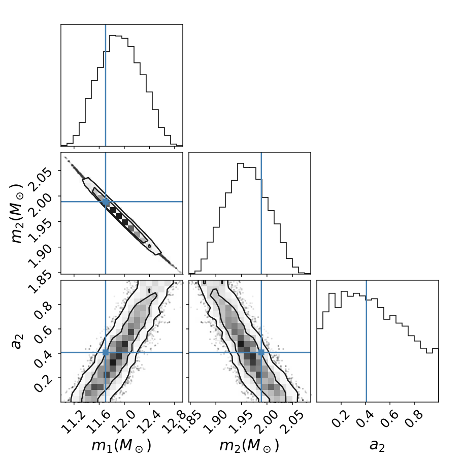
An example NSBH parameter estimation posterior generated according to this procedure is shown in Fig. 2. We see that the masses and spins are highly correlated. In particular, the anti-correlation between the secondary mass and spin increases the uncertainty on $M_{\mathrm{TOV}}$ and the spin–maximum mass relationship.

For each model and dataset variation, we infer the minimum BH mass $M_{\text{BH}}$, the NS $M_{\text{TOV}}$, and their difference (representing the width of the mass gap), marginalizing over all other parameters of the mass and spin distribution. Results for our Default model are shown in Figs. 5-10, with Fig.-10 showing a corner plot over all model parameters.

Maximum (spin-dependent) NS mass: As discussed in II.1.2, at a given secondary spin, we model a hard cut-off in the NS mass distribution $p(m_{2})$. However, in the 1-component and 2-component models, some values of $\mu$ and $\sigma$ taper off the mass distribution between 2–3 $M_{\odot}$, making it difficult to discern a sharp truncation mass $M_{\text{TOV}}$ from the function’s normal behavior. This results in long, flat tails to large posterior values of $M_{\text{TOV}}$ (see panel (a) of Fig. 5), reaching the prior bounds even if priors on $M_{\text{TOV}}$ are widened. A better measured parameter is the 99th percentile of the nonspinning NS mass distribution, $M_{99}$ (panel b of Fig. 5). For models where the $M_{\text{TOV}}$ cutoff is significant, the 99th percentile is essentially identical to $M_{\text{TOV}}$. For models producing a softer cutoff without significant $M_{\text{TOV}}$ truncation, the 99th percentile still captures the largest NS we expect to observe, and, unlike $M_{\text{TOV}}$, the inference of $M_{99}$ is consistent between the three NS mass models.

For models including GW190814, we generally infer $M_{99}$ between $2.6-2.8M_{\odot}$, with lower limits (95% credibility) of 2.4-2.5 $M_{\odot}$. Our default model (all 4 events, $\beta=0$, “ZS” spin prior) measures $M_{99}=2.8^{+0.3}_{-0.2}\,M_{\odot}$ (68% credibility); the inclusion of 3 additional GWTC-3 events shifts $M_{\text{99}}$ to $2.9^{+0.2}_{-0.2}M_{\odot}$. The cutoff mass is set by GW190814, where $m_{2}$ is extremely well-constrained. Without GW190814, we estimate $M_{\text{TOV}}$ between $2.0$–$2.3\,M_{\odot}$, with lower limit (95% credibility) of 1.8-1.9 $M_{\text{TOV}}$. Without GW190814, our estimates are consistent with other estimates of $M_{\text{TOV}}$ from gravitational-wave NS observations that do not consider spin.

The spin distribution affects the inferred value of $M_{\text{TOV}}$ and $M_{\text{99}}$. For all four events, $m_{2}$ is consistent with being both non-spinning ($a_{2}=0$) or maximally spinning ($a_{2}=0.7$, $a/a_{\text{Kep}}=1$). When the spin distribution allows or favors maximally spinning NS, lower values of $M_{\text{TOV}}$ are allowed and can still account for GW190814, the most massive secondary. When the spin distribution disfavors high spins, the spin-dependent maximum mass is lower and $M_{\text{TOV}}$ must be higher in order to accommodate GW190814.

This is shown in Figure 5; the posterior on $M_{\text{TOV}}$ inferred under a uniform spin distribution ($\beta_{\text{s}}=0$, $a_{\text{max}}/a_{\text{Kep}}=1$), which has support at high NS spins, has a significant tail to lower values below $2.5\,M_{\odot}$ (dashed blue curve). A prior that requires GW190814 to be maximally spinning ($a_{\text{min}}/a_{\text{Kep}}=0.9$) brings $M_{\text{TOV}}$ estimates even lower, to $\sim 2.4$ $M_{\odot}$, with support below $2.2\,M_{\odot}$ (green dashed curve in Fig. 5). Meanwhile, requiring all NSs to be nonspinning ($a_{\text{max}}/a_{\text{Kep}}=0$) means that GW190814’s secondary (if it is a NS) sets the non-spinning maximum mass for the population, and results in a narrower posterior preferring larger values. The difference between posteriors on $M_{\text{TOV}}$ and $M_{\text{99}}$ modeled with GW190814 (black solid, red dotted, blue dashed) and without GW90814 (solid yellow curve) is bridged partially by models assuming GW190814’s spin is near-maximal. This effect is also visible in Fig. 9; if GW190814 is assumed spinning, the upper end of $p(m_{2})$ visibly shifts to lower masses, and zero-spin NS mass functions truncating below GW190814’s secondary’s mass are allowed (see overplotted credible interval). We see that even in the absence of well-constrained $a_{2}$, modeling a spin-dependent maximum mass has significant effects on the inferred NS mass distribution.

GW190814’s secondary spin: Using the posterior on $M_{\text{TOV}}$ (Fig. 5) inferred from the population of NSBHs excluding GW190814, we can infer the minimum secondary spin of GW190814 required for it to be consistent with the NSBH population. Results are shown in panel (a) of Fig. 6. For our sample of NSBH events excluding GW190814, the results are inconclusive: because the posterior on $M_{\text{TOV}}$ is broad, GW190814 is consistent even if non-spinning (with the minimum required $a_{2}/a_{\text{Kep}}=0$), but it may also be maximally spinning with $a_{2}/a_{\mathrm{Kep}}=1$. GW190814 may also be an outlier from the NSBH population, even if it is maximally spinning: for this figure, we allow min $a_{2}/a_{\text{Kep}}>1$, but $a_{2}/a_{\text{Kep}}>1$ would imply inconsistency with the rest of the population as $a_{\text{max}}/a_{\text{Kep}}=1$. Future GW observations of a larger population of NSBH events (see panel (b) of Fig. 6) could allow a much tighter measurement of GW190814’s secondary spin.

Minimum BH mass: Across all models, the inferred BH minimum mass $M_{\text{BH}}$ is between 4–7 $M_{\odot}$ with typical uncertainties of $\pm 1M_{\odot}$. Our default model using the “ZS” spin model, all 4 NSBH events (GW190814, GW190426, GW200105, GW200115), and random pairing ($\beta=0$) results in $M_{\mathrm{BH}}=5.4^{+0.7}_{-1.0}\,M_{\odot}$ (68% credibility). At the low end, we infer $M_{\text{BH}}=4.2^{+1.1}_{-1.0}\,M_{\odot}$ using all 4 NSBH events, a uniform NS mass distribution, pairing function $\beta=3$, and the “U+I” spin model. At the high end, we infer $M_{\text{BH}}=6.7^{+0.4}_{-0.8}\,M_{\odot}$ (68% credibility) using only the confident NSBH events and the spin model. The effect of the $m_{1},m_{2}$ pairing function $\beta$ is minimal, but assuming equal-mass pairings further reduces posterior support for low $M_{\text{BH}}$ (see Figure 7).

Mass gap: We estimate the inferred width of the lower mass gap as the difference between the minimum BH mass, $M_{\text{BH}}$, and the maximum nonspinning NS mass, $M_{\text{TOV}}$ or $M_{99}$. The mass gap’s width may range from 0 to a few $M_{\odot}$, while the mass gap’s position may range from 2-7 $M_{\odot}$. As seen in Figures 5 and 7; the overlap between the posteriors on $M_{\text{BH}}$ and $M_{\text{99}}$ is low, suggesting the existence of a mass gap. Similarly, panels (a) and (b) in Figure 8 show inferred ($m_{1},m_{2}$) posterior predictive distributions, overplotted with the LVK $m_{1},m_{2}$ posteriors. As Fig. 8 illustrates, for all model variations we find evidence for a separation between the upper end of the NS mass distribution and the lower end of the BH mass distribution.

For our default model, we measure a mass gap of $2.5^{+0.8}_{-1.0}M_{\odot}$ ($2.3^{+0.7}_{-1.0}M_{\odot}$ with 3 additional GWTC-3 events), wider than $0\,M_{\odot}$ with 97% credibility and $1\,M_{\odot}$ with 90% credibility. The inferred mass gap is widest when only using the confident NSBH events, between $3.0-4.5M_{\odot}$, and narrowest when using all 4 NSBH events, between $1.5-3.0M_{\odot}$. This is because the mass gap is narrowed from the NS side by the inclusion of GW190814, and from the BH side by the inclusion of GW190426 (see Figure 3. All model variations (spin prior, $\beta$, events) support for the existence of a mass gap: $>0\,M_{\odot}$ with 92% or higher (up to $>99.9$%) credibility, and $>1M_{\odot}$ with 68% or higher (up to $>99.9$%) credibility.

As seen in Fig. 3, additional spin assumptions (namely assuming that the BH is nonspinning and/or the NS spin is aligned) tend to prefer lower $m_{2}$ and higher $m_{1}$, which widens the inferred mass gap. When using spin priors in which the BH is assumed to be nonspinning, even when modeling all 4 events (including GW190814) we infer a mass gap exists with $>96\%$ credibility and that it is wider than $1\,M_{\odot}$ with $>90\%$ credibility.

In addition to the most astrophysically relevant parameters – $M_{\text{BH}}$, $M_{\text{TOV}}$, and the width of the mass gap – we also constrain other parameters of the primary and secondary mass functions. In this section, we discuss general trends in the mass distribution shape, as inferred from posterior traces (Figure 9).

We first consider the NS mass distribution, $p(m_{2})$, which differs slightly depending on the mass model used. For the 1-component model, we generally infer a broad distribution ($\sigma\simeq 0.5$) with mean $\mu$ between $1.2$ and $1.6M_{\odot}$. A broad distribution is especially necessary to explain the large secondary mass of GW190814. The 2-component model generally agrees well with the 1-component model, although additional substructure (see panel (a) of Fig. 9), particularly a narrower peak at around 1.3 $M_{\odot}$ and a longer tail to high NS masses (above $2M_{\odot}$) is possible. The only free parameter in the uniform model is the cutoff mass $M_{\text{TOV}}$. Though the flatness of the uniform model means we necessarily infer higher probability at masses near $M_{\text{TOV}}$, $M_{\text{TOV}}$ is generally consistent with the upper limit (99th percentile $M_{99}$) inferred from other mass models.

The BH mass function is consistent between the three NS mass models. The most significant influence is the pairing function ($\beta=0$ for random or $\beta=3$ for equal-mass preference). For example, under our default model (4 events), which includes random pairing ($\beta=0$), we infer a distribution with power-law slope $\alpha_{\text{BH}}=3.4^{+1.4}_{-0.9}$ ($\alpha_{\text{BH}}=2.3^{+7}_{-1.0}$ with all 7 events). Under the same assumptions but preferring equal masses, $\beta=3$, the inferred distribution shifts to significantly shallower slopes, $\alpha_{\text{BH}}=0.9^{+1.1}_{-0.6}$. This is because the preference for equal-mass pairing requires a shallower slope in order to account for higher-mass black holes, especially the primary of GW190814.

As seen in Fig. 10, the joint posterior on $\beta_{\text{spin}}$ and $a_{\text{max}}/a_{\text{Kep}}$ prefers low $a_{\text{max}}/a_{\text{Kep}}$ and high $\beta_{\text{spin}}$, but mainly recovers the flat prior, which inherently prefers steeper and smaller spin distributions. Thus our measurement of the NS spin distribution is mostly uninformative, with a very mild preference for small spins.