Hierarchical deposition and scale-free networks: a visibility algorithm approach
Abstract
The growth of an interface formed by the hierarchical deposition of particles of unequal size is studied in the framework of a dynamical network generated by a horizontal visibility algorithm. For a deterministic model of the deposition process, the resulting network is scale-free with dominant degree exponent and transient exponent . An exact calculation of the network diameter and clustering coefficient reveals that the network is scale invariant and inherits the modular hierarchical nature of the deposition process. For the random process, the network remains scale free, where the degree exponent asymptotically converges to , independent of the system parameters. This result shows that the model is in the class of fractional Gaussian noise (fGn) through the relation between the degree exponent and the series’ Hurst exponent . Finally, we show through the degree-dependent clustering coefficient that the modularity remains present in the system.
I Introduction
The deposition of particles onto a substrate is a subject of considerable practical importance, and it has found applications in various fields Barabási and Stanley 1995. A plethora of deposition processes exists within the area of statistical physics, which often reduce to variations of either the random or the ballistic deposition process Family and Vicsek 1985; Family 1986; Meakin et al. 1986. These surface growth models are understood to be the microscopic discrete versions of the continuous models of respectively Edwards and Wilkinson Edwards and Wilkinson 1982; Vvedensky et al. 1993; Buceta et al. 2014 (if surface relaxation is taken into account), and Kardar, Parisi and Zhang Kardar et al. 1986; Bertini and Giacomin 1997. Through experimental and theoretical studies performed over the past decades, it is known that such surfaces are rough and generally display fractal behaviour Gomes-Filho et al. 2021. One assumption that is often made in the discrete variations is that the particles are geometrically identical in every aspect, and that the deposition steps occur sequentially, i.e. one-by-one. These assumptions are not generally true for real-world applications. Here, we will consider the hierarchical deposition model (HDM) that was introduced in Ref. Indekeu and Fleerackers 1998, which assumes that particles are deposited according to a power law as a function of their size in a synchronous fashion, where particles of the same size are all deposited simultaneously in “generations”, analogous to a finite density aggregation process where the incoming particle flux can be controlled Cheng et al. 1987; Baiod et al. 1988; Krug and Meakin 1991. Similar studies on systems with power-law particle distributions investigated sequential deposition by including a power-law distributed noise, resulting in rare-event dominated fluctuations Zhang 1990; Hosseinabadi and Masoudi 2019. Natural processes that show a power-law size distribution of the particles can range from the large-scale, e.g. the deposition of pyroclastic material from volcanic eruptions Pioli et al. 2019, or the mass distribution of fragments of an asteroid breaking up in the Earth’s atmosphere Brykina and Egorova 2021, to small laboratory scales such as the debris of nuclei multifragmentation Finn et al. 1982. Generally, a panoply of solid materials (rock, sand, concrete, etc.), possess a power-law size distribution resulting from the breaking of larger objects Turcotte 1986. The HDM has been extended to include different scaling of particle size and deposition probability Posazhennikova and Indekeu 2000; Posazhennikova and Indekeu 2001; Indekeu et al. 2000, and has been used to model the deposition of particles with spins Posazhennikova and Indekeu 2014. Furthermore, it has found applications in the description of bacterial biofilms Indekeu and Giuraniuc 2004; Indekeu and Sznajd-Weron 2003 and has been used to describe coastline formation and fractal percolation Berx et al. 2021.
In this work, we map the topology of the surface formed by the HDM into a complex network by means of a visibility algorithm (VA). The essence of the VA is to create a network from a set of data by assigning a node to each datum and assigning edges based on the mutual visibility between two data, i.e., if a line of visibility is not “intersected” by any intermediate data. This algorithm was originally developed Lacasa et al. 2008 to uncover structures in time series data, uch as finding signatures of self-organised criticality (SOC) in avalanche-based data Kaki et al. 2022, and it has found applications in astrophysics Yu et al. 2012, medicine Ahmadlou et al. 2010, fluid mechanics Juniper and Sujith 2018 and several other fields Paiva et al. 2022. Generally, the VA comes in two types: the Natural Visibility Algorithm (NVA) and the Horizontal Visibility Algorithm (HVA). The former considers the visibility line as a direct connection between two data and hence it is inclined with respect to the chosen common baseline. The latter is based on whether or not two data can have mutual horizontal visibility (illustrated in the middle panel of Fig. 1) and has no inclination with respect to the baseline. It is not difficult to see that the graph generated by the HVA is always a subgraph of the NVA, as horizontal visibility implies natural visibility between two data. An extensive comparison between the two choices is performed in Ref. Lacasa et al. 2008. The visibility algorithm has been extended to include, e.g., directed networks, which can be used to determine time series (ir)reversibility Lacasa et al. 2012, limited penetrable (i.e., see-through) visibility networks Wang et al. 2018, and multilayer networks to study multivariate data Lacasa et al. 2015. A comprehensive review of VAs can be found in Ref. Nuñez et al. 2012.
The setup of this work is as follows. In section II, we introduce a deterministic version of the hierarchical deposition model and calculate various topological quantities: the degree distribution, graph diameter, clustering coefficient and adjacency matrix spectrum. In section III, we extend the model to incorporate random deposition and erosion with probabilities and , respectively. We revisit the topological quantities and calculate them numerically. We analytically argue that the degree exponent is through a connection with the Hurst exponent and the Hausdorff dimension . Finally, in section IV, we present conclusions and a future outlook.
II Hierarchical deterministic deposition
Before studying the random version of the HDM, let us start by introducing the hierarchical deterministic deposition model (HDDM). This model will serve to illustrate the main concepts in an analytical and mechanistic fashion. Consider the deposition of rigid particles on a one-dimensional substrate, where we assume that deposited particles are squares with different sizes. If the deposition occurs in a viscous medium such as water, the larger particles are deposited first, followed by the smaller particles. Additionally, we assume that the number of particles of size follows a hyperbolic distribution
| (1) |
where and . Particles are deposited simultaneously instead of sequentially, in contrast with, e.g., the solid-on-solid or the ballistic deposition models. For simplicity, let us only consider and divide the unit interval into segments of length . Deposit a square with side length on the middle segment while leaving the others empty. Repeating this procedure of segmentation and subsequent deposition of particles results in a “castle” landscape as shown in Fig. 1(a), where one step of segmentation and deposition corresponds to a single generation .
.
In Ref. Indekeu and Fleerackers 1998, it was shown that this construction results in a logarithmic fractal, whereby the surface length increment quickly saturates to the constant . This logarithmic fractal character remains present for a random model with deposition probability .
From the above construction, it is clear that not every value for the interface height, measured with respect to the baseline, is accessible. In particular, the set of height values (in ascending order) in a generation is the subset of the first values of the set , i.e., where is the Stanley sequence (OEIS A005836). The height distribution function, supported on , is then
| (2) |
where is the index of in the set , starting from , and the sequence indicates the number of ’s in a binary expansion of , defined through the recurrence
| (3) |
By construction, the height at the central point of the interface grows to the maximal value , which is bounded by for large .
We now show that the HDDM can be mapped to a scale-free network, the horizontal visibility graph (HVG), by means of the HVA Lacasa et al. 2008.
Two data points and possess mutual horizontal visibility if the following criterion holds:
| (4) |
If two points have mutual visibility, an edge exists between the two nodes in the network created by the HVA. This algorithm has been used to characterise time series Luque et al. 2009 by converting them to complex networks, enabling one to study the series combinatorically. To the author’s knowledge, VAs have not received much attention in the context of deposition processes, with only one work Brú et al. 2014 that deduces growth exponents for the Edwards-Wilkinson (EW), Kardar-Parisi-Zhang (KPZ) and Molecular Beam Epitaxy (MBE) equations, as well as for the discrete Random Deposition (RD), Random Deposition with Surface Relaxation (RDSR) and Eden models. Another related work Kartha 2017 studies the random deposition of patchy particles in the context of VAs. We will now study different topological aspects of the network associated with the HDDM.
II.1 The degree distribution
When the HVA is applied to the HDDM, the node degree can be found for every individual node in a generation by summing all entries in the th column of the adjacency matrix , i.e., . After some algebra, which is outlined in appendix A, and by making use of the hierarchical structure of , the th node degree can be found as follows
| (5) |
where and are defined as:
| (6) |
The ’s, where are the digits in the base 3 representation of the node index . For example, for in generation , the number can be written as , hence, . Furthermore, the function is the so-called ruler function (OEIS A001511) Allouche and Shallit 2003, where the th term in this integer sequence is the highest power of 2 that divides . It is clear from equation (5) that not every possible integer value of occurs in every generation. In particular, the number of distinct values for the degree grows as for . In a generation , can only take values in the set , where , and where the sets of odd and even degrees are defined, respectively, as and , with . For the first generation, the set of possible degrees is .
After some algebra one can deduce the th generation degree distribution from the node degree as described by equation (5), i.e.,
| (7) | ||||||||
In Fig. 2, the numerically determined degree distribution is shown for (red crosses), together with the theoretically predicted even (odd) degree distributions (), for values of (black dots) and (blue squares). For visualisation purposes, lines are shown for the even (full) and odd (dashed) distributions.
Note that the degree distribution behaves as a power law, i.e., , and , with exponents and . The exact values of and can be calculated in the large limit to be and . Both values were confirmed numerically, as indicated in the inset in Fig. 2. The value of has been found previously for the deterministic network introduced by Barabási, Ravasz, and Vicsek Barabási et al. 2001; Iguchi and Yamada 2005. Eliminating from and , one finds that for large , the odd degree distribution is . It follows that this vanishes for large . A similar calculation reveals that no such behaviour is present for the even degrees, which will consequently dominate for large .
Equipped with the exact expression for the degree distribution (7), one can calculate a number of properties. The moments of the distribution can be found as
| (8) |
Note that this expression only converges for , so only the mean degree is finite for the HVG associated with the HDDM. The mean degree (where we suppressed ) can be determined exactly from equation (8) for as . This expression converges to , indicating that the network becomes sparse for large , a property that could also be determined from the increasing sparsity of the adjacency matrix of the HVG. The mean degree can be used as a measure of the irregularity of the of the underlying data, since for an infinite periodic series of period T, it is given by
| (9) |
which becomes for a constant series and for a completely aperiodic series where Nuñez et al. 2012. The surface height profile hence becomes completely irregular in the long time limit; any periodicity in the model is washed out.
Through a similar calculation we find that the second moment diverges for large generations as , as expected for scale-free networks. Since scale-free networks arise naturally from fractal series in the context of VAs, one needs another measure to determine whether the underlying series is, e.g. a self-affine or self-similar fractal Lacasa et al. 2008. One such measure is the network diameter , which we now proceed to calculate exactly.
II.2 Network diameter and clustering coefficient
The diameter of a graph is defined as , where is the shortest path distance between nodes and . For the HVG, the diameter in generation is
| (10) |
This can easily be shown by considering that in the fractal landscape the outermost nodes and are the two most distant nodes in the corresponding HVG. The total path distance between these nodes can hence be split into two identical distances by virtue of the reflection symmetry about the central node. Therefore, we only consider the left side of the landscape for the calculation of the diameter. Assume now that we know the shortest path distance between the outermost left node and the central node in generation . Then, again by virtue of the symmetry, we only need to consider the left side of the different copies of the landscape, because the leftmost node of such a copy is already visible from the central node of the copy to the left.
This is shown graphically with blue lines in Fig. 1. The resulting diameter of the left side of the landscape is twice the left diameter from the previous generation plus one from the connection between the two copies. From this construction, it is clear that , , , … Hence, the recurrence for the total diameter is . Solving for results in equation (10). It is clear that for large , the diameter increases as a power law of the number of nodes , i.e., , making the HVG a self-similar, scale invariant fractal network Lacasa et al. 2008. The exponent can easily be found to be the inverse of the degree exponent for the even degree nodes . Such a power-law growth of the diameter is a signature of hub repulsion in fractal networks Lacasa et al. 2008; Song et al. 2006, where the hubs of the network are the nodes with the highest connectivity. In our deterministic model, these hubs are located in the locally monotonic regions of the surface and are effectively repulsed from one another by the intermittent nodes corresponding to the highest data. Conversely, for stochastic self-affine series such as Brownian motion , where , the associated VG evidences the small-world property. Hence, the network diameter or associated quantities such as the average path length can be used to differentiate between different kinds of fractality in the underlying height profile.
By inspecting the clustering coefficient for the nodes with degree , it becomes clear that there is a one-to-one correspondence between the clustering coefficient of a vertex and its degree: is proportional to and stays stationary, i.e., nodes with degree always have the same clustering coefficient , independent of the generation. A simple geometrical argument reveals that the clustering coefficient is the ratio of the number of triangles that a node with degree is part of, normalised by the maximal number of triangles, i.e., . So for e.g. , the number of triangles is one (except for the central node of the network, which is not a part of any triangle). Hence, . For , one of the connections will be one of the neighbour data, while the other two form one triangle. Hence, . In Table 1, the clustering coefficients are listed as a function of the node degree and generation .
| 2 | 0 | 1 | 1 | 1 | 1 |
|---|---|---|---|---|---|
| 3 | - | ||||
| 4 | - | - | |||
| 5 | - | - | |||
| 6 | - | - | - | ||
| 9 | - | - | - | ||
| 10 | - | - | - | - | |
| 17 | - | - | - | - |
We find that the nodes with even and odd degree have the following form, respectively
| (11) |
which are independent of the generation . By construction, we also have , as nodes with only a single connection (edge nodes) can never form triangles. Hence, for large , , as was previously found to indicate hierarchical clustering Ravasz et al. 2002; Dorogovtsev et al. 2002. The scaling law indicates that a hierarchy of nodes with different degrees of modularity coexists in the network. Since the local clustering coefficient is based on a three-point relationship, i.e., it is a function of three elements in the adjacency matrix, it expresses a local convexity property of the hierarchical surface Donner and Donges 2012. As a consequence, local minima of the surface tend to possess the highest clustering coefficient, as can for example be seen for internal nodes where , which always have and thus , since the nearest neighbours of these nodes must be mutually visible for the node to be a local minimum. The clustering properties of the visibility graph can consequently be used as a measure for the local convexity of the underlying surface.
The mean clustering coefficient can be found by
| (12) |
For large , the mean clustering coefficient saturates to a constant value . It can easily be shown that the contributions from the odd degrees vanish for large , as well as the majority of factors from the even degrees. The terms that remain are
| (13) |
where in the sum over the even degrees we have made the change of variables . It can be checked numerically that converges to the value . This is shown in Fig. 3 together with the relations (11).
II.3 Adjacency matrix and the eigenvalue spectrum
The adjacency matrix is the matrix with values if the nodes and have mutual visibility, and value otherwise. The matrix is a block tridiagonal matrix with on the diagonal the adjacency matrix from the previous generation, repeated three times. It has the general form:
| (14) |
The matrix is related to by , where is the exchange matrix.
For the adjacency matrix spectrum, we follow the representation used in Flanagan et al. 2019 and rescale the eigenvalue index for every generation such that the smallest eigenvalue corresponds to 0 and the largest corresponds to 1. This way, we can show that the spectrum converges to a fixed shape with a hierarchical structure. In Fig. 4(a), we show the spectrum in the rescaled coordinates for the first seven generations, where the point size is inversely related to the generation number. Note that the shape of the spectrum appears to be fractal, which we can surmise to be a consequence of Cauchy’s interlacing theorem, as is always a proper subgraph of . However, the exact shape of the curve eludes any analytic description so far and will be left for future work. The largest eigenvalue of the adjacency matrix can be numerically determined to depend on the system size as . In Fig. 4(b), the eigenvalue distribution is drawn for , showing that the distribution possesses power-law tails where . The scaling of the largest eigenvalue and the tail of the eigenvalue spectrum is very similar to the results previously found for the Barabási-Albert scale-free network Goh et al. 2001.
The largest eigenvalue of a visibility graph’s adjacency matrix has been proposed as a measure to characterise the complexity of the associated sequence by means of the so-called Graph Index Complexity (GIC) Kim and Wilhelm 2008, which is a rescaled version of . It has been used for example as a measure to discriminate between randomness and chaos in the underlying data of the graph Fioriti et al. 2012; Flanagan et al. 2019. In this work, we will not elaborate on this subject further but leave a detailed analysis of the spectral properties for future investigation.
We now move on from the HDDM and introduce an element of randomness into the process. We repeat our study of the graph-theoretical quantities.
III Hierarchical random deposition
Let us generalise the model introduced in the previous section by introducing an element of randomness. In a generation , a number of disjoint sites are available. These sites are either located on the substrate, if no deposition event has occurred on this site prior to generation , or on previously deposited particles. A square particle with linear size is deposited on every site with a probability . Additionally, we allow for the erosion of a block of similar size that is located on the interface with probability , where the total probability of either deposition or erosion is bounded, i.e., . Erosion events thus remove material that has either been deposited in prior generations, or is part of the substrate. Lateral attachment of incoming particles, i.e., ballistic deposition, is not allowed and consequently overhangs cannot be formed. This process has been named the hierarchical random deposition model (HRDM). The parameters and allow us to tune the amount of noise in the growth process. For and (i.e., the dilute limit), classical sequential deposition is recovered Krug and Meakin 1991.
The HVA can now be applied in exactly the same manner as was outlined in section II. In Fig. 5, we illustrate the landscape formed by random deposition and the horizontal visibility lines between the data, as well as the associated complex network. Due to the randomness introduced in the HRDM, analytical progress is challenging so we will proceed numerically. However, we show analytically that the fractal nature of the set of admissible height values remains fractal (for large ) even when randomness is introduced into the model.
III.1 The degree distribution
Based on the seminal work on HVGs performed in Ref. Luque et al. 2009, one would expect that the degree distribution becomes exponential due to the random nature of the deposition. There are, however, some caveats to such a claim. In the following, we show that the degree distribution is scale-free with exponent .
In their initial work Luque et al. 2009, the authors proved that the degree distribution associated with a bi-infinite (time) series generated from an uncorrelated random variable with an absolutely continuous probability density function with has the following exponential form:
| (15) |
where . Note that for finite , the set of admissible heights in the hierarchical deposition model is also finite, and the height distribution function is hence discrete. Therefore, one cannot a priori expect an exponential degree distribution for .
However, for uncorrelated random variables taking discrete integer values up to a number , an exact formula for can be found, which does not possess a generic algebraic closed form Lacasa 2016. For , the degree distribution reduces to the exponential form that was found for the continuous case. The premise of the authors’ results was based on the equispacedness of the support of the distribution, i.e., for the field , it holds that , , for , since the HVG is invariant under monotonic transformations in the series. For asymptotically unbounded support, i.e., the continuous case, one can interpret an unequispaced subset of the natural numbers simply as the set of natural numbers (equispaced) where some elements have probability zero. Since in the continuous case the marginal distribution does not matter, one recovers the exponential distribution (15) even when the support seems to be unequispaced. For finite , however, it is not clear how the unequispacedness affects the shape of the degree distribution.
In the HRDM, however, the height of a site can take discrete values that, when scaled with , are elements of a growing subset of , where the increments between elements are unequispaced. In appendix B, we calculate that in the long-time limit, , the cumulative height distribution is given by
| (16) |
Note that although is continuous, the height distribution function is a generalisation of the Cantor distribution and is therefore not absolutely continuous with respect to Lebesgue measure, making it a singular distribution. The set of final accessible heights is a fractal due to the retrodictive nature of the deposition process, i.e., every final height can be reached by a unique path de la Torre et al. 2000.
These properties constitute the major differences between our results and the results in Ref. Lacasa 2016. Since the set of admissible (scaled) height values is a finite and non-uniformly spaced subset of for , and their distribution depends on , and , the degree distribution of the HVG associated with the hierarchical random deposition model cannot generally be mapped one-to-one to the one found in Ref. Lacasa 2016. Asymptotically, the height distribution is singular, so the degree distribution cannot be expected to be exponential. Since we have established that the set of admissible height values is a fractal for and , the degree distribution is expected to converge to a power law .
For , we can find the degree exponent of this power law distribution exactly. In Ref. Lacasa et al. 2009, the authors showed empirically that the relation between the exponent of the visibility graph degree distribution and the Hurst exponent (alternatively, the local roughness exponent) of the associated data series for fractional Brownian motion (fBm) and fractional Gaussian noise (fGn) is given by respectively
| for fBm | (17) | |||||
| (18) |
For self-affine processes, the Hurst exponent is related to the fractal dimension through , leading to the relations between and , i.e.,
| for fBm | (19) | |||||
| (20) |
For the HRDM, the fractal dimension is equal to the Euclidean dimension Indekeu and Fleerackers 1998, so the degree exponent can be either (fBm) or (fGn), since . However, the mean degree for HVGs is in fact bounded from above by Luque et al. 2009; Gutin et al. 2011. With , the mean degree would become unbounded. Hence, we can conclude that in the long time limit, the degree exponent converges to . Alternatively, a simple detrended fluctuation analysis (DFA) reveals that indeed for both the deterministic and random HDM.
Note that since the degree exponent is directly related to the topological dimension for the HRDM, it is independent of , and . The degree exponent thus presents an alternative approach for the calculation of the local roughness exponent and for the characterisation of the underlying process as either fBm or fGn . Note that the concomitant global roughness exponent cannot be determined in this manner, since surfaces can exhibit anomalous scaling Das Sarma et al. 1996; López et al. 1997 where the global and local roughness exponents are unequal. Moreover, it should be noted that for the HRDM the roughness is a power law of only the length already in the first generation. Consequently, there is no initial growth that can be found as a power law of time Berx et al. 2021. Hence, the usual scaling exponents or are nonexistent in this model. A detailed treatment of this problem can be found in Ref. Giuraniuc 2006.
To numerically find the degree exponent of the scale-free networks generated by the HVA, we solve the following transcendental equation for the maximum likelihood estimator (MLE) Clauset et al. 2009:
| (21) |
where is the Hurwitz zeta function Olver et al. 2010, is the total number of observed values of the degrees , and is the cutoff degree above which the distribution is a discrete power law. The prime denotes differentiation with respect to the first argument. To remove boundary effects for small system size, we impose periodic boundary conditions, but only on the two outer nodes, which now neighbour each other. This fixes the minimal possible degree to be . We combine our analysis with a Kolmogorov-Smirnov test Clauset et al. 2009 on the cumulative degree distribution to find the optimal and that fit the simulation data. In appendix C, we list the exponents for increasing , together with the numerical errors.
In Fig. 6(a), the degree distribution is shown for increasing generations, for and , averaged over 5000 realisations, indicating that the network is scale-free. In the inset, the exponent is shown as a function of the generation . An exponential fit yields the expression , which supports the theoretical assertion that the exponent equals for . The dependence of on and is shown in Fig. 7(a). While the degree exponent converges to , the speed of this convergence depends on the deposition and erosion probabilities.
The mean degree , degree variance , and mean clustering coefficient are shown in Fig. 7(b)-(d). It can be seen that for and , the mean degree is and the variance and mean clustering are , since the surface height profile is flat and the associated HVG becomes regular. For these points, the degree distribution is trivially and hence the degree exponent diverges to infinity. For a scale-free network with exponent , the mean degree and degree variance are
| (22) | ||||
| (23) |
respectively. For , this evaluates to and . For the clustering coefficient no such general analytical expression is known, since it depends on the specific wiring on the level of vertex neighbourhoods, and hence on the mechanism that formed the network. When we again consider the relationship between the local clustering coefficients , and associated vertex degrees, we find that for one degree , multiple values of are possible. Hence, to study , we average the that correspond to one value of . One can find that exhibits a power-law relation, i.e., , with . For increasing , the exponent becomes . This is shown in Fig. 6(b). The hierarchical clustering that was present for the HDDM persists even when randomness is introduced.
It can be shown numerically (see appendix C), by means of a Floyd-Warshall algorithm Cormen et al. 2001, that the network diameter is again a power law of the number of vertices, i.e., . This indicates that the underlying height profile is self-similar and not self-affine, the same result that was found in Section II for the HDDM. The scaling exponent now depends on the system parameters but always takes a value . The maximal value of is reached for flat profiles where the diameter is maximal, since it is the distance between the edge nodes of the system, i.e., .
From Fig 7, we find that for a quantity , with , the following invariance properties hold,
| (24) |
with . Since this invariance holds for (and trivially for and ), we can conclude that the degree distribution is identical for parameters choices that obey the invariance, even for finite generation .

The different network quantities shown in Fig. 7 can be used to study the structure of the underlying surface profile. Let us for example inspect the mean degree as a function of , i.e., the total probability that a deposition or erosion event occurs at each site. Since is degenerate for different combinations of and , we average quantities with fixed. One can immediately see (appendix C) that the highest value of occurs for . Similarly, the highest mean clustering coefficient, highest degree variance, and lowest degree exponent also occur for . Intuitively, one can expect that the mean degree and clustering coefficient are maximal at the same value of , since the higher average convexity of the surface, characterised by a high value of , implies that it is more irregular, which leads to a high value of . Moreover, since the mean degree of a power-law distribution only depends on the degree exponent , we can see that when the mean degree grows closer to the asymptotic value the degree exponent decreases to , explaining the lower value of for .
Before concluding, one remark is in order. While for the deposition history is unique, this is not the case anymore for . Two different deposition histories can lead to the same landscape after two generations by means of partial levelling of vertical segments Indekeu and Fleerackers 1998, where subsequent deposition and erosion of neighbouring blocks annihilates the vertical segment in between; the model thus becomes non-retrodictive. This degeneracy can possibly impact the properties of the associated HVG and its network topology. We defer to future research for a more detailed study.
IV Conclusion and outlook
A mapping between the HDM for surface growth and complex networks was introduced, based on the HVA. We have shown that the resulting network is sparse and scale-free through the calculation of the degree distribution and exponents, and by calculating the first two moments of this distribution. We first performed these calculations for a deterministic version of the HDM and subsequently extended them to random deposition with the addition of a erosion probability. For the deterministic version, we then calculated the graph diameter and derived an exact expression for the clustering coefficient, which indicate that the network is fractal, self-similar, and exhibits hierarchical clustering. The spectrum of the adjacency matrix was determined numerically and it was shown that it converges to a yet undetermined fractal shape and its spectral density possesses power-law tails. For the random deposition model, we studied the resulting HVG numerically and showed analytically that asymptotically, indicating that the HRDM belongs to the fractional Gaussian noise stochastic processes. We showed that the hierarchical clustering and modularity found for the deterministic model is robust when introducing randomness into the system, and that it remains fractal through the scaling of the network diameter.
The connection between surface growth phenomena and complex networks is still largely unexplored. The results from this work indicate that the structure of the growing surface is encoded in the topology of the associated visibility network, and that it can be discovered through careful analysis of different network measures. Subsequent research could extend the above results to more complex situations, such as the HRDM with lateral attachment, resembling a hierarchical variation of the discrete model underlying the KPZ equation (i.e., ballistic deposition). Such extensions present an interesting problem. Since a point on the surface can possibly “see” both another point and an accompanying overhang, the associated HVG can be a multigraph.
More general, one can construct a classification of “network universality classes” for surface growth phenomena based on topological properties and exponents determined from visibility graphs. This can complement or refine the existing theory of universality classes for which the exponents are well-known. In particular, future research could extend the VA formalism to growth processes (or stochastic processes in general) that exhibit anomalous scaling Mandelbrot et al. 2002; Chen et al. 2017.
Another subject of future study can include the search for the other scaling exponents usually associated with dynamical scaling, i.e., the growth exponent and dynamic exponent , and the corresponding relations between them. Since both exponents are concerned with the dynamical properties of the surface, it may be possible to find explicit time-dependent network quantities in the HVG and relate specific network growth exponents to and . Mapping the dynamical scaling relations back to these network exponents can reveal hitherto unknown associations between them.
While the visibility algorithm approach to interface growth presents an interesting avenue of research, classical methods to calculate, e.g., growth exponents are still relatively easy to implement and do not usually necessitate the use of other methods. Hence, more future research is needed to identify the areas where VAs can really make a difference, either by facilitating calculations or by decreasing computational load.
Acknowledgements.
The author is grateful for the spirited discussions with J. O. Indekeu and R. Tielemans, whose insights were very enlightening, and for the suggestions received from L. Lacasa. He also acknowledges the support of the G-Research grant.Appendix A Derivation of the individual node degree for the HDDM
Consider the adjacency matrix of the visibility graph in generation , i.e., with dimensions , see e.g., Fig. 8. There are nodes with degree , where denotes the node index. Let us for convenience shift this index by one, and expand the result into base 3, writing the digits to a vector . For example, for the eighteenth node, , hence in generation , and the number can be written as , hence, , where every for . Thus, every degree acquires a unique vector , which is associated with its position in the adjacency matrix. We now consider the lowest-order adjacency matrix , which is given by
| (25) |
For every subsequent generation , the adjacency matrix represents a “unit cell”, which is repeated along the diagonal of every . From a physical standpoint, this can be attributed to the mutual visibility of neighbors, where every node can always see its direct neighbors.

The first element in the vector indicates the column of the node index within this unit cell, i.e., indicates the left, middle and right columns, respectively. The contribution of the position in this unit cell to the total node degree is the sum of elements in the column , and can be written consisely as , where is the Kronecker delta, i.e., left and right columns contribute to the degree, while the middle column contributes , which can easily be deduced from equation (25).
We now look at higher “levels” in the adjacency matrix through the subsequent values in the vector; when , the index is located in the left, middle or right column of the th level of the adjacency matrix. Let us look at the following example for :
| (26) |
where the first level is made up of the matrices on the main diagonal, and the second level is the full matrix. This simple example of the second generation of the network already illustrates the nested structure of the adjacency matrix.
Consider now for example the column with index , which corresponds to , and which has the following representation in our base 3 notation: . From this, one can read off that the index is located in the right column of the level, which is the uppermost level, and in the middle column of the level, or unit cell. From the latter, the node degree gains a contribution of . The remaining factor of one needed to obtain the exact result will be discussed now.
For levels , the block matrices located on the sub- and superdiagonals are nonzero and are given by transposing the matrix either along the main diagonal, or along the antidiagonal. For , the block matrices are given by
| (27) |
where is the exchange matrix, i.e., for , this is
| (28) |
The first row in the matrix will be denoted as the vector , where is the zero vector with elements. We list here the first three :
| (29) |
From the structure of (29), it can be seen that for the first elements in the vector are identically zero. The first two nonzero elements are then located at positions and . Subsequent nonzero elements are separated by gaps of unequal size.
With moderate effort, one can deduce that subsequent nonzero elements are located at indices that are shifted by a factor of with respect to the positions and . Herein, is the so-called ruler function (OEIS A001511), the elements of which are the exponent of the largest power of which divides a given number Allouche and Shallit 2003. This sequence can be characterized by the following recurrence relations:
| (30) |
A plot of the magnitude of the elements of the ruler function is shown for in Fig. 9. One can now easily see why it is called as such, since the rising and falling of the sequence as a function of the index resembles the markings on a classical ruler.
After some simple algebra, the elements , with can be fully determined by
| (31) |
with
| (32) |
The number of nonzero elements in can be deduced by noticing that in a generation , this number has doubled with respect to generation , and the first generation possesses two nonzero elements. Hence, the total number of nonzero elements is equal to .
When the index is located in either the left or right column of the th level (i.e., when or , respectively), it picks up an extra factor of for the node degree based on its position within the vectors for or for . Moreover, when is located in the middle column at positions or , the node degree picks up an extra .
Summing over levels and shifting the indices for simplicity, we arrive after some cumbersome algebra at the final result for the node degree , yielding the expression in equation (5).
Appendix B Height distribution in the HRDM
We calculate the height probability density function (PDF) or, alternatively, the cumulative height distribution function (CDF) for the random hierarchical deposition model. Let us consider the height as a geometric random walk and let be the step size at time , and a random variable that can assume the values or , according to whether the th step is to the “left”, “middle” or “right”, which correspond to particle deposition, no deposition, or erosion, respectively. The random walk is then the countable sequence
| (33) |
and the height in generation is consequently
| (34) |
which, for the geometric random walk with equals
| (35) |
The distribution of is a measure whose cumulative distribution function, defined as is continuous and non-decreasing. Note that the measure is singular with respect to the Lebesgue measure, and hence we will from now on only work with the cumulative distribution function . We show that can be found exactly for the hierarchical deposition model for , albeit in an integral form that must be solved numerically.
Theorem 1.
Consider the limiting () hierarchical random deposition process where and are independent random variables that have values , or with probabilities , and , respectively. The cumulative distribution function is the following:
| (36) |
Proof.
The characteristic function for the height for can be written as
| (37) |
where in the final equality we have used the fact that the are independent random variables and the expected value can be factored. Furthermore, we can define the characteristic function as . To proceed, we define the indicator function as
| (38) |
which can also be defined through its Fourier transform , i.e.,
| (39) |
The cumulative distribution function can now be written as
| (40) |
which, upon inserting the expression for proves the theorem. ∎
The cumulative distribution function as defined by equation (36) cannot be calculated analytically as far as we know, but numerical approximations by truncating the infinite product can yield high-accuracy results. In Fig. 10, we show the PDF and the CDF for the ternary Cantor set and a set with and , and compare results obtained by exact counting of all possible heights with the infinite-generation approximation in equation (36). The results coincide quite well.
Note that from the characteristic function all of the moments of can be calculated by differentiation, i.e., , where the superscript denotes -fold differentiation. After some simple algebra, the mean and variance are then found to equal
| (41) | ||||
| (42) |
For , , the mean and variance equal and , respectively. For and , they equal and , respectively. This is confirmed by numerical calculation.
Appendix C Numerical degree exponents, moments, diameter and clustering for the HRDM
To numerically find the degree exponent of the scale-free networks generated by the HVA, we solve the transcendental equation for the maximum likelihood estimator (MLE) Clauset et al. 2009:
| (43) |
where is the Hurwitz zeta function Olver et al. 2010, is the total number of observed values of the degrees , and is the cutoff degree above which the distribution is a discrete power law. The prime denotes differentiation with respect to the first argument. The standard error associated with the MLE is
| (44) |
Alternatively, the exponent can be found approximately, whereby the true power-law distributed integers are approximated as continuous reals rounded to the nearest integer, i.e.,
| (45) |
The error can be found in the same manner as before. We complement our analysis with a Kolmogorov-Smirnov (KS) test Clauset et al. 2009 on the cumulative degree distribution to find the optimal (or ) and that fit the simulation data. We show the MLE results for the estimators and in Table 2.
| n | 3 | 4 | 5 | 6 | 7 | 8 |
|---|---|---|---|---|---|---|
| 6.476 | 5.809 | 4.888 | 4.437 | 4.045 | 3.810 | |
| 0.066 | 0.040 | 0.016 | 0.013 | 0.008 | 0.012 | |
| 7.379 | 6.179 | 5.081 | 4.507 | 4.083 | 3.830 | |
| 0.017 | 0.008 | 0.004 | 0.004 | 0.003 | 0.006 |
As a function of the total event probability , the mean clustering coefficient , the mean degree , the degree variance and the degree exponent are shown in Fig. 11. The lines connecting data points are only for visualisation purposes.
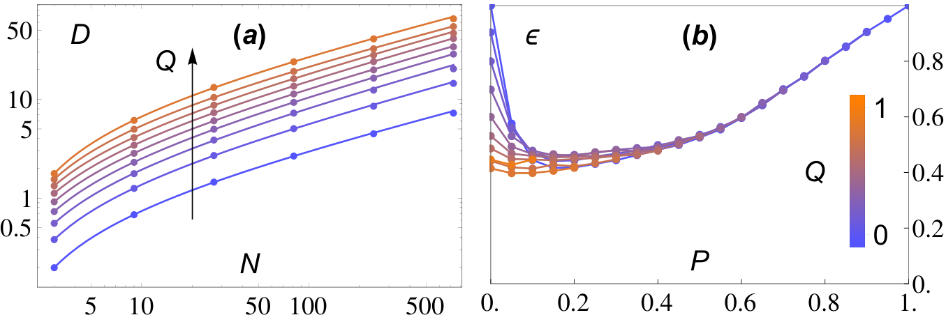
The network diameter is shown in Fig. 12(a) as a function of the number of vertices for fixed deposition probability . Full lines are power-law fits to the numerical data. The power-law behaviour of is clear from Fig. 12(b). Lines are only shown for visualisation purposes.
References
- Barabási and Stanley (1995) A.-L. Barabási and H. E. Stanley, Fractal Concepts in Surface Growth (Cambridge University Press, 1995).
- Family and Vicsek (1985) F. Family and T. Vicsek, J. Phys. A: Math. Gen. 18, L75 (1985).
- Family (1986) F. Family, J. Phys. A: Math. Gen. 19, L441 (1986).
- Meakin et al. (1986) P. Meakin, P. Ramanlal, L. M. Sander, and R. C. Ball, Phys. Rev. A 34, 5091 (1986).
- Edwards and Wilkinson (1982) S. F. Edwards and D. R. Wilkinson, Proc. R. Soc. A 381, 17 (1982).
- Vvedensky et al. (1993) D. D. Vvedensky, A. Zangwill, C. N. Luse, and M. R. Wilby, Phys. Rev. E 48, 852 (1993).
- Buceta et al. (2014) R. C. Buceta, D. Hansmann, and B. von Haeften, J. Stat. Mech.: Theory Exp. 2014 (12), P12028.
- Kardar et al. (1986) M. Kardar, G. Parisi, and Y.-C. Zhang, Phys. Rev. Lett. 56, 889 (1986).
- Bertini and Giacomin (1997) L. Bertini and G. Giacomin, Commun. Math. Phys. 183, 571 (1997).
- Gomes-Filho et al. (2021) M. S. Gomes-Filho, A. L. Penna, and F. A. Oliveira, Results Phys. 26, 104435 (2021).
- Indekeu and Fleerackers (1998) J. O. Indekeu and G. Fleerackers, Physica A 261, 294 (1998).
- Cheng et al. (1987) Z. Cheng, L. Jacobs, D. Kessler, and R. Savit, J. Phys. A: Math. Gen. 20, L1095 (1987).
- Baiod et al. (1988) R. Baiod, D. Kessler, P. Ramanlal, L. Sander, and R. Savit, Phys. Rev. A 38, 3672 (1988).
- Krug and Meakin (1991) J. Krug and P. Meakin, Phys. Rev. A 43, 900 (1991).
- Zhang (1990) Y.-C. Zhang, Physica A 170, 1 (1990).
- Hosseinabadi and Masoudi (2019) S. Hosseinabadi and A. A. Masoudi, Phys. Rev. E 99, 012130 (2019).
- Pioli et al. (2019) L. Pioli, C. Bonadonna, and M. Pistolesi, Sci. Rep. 9, 10006 (2019).
- Brykina and Egorova (2021) I. G. Brykina and L. A. Egorova, Adv. Astron. 2021, 9914717 (2021).
- Finn et al. (1982) J. E. Finn, S. Agarwal, A. Bujak, J. Chuang, L. J. Gutay, A. S. Hirsch, R. W. Minich, N. T. Porile, R. P. Scharenberg, B. C. Stringfellow, and F. Turkot, Phys. Rev. Lett. 49, 1321 (1982).
- Turcotte (1986) D. L. Turcotte, Geophys. Res. Solid Earth 91, 1921 (1986).
- Posazhennikova and Indekeu (2000) A. Posazhennikova and J. O. Indekeu, Mod. Phys. Lett. B 14, 119 (2000).
- Posazhennikova and Indekeu (2001) A. Posazhennikova and J. O. Indekeu, Int. J. Thermophys. 22, 1123 (2001).
- Indekeu et al. (2000) J. Indekeu, G. Fleerackers, A. Posazhennikova, and E. Bervoets, Physica A 285, 135 (2000).
- Posazhennikova and Indekeu (2014) A. Posazhennikova and J. O. Indekeu, Physica A 414, 240 (2014).
- Indekeu and Giuraniuc (2004) J. Indekeu and C. Giuraniuc, Physica A 336, 14 (2004).
- Indekeu and Sznajd-Weron (2003) J. O. Indekeu and K. Sznajd-Weron, Phys. Rev. E 68, 061904 (2003).
- Berx et al. (2021) J. Berx, E. Bervoets, C. V. Giuraniuc, and J. O. Indekeu, Physica A 574, 125998 (2021).
- Lacasa et al. (2008) L. Lacasa, B. Luque, F. Ballesteros, J. Luque, and J. C. Nuño, PNAS 105, 4972 (2008).
- Kaki et al. (2022) B. Kaki, N. Farhang, and H. Safari, Sci. Rep. 12, 16835 (2022).
- Yu et al. (2012) Z. G. Yu, V. Anh, R. Eastes, and D.-L. Wang, Nonlinear Process. Geophys. 19, 657 (2012).
- Ahmadlou et al. (2010) M. Ahmadlou, H. Adeli, and A. Adeli, J. Neural Transm. 117, 1099 (2010).
- Juniper and Sujith (2018) M. Juniper and R. Sujith, Annu. Rev. Fluid Mech. 50, 661 (2018).
- Paiva et al. (2022) L. R. Paiva, S. G. Alves, L. Lacasa, O. DeSouza, and O. Miramontes, arXiv:2204.11690 (2022).
- Lacasa et al. (2012) L. Lacasa, A. Nuñez, É. Roldán, J. M. R. Parrondo, and B. Luque, EPJ B 85, 217 (2012).
- Wang et al. (2018) M. Wang, A. L. M. Vilela, R. Du, L. Zhao, G. Dong, L. Tian, and H. E. Stanley, Sci. Rep. 8, 5130 (2018).
- Lacasa et al. (2015) L. Lacasa, V. Nicosia, and V. Latora, Sci. Rep. 5, 15508 (2015).
- Nuñez et al. (2012) A. M. Nuñez, L. Lacasa, J. P. Gomez, and B. Luque, in New Frontiers in Graph Theory, edited by Y. Zhang (IntechOpen, Rijeka, 2012) Chap. 6.
- Luque et al. (2009) B. Luque, L. Lacasa, F. Ballesteros, and J. Luque, Phys. Rev. E 80, 046103 (2009).
- Brú et al. (2014) A. Brú, E. Alós, J. C. Nuño, and M. F. de Dios, Sci. Rep. 4, 7550 (2014).
- Kartha (2017) M. J. Kartha, Phys. Lett. A 381, 556 (2017).
- Allouche and Shallit (2003) J.-P. Allouche and J. Shallit, Automatic Sequences: Theory, Applications, Generalizations (Cambridge University Press, 2003).
- Barabási et al. (2001) A.-L. Barabási, E. Ravasz, and T. Vicsek, Physica A 299, 559 (2001).
- Iguchi and Yamada (2005) K. Iguchi and H. Yamada, Phys. Rev. E 71, 036144 (2005).
- Song et al. (2006) C. Song, S. Havlin, and H. A. Makse, Nat. Phys. 2, 275 (2006).
- Ravasz et al. (2002) E. Ravasz, A. L. Somera, D. A. Mongru, Z. N. Oltvai, and A.-L. Barabási, Science 297, 1551 (2002).
- Dorogovtsev et al. (2002) S. N. Dorogovtsev, A. V. Goltsev, and J. F. F. Mendes, Phys. Rev. E 65, 066122 (2002).
- Donner and Donges (2012) R. V. Donner and J. F. Donges, Acta Geophys. 60, 589 (2012).
- Flanagan et al. (2019) R. Flanagan, L. Lacasa, and V. Nicosia, J. Phys. A: Math. Theor. 53, 025702 (2019).
- Goh et al. (2001) K.-I. Goh, B. Kahng, and D. Kim, Phys. Rev. E 64, 051903 (2001).
- Kim and Wilhelm (2008) J. Kim and T. Wilhelm, Physica A 387, 2637 (2008).
- Fioriti et al. (2012) V. Fioriti, A. Tofani, and A. D. Pietro, Complex Syst. 21 (2012).
- Lacasa (2016) L. Lacasa, J. Phys. A: Math. Theor. 49, 35LT01 (2016).
- de la Torre et al. (2000) A. C. de la Torre, A. Maltz, H. O. Mártin, P. Catuogno, and I. García-Mata, Phys. Rev. E 62, 7748 (2000).
- Lacasa et al. (2009) L. Lacasa, B. Luque, J. Luque, and J. C. Nuño, EPL 86, 30001 (2009).
- Gutin et al. (2011) G. Gutin, T. Mansour, and S. Severini, Physica A 390, 2421 (2011).
- Das Sarma et al. (1996) S. Das Sarma, C. J. Lanczycki, R. Kotlyar, and S. V. Ghaisas, Phys. Rev. E 53, 359 (1996).
- López et al. (1997) J. M. López, M. A. Rodríguez, and R. Cuerno, Phys. Rev. E 56, 3993 (1997).
- Giuraniuc (2006) C. V. Giuraniuc, Deposition and network models in statistical and condensed matter physics with interdisciplinary applications, Ph.D. thesis, KU Leuven (2006).
- Clauset et al. (2009) A. Clauset, C. R. Shalizi, and M. E. J. Newman, SIAM Review 51, 661 (2009).
- Olver et al. (2010) F. Olver, D. Lozier, R. Boisvert, and C. Clark, The NIST Handbook of Mathematical Functions (Cambridge University Press, New York, NY, 2010).
- Cormen et al. (2001) T. Cormen, C. Leiserson, M. Press, R. Rivest, C. Stein, and M.-H. P. Company, Introduction To Algorithms, Introduction to Algorithms (MIT Press, 2001).
- Mandelbrot et al. (2002) B. Mandelbrot, F. Damerau, M. Frame, K. McCamy, J. Van Ness, and J. Wallis, Gaussian Self-Affinity and Fractals: Globality, The Earth, 1/f Noise, and R/S, Selecta (Old or New), Volume H (Springer, 2002).
- Chen et al. (2017) L. Chen, K. E. Bassler, J. L. McCauley, and G. H. Gunaratne, Phys. Rev. E 95, 042141 (2017).