Ultimate Speed Limits to the Growth of Operator Complexity

In parallel with the study of QSL, quantifying the complexity of a physical process is a central task for the advancement of fundamental physics and quantum technologies. Lloyd pointed out that the computational complexity of physical processes is limited by QSL Lloyd 2002. Analogously, the circuit complexity of a quantum state Susskind 2016, defined as the number of elementary operations required to generate it from a reference state, can be characterized in terms of conventional QSL Brown et al. 2016a; Brown et al. 2016b; Chapman et al. 2018; Molina-Vilaplana and del Campo 2018. A complementary approach for many-body quantum systems focuses on the buildup of complexity in the time-evolution of an initial local observable, known as operator growth von Keyserlingk et al. 2018; Khemani et al. 2018; Nahum et al. 2018; Gopalakrishnan et al. 2018; Rakovszky et al. 2018. The intuition is that simple operators unitarily evolve into increasingly complex ones. Quantum information initially encoded in a few degrees of freedom is thus scrambled over the system in the course of evolution, making it impossible to recover it through local measurements and giving rise to thermalization. The unambiguous description of this scrambling process remains an open problem. One possibility is to probe it via an out-of-time-ordered correlator Larkin and Ovchinnikov 1969; Maldacena et al. 2016 that may be used to identify an analog of the Lyapunov exponent, providing a connection with classical chaos, e.g., the butterfly effect. Such quantum Lyapunov exponent obeys a universal upper bound Maldacena et al. 2016, which helps refine the notion of maximal chaos, is saturated by black holes, and is further tied to the eigenstate thermalization hypothesis Murthy and Srednicki 2019; Srednicki 1994. A related approach, which we shall pursue in this work, is to study the dynamical evolution of operators in Krylov space, exploited in numerical techniques such as the recursion method Viswanath and Müller 1994. In this context, operator growth is quantified by the so-called Krylov complexity, a measure of the delocalization of the time-dependent operator in the Krylov basis Parker et al. 2019; Barbón et al. 2019; Rabinovici et al. 2021; Dymarsky and Gorsky 2020; Jian et al. 2021. The authors of Parker et al. 2019 made a conjecture on the universal operator growth, namely, that Krylov complexity can grow at most exponentially, and it does so in generic non-integrable systems. Remarkably, its growth rate upper bounds the Lyapunov exponent, establishing a connection with the bound on out-of-time-ordered correlators Maldacena et al. 2016; Avdoshkin and Dymarsky 2020. Further studies have shown that exponential operator growth is possible in free and integrable systems Dymarsky and Smolkin 2021, while the role of the interaction graph in a quantum network has been explored in Kim et al. 2022.

Here, we characterize the growth of Krylov complexity by deriving a fundamental limit on its rate of change and by studying analytically the conditions under which this bound is saturated. Our results show that saturation, which is also found to correspond to a particular notion of minimum uncertainty, occurs whenever the dynamical evolution of the system has the underlying structure of a three-dimensional complexity algebra, which was introduced by Caputa et al. 2021. In this setting, the unitary evolution of an operator can be represented as the displacement of generalized coherent states Caputa et al. 2021, which display classical-like behavior Perelomov 1986. As demonstrated in several paradigmatic examples, the saturation of the growth rate may be possible in some chaotic systems, but quantum chaos is not required for it.

Results and Discussion
Quantum dynamics in Krylov space
Consider an isolated quantum system in which the time evolution of an observable $\mathcal{O}$ is generated by a time-independent Hamiltonian $H$ according to the Heisenberg equation of motion $\partial_{t}\mathcal{O}(t)=i[H,\mathcal{O}(t)]$, setting $\hbar=1$. The solution to this equation with the initial condition $\mathcal{O}(0)=\mathcal{O}$ is given by $\mathcal{O}(t)=e^{itH}\mathcal{O}e^{-itH}$. In terms of the Liouvillian superoperator given by $\mathcal{L}=[H,\cdot]$, the Taylor expansion of the time-evolving observable $\mathcal{O}(t)=\sum_{n=0}^{\infty}\frac{(it)^{n}}{n!}\mathcal{L}^{n}\mathcal{O}$ shows that its dynamics is contained in the complex linear span of the operators $\{\mathcal{L}^{n}\mathcal{O}\}_{n=0}^{\infty}$. This span is completely determined by the Hamiltonian and the initial observable and is known as the Krylov space.

From now on, we consider the restriction of each operator and superoperator to the Krylov space. To highlight the vector space structure, we make use of the braket notation $|A)$ when expressing an operator $A$ in an equation. We choose to equip the Krylov space with an inner product satisfying the properties

1. 1.

   $(A|\mathcal{L}B)=(\mathcal{L}A|B)$, $\forall A,B$.

2. 2.

   $(A|\mathcal{L}A)=0$, when $A$ is Hermitian.

An example of a family of inner products satisfying these two properties is given by $(A|B)=\langle e^{\beta H/2}A^{\dagger}e^{-\beta H/2}B\rangle_{\beta}$. The bracket $\langle\cdot\rangle_{\beta}$ denotes the thermal expectation value with respect to the equilibrium Gibbs state $e^{-\beta H}/Z$ and thus $(A|B)$ reduces to the Hilbert–Schmidt inner product when $\beta=0$, up to a normalization factor. It follows from the second property of the inner product that the operators $\mathcal{O}$ and $\mathcal{L}\mathcal{O}$ are orthogonal. Let $b_{0}=\norm{\mathcal{O}}$ and $b_{1}=\norm{\L\mathcal{O}}$, where $\norm{\cdot}$ is the norm induced by the inner product. By starting from the normalized vectors $\mathcal{O}_{0}=\mathcal{O}/b_{0}$ and $\mathcal{O}_{1}=\mathcal{L}\mathcal{O}/b_{1}$, we can construct an orthonormal basis $\{\mathcal{O}_{n}\}_{n=0}^{D-1}$ for the Krylov space by applying the Lanczos algorithm. This algorithm works as follows: given the first $n+1$ basis vectors, one constructs the orthogonal vector $|A_{n+1})=\mathcal{L}|\mathcal{O}_{n})-b_{n}|\mathcal{O}_{n-1})$, where $b_{n}=\norm{A_n}$ and then normalize it to obtain $|\mathcal{O}_{n+1})$. We call the constructed basis the Krylov basis. It is possible that the Krylov dimension $D$ is infinite, in which case the Lanczos algorithm never halts. We remark that the Lanczos algorithm is only guaranteed to construct an orthonormal basis if the Liouvillian is self-adjoint, i.e., the first property of the inner product is satisfied. Generally, the Lanczos algorithm involves a third term on the right-hand side of the equation for $|A_{n+1})$. This term is however always zero whenever the second property of the inner-product is satisfied. Thus, with our chosen inner-product, the action of the Liouvillian on the Krylov basis takes the specific form $\mathcal{L}|\mathcal{O}_{n})=b_{n+1}|\mathcal{O}_{n+1})+b_{n}|\mathcal{O}_{n-1})$. As pointed out in Caputa et al. 2021, this motivates one to consider abstract raising and lowering operators that we denote by $\mathcal{L}_{+}$ and $\mathcal{L}_{-}$, respectively. Their action on the Krylov basis is given by $\mathcal{L}_{+}|\mathcal{O}_{n})=b_{n+1}|\mathcal{O}_{n+1})$ and $\mathcal{L}_{-}|\mathcal{O}_{n})=b_{n}|\mathcal{O}_{n-1})$. The Liouvillian can then be expressed as their sum.

It is further convenient to introduce the real valued functions $\varphi_{n}(t)$, which appear in the expansion of $\mathcal{O}(t)$ as $|\mathcal{O}(t))=\frac{1}{\norm{\mathcal{O}}}\sum_{n=0}^{D-1}i^{n}\varphi_{n}(t)|\mathcal{O}_{n})$. We will refer to these functions as the amplitudes of the observable. These amplitudes evolve according to the recursion relation $\partial_{t}\varphi_{n}(t)=b_{n}\varphi_{n-1}(t)-b_{n+1}\varphi_{n+1}(t)$ with the initial conditions $\varphi_{0}(0)=1$ and $\varphi_{n}(0)=0$ for $n>0$. Thinking of the Krylov basis vectors as forming the sites of a one dimensional lattice, $b_{n}$ can be interpreted as a hopping amplitude, see, e.g., Parker et al. 2019; Barbón et al. 2019. In this sense, one can think of $\mathcal{O}$ as a one dimensional discrete wave function that is initially localized and then spreads out over the lattice as time evolves. An increase in the population of the sites further away from the origin reflects a greater increase of complexity of the observable. In order to quantify this, it is natural to consider the Krylov complexity of $\mathcal{O}(t)$, defined to be

The main task of our work is to bound the growth of Krylov complexity. Due to unitary dynamics, the norm of the evolution is preserved and the Krylov complexity is unchanged if one normalizes the operators studied. We will, therefore, without loss of generality, consider $\mathcal{O}$ to be normalized. By introducing the complexity operator $\mathcal{K}=\sum_{n=0}^{D-1}n|\mathcal{O}_{n})(\mathcal{O}_{n}|$, which plays the role of the position operator in the Krylov lattice, it is possible to express Krylov complexity as the “expectation value” of $\mathcal{K}$ with respect to $\mathcal{O}(t)$. More precisely, if $\langle\mathcal{K}\rangle_{t}\equiv(\mathcal{O}(t)|\mathcal{K}\mathcal{O}(t))$ then $K(t)=\langle\mathcal{K}\rangle_{t}$.

It is not self-evident that saturation of the dispersion bound can be achieved under unitary dynamics of the observable. There are very specific relations between $\mathcal{L}$, $\mathcal{O}$ and $\mathcal{K}$ that need to hold: the Liouvillian is required to be tridiagonal in the eigenbasis of the complexity operator and the initial state of the observable is required to be parallel to the eigenvector with the lowest eigenvalue. The conditions for the saturation of the dispersion bound are thus highly constrained and differ from those known for saturation of a Robertson uncertainty relation in general. The required conditions admit a geometrical interpretation, elaborated in Methods. The bound is saturated if and only if the evolution curve moves along the gradient of the Krylov complexity. This requires that the dynamics is directed along the direction that maximizes the local growth of complexity; see Methods. The only exception involves extremal points in which any direction away from the extremal point leads to saturation. This is indeed the case for $t=0$. Indeed, there exists Liouvillians of the form $\mathcal{L}=\mathcal{L}_{+}+\mathcal{L}_{-}$ for which the tangent of the generated path will be parallel with the gradient for all times.

Given this algebra, the evolving observable can be interpreted as a curve of generalized coherent states evolving according to the displacement operator $D(\xi)=e^{\xi\mathcal{L}_{+}-\overline{\xi}\mathcal{L}_{-}}$, where $\xi=it$. Moreover, the initial state is the highest weight state of the representation, which is annihilated by $\mathcal{L_{-}}$ by construction. Coherent states can be viewed as the states closest to the classical ones in the sense that they typically minimize an uncertainty relation. It is for example known that coherent states of the Harmonic oscillator saturate the Robertson uncertainty relation for the pair of observables of position and momentum. Building on this intuition, we could expect that the dispersion bound is saturated for the simplicity hypothesis. It turns out that this intuition is indeed correct. In fact, as we show in Supplementary Note 2, the dispersion bound is saturated if and only if the simplicity hypothesis holds. The saturation of the dispersion bound dictates the evolution of the Krylov complexity, where three different scenarios are possible, as shown in Figure 1a. The growth of complexity at the speed limit is described by the differential equation

with the conditions that $K(0)=0$ and $K(-t)=K(t)$. For finite Krylov dimension, saturation of the dispersion bound sets the complexity growing according to $K(t)=(D-1)\sin^{2}{\omega t}$, where $\omega=\sqrt{\frac{\gamma}{2(D-1)}}$. In this, case, the corresponding complexity algebra (3) reduces to the $\textrm{SU}(2)$ algebra. By contrast, for infinite Krylov dimension there are two distinct scenarios for the complexity growth: for $\alpha>0$ one finds $K(t)=\frac{2\gamma}{\alpha}\sinh^{2}{\frac{\sqrt{\alpha}t}{2}}$, while for $\alpha=0$ the solution reads $K(t)=\frac{\gamma}{2}t^{2}$. The complexity algebra in these two cases reduces to $\textrm{SL}(2,\mathbb{R})$ and the Heisenberg-Weyl algebra (HW), respectively. Reference examples maximizing the Krylov-complexity growth rate at all times are discussed in Supplementary Note 1. One such example with $\alpha>1$ is the Sachdev-Ye-Kitaev (SYK) model Sachdev and Ye 1993, a paradigm of quantum chaos. However, the saturation of the bound does not require quantum chaos and can indeed be achieved by a single qubit, with $\alpha=0$ (Supplementary Note 1). Together with the time-dependence of $K(t)$ and the complexity algebra, the value of $\alpha$ also determines the growth of the Lanczos coefficients in the Krylov lattice. As proven in Supplementary Note 2, the dispersion bound is saturated if and only if the Lanczos coefficients grow according to

exhibiting three different scalings as function of $\alpha$, see Figure 1b. That the simplicity hypothesis implies (5) has already been pointed out in Caputa et al. 2021. For $\alpha>1$ and large $n$, this dependence captures the linear growth $b_{n}=\sqrt{\alpha}n$ conjectured by Parker et al. to hold in generic non-integrable systems, maximizing the Krylov complexity growth Parker et al. 2019.

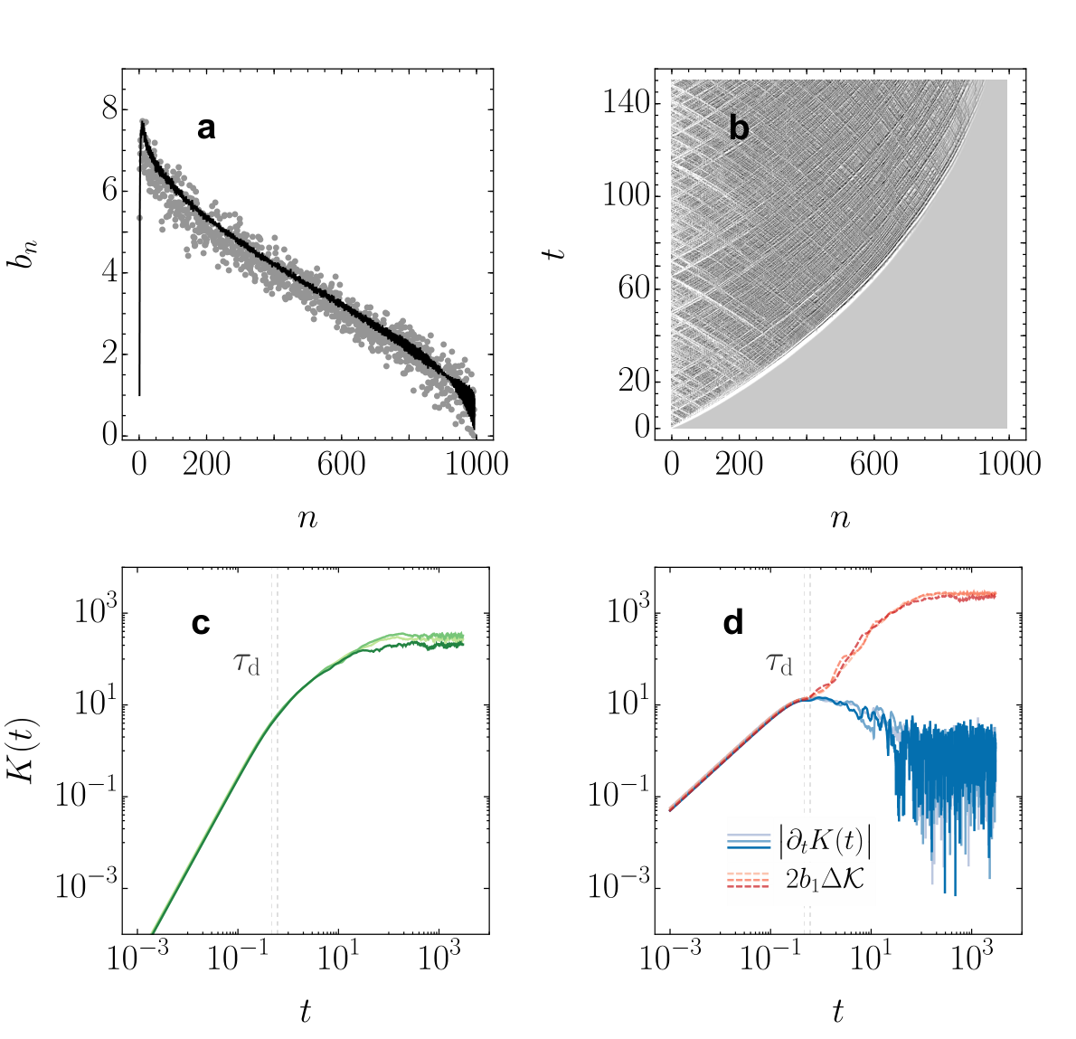
To get an understanding of the complexity growth in a generic setting, we next illustrate the Krylov dynamics of a system described by a random matrix Hamiltonian. Specifically, we consider the Krylov complexity of an ensemble $\mathcal{E}(H)$ of random matrix Hamiltonians, a paradigm of quantum chaos Haake 2010. We sample the Hamiltonian matrices $H$ from the Gaussian Orthogonal Ensemble $\mathrm{GOE}(d)$, where $d$ is the dimension of the Hilbert space. We then calculate the Lanczos coefficients $\{b_{n}\}$ with partial re-orthogonalization Simon 1984; Rabinovici et al. 2021. Specifically, we consider samples of real matrices $H=(X+X^{\intercal})/2$, where all elements $x\in\mathbb{R}$ of $X$ are pseudo-randomly generated with probability measure given by the normal distribution, $\exp( -x^2/ \big(2 \sigma^2\big))/(\sigma\sqrt{2\pi})$. In order to study the general behaviour of Lanczos coefficients, we choose an initial observable which is represented as the normalized vector $|\mathcal{O})=(1/d,1/d,\dots,1/d)^{T}$, expressed in a fixed eigenbasis of the Liouvillian. However, the following results do not depend strongly on the choice of $\mathcal{O}$, provided it is dense in the eigenbasis of the Hamiltonian. Figure 2a shows the squares of the Lanczos coefficients for a single realization and the average $\langle\{b_{n}\}\rangle_{\mathcal{E}(H)}$ over $100$ different Hamiltonians of dimension $d=32$, sampled from $\mathrm{GOE}(d)$ with standard deviation $\sigma=1$. Operator growth is displayed by the time-dependent amplitudes, which are found by solving the recursion relation and exhibit diffusion-like dynamics on the Krylov basis, shown for a single realization in Figure 2b. The corresponding time evolution of Krylov complexity and its growth rate are shown in panels c and d, respectively. Hamiltonians sampled from GOE($d$) behave as a generic system, given that the Lanczos coefficients do not, in general, grow according to (5) as shown in Figure 2a. As a result, the growth rate starts deviating from the dispersion bound around the time scale $\tau_{\text{d}}$ in Eq. (6), indicated by the vertical line in Figure 2, panels c and d. In short, while GOE Hamiltonians provide a useful paradigm in the description of quantum chaotic systems, the dynamics generated by them does not maximize the growth of Krylov complexity for $t>\tau_{\text{d}}$.

Our results establish the ultimate speed limit to operator growth in isolated quantum systems. Specifically, the dispersion bound governs the growth rate of Krylov complexity, playing the role of a Mandelstam-Tamm uncertainty relation in operator space. This bound is saturated by quantum systems in which the Liouvillian governing the time evolution fulfills a simplicity algebra. The latter arises naturally in certain quantum chaotic systems, such as the SYK model. However, other paradigmatic instances of quantum chaos, such as random-matrix Hamiltonians, do not maximize the growth of Krylov complexity. Indeed, saturation of the bound does not require quantum chaos and can be achieved, e.g., by a single qubit.

Moreover, from Eq. (8) we immediately obtain the relation between the anticommutator $[\mathcal{K},\mathcal{L}]$ and the complexity rate $\partial_{t}K$:

Therefore, the Schrödinger uncertainty relation  (7) can be recast as the dispersion bound (2) on the growth of Krylov complexity:

The Krylov space is isomorphic to a $2D$-dimensional real vector space and we can therefore consider the Euclidean metric $g$, given by the real part of the inner product. The evolution curve of $\mathcal{O}$ will then be restricted to the unit sphere of the Krylov space. This unit sphere forms a Riemannian manifold and we can consider the Krylov complexity as a function on this manifold defined by $K(\mathcal{A})=(\mathcal{A}|\mathcal{K}\mathcal{A}),$ for any element $|\mathcal{A})$ in the Krylov space with unit norm. In this sense, when we write $K(t)$ we simply mean $K(\mathcal{O}(t))$ which is consistent with how we defined complexity for the evolution. The differential of Krylov complexity will be denoted by $dK$ and its action on any tangent vector $\dot{\mathcal{A}}$ at $\mathcal{A}$ is given by $dK(\dot{\mathcal{A}})=(\dot{\mathcal{A}}|\mathcal{A})+(\mathcal{A}|\dot{\mathcal{A}})$. This differential together with the metric can be used to define the gradient of Krylov complexity. It follows from the theory of differential geometry that the gradient of Krylov complexity at $\mathcal{A}$, denoted by $\nabla K(\mathcal{A})$, is the unique vector satisfying the expression $g(\nabla K(\mathcal{A}),\dot{\mathcal{A}})=dK(\dot{\mathcal{A}})$ for all tangent vectors $\dot{\mathcal{A}}$ at $\mathcal{A}$ Lee 2018. It can be checked that the gradient must then be given by $\nabla K(\mathcal{A})=2(\mathcal{K}-\langle\mathcal{K}\rangle)\mathcal{A}$, which indeed is tangent to the unit sphere at $\mathcal{A}$. The change of Krylov complexity along the curve $\mathcal{O}(t)$, generated by the Liouvillian, is given by $\partial_{t}K(t)=g(\nabla K(t),\partial_{t}\mathcal{O}(t))$, where $\nabla K(t)$ is the gradient at $\mathcal{O}(t)$. Applying the Cauchy-Schwarz inequality on the right-hand side gives us the inequality

The right-hand side of this inequality is exactly $2b_{1}\Delta\mathcal{K}$ and we note that it is saturated if and only if the tangent vector of $\mathcal{O}(t)$ is parallel to the gradient of Krylov complexity. We also note that the gradient is the zero vector at time zero and so the dispersion bound is always initially saturated.

The unitary orbit of $\mathcal{O}$ is the set of all points $U^{\dagger}\mathcal{O}U$, where $U$ is a unitary operator. We emphasize that this is a proper subset of the unit sphere in Krylov space which, in contrast, is the set of all points $\mathcal{U}\mathcal{O}$, where $\mathcal{U}$ is a unitary superoperator. The gradient we have considered is with respect to the unit sphere and it is therefore not obvious that this gradient will ever be tangential to the unitary orbit of $\mathcal{O}$. However, the gradient is indeed tangential to the unitary orbit at time zero and at all times provided the simplicity algebra is fulfilled.

References

- Mandelstam and Tamm (1945) L. Mandelstam and I. Tamm, J. Phys. USSR 9, 249 (1945).
- Margolus and Levitin (1998) N. Margolus and L. B. Levitin, Physica D: Nonlinear Phenomena 120, 188 (1998).
- Pires et al. (2016) D. P. Pires, M. Cianciaruso, L. C. Céleri, G. Adesso, and D. O. Soares-Pinto, Phys. Rev. X 6, 021031 (2016).
- Campaioli et al. (2018) F. Campaioli, F. A. Pollock, F. C. Binder, and K. Modi, Phys. Rev. Lett. 120, 060409 (2018).
- Taddei et al. (2013) M. M. Taddei, B. M. Escher, L. Davidovich, and R. L. de Matos Filho, Phys. Rev. Lett. 110, 050402 (2013).
- del Campo et al. (2013) A. del Campo, I. L. Egusquiza, M. B. Plenio, and S. F. Huelga, Phys. Rev. Lett. 110, 050403 (2013).
- Deffner and Lutz (2013) S. Deffner and E. Lutz, Phys. Rev. Lett. 111, 010402 (2013).
- Campaioli et al. (2019) F. Campaioli, F. A. Pollock, and K. Modi, Quantum 3, 168 (2019).
- Shanahan et al. (2018) B. Shanahan, A. Chenu, N. Margolus, and A. del Campo, Phys. Rev. Lett. 120, 070401 (2018).
- Okuyama and Ohzeki (2018) M. Okuyama and M. Ohzeki, Phys. Rev. Lett. 120, 070402 (2018).
- Lloyd (2000) S. Lloyd, Nature 406, 1047 (2000).
- Bukov et al. (2019) M. Bukov, D. Sels, and A. Polkovnikov, Phys. Rev. X 9, 011034 (2019).
- Caneva et al. (2009) T. Caneva, M. Murphy, T. Calarco, R. Fazio, S. Montangero, V. Giovannetti, and G. E. Santoro, Phys. Rev. Lett. 103, 240501 (2009).
- Giovannetti et al. (2011) V. Giovannetti, S. Lloyd, and L. Maccone, Nature Photonics 5, 222 (2011).
- Eisert et al. (2015) J. Eisert, M. Friesdorf, and C. Gogolin, Nature Physics 11, 124 (2015).
- Nicholson et al. (2020) S. B. Nicholson, L. P. García-Pintos, A. del Campo, and J. R. Green, Nature Physics 16, 1211 (2020).
- Braunstein et al. (1996) S. L. Braunstein, C. M. Caves, and G. Milburn, Annals of Physics 247, 135 (1996).
- Lloyd (2002) S. Lloyd, Phys. Rev. Lett. 88, 237901 (2002).
- Susskind (2016) L. Susskind, Fortschritte der Physik 64, 24 (2016).
- Brown et al. (2016a) A. R. Brown, D. A. Roberts, L. Susskind, B. Swingle, and Y. Zhao, Phys. Rev. Lett. 116, 191301 (2016a).
- Brown et al. (2016b) A. R. Brown, D. A. Roberts, L. Susskind, B. Swingle, and Y. Zhao, Phys. Rev. D 93, 086006 (2016b).
- Chapman et al. (2018) S. Chapman, M. P. Heller, H. Marrochio, and F. Pastawski, Phys. Rev. Lett. 120, 121602 (2018).
- Molina-Vilaplana and del Campo (2018) J. Molina-Vilaplana and A. del Campo, Journal of High Energy Physics 2018, 12 (2018).
- von Keyserlingk et al. (2018) C. W. von Keyserlingk, T. Rakovszky, F. Pollmann, and S. L. Sondhi, Phys. Rev. X 8, 021013 (2018).
- Khemani et al. (2018) V. Khemani, A. Vishwanath, and D. A. Huse, Phys. Rev. X 8, 031057 (2018).
- Nahum et al. (2018) A. Nahum, S. Vijay, and J. Haah, Phys. Rev. X 8, 021014 (2018).
- Gopalakrishnan et al. (2018) S. Gopalakrishnan, D. A. Huse, V. Khemani, and R. Vasseur, Phys. Rev. B 98, 220303 (2018).
- Rakovszky et al. (2018) T. Rakovszky, F. Pollmann, and C. W. von Keyserlingk, Phys. Rev. X 8, 031058 (2018).
- Larkin and Ovchinnikov (1969) A. I. Larkin and Y. N. Ovchinnikov, Soviet Journal of Experimental and Theoretical Physics 28, 1200 (1969).
- Maldacena et al. (2016) J. Maldacena, S. H. Shenker, and D. Stanford, Journal of High Energy Physics 2016, 106 (2016).
- Murthy and Srednicki (2019) C. Murthy and M. Srednicki, Phys. Rev. Lett. 123, 230606 (2019).
- Srednicki (1994) M. Srednicki, Physical Review E 50 (1994).
- Viswanath and Müller (1994) V. S. Viswanath and G. Müller, The Recursion Method, Vol. Lecture Notes in Physics (Springer, 1994).
- Parker et al. (2019) D. E. Parker, X. Cao, A. Avdoshkin, T. Scaffidi, and E. Altman, Phys. Rev. X 9, 041017 (2019).
- Barbón et al. (2019) J. Barbón, E. Rabinovici, R. Shir, and R. Sinha, J. High Energ. Phys. 2019, 264 (2019).
- Rabinovici et al. (2021) E. Rabinovici, A. Sánchez-Garrido, R. Shir, and J. Sonner, J. High Energ. Phys. 2021, 62 (2021).
- Dymarsky and Gorsky (2020) A. Dymarsky and A. Gorsky, Phys. Rev. B 102, 085137 (2020).
- Jian et al. (2021) S.-K. Jian, B. Swingle, and Z.-Y. Xian, Journal of High Energy Physics 2021, 14 (2021).
- Avdoshkin and Dymarsky (2020) A. Avdoshkin and A. Dymarsky, Phys. Rev. Research 2, 043234 (2020).
- Dymarsky and Smolkin (2021) A. Dymarsky and M. Smolkin, Phys. Rev. D 104, L081702 (2021).
- Kim et al. (2022) J. Kim, J. Murugan, J. Olle, and D. Rosa, Phys. Rev. A 105, L010201 (2022).
- Caputa et al. (2021) P. Caputa, J. M. Magan, and D. Patramanis, arXiv:2109.03824 (2021), arXiv: 2109.03824.
- Perelomov (1986) A. Perelomov, Generalized Coherent States and Their Application (Springer, 1986).
- Davidson (1965) E. R. Davidson, The Journal of Chemical Physics Volume 42 (1965).
- Sachdev and Ye (1993) S. Sachdev and J. Ye, Phys. Rev. Lett. 70, 3339 (1993).
- Haake (2010) F. Haake, Quantum Signatures of Chaos (Springer, Berlin, 2010).
- Simon (1984) H. Simon, Mathematics of Computation - Math. Comput. 42, 115 (1984).
- Lee (2018) J. M. Lee, Introduction to Riemannian manifolds, 2nd ed. (Springer, 2018).