Learning Latent Causal Dynamics
Supplement to: “Learning Latent Causal Dynamics”
Abstract
One critical challenge of time-series modeling is how to learn and quickly correct the model under unknown distribution shifts. In this work, we propose a principled framework, called LiLY, to first recover time-delayed latent causal variables and identify their relations from measured temporal data under different distribution shifts. The correction step is then formulated as learning the low-dimensional change factors with a few samples from the new environment, leveraging the identified causal structure. Specifically, the framework factorizes unknown distribution shifts into transition distribution changes caused by fixed dynamics and time-varying latent causal relations, and by global changes in observation. We establish the identifiability theories of nonparametric latent causal dynamics from their nonlinear mixtures under fixed dynamics and under changes. Through experiments, we show that time-delayed latent causal influences are reliably identified from observed variables under different distribution changes. By exploiting this modular representation of changes, we can efficiently learn to correct the model under unknown distribution shifts with only a few samples.
Keywords:
Nonlinear ICA, Causal discovery, Latent variable model, State space model, Representation learning1 Introduction
Unknown distribution shifts or nonstationarity in natural signals have posed a critical challenge for time-series forecasting. For example, if the distribution shifts (e.g., changing dynamics, heterogeneous noise, etc.) are not well captured, models fit on these data samples will either overfit specific kinds of changes, or learn to use only the stationary parts for prediction, both of which significantly degrade the predictive performances. One prevalent approach in the literature is to actively transfer the time-series model under the distribution shifts. However, if one is not aware of how the changes influence the underlying data generating process, one may not know how to target specific mechanisms and change the learned model efficiently. In other words, the true underlying processes or a graphical model that encode the change property of the distribution need to be given as a priori. To accomplish this step, causal discovery is often used. Causal discovery aims to identify the underlying structure of the data generation process by exploiting an appropriate class of assumptions (Spirtes et al. 1993; Pearl 2000). Although distribution changes are not desired by time-series models, these changes, serving as a “soft” way of intervention, have proved to greatly improve the identifiability results for learning the latent causal structure (Yao et al. 2021; Bengio et al. 2019; Ke et al. 2019). For this reason, a natural solution is to first exploit the distribution changes to identify the latent causal dynamics, and then use the uncovered structure to correct the model under changes.
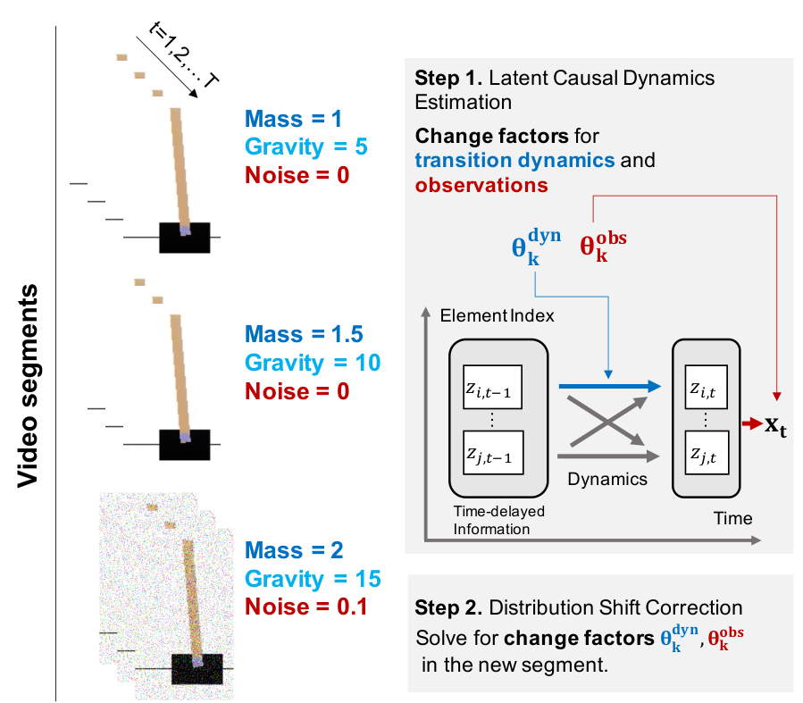
In this work, we propose a principled framework, called LiLY, to first recover time-delayed latent causal variables and identify their relations from measured temporal data under different distribution shifts. The transfer step is then formulated as learning the low-dimensional change factors with a few samples from the new environment, leveraging the identified causal structure. For instance, Fig. 1 shows an example of multiple video segments of a physical system (i.e., cartpole) under different mass, gravity and environment rendering settings. With LiLY, the differences across segments are characterized by change factors of segment that encode changes in transition dynamics, and changes in observation modeled by . We then present a generalized time-series data generative model that takes these change factors as arguments for modeling the distribution changes. Specifically, the proposed latent variable model factorizes distribution changes in fixed dynamics, time-varying transitions and observation by constructing partitioned latent subspaces. If the underlying latent causal dynamics augmented with change factors is uncovered, correcting distribution shifts can be performed efficiently by estimating the change factors in a new segment.
| Theory |
|
|
|
| ||||||||
|---|---|---|---|---|---|---|---|---|---|---|---|---|
| PCL | ✗ | ✗ | ✗ | ✓ | ||||||||
| HM-NLICA | ✗ | ✗ | ✗ | ✗ | ||||||||
| SlowVAE | ✗ | ✗ | ✗ | ✗ | ||||||||
| SNICA | ✓ | ✓ | ✗ | ✗ | ||||||||
| LEAP | ✗ | ✓ | ✗ | ✓ | ||||||||
| LiLY † | ✓ | ✓ | ✓ | ✓ |
However, estimating latent causal structure from observations is notoriously challenging because the latent variables, even with independent factors of variation (Locatello et al. 2019), are not identifiable in the most general case (Hyvärinen & Pajunen 1999). There exist several pieces of work aiming to uncover causally related latent variables under linear relations or minimality assumptions. As early as (Spearman 1928), vanishing Tetrad conditions were exploited to identify latent variables in linear-Gaussian models (Silva et al. 2006). Generalized Independent Noise (GIN) condition estimates linear, non-Gaussian latent variable causal graph (Xie et al. 2020). Recently, in the field of nonlinear Independent Component Analysis (ICA), identifiability results have been established (Hyvarinen & Morioka 2016; Hyvarinen & Morioka 2017; Hyvarinen et al. 2019; Khemakhem et al. 2020; Sorrenson et al. 2020) by using certain side information, such as class labels, in addition to independence. For time-series data, history information is widely used as side information for nonlinear ICA. However, most existing work that establishes identifiability results considers either stationary independent sources such as PCL (Hyvarinen & Morioka 2017), SlowVAE (Klindt et al. 2020) or under linear transition assumptions such as SlowVAE (Klindt et al. 2020) and SNICA (Hälvä et al. 2021), or with certain structure such as Markov properties in HM-NLICA (Hälvä & Hyvarinen 2020). LEAP (Yao et al. 2021), which is the closest work to ours, has established the identifiability of the nonparametric latent temporal processes in certain nonstationary cases, under the condition that the distribution of the noise terms of the latent processes vary across segments.
Our theory can be differentiated from the prior work in four aspects as summarized in Table 1:
- 1.
We consider a very general nonstationary case which includes changing causal dynamics such as changes in the influencing strength or switching some edges off (Li et al. 2020), nonstationary noise distributions across domains (Yao et al. 2021), and domain shifts in observation (Sahoo et al. 2021), etc., as special cases;
- 2.
We establish the identifiability results for nonparametric, causally-related time-delayed latent processes, instead of independent processes, or under linear assumptions;
- 3.
We allow both stationary and nonstationary latent processes to co-exist by using partitioned latent subspaces in the data generating processes. The identifiability results under this setting are appealing to real-world data where whether and how the distribution changes are unknown. Our identifiability condition is generally much weaker than the ones in (Yao et al. 2021) because we further benefit from distribution changes under fixed causal dynamics, while LEAP assumes all latent processes are changed across contexts.
Through experiments, we show that time-delayed latent causal processes are reliably identified from observed variables under different distribution shifts and dependency structures. By exploiting this modular representation of changes, we can efficiently learn to correct the model under unknown distribution shifts with only a few samples.
2 Related Work
2.1 Nonlinear ICA for Time Series
Temporal structure and nonstationarities were used to achieve identifiability of nonlinear ICA. Hyvarinen & Morioka 2016 proposed time-contrastive learning (TCL) based on the independent sources assumption and leverage variability in variance terms. (Hyvarinen & Morioka 2017) developed a permutation-based contrastive (PCL) learning framework which discriminates between true independent sources and permuted sources, and the model is identifiable under the uniformly dependent assumption. (Hälvä & Hyvarinen 2020) combined nonlinear ICA with a Hidden Markov Model (HMM) to automatically model nonstationarity without the need for manual data segmentation. (Khemakhem et al. 2020) introduced VAEs to approximate the true joint distribution over observed and auxiliary nonstationary regimes. The conditional distribution in their work is assumed to be within exponential families to achieve identifiability on the latent space. The most recent literature on nonlinear ICA for time-series is the work of (Yao et al. 2021), which proposed both a nonparametric condition leveraging the nonstionary noise terms, and a linear, parametric condition leveraging the functional form with generalized Laplacian properties of the noise terms.
2.2 Causal Discovery from Time Series
Inferring the causal structure from time-series data is critical to many fields including machine learning (Berzuini et al. 2012), econometrics (Ghysels et al. 2016), and neuroscience (Friston 2009). Most existing work focuses on estimating the temporal causal relations between observed variables. For this task, constraint-based methods (Entner & Hoyer 2010) apply the conditional independence tests to recover the causal structures, while score-based methods (Murphy et al. 2002; Pamfil et al. 2020) define score functions to guide a search process. Furthermore, Malinsky & Spirtes 2018; Malinsky & Spirtes 2019 propose to fuse both conditional independence tests and score-based methods. The Granger causality (Granger 1969) and its non-linear variations (Tank et al. 2018; Löwe et al. 2020) are also widely used.
3 Problem Formulation
We first present a holistic, modular time-series data generative model that factorizes distribution changes in fixed dynamics, time-varying transitions and observation by constructing partitioned latent subspaces. We then define the properties of the generative model which suffice the identifiability of time-delayed causal dynamics. Finally, we formulate the problem of distribution shift correction as learning the change factor representation in a new environment with the identified latent causal structure.
3.1 A Modular Representation of Changes
Following (Huang et al. 2020; Huang et al. 2021), we can represent the changes in a compact way by using a low-dimensional vector . Specifically, let denotes domain or segment index. Suppose there exist domains or segments, i.e., with . In each segment, we observe time series generated by an arbitrary invertible nonlinear mixture of the underlying temporal processes . We partition the latent space into three blocks where denotes the sth component of the fixed dynamics parts, denotes the cth component of the changing dynamics parts, and is the oth component of the global changes (e.g., styles). We assume the data generating process in each segment can be described by the transition function for each dimension of that takes its parent nodes change factors, and noise terms as inputs, and the mixing function as:
| (1) |
where denote the set of (time-delayed) parent nodes of , and terms are mutually independent (i.e., spatially and temporally independent) random noises in each segment. The vector embeds the information of segment . Note that with Eq. 1, we allow a very general class of changes in the model, which includes changing causal dynamics such as changes in the influencing strength or switching some edges off (Li et al. 2020), nonstationary noise distributions across segments (Yao et al. 2021), and domain shifts in observation (Sahoo et al. 2021), etc., all as special cases.
Remark 1.
The mutual independence of noise terms over space and time imply that: (1) are independent from the parent nodes , and (2) are conditional independent given the history information up to maximum time lag and segment embeddings or index.
This Remark suggests that the Independent Noise (IN) condition (Pearl et al. 2000) and Conditional Independence (CI) condition (Hyvarinen et al. 2019), both of which are common assumptions for causal discovery, are naturally satisfied in time-series data under random noise.
3.2 Identifiability of Time-Delayed Causal Dynamics
We define the identifiability of time-delayed latent causal dynamics in the representation function space. If the latent variables can be identified at least up to permutation and component-wise invertible nonlinearities, we say that latent causal dynamics are also identifiable because conditional independence relations fully characterize time-delayed causal relations in a time-delayed causally sufficient system.
Definition 1 (Identifiable Latent Causal Dynamics).
Formally let be a sequence of observed variables generated by the true temporally causal latent processes specified by given in Eq. 1. A learned generative model is observationally equivalent to if the model distribution matches the data distribution everywhere. We say latent causal processes are identifiable if observational equivalence can lead to identifiability of the latent variables up to permutation and component-wise invertible transformation :
| (2) | ||||
where is the observation space.
3.3 Distribution Shift Correction
We first assume that the latent causal dynamics model in Eq. 1 is identified (we will explain under what conditions the identifiability can be achieved in Sec. 4 and how in Sec. 5). Then correcting distribution shifts is equivalent to learning the embeddings in the new environment. In practice, distributions are often changed in a sparse or local way given the causal disentanglement, i.e, only a few factors may change simultaneously, which is known as sparse mechanism shift assumption (Schölkopf et al. 2021). Following the assumption, we encode with low-dimensional embeddings, in order to capture only the domain differences.
4 Theory
In this section, we establish the identifiability theory of nonparametric time-delayed latent causal processes under three different types of distribution shifts. W.l.o.g., we consider the latent processes with maximum time lag . In particular, (1) under fixed causal dynamics, we leverage the distribution changes for different values of ; (2) under changing causal dynamics, we exploit the changing causal influences on under different domain , and (3) under global observation changes, the nonstationarity under different values of is exploited. We illustrate through examples that, even without explicit changes in causal influences, the latent causal processes are generally identifiable if the process noises are not perfectly Gaussian. We show that the identifiability results can further benefit from nonstationarity with weaker identifiability conditions. This identifiability theory extends the prior work (Yao et al. 2021; Klindt et al. 2020; Hyvarinen & Morioka 2017) by allowing causal relations between latent factors, instead of independent sources, and partitioned subspaces with both fixed and/or changing causal influences. The proofs are provided in Appendix S1.
4.1 Identifiability under Fixed Causal Dynamics
Let . Assume that is twice differentiable in and is differentiable in , . Note that the parents of may be only a subset of ; if is not a parent of , then . Below we provide a sufficient condition for the identifiability of , followed by a discussion of specific unidentifiable and identifiable cases to illustrate how general it is.
Theorem 1 (Identifiablity under a Fixed Temporal Causal Model).
Suppose there exists invertible function that maps to , i.e.,
| (3) |
such that the components of are mutually independent conditional on . Let
| (4) | ||||
If for each value of , , as vector functions in , , …, , are linearly independent, then must be an invertible, component-wise transformation of a permuted version of .
The linear independence condition in Theorem 1 is the core condition to guarantee the identifiability of from the observed . To make this condition more intuitive, below we consider specific unidentifiable cases, in which there is no temporal dependence in or the noise terms in are additive Gaussian, and two identifiable cases, in which has additive, heterogeneous noise or follows some linear, non-Gaussian temporal process.
Let us start with two unidentifiable cases. In case , is an independent and identically distributed (i.i.d.) process, i.e., there is no causal influence from any component of to any . In this case, and (defined in Eq. 4) are always for , since does not involve . So th linear independence condition is violated. In fact, this is the regular nonlinear ICA problem with i.i.d. data, and it is well-known that the underlying independent variables are not identifiable (Hyvärinen & Pajunen 1999).
In case , all follow an additive noise model with Gaussian noise terms, i.e.,
| (5) |
where is a transformation and the components of the Gaussian vector are independent and also independent from . Then is constant, and , violating the linear independence condition. In the following proposition we give some alternative solutions and verify the unidentifiability in this case.
Proposition 1 (Unidentifiability under Gaussian Noise).
Suppose was generated by Eq. 5, where the components of are mutually independent Gaussian and also independent from . Then any , where is an arbitrary non-singular diagonal matrix, is an arbitrary orthogonal matrix, and is a diagonal matrix with as its diagonal entry, is a valid solution to satisfy the condition that the components of are mutually independent conditional on .
Roughly speaking, for a randomly chosen conditional density function in which is not independent from (i.e., there is temporal dependence in the latent processes) and which does not follow an additive noise model with Gaussian noise, the chance for its specific second- and third-order partial derivatives to be linearly dependent is slim. Now let us consider two cases in which the latent temporally processes are naturally identifiable under some technical conditions. First consider case , where follows a heterogeneous noise process, in which the noise variance depends on its parents:
| (6) |
Here we assume is standard Gaussian and are mutually independent and independent from . , which depends on , is the standard deviation of the noise in . (For conciseness, we drop the argument of and when there is no confusion.) Note that in this model, if is 0 for all , it reduces to a multiplicative noise model. The identifiability result of is established in the following proposition.
Corollary 1 (Identifiability under Heterogeneous Noise).
Let us then consider another special case, denoted by , with linear, non-Gaussian temporal model for : the latent processes follow Eq. 5, with being a linear transformation and following a particular class of non-Gaussian distributions. The following corollary shows that is identifiable as long as each receives causal influences from some components of .
Corollary 2 (Identifiability under a Specific Linear, Non-Gaussian Model for Latent Processes).
Suppose was generated according to Eq. 5, in which is a linear transformation and for each , there exists at least one such that . Assume the noise term follows a zero-mean generalized normal distribution:
| (7) |
If Eq. 3 holds, then must be an invertible, component-wise transformation of a permuted version of .
4.2 Further Benefits from Changing Causal Influences
Yao et al. 2021 established the identifiability of the latent temporal causal processes in certain nonstationary cases, under the condition that the noise term in each , relative to its parents in , changes across contexts corresponding to . Here we show that the identifiability result shown in the previous section can further benefit from nonstationarity of the causal model, and our identifiability condition is generally much weaker than that in (Yao et al. 2021): we allow changes in the noise term or causal influence on from its parents in , and our “sufficient variability” condition is just a necessary condition for that in (Yao et al. 2021) because of the additional information that one can leverage. Let be , which is defined in Eq. 4, in the context. Similarly, Let be in the context. Let
where and As provided below, in our case, the identifiablity of is guaranteed by the linear independence of the whole function vectors and , with . However, the identifiability result in (Yao et al. 2021) relies on the linear independence of only the last components of and with ; this linear independence is generally a much stronger condition.
Theorem 2 (Identifiability under Changing Causal Dynamics).
Suppose and that the conditional distribution may change across values of the context variable , denoted by , , …, . Suppose the components of are mutually independent conditional on in each context. Assume that the components of produced by Eq. 3 are also mutually independent conditional on . If the function vectors and , with , are linearly independent, then is a permuted invertible component-wise transformation of .
Theorem 3 (Identifiability under Observation Changes).
Suppose and that the conditional distribution may change across values of the context variable , denoted by , , …, . Suppose the components of are mutually independent conditional on in each context. Assume that the components of produced by Eq. 3 are also mutually independent conditional on . If the function vectors and , with , are linearly independent, then is a permuted invertible component-wise transformation of .
Corollary 3 (Identifiability under Modular Distribution Shifts).
Assume the data generating process in Eq. 1. If the three partitioned latent components respectively satisfy the conditions in Theorem 1, Theorem 2, and Theorem 3, then must be an invertible, component-wise transformation of a permuted version of .
5 LiLY: Learning Latent Causal Dynamics
Given our identifiability results, we propose Learning Latent causal dYnamics (LiLY) framework to estimate the latent causal dynamics under modular distribution shifts, by extending Sequential Variational Auto-Encoders (Li & Mandt 2018) with tailored modules to model different distribution shifts, and enforcing the conditions in Sec. 4 as constraints. We give the estimation procedure of the latent causal dynamics model in Eq. 1. The model architecture is showcased in Fig. 2. The framework has the following three major components. The implementation details are in Appendix S3.1.
Modular Prior Network
The core component of the estimation is to learn the three types of distribution changes. We leverage the partitioned estimated latent subspaces and model their distribution changes in conditional priors. In particular, for (1) fixed causal dynamics processes , their transition priors are obtained by first learning inverse transition functions that take the estimated latent variables and output random noise terms, and applying the change of variables formula to the transformation: ; (2) for changing causal dynamics, we evaluate by learning a holistic inverse dynamics that takes the estimated change factors for dynamics as inputs, and similarly for (3) observation changes , we learn to project them to invariant noise terms by which takes the change factors as arguments, and obtains as the prior. Two immediate benefits are brought by learning the inverse dynamics function: (1) compared with forward prediction, learning to recover the noise is more appealing for nonparametric processes, in the sense that using forward prediction with a fixed loss function, one cannot model latent processes without parametric forms. For example, heterogeneous noise model in the latent processes (Eq. 6) cannot be estimated by forward prediction with loss, and (2) (conditional) mutual independence of the estimated latent variables can be easily enforced by summing up all estimated component densities when obtaining the joint . Furthermore, given that the Jacobian is lower-triangular because of mutually-independent noise, we can efficiently compute its determinant as the product of diagonal terms. Learning the inverse dynamics won’t cause computational issues as well.
Factorized Inference
We infer the posteriors of each time step , using only the observation at that time step and with the change factors allocated for global changes. Recurrent inference (Yao et al. 2021) is not used because in Eq. 1, preserves all the information of the current system states so the joint probability can be factorized into into product of these terms.
Change Representation
To allow transfer in a new environment, instead of learning separate transformation or dynamics in each domain (Yao et al. 2021), we learn to embed domain index into low-dimensional change factors and insert them as inputs to the inverse dynamics function, or the encoder/decoder function, respectively. We make the best use of the multiple domains created by distribution changes, and efficiently correct distribution shits with only a few samples from the target domain, since only the low-dimensional change factors need to be re-estimated.
We train the VAE using the ELBO objective , in which we use mean-squared error (MSE) for the reconstruction likelihood , and use sampling approach to estimate the , since with a learned modular prior, KLD does not have an explicit form.
6 Experimental Results
We comparatively evaluate LiLY on a number of time-series datasets. We aim to answer the following questions:
- 1.
Does LiLY reliably learn temporally-causal latent processes from scratch under different distribution changes?
- 2.
Is history/nonstationary information necessary for the identifiability of latent causal variables?
- 3.
How do assumptions in previous nonlinear ICA (i.e., independent sources, nonstationary noises) distort the identifiability results if there are time-delayed causal relations between the latent factors, or if the nonstationary cases involve time-varying causal relations?
Evaluation Metrics
We report Mean Correlation Coefficient (MCC) on the validation dataset. MCC is a standard metric in the ICA literature for continuous variables which measure the identifiability of the learned latent causal processes. MCC is close to 1 when latent variables are identifiable up to permutation and componentwise invertible transformation in the noiseless case. To evaluate the transfer performances, we visualize the learned change factors with a few samples (16 in our experiments) from the target segment, and compare them with the true change factors.
Baselines
We used nonlinear ICA baselines: (1) BetaVAE (Higgins et al. 2016) which ignores both history and nonstationarity information; (2) iVAE (Khemakhem et al. 2020) and TCL (Hyvarinen & Morioka 2016) which leverage nonstationarity to establish identifiability but assumes independent factors, and (3) SlowVAE (Klindt et al. 2020) and PCL (Hyvarinen & Morioka 2017) which exploits temporal constraints but assumes independent sources and stationary processes, and (4) LEAP (Yao et al. 2021) which assumes nonstationary, causal processes but models all types of distribution changes in nonstationary noise.
6.1 Synthetic Experiments
We generate synthetic datasets that satisfy our identifiability conditions in the theorems following the procedures described in Appendix S2.1.1. In particular, we consider three representative simulation settings respectively to validate the identifiability results under fixed causal dynamics, changing causal dynamics, and modular distribution shift which contains fixed dynamics, changing dynamics and global changes together in the latent processes. For synthetic datasets with fixed and changing causal dynamics, we set latent size . For the modular shift dataset, we add one dimension for global observation changes. The lag number of the process is set to . The mixing function is a random three-layer MLP with LeakyReLU units.
6.1.1 Comparisons with Baselines
As presented in Table 2, our framework can recover the latent processes under fixed dynamics (heterogeneous noise model), under changing causal dynamics and under modular distribution shifts. The baselines that do not exploit history or nonstationarity cannot recover the latent processes. SlowVAE and PCL distort the results due to independent source assumptions. LEAP, although exploits both the history and nonstationarity information, considers only limited nonstationary cases in which the noise distributions are changing, thus cannot recover the causal latent processes under changing causal dynamics and modular distribution shifts.
| Simulation Setting | |||||||||
|---|---|---|---|---|---|---|---|---|---|
|
|
| |||||||
| LiLY | 0.954 ±0.009 | 0.958 ±0.017 | 0.993 ±0.001 | ||||||
| LEAP | – | 0.726 ±0.187 | 0.657 ±0.108 | ||||||
| SlowVAE | 0.411 ±0.022 | 0.511 ±0.062 | 0.406 ±0.045 | ||||||
| PCL | 0.516 ±0.043 | 0.599 ±0.041 | 0.564 ±0.049 | ||||||
| i-VAE | – | 0.581 ±0.083 | 0.557 ±0.005 | ||||||
| TCL | – | 0.399 ±0.021 | 0.297 ±0.078 | ||||||
| -VAE | 0.353 ±0.001 | 0.523 ±0.009 | 0.433 ±0.045 | ||||||


6.1.2 Fixed Causal Dynamics
We use a heterogeneous noise model in Eq. 6 with standard Gaussian noise terms as the latent processes. The transition function is a random two-layer MLP with LeakyReLU units, and the a mean function of its history . The latent dynamics is identifiable since the history modulates both the mean and variance of the transition distribution. Fig. 5 gives the results on heterogeneous noise datasets. The latent processes are successfully recovered, as indicated by high MCC for the casually-related factors. Panel (b) suggests that the latent causal variables are estimated up to permutation and componentwise invertible transformation.
6.1.3 Changing Causal Dynamics
We use a Gaussian additive noise model with changes in the influencing strength as the latent processes. It has been shown in Proposition 1 that this latent dynamics, if without changes, is unidentifiable. We use a random two-layer MLP with LeakyReLU units as the transition function. To add changes, we vary the values of the first layer of the MLP across segments. In Fig. 5, the latent processes are successfully recovered, as indicated by high MCC and the recovered latent factors, which shows the further benefits brought by distribution changes.
6.1.4 Modular Distribution Shift
To partition the latent space, we allocate six latent processes (variables) to fixed heterogeneous noise dynamics as in Sec. 6.1.2, two latent processes following changing causal dynamics in Sec. 6.1.3, and the last latent variable is sampled from Gaussian distribution whose mean and variance vary by segment index. The results for the modular shift dataset are in Fig. 5. Similarly, the latent processes are recovered, as indicated by (a) high MCC and (b) invertible mappings between the estimated and true latent variables.
6.2 Causal Discovery from Videos
We evaluate LiLY on the modified cartpole (Huang et al. 2021) video dataset and compare the performances with LEAP. Modified Cartpole is a nonlinear dynamical system with cart positions and pole angles as the true state variables. The dataset has 6 source domains with different gravity values . Together with the 2 discrete actions (i.e., left and right), we have 12 segments of data with changing causal dynamics. We fit LiLY with two-dimensional change factors . We set the latent size and the lag number . In Fig. 6, the latent causal processes are recovered, as seen from (a) high MCC for the latent causal processes; (b) the latent factors are estimated up to componentwise transformation; (c) the latent traversals confirm that the two latent causal variables correspond to the position and pole angle, and (d) our model outperforms LEAP, which only considers nonstationarity in noise distributions.

We visualize the learned change factors in panel (e). We also plot the estimated change factor in a new environment () with 16 samples over 3 random seeds. The positive association between the true and estimated change factors indicates that meaningful change representation in the source environment is learned. The mean of the estimated change factor in the target environment is aligned with the true value, showing that we can efficiently adapt with a few samples from the target environment.
7 Conclusion
We established theories for the identifiability of latent causal dynamics from their observed nonlinear mixtures under fixed dynamics and unknown distribution shifts. The main limitation of this work is that instantaneous causal influences between latent causal processes are not allowed. We acknowledge that there exist situations where the resolution is low and there appears to be instantaneous dependence. However, there are several pieces of work dealing with causal discovery from measured time series in such situations; see. e.g., (Granger 1987; Gong* et al. 2015; Danks & Plis 2013; Gong et al. 2017). Extending our theories and framework to address the issue of instantaneous dependency or instantaneous causal relations in the latent structure will be one line of our future work.
References
- Bengio et al. (2019) Bengio, Y., Deleu, T., Rahaman, N., Ke, R., Lachapelle, S., Bilaniuk, O., Goyal, A., and Pal, C. A meta-transfer objective for learning to disentangle causal mechanisms. arXiv preprint arXiv:1901.10912, 2019.
- Berzuini et al. (2012) Berzuini, C., Dawid, P., and Bernardinell, L. Causality: Statistical perspectives and applications. John Wiley & Sons, 2012.
- Danks & Plis (2013) Danks, D. and Plis, S. Learning causal structure from undersampled time series. In JMLR: Workshop and Conference Proceedings, pp. 1–10, 2013.
- Entner & Hoyer (2010) Entner, D. and Hoyer, P. O. On causal discovery from time series data using fci. Probabilistic graphical models, pp. 121–128, 2010.
- Friston (2009) Friston, K. Causal modelling and brain connectivity in functional magnetic resonance imaging. PLoS biology, 7(2):e1000033, 2009.
- Ghysels et al. (2016) Ghysels, E., Hill, J. B., and Motegi, K. Testing for granger causality with mixed frequency data. Journal of Econometrics, 192(1):207–230, 2016.
- Gong* et al. (2015) Gong*, M., Zhang*, K., Tao, D., Geiger, P., and Schölkopf, B. Discovering temporal causal relations from subsampled data. In Proc. 32th International Conference on Machine Learning (ICML 2015), 2015.
- Gong et al. (2017) Gong, M., Zhang, K., Schölkopf, B., Glymour, C., and Tao, D. Causal discovery from temporally aggregated time series. In Proc. Conference on Uncertainty in Artificial Intelligence (UAI’17), 2017.
- Granger (1969) Granger, C. W. Investigating causal relations by econometric models and cross-spectral methods. Econometrica: journal of the Econometric Society, pp. 424–438, 1969.
- Granger (1987) Granger, C. W. Implications of aggregation with common factors. Econometric Theory, 3(02):208–222, 1987.
- Hälvä & Hyvarinen (2020) Hälvä, H. and Hyvarinen, A. Hidden markov nonlinear ica: Unsupervised learning from nonstationary time series. In Conference on Uncertainty in Artificial Intelligence, pp. 939–948. PMLR, 2020.
- Hälvä et al. (2021) Hälvä, H., Corff, S. L., Lehéricy, L., So, J., Zhu, Y., Gassiat, E., and Hyvarinen, A. Disentangling identifiable features from noisy data with structured nonlinear ica. arXiv preprint arXiv:2106.09620, 2021.
- Higgins et al. (2016) Higgins, I., Matthey, L., Pal, A., Burgess, C., Glorot, X., Botvinick, M., Mohamed, S., and Lerchner, A. beta-vae: Learning basic visual concepts with a constrained variational framework. 2016.
- Huang et al. (2020) Huang, B., Zhang, K., Zhang, J., Ramsey, J. D., Sanchez-Romero, R., Glymour, C., and Schölkopf, B. Causal discovery from heterogeneous/nonstationary data. J. Mach. Learn. Res., 21(89):1–53, 2020.
- Huang et al. (2021) Huang, B., Feng, F., Lu, C., Magliacane, S., and Zhang, K. Adarl: What, where, and how to adapt in transfer reinforcement learning. arXiv preprint arXiv:2107.02729, 2021.
- Hyvarinen & Morioka (2016) Hyvarinen, A. and Morioka, H. Unsupervised feature extraction by time-contrastive learning and nonlinear ica. Advances in Neural Information Processing Systems, 29:3765–3773, 2016.
- Hyvarinen & Morioka (2017) Hyvarinen, A. and Morioka, H. Nonlinear ica of temporally dependent stationary sources. In Artificial Intelligence and Statistics, pp. 460–469. PMLR, 2017.
- Hyvärinen & Pajunen (1999) Hyvärinen, A. and Pajunen, P. Nonlinear independent component analysis: Existence and uniqueness results. Neural networks, 12(3):429–439, 1999.
- Hyvarinen et al. (2019) Hyvarinen, A., Sasaki, H., and Turner, R. Nonlinear ica using auxiliary variables and generalized contrastive learning. In The 22nd International Conference on Artificial Intelligence and Statistics, pp. 859–868. PMLR, 2019.
- Ke et al. (2019) Ke, N. R., Bilaniuk, O., Goyal, A., Bauer, S., Larochelle, H., Schölkopf, B., Mozer, M. C., Pal, C., and Bengio, Y. Learning neural causal models from unknown interventions. arXiv preprint arXiv:1910.01075, 2019.
- Khemakhem et al. (2020) Khemakhem, I., Kingma, D., Monti, R., and Hyvarinen, A. Variational autoencoders and nonlinear ica: A unifying framework. In International Conference on Artificial Intelligence and Statistics, pp. 2207–2217. PMLR, 2020.
- Klindt et al. (2020) Klindt, D., Schott, L., Sharma, Y., Ustyuzhaninov, I., Brendel, W., Bethge, M., and Paiton, D. Towards nonlinear disentanglement in natural data with temporal sparse coding. arXiv preprint arXiv:2007.10930, 2020.
- Li & Mandt (2018) Li, Y. and Mandt, S. Disentangled sequential autoencoder. arXiv preprint arXiv:1803.02991, 2018.
- Li et al. (2020) Li, Y., Torralba, A., Anandkumar, A., Fox, D., and Garg, A. Causal discovery in physical systems from videos. arXiv preprint arXiv:2007.00631, 2020.
- Locatello et al. (2019) Locatello, F., Bauer, S., Lucic, M., Raetsch, G., Gelly, S., Schölkopf, B., and Bachem, O. Challenging common assumptions in the unsupervised learning of disentangled representations. In international conference on machine learning, pp. 4114–4124. PMLR, 2019.
- Löwe et al. (2020) Löwe, S., Madras, D., Zemel, R., and Welling, M. Amortized causal discovery: Learning to infer causal graphs from time-series data. arXiv preprint arXiv:2006.10833, 2020.
- Malinsky & Spirtes (2018) Malinsky, D. and Spirtes, P. Causal structure learning from multivariate time series in settings with unmeasured confounding. In Proceedings of 2018 ACM SIGKDD Workshop on Causal Discovery, pp. 23–47. PMLR, 2018.
- Malinsky & Spirtes (2019) Malinsky, D. and Spirtes, P. Learning the structure of a nonstationary vector autoregression. In The 22nd International Conference on Artificial Intelligence and Statistics, pp. 2986–2994. PMLR, 2019.
- Murphy et al. (2002) Murphy, K. P. et al. Dynamic bayesian networks. Probabilistic Graphical Models, M. Jordan, 7:431, 2002.
- Pamfil et al. (2020) Pamfil, R., Sriwattanaworachai, N., Desai, S., Pilgerstorfer, P., Georgatzis, K., Beaumont, P., and Aragam, B. Dynotears: Structure learning from time-series data. In International Conference on Artificial Intelligence and Statistics, pp. 1595–1605. PMLR, 2020.
- Pearl (2000) Pearl, J. Causality: Models, Reasoning, and Inference. Cambridge University Press, Cambridge, 2000.
- Pearl et al. (2000) Pearl, J. et al. Models, reasoning and inference. Cambridge, UK: CambridgeUniversityPress, 19, 2000.
- Sahoo et al. (2021) Sahoo, A., Shah, R., Panda, R., Saenko, K., and Das, A. Contrast and mix: Temporal contrastive video domain adaptation with background mixing. In Advances in Neural Information Processing Systems, 2021.
- Schölkopf et al. (2021) Schölkopf, B., Locatello, F., Bauer, S., Ke, N. R., Kalchbrenner, N., Goyal, A., and Bengio, Y. Toward causal representation learning. Proceedings of the IEEE, 109(5):612–634, 2021.
- Silva et al. (2006) Silva, R., Scheines, R., Glymour, C., and Spirtes, P. Learning the structure of linear latent variable models. Journal of Machine Learning Research, 7:191–246, 2006.
- Sorrenson et al. (2020) Sorrenson, P., Rother, C., and Köthe, U. Disentanglement by nonlinear ica with general incompressible-flow networks (gin). arXiv preprint arXiv:2001.04872, 2020.
- Spantini et al. (2018) Spantini, A., Bigoni, D., and Marzouk, Y. M. Inference via low-dimensional couplings. J. Mach. Learn. Res., 19:66:1–66:71, 2018.
- Spearman (1928) Spearman, C. Pearson’s contribution to the theory of two factors. British Journal of Psychology, 19:95–101, 1928.
- Spirtes et al. (1993) Spirtes, P., Glymour, C., and Scheines, R. Causation, Prediction, and Search. Spring-Verlag Lectures in Statistics, 1993.
- Tank et al. (2018) Tank, A., Covert, I., Foti, N., Shojaie, A., and Fox, E. Neural granger causality. arXiv preprint arXiv:1802.05842, 2018.
- Xie et al. (2020) Xie, F., Cai, R., Huang, B., Glymour, C., Hao, Z., and Zhang, K. Generalized independent noise condition for estimating latent variable causal graphs. arXiv preprint arXiv:2010.04917, 2020.
- Yao et al. (2021) Yao, W., Sun, Y., Ho, A., Sun, C., and Zhang, K. Learning temporally causal latent processes from general temporal data. arXiv preprint arXiv:2110.05428, 2021.
S1 Identifiability Theory
The observed variables were generated according to :
| (8) |
in which is invertible, and , as the th component of , is generated by (some) components of and noise . are mutually independent. In other words, the components of are mutually independent conditional on . Let . Assume that is twice differentiable in and is differentiable in , . Note that the parents of may be only a subset of ; if is not a parent of , then .
S1.1 Proof for Theorem 1
Theorem S1 (Identifiablity under a Fixed Temporal Causal Model).
Suppose there exists invertible function , which is the estimated mixing function (i.e., we use and interchangeably in Appendix) that maps to , i.e.,
| (9) |
such that the components of are mutually independent conditional on . Let
| (10) |
If for each value of , , as vector functions in , , …, , are linearly independent, then must be an invertible, component-wise transformation of a permuted version of .
Proof.
Combining Eq. 8 and Eq. 9 gives , where . Since both and are invertible, is invertible. Let be the Jacobian matrix of the transformation , and denote by its th entry.
First, it is straightforward to see that if the components of are mutually independent conditional on , then for any , and are conditionally independent given . Mutual independence of the components of conditional on implies that is independent from conditional on , i.e.,
At the same time, it also implies is independent from conditional on , i.e.,
Combining the above two equations gives , i.e., for , and are conditionally independent given .
We then make use of the fact that if and are conditionally independent given , then
assuming the cross second-order derivative exists (Spantini et al. 2018). Since while does not involve or , the above equality is equivalent to
| (11) |
The Jacobian matrix of the mapping from to is , where stands for a matrix, and the (absolute value of the) determinant of this Jacobian matrix is . Therefore . Dividing both sides of this equation by gives
| (12) |
Since and similarly , Eq. 12 tells us
| (13) |
Its partial derivative w.r.t. is
Its second-order cross derivative is
| (14) |
The above quantity is always 0 according to Eq. 11. Therefore, for each and each value , its partial derivative w.r.t. is always 0. That is,
| (15) |
where we have made use of the fact that entries of do not depend on .
If for any value of , are linearly independent, to make the above equation hold true, one has to set or . That is, in each row of there is only one non-zero entry. Since is invertible, then must be an invertible, component-wise transformation of a permuted version of . ∎
The linear independence condition in Theorem S1 is the core condition to guarantee the identifiability of from the observed . Roughly speaking, for a randomly chosen conditional density function , the chance for this constraint to hold on its second- and third-order partial derivatives is slim. For illustrative purposes, below we make this claim more precise, by considering a specific unidentifiable case, in which the noise terms in are additive Gaussian, and two identifiable cases, in which has additive, heterogeneous noise or follows some linear, non-Gaussian temporal process.
Let us start with an unidentifiable case. If all follow the additive noise model with Gaussian noise terms, i.e.,
| (16) |
where is a transformation and the components of the Gaussian vector are independent and also independent from . Then is constant, and , violating the linear independence condition. In the following proposition we give some alternative solutions and verify the unidentifiability in this case.
Proposition S1 (Unidentifiability under Gaussian noise).
Suppose was generated according to Eq. 8 and Eq. 16, where the components of are mutually independent Gaussian and also independent from . Then any , where is an arbitrary non-singular diagonal matrix, is an arbitrary orthogonal matrix, and is a diagonal matrix with as its th diagonal entry, is a valid solution to satisfy the condition that the components of are mutually independent conditional on .
Proof.
In this case we have
It is easy to verify that the components of are mutually independent and are independent from . As a consequence, are mutually independent conditional on . ∎
Now let us consider some cases in which the latent temporally processes are naturally identifiable under some technical conditions. Let us first consider the case where follows a heterogeneous noise process, in which the noise variance depends on its parents:
| (17) |
Here we assume is standard Gaussian and are mutually independent and independent from . , which depends on , is the standard deviation of the noise in . (For conciseness, we drop the argument of and when there is no confusion.) Note that in this model, if is 0 for all , it reduces to a multiplicative noise model. The identifiability result of is established in the following proposition.
Corollary S1 (Identifiablity under Heterogeneous Noise).
Proof.
Under the assumptions, one can see that
Consequently, one can find
Then the linear independence of and (defined in Eq. 10), with , reduces to the linear independence condition in this proposition. Theorem S1 then implies that must be an invertible, component-wise transformation of a permuted version of . ∎
Let us then consider another special case, with linear, non-Gaussian temporal model for : the latent processes follow Eq. 16, with being a linear transformation and following a particular class of non-Gaussian distributions. The following corollary shows that is identifiable as long as each receives causal influences from some components of .
Corollary S2 (Identifiablity under a Specific Linear, Non-Gaussian Model for Latent Processes).
Suppose was generated according to Eq. 8 and Eq. 16, in which is a linear transformation and for each , there exists at least one such that . Assume the noise term follows a zero-mean generalized normal distribution:
| (18) |
Suppose Eq. 9 holds true. Then must be an invertible, component-wise transformation of a permuted version of .
Proof.
In this case, we have
| (19) | ||||
We know that and are linearly independent (because their ratio, , is not constant). Furthermore, and , with , are linearly independent functions (because of the different arguments involved).
Suppose there exist and , with , such that
| (20) |
It is assumed that for each , there exists at least one such that . Eq. 20 then implies that for any we have
| (21) |
Since and , with , are linearly independent and , to make the above equation hold, one has to set . As this applies to any , we know that for Eq. 20 to be satisfied, and must be 0, for all . That is, are linearly independent. The linear independence condition in Theorem S1 is satisfied. Therefore must be an invertible, component-wise transformation of a permuted version of . ∎
S1.2 Proof for Theorem 2 and 3
Let be , which is defined in Eq. 10, in the context. Similarly, Let be in the context. Let
As provided below, in our case, the identifiablity of is guaranteed by the linear independence of the whole function vectors and , with . However, the identifiability result in Yao et al. (2021) relies on the linear independence of only the last components of and with ; this linear independence is generally a much stronger condition.
Theorem S2 (Identifiability under Changing Causal Dynamics).
Suppose the observed processes was generated by Eq. 8 and that the conditional distribution may change across values of the context variable , denoted by , , …, . Suppose the components of are mutually independent conditional on in each context. Assume that the components of produced by Eq. 9 are also mutually independent conditional on . If the function vectors and , with , are linearly independent, then is a permuted invertible component-wise transformation of .
Proof.
As in the proof of Theorem S1, because the components of are mutually independent conditional on , we know that for ,
| (22) |
Compared to Eq. 14, here we allow to depend on . Since the above equations is always 0, taking its partial derivative w.r.t. gives
| (23) |
Similarly, Using different values for in Eq. 22 take the difference of this equation across them gives
| (24) |
Therefore, if and , for , are linearly independent, has to be zero for all and . Then as shown in the proof of Theorem S1, must be a permuted component-wise invertible transformation of . ∎
Theorem S3 (Identifiability under Observation Changes).
Suppose and that the conditional distribution may change across values of the context variable , denoted by , , …, . Suppose the components of are mutually independent conditional on in each context. Assume that the components of produced by Eq. 3 are also mutually independent conditional on . If the function vectors and , with , are linearly independent, then is a permuted invertible component-wise transformation of .
Proof.
As in the proof of Theorem S2, because is not dependent on the history so are the components of , the conditioning on in Eq. 22 and the following equations can be removed because of the independence. This directly leads to the same conclusion as in Theorem S2.
∎
Corollary S3 (Identifiability under Modular Distribution Shifts).
Assume the data generating process in Eq. 1. If the three partitioned latent components respectively satisfy the conditions in Theorem 1, Theorem 2, and Theorem 3, then must be an invertible, component-wise transformation of a permuted version of .
Proof.
Because the three partitioned subspaces are conditional independent given the history and domain index, it is straightforward to factorize the joint conditional log density into three components. By using the proof in Theorem 1, 2, and 3, we can directly derive the same quantity as in Eq. 15 or Eq. 24. Therefore, if and , for , are linearly independent, has to be zero for all and . Then as shown in the proof of Theorem S1, must be a permuted component-wise invertible transformation of .
∎
S1.3 Comparisons with Existing Identifiablility Theories
The closest work to ours includes (1) LEAP (Yao et al. 2021), which leverage the changes in noise distribution to disentangle the nonparametric causal processes, (2) PCL (Hyvarinen & Morioka 2017), which exploited temporal constraints to separate independent sources, and (3) SlowVAE (Klindt et al. 2020), which leveraged sparse transition of adjacent video frames to separate independent sources..
LEAP
The sources in LEAP can have nonparametric, time-delayed causal relations in between. However, LEAP only considers a special case of nonstationarity caused by changes in noise distributions across domains, while our work can allow the causal influencing strength to change across segments. Furthermore, because LEAP assumes all sources’ conditional distributions are changed by nonstationary noise, it doesn’t exploit the fixed dynamics parts for identifiability. On the other hand, since our work exploits both the distribution changes from the fixed causal dynamics and changing dynamics (also from observation changes), our derived identifiability conditions are generally weaker than (Yao et al. 2021).
| (25) |
PCL
The sources in PCL were assumed to be mutually independent (see Assumption 1 of Theorem 1 in PCL). In contrast, our identifiability conditions under fixed causal dynamics allow the sources to have time-delayed causal relations in between, which is much more realistic in real-world applications. The underlying processes of PCL are described by Eq. 26:
| (26) |
where is some non-quadratic function corresponding to the log-pdf of innovations, is regression coefficient, is some nonlinear, strictly monotonic regression, and is a positive precision parameter.
SlowVAE
Inspired by slow feature analysis, SlowVAE assumes the underlying sources to have identity transitions with generalized Laplacian innovations described in Eq. 27:
| (27) |
Our Corollay 2 completes to the Laplacian innovation model above by allowing time-delayed vector autoregressive transitions in the latent process with multiple time lags, and with generalized Gaussian noises. Consequently, temporally causally-related latent processes with linear transition dynamics can thus be modeled and recovered from their nonlinear mixtures with our condition.
S2 Experiment Settings
S2.1 Datasets
S2.1.1 Synthetic Dataset Generation
To evaluate the identifiability of our method under different conditions, we generate the synthetic data with 1) fixed causal dynamics; 2) changing causal dynamics and 3) the modular distribution shift.
Fixed Causal Dynamics
For the fixed causal dynamics. We generate 100,000 data points according to Eq. (6), where the latent size is , lag number of the process is . We apply a 2-layer MLP with LeakyReLU as the state transition function. The process noise are sampled from i.i.d. Gaussian distribution (). The process noise terms are coupled with the history information through multiplication with the average value of all the time-lagged latent variables.
Changing Causal Dynamics
We use a Gaussian additive noise model with changes in the influencing strength as the latent processes. To add changes, we vary the values of the first layer of the MLP across the 20 segments and generate 7,500 samples for each segment. The entries of the kernel matrix of the first layer are uniformly distributed between in each domain.
Modular Distribution Shifts
The latent space of this dataset is partitioned into 6 fixed dynamics components under the heterogeneous noise model, 2 changing components with changing causal dynamics and 1 component modulated by domain index only. The fixed and changing dynamics components follow the same generating procedures above. The global change component is sampled from i.i.d Gaussian distribution whose mean and variance are modulated by domain index. In particular, distribution mean terms are uniformly sampled between and variance terms are uniformly sampled between .
S2.1.2 Real-world Dataset
Modified Cartpole
The Cartpole problem (Huang et al. 2021) “consists of a cart and a vertical pendulum attached to the cart using a passive pivot joint. The cart can move left or right. The task is to prevent the vertical pendulum from falling by putting a force on the cart to move it left or right. The action space consists of two actions: moving left or right.”

The original dataset (Huang et al. 2021) introduces “two change factors respectively for the state transition dynamics : varying gravity and varying mass of the cart, and a change factor in the observation function that is the image noise level. Fig. S1 gives a visual example of Cartpole game, and the image with Gaussian noise. The images of the varying gravity and mass look exactly like the original image. Specifically, in the gravity case, we consider source domains with gravity . We take into account both interpolation (where the gravity in the target domain is in the support of that in source domains) with , and extrapolation (where it is out of the support w.r.t. the source domains) with . Similarly, we consider source domains where the mass of the cart is , while in target domains it is . In terms of changes on the observation function, we add Gaussian noise on the images with variance in source domains, and in target domains. The detailed settings in both source and target domains are in Table S1.”
| Gravity | Mass | Noise | |
|---|---|---|---|
| Source domains | |||
| Interpolation set | |||
| Extrapolation set |
S2.2 Mean Correlation Coefficient
MCC is a standard metric for evaluating the recovery of latent factors in ICA literature. MCC first calculates the absolute values of the correlation coefficient between every ground-truth factor against every estimated latent variable. Depending on whether componentwise invertible nonlinearities exist in the recovered factors, Pearson correlation coefficients or Spearman’s rank correlation coefficients can be used. The possible permutation is adjusted by solving a linear sum assignment problem in polynomial time on the computed correlation matrix.
S3 Implementation Details
S3.1 Network Architecture
| Configuration | Description | Output |
|---|---|---|
| 1. MLP-Encoder | Encoder for Synthetic Data | |
| Input: | Observed time series | BS T i_dim |
| Dense | 128 neurons, LeakyReLU | BS T 128 |
| Dense | 128 neurons, LeakyReLU | BS T 128 |
| Dense | 128 neurons, LeakyReLU | BS T 128 |
| Dense | Temporal embeddings | BS T z_dim |
| 2. MLP-Decoder | Decoder for Synthetic Data | |
| Input: | Sampled latent variables | BS T z_dim |
| Dense | 128 neurons, LeakyReLU | BS T 128 |
| Dense | 128 neurons, LeakyReLU | BS T 128 |
| Dense | i_dim neurons, reconstructed | BS T i_dim |
| 5. Factorized Inference Network | Bidirectional Inference Network | |
| Input | Sequential embeddings | BS T z_dim |
| Bottleneck | Compute mean and variance of posterior | |
| Reparameterization | Sequential sampling | |
| 6. Modular Prior | Nonlinear Transition Prior Network | |
| Input | Sampled latent variable sequence | BS T z_dim |
| InverseTransition | Compute estimated residuals | BS T z_dim |
| JacobianCompute | Compute | BS |
| Configuration | Description | Output |
|---|---|---|
| 3.1.1 CNN-Encoder | Feature Extractor | |
| Input: | RGB video frames | BS T 3 64 64 |
| Conv2D | F: 32, BatchNorm2D, LeakyReLU | BS T 32 64 64 |
| Conv2D | F: 32, BatchNorm2D, LeakyReLU | BS T 32 32 32 |
| Conv2D | F: 32, BatchNorm2D, LeakyReLU | BS T 32 16 16 |
| Conv2D | F: 64, BatchNorm2D, LeakyReLU | BS T 64 8 8 |
| Conv2D | F: 64, BatchNorm2D, LeakyReLU | BS T 64 4 4 |
| Conv2D | F: 128, BatchNorm2D, LeakyReLU | BS T 128 1 1 |
| Dense | F: 2 * z_dim = dimension of hidden embedding | BS T 2 * z_dim |
| 4.1 CNN-Decoder | Video Reconstruction | |
| Input: | Sampled latent variable sequence | BS T z_dim |
| Dense | F: 128 , LeakyReLU | BS T 128 1 1 |
| ConvTranspose2D | F: 64, BatchNorm2D, LeakyReLU | BS T 64 4 4 |
| ConvTranspose2D | F: 64, BatchNorm2D, LeakyReLU | BS T 64 8 8 |
| ConvTranspose2D | F: 32, BatchNorm2D, LeakyReLU | BS T 32 16 16 |
| ConvTranspose2D | F: 32, BatchNorm2D, LeakyReLU | BS T 32 32 32 |
| ConvTranspose2D | F: 32, BatchNorm2D, LeakyReLU | BS T 32 64 64 |
| ConvTranspose2D | F: 3, estimated scene | BS T 3 64 64 |
S3.2 Hyperparameter and Training
Hyperparameter Selection
The hyperparameters of LiLY include , which are the weights of KLD terms for the time-lagged variables and the latent variables at the current time step, as well as the latent size and maximum time lag . We use the ELBO loss on the validation dataset to select the best pair of because low ELBO loss always leads to high MCC. We always set a larger latent size than the true latent size. This is critical in video datasets because the image pixels contain more information than the annotated latent causal variables, and restricting the latent size will hurt the reconstruction performances. For the maximum time lag , we set it by the rule of thumb. For instance, we use for temporal datasets with a latent physics process.
Training Details
The models were implemented in PyTorch 1.8.1. The VAE network is trained using AdamW optimizer for a maximum of 50 epochs and early stops if the validation ELBO loss does not decrease for five epochs. A learning rate of 0.002 and a mini-batch size of 64 are used. We have used three random seeds in each experiment and reported the mean performance with standard deviation averaged across random seeds. We have used several standard tricks to improve training stability: (1) we use a slightly larger latent size than the true latent size for real-world datasets in order to make sure the meaningful latent variables are among the recovered latent variables, and (2) we use AdamW optimizer as a regularizer to prevent training from being interrupted by overflow or underflow of variance terms of VAE.
Computing Hardware
We used a machine with the following CPU specifications: Intel(R) Core(TM) i7-7700K CPU @ 4.20GHz; 8 CPUs, four physical cores per CPU, a total of 32 logical CPU units. The machine has two GeForce GTX 1080 Ti GPUs with 11GB GPU memory.
Reproducibility
We’ve included the code for our framework and all experiments in the supplementary materials. We plan to release our code under the MIT License after the ICML paper review period.