跳到论文正文
W Papers独立论文阅读器 arXiv:2202.04487 论文正文 计算阅读时间 · 0%
引用这篇论文根据当前论文元数据生成,正式投稿前建议核对。


License: arXiv.org perpetual non-exclusive license
arXiv:2202.04487v2 [cs.LG] 14 Oct 2022

Finding Optimal Arms in Non-stochastic Combinatorial Bandits with Semi-bandit Feedback and Finite Budget

Jasmin Brandt Affiliation: Department of Computer Science, Paderborn University, Germany    Viktor Bengs, Björn Haddenhorst, Eyke Hüllermeier Affiliation: Department of Computer Science, Paderborn University, Germany Affiliation: Institute of Informatics, University of Munich (LMU), Germany Affiliation: Institute of Informatics, University of Munich (LMU), Germany Affiliation: Munich Center for Machine Learning, Germanyjasmin.brandt@upb.de, viktor.bengs@lmu.de, bjoernha@mail.upb.de, eyke@lmu.de
Abstract

We consider the combinatorial bandits problem with semi-bandit feedback under finite sampling budget constraints, in which the learner can carry out its action only for a limited number of times specified by an overall budget. The action is to choose a set of arms, whereupon feedback for each arm in the chosen set is received. Unlike existing works, we study this problem in a non-stochastic setting with subset-dependent feedback, i.e., the semi-bandit feedback received could be generated by an oblivious adversary and also might depend on the chosen set of arms. In addition, we consider a general feedback scenario covering both the numerical-based as well as preference-based case and introduce a sound theoretical framework for this setting guaranteeing sensible notions of optimal arms, which a learner seeks to find. We suggest a generic algorithm suitable to cover the full spectrum of conceivable arm elimination strategies from aggressive to conservative. Theoretical questions about the sufficient and necessary budget of the algorithm to find the best arm are answered and complemented by deriving lower bounds for any learning algorithm for this problem scenario.

1 Introduction

The multi-armed bandits (MAB) problem is an intensively studied problem class in the realm of machine learning, in which a learner is facing a sequential decision making problem under uncertainty (Lattimore and Szepesvári 2020). A decision (action) corresponds to making a choice between a finite set of specific choice alternatives (objects, items, etc.), also called arms in reference to the metaphor of gambling machines in casinos. After each decision to choose a particular arm, the learner receives some form of feedback – typically a numerical reward – determined by a feedback mechanism of the chosen arm. The learner is not aware of the arms’ feedback mechanisms and consequently tries to learn these in the course of time by performing actions according to its learning strategy. The concrete design of its learning strategy depends essentially on two main components of the learning setting: the assumptions on the feedback mechanisms and the learning task.

Traditionally, and even up to now the most prevalent assumption is that the feedback received by choosing one arm is generated by means of a probability distribution of the chosen arm (Robbins 1952; Lai and Robbins 1985). In this way, any useful learning strategy revolves around learning specific probabilistic features of the arms’ distributions such as the means. These features, in turn, quite naturally provide a way to define a notion of (sub-)optimality of an arm as well as a best arm. A relaxation of this stochastic setting is the non-stochastic setting, in which no assumption is made in the form of probabilistic laws of the feedback mechanisms. Instead, either no assumptions are made on the feedback mechanisms, so that these can also be generated by an adversary (Auer et al. 1995), or that the sequence of feedback observations (or a transformation thereof) of an arm converges asymptotically to a fixed point (Jamieson and Talwalkar 2016). In the latter case, the notion of an arm’s (sub-)optimality is again straightforward, given that the limit points can be ordered, while in the former usually the best action in hindsight plays the role of the best arm.

Regarding the learning task, the most prominent one is that of regret minimization, where in each learning round the learner suffers regret unless the optimal decision is made (determined by the feedback mechanisms). The main challenge for the learner is to manage the trade-off between exploration and exploitation, i.e., constantly balancing (i) the degree of new information acquisition about some arms’ feedback mechanism in order to appropriately expand the current knowledge base (exploration), and (ii) the degree of choosing arms considered to be optimal given the current knowledge base in order to keep the overall regret low (exploitation). In many practical applications, however, the learning task is of a quite different kind, as the focus is rather on finding the (approximately) correct answer to a problem specific question, e.g., which arm is the (approximately) optimal one, within a reasonable time (number of learning rounds). This pure exploration learning task can be considered in two variants, namely the fixed confidence and the fixed budget setting. In the former the learner tries to find the answer within as few as possible learning rounds, while guaranteeing a given pre-determined confidence for the correctness of its returned answer. In the latter, it is the other way around, as the learner is provided with a limit on the possible number of learning rounds (budget) and the confidence for the returned answer should be as high as possible. In both variants the main challenge for designing a suitable learner is to specify a clever exploration strategy for finding the correct answer.

In order to model more complex learning settings in practice, the basic setup of MAB problems has been generalized in various ways, such as incorporating additional side information (Abe and Long 1999; Auer 2002; Chu et al. 2011; Abbasi-Yadkori et al. 2011) or infinite number of arms (Bubeck et al. 2011; Munos 2014), just to name a few. Of special practical interest is the generalization of the basic setup, where the learner is allowed to choose specific sets of arms as its action. Consider as an example the online algorithm selection problem with parallel runs, where for sequentially arriving problem instances one selects a subset of available algorithms (solvers) to be run in parallel in order to solve the current problem instance.

If the feedback received is of a numerical nature, this variant has manifested itself under the term combinatorial bandits (Cesa-Bianchi and Lugosi 2012) while for feedback of a qualitative nature this variant can be referred to as preference-based bandits as put forward by Bengs et al. 2021. Combinatorial bandits are further distinguished with respect to the type of feedback between semi-bandit feedback, where feedback of each single arm in the selected subset is observed, and full bandit feedback, where only some aggregated value of the individual numerical feedback of the arms in the selected subset is observed. Although both combinatorial and preference-based bandits consider a similar action set and for both the learner needs to deal with the possibly exponential size of the action set, the process of learning is quite different due to the nature of the observed feedback. The main reason for this is that in preference-based feedback the mutual correlations that may exist between the arms in the chosen subset play a major role in both the assumption about the feedback mechanisms and the learning task from the outset. In contrast to this, the standard setting in combinatorial bandits with semi-bandit feedback is that the individual reward generation mechanisms are independent of the chosen subsets. However, this modeling assumption is questionable in a couple of practical applications, especially when humans provide the feedback. For example, in opinion polls or rating systems where humans rate a subset of objects (political parties/candidates, products, etc.), it is well known that the ratings of the objects may be affected by context effects, i.e., preferences in favor of an object may depend on what other objects are available. In the fields of economics and psychology, context effects are among others divided into compromise (Simonson 1989), attention (Huber and Puto 1983) and similarity (Tversky 1972) effects.

In this paper, we take a step towards unifying these two variants for the best arm identification (BAI) problem in a pure exploration learning setting with fixed budget and non-stochastic feedback mechanisms. The main motivation for this unification is to derive a general purpose learner, which can tackle the BAI problem in both feedback variants. In this way, for example, one can transform a learning problem with numerical signals into a preference-based learning problem and thus conveniently apply such a general purpose learner. Recent works have demonstrated in two different learning scenarios with numerical feedback that such a transformation has great potential (Mohr et al. 2021; Kirschner and Krause 2021).

Needless to say, the main challenge is to unify both feedback variants through suitable abstractions allowing them to be treated as instantiations of the same problem class. This bridge is built by dropping the common independence assumption (of the chosen arm set) for the numerical combinatorial bandits and abstracting the nature of the observations. Additionally, we simply assume that the learner is provided with an appropriate statistic customized to the explicit nature of the feedback. By appropriate choice of the statistic one obtains the respective setting, e.g., the empirical mean for the case of numerical feedback and relative frequencies for the case of preference feedback.

Our contribution. Under mild assumptions on the asymptotic behavior of these statistics, we derive a proper definition of a best arm a learner seeks to find (Section 2) as well as lower bounds on the necessary budget for this task (Section 3). To the best of our knowledge, such lower bounds are novel for non-stochastic settings and the derivation is rather non-standard due to the combinatorial setup of the problem. We suggest a general algorithmic framework suitable to cover the full spectrum of conceivable arm elimination strategies from aggressive to conservative, which we analyze theoretically regarding the algorithms’ sufficient and necessary budget to find the best arm (Section 4). As a consequence, we obtain to the best of our knowledge the first algorithm(s) for non-stochastic preference-based bandits as well as for combinatorial bandits under semi-bandit feedback, in which the individual (numerical) feedback received for an arm depends on the chosen subset due to possibly existing mutual correlations between the arms in the chosen subset. The mild assumptions on the asymptotics of the statistics allow to transfer our theoretical results to the stochastic counterparts of the semi-bandit combinatorial and preference-based bandits (Section 5). We demonstrate the usefulness of the generality of our setting in an experimental study for an algorithm selection problem with parallel runs (Section 6), where once again the transformation of numerical feedback to preference feedback plays a key role. Additional experiments are given in the supplementary material, where also all proofs of the theoretical results are collected.

Related Work. A large body of literature considers the combinatorial bandit problem under preference-based feedback, see Bengs et al. 2021 for an overview. Although dueling bandits (Yue et al. 2012) has established as an overall agreed term for the scenario with actions of size two, the terminology for action sets of larger sizes is still discordant, e.g., multi-dueling (Brost et al. 2016), battling (Saha and Gopalan 2018), choice (Agarwal et al. 2020) or preselection bandits (Bengs and Hüllermeier 2020), mainly due to subtle nuances of the motivating practical applications. While pure exploration settings with a stochastic preference-based feedback haven been considered by a series of works (Mohajer et al. 2017; Ren et al. 2019; Chen et al. 2020; Ren et al. 2020; Saha and Gopalan 2020; Haddenhorst et al. 2021), a pure exploration setting under a non-stochastic feedback mechanism as in our case has yet to be studied.

Pure exploration has been intensively studied in the basic multi-armed bandits (MAB) setting with stochastic feedback mechanisms as well, see Section 33.5 in Lattimore and Szepesvári 2020 for a detailed overview. The non-stochastic variant of the fixed budget MAB setting is considered in Jamieson and Talwalkar 2016, which is the backbone for the well-known Hyperband algorithm Li et al. 2017 and additionally inspired in some part the assumptions we make for our work. Initiated by the work of Bubeck and Slivkins 2012 to design learners for regret minimization frameworks which can perform well in both stochastic and non-stochastic settings, the fixed budget framework has been the subject of research by Abbasi-Yadkori et al. 2018 and Shen 2019.

Combinatorial bandits with numerical feedback have been introduced by Cesa-Bianchi and Lugosi 2012 and Chen et al. 2013 in a regret minimization framework. The fixed confidence setting for stochastic combinatorial bandits with semi-bandit feedback is studied by Jourdan et al. 2021, and full bandit feedback in Du et al. 2021; Kuroki et al. 2020. Finally, the best-of-kk bandits game introduced in Simchowitz et al. 2016, which in some way unifies the combinatorial bandits with binary set-dependent feedback and preference-based bandits in one joint framework similarly as we do in this work. However, they consider a fixed confidence setting with stochastic feedback mechanisms and do not provide a learner for the dependent arm case, although they derive lower bounds on the worst case sample complexity for this case. The only work assuming a set-dependent feedback mechanism in combinatorial bandits with semi-bandit feedback is by Yang et al. 2021, where, however, the regret minimization task is studied under stochastic feedback mechanisms. In summary, there seems to be no existing work which considers a pure exploration setting for combinatorial bandits with non-stochastic or even stochastic semi-bandit feedback, where the (mean) rewards of the arms in the chosen subset of arms depends on the subset. Accordingly, our results provide new theoretical contributions to this field.

2 Problem Formulation

In our setup, we assume a set 𝒜\mathcal{A} of nn arms, which we simply identify by their indices, i.e., 𝒜=[n]={1,…,n}.\mathcal{A}=[n]=\{1,\dots,n\}. For some fixed k<nk<n we denote the set of all possible subsets of arms with size of at least 22 and at most kk by 𝒬≤k={Q⊆𝒜| 2≤|Q|≤k}.\mathcal{Q}_{\leq k}=\{Q\subseteq\mathcal{A}\penalty\ |\penalty\ 2\leq|Q|\leq k\}. Further, we assume that for any Q∈𝒬≤kQ\in\mathcal{Q}_{\leq k} we can query some feedback, in the form of a feedback vector 𝐨Q=(oi|Q)i∈Q∈D|Q|\mathbf{o}_{Q}=(o_{i|Q})_{i\in Q}\in D^{|Q|} which in turn can be of numerical or qualitative nature specified by the domain DD. If we query a subset of arms QQ for tt many times, then 𝐨Q​(t)\mathbf{o}_{Q}(t) is the corresponding feedback vector. We suppose that we are given a suitable statistic ss for the type of observation vectors, which maps a multiset of observations to some specific value relevant for the decision making. With this, 𝐬Q​(t)=(si|Q​(t))i∈Q\mathbf{s}_{Q}(t)=(s_{i|Q}(t))_{i\in Q} is the statistic vector derived by the sequence of feedback (𝐨Q​(t))t(\mathbf{o}_{Q}(t))_{t} of the query set Q∈𝒬≤kQ\in\mathcal{Q}_{\leq k}, and si|Q​(t)=s⁡({oi|Q​(1),…,oi|Q​(t)})s_{i|Q}(t)=s(\{o_{i|Q}(1),\ldots,o_{i|Q}(t)\}) is the relevant statistic for decision making about arm ii in the “context” QQ after querying QQ for tt many times.

Examples.

For combinatorial bandits with semi-bandit feedback, the observation 𝐨Q​(t)=(oi|Q​(t))i∈Q\mathbf{o}_{Q}(t)=(o_{i|Q}(t))_{i\in Q} corresponds to the reward one obtains for each arm i∈Qi\in Q by using QQ for the tt-th time, so that in particular D=ℝ.D={\mathbb{R}}. The most natural statistic in this case is the empirical mean given for a multiset OO of observations by s⁡(O)=1|O|​∑x∈Oxs(O)=\frac{1}{|O|}\sum_{x\in O}x, such that si|Q​(t)=1t​∑t′=1toi|Q​(t′),s_{i|Q}(t)=\frac{1}{t}\sum_{t^{\prime}=1}^{t}o_{i|Q}(t^{\prime}), which is also the arguably most prevalent statistic used in the realm of bandit problems for guiding the decision making process. However, other statistics ss such as quantiles or the expected shortfall are of interest as well (Cassel et al. 2018).

In the preference-based bandit setting with winner feedback we observe after the tt-th usage of the query set QQ only a binary (winner) information, i.e., oi|Q​(t)=1o_{i|Q}(t)=1 if arm ii is preferred over the other arms in QQ at “pull” tt and oi|Q​(t)=0o_{i|Q}(t)=0 otherwise, so that D={0,1}.D=\{0,1\}. Once again the empirical mean of these binary observations is a quite intuitive choice for the statistic s,s, as in a stochastic feedback setting the corresponding statistic vector si|Q​(t)=1t​∑t′=1toi|Q​(t)s_{i|Q}(t)=\frac{1}{t}\sum_{t^{\prime}=1}^{t}o_{i|Q}(t) would converge to the probability vector determining how likely an arm will be preferred over all the other arms in the query set QQ. For preference-based bandits with full ranking feedback we observe after the tt-th usage of the query set QQ an entire ranking of the arms in QQ, i.e., oi|Q​(t)o_{i|Q}(t) is arm ii’s rank among the arms in QQ at “pull” tt, so that D={1,…,k}.D=\{1,\ldots,k\}. In such a case the statistic ss might be a positional scoring rule (Korba 2018).

Goal.

The goal of the learner in our setting is to find a or the best arm (specified below) within a fixed budget of at most BB samples (numbers of queries). For any QQ, write nQ​(t)n_{Q}(t) for the number of times QQ has been queried until (including) time tt. An algorithm, which tackles the problem, chooses at time tt a set Qt∈𝒬≤kQ_{t}\in\mathcal{Q}_{\leq k} and observes as feedback 𝐨Qt​(nQt​(t))\mathbf{o}_{Q_{t}}(n_{Q_{t}}(t)) leading to an update of the relevant statistic vector 𝐬Qt​(nQt​(t))=(si|Qt​(nQt​(t)))i∈Qt\mathbf{s}_{Q_{t}}(n_{Q_{t}}(t))=(s_{i|Q_{t}}(n_{Q_{t}}(t)))_{i\in Q_{t}}.

Best arm.

Inspired by the theoretical groundings of Hyperband (Jamieson and Talwalkar 2016; Li et al. 2017) for best arm identification problems in numerical bandit problems with non-stochastic rewards, we make the following assumption regarding the limit behavior of the statistics

(A​1):∀Q∈𝒬≤k​∀i∈Q:Si|Q≔limt→∞si|Q​(t)​ exists.\displaystyle(A1):\forall Q\in\mathcal{Q}_{\leq k}\ \forall i\in Q\,:\,S_{i|Q}\coloneqq\lim\nolimits_{t\,\rightarrow\,\infty}s_{i|Q}(t)\text{ exists}.

This assumption is in general slightly looser than assuming (stationary) stochastic feedback mechanisms, as (A1) is fulfilled for many prevalent statistics by means of a limits theorem such as the strong law of large numbers. Conceptionally, our Assumption (A1) is similar to the assumption on the sequence of losses in Jamieson and Talwalkar 2016, as both have in common that the statistics (losses in Jamieson and Talwalkar 2016) converge to some fixed point, respectively. However, due to the difference of the action spaces (single arms vs. set of arms) and the nature of the feedback (scalar vs. vector observation), our assumption can be seen as a combinatorial extension of the one in Jamieson and Talwalkar 2016.

Given assumption (A1) a straightforward notion of a best arm is obtained by leveraging the idea of a Borda winner from dueling bandits with pairs of arms as the possible subsets to more general subsets of arms. A generalized Borda winner (GBW) is then an arm which has on average the largest asympotical statistic, i.e.,

iℬ∗∈arg⁡maxi∈𝒜​Siℬ=arg⁡maxi∈𝒜​∑Q∈𝒬=k​(i)Si|Q|𝒬=k​(i)|,\displaystyle i_{\mathcal{B}}^{\ast}\in\arg\max\limits_{i\in\mathcal{A}}S_{i}^{\mathcal{B}}=\arg\max\limits_{i\in\mathcal{A}}\frac{\sum\nolimits_{Q\in\mathcal{Q}_{=k}(i)}S_{i|Q}}{|\mathcal{Q}_{=k}(i)|},

where 𝒬=k​(i)={Q∈𝒬=k|i∈Q}\mathcal{Q}_{=k}(i)=\{Q\in\mathcal{Q}_{=k}\penalty\ |\penalty\ i\in Q\} and SiℬS_{i}^{\mathcal{B}} are the asymptotic Borda scores, i.e., the limits according to (A1) of siℬ​(t)≔∑Q∈𝒬=k​(i)si|Q​(t)|𝒬=k​(i)|.s_{i}^{\mathcal{B}}(t)\coloneqq\frac{\sum\nolimits_{Q\in\mathcal{Q}_{=k}(i)}s_{i|Q}(t)}{|\mathcal{Q}_{=k}(i)|}. Similarly, a generalized Copeland winner (GCopeW) is an arm ii, which wins w.r.t. the asymptotic statistics on average on the most query sets, i.e.,

i𝒞∗∈arg⁡maxi∈𝒜​Si𝒞=arg⁡maxi∈𝒜​∑Q∈𝒬=k​(i)11{Si|Q=S(1)|Q}|𝒬=k​(i)|.i_{\mathcal{C}}^{\ast}\in\arg\max\limits_{i\in\mathcal{A}}S_{i}^{\mathcal{C}}=\arg\max\limits_{i\in\mathcal{A}}\frac{\sum_{Q\in\mathcal{Q}_{=k}(i)}1\hskip-3.87495pt1\{S_{i|Q}=S_{(1)|Q}\}}{|\mathcal{Q}_{=k}(i)|}.

However, both these notions of best arm have two major drawbacks, as there might be multiple GBWs and GCopeWs and due to averaging over all subsets in their definition, there is no way to identify a GBW or a GCopeW within a sampling budget of o⁡((n−1k−1))o(\binom{n-1}{k-1}) in the worst case (see Theorem 3.1).

In light of these drawbacks, we specify another reasonable notion of a best arm, for which we leverage the concept of the generalized Condorcet winner (Haddenhorst et al. 2021; Agarwal et al. 2020) from the preference-based bandits literature. For this purpose, we introduce the following assumption

(A​2):\displaystyle(A2):\penalty\ ∃i∗∈𝒜​ such that ​∀Q∈𝒬≤k​(i∗)​∀j∈Q∖{i∗}​ it holds that ​Si∗|Q>Sj|Q,\displaystyle\exists i^{\ast}\in\mathcal{A}\mbox{ such that }\forall Q\in\mathcal{Q}_{\leq k}(i^{\ast})\penalty\ \forall j\in Q\setminus\{i^{\ast}\}\mbox{ it holds that }S_{i^{\ast}|Q}>S_{j|Q},

where 𝒬≤k​(i)={Q∈𝒬≤k|i∈Q}\mathcal{Q}_{\leq k}(i)=\{Q\in\mathcal{Q}_{\leq k}\penalty\ |\penalty\ i\in Q\} for i∈[n].i\in[n]. We call i∗i^{\ast} the generalized Condorcet winner (GCW), which is the arm dominating all the other arms in each possible query set containing it. It is worth noting that such an arm may not exist, but if it exists, then it is arguably the most natural way to define the optimal arm, even though it may differ from the GBW. Nevertheless, the existence of the generalized Condorcet winner (or simply the Condorcet winner for the case k=2k=2) is a common assumption in the preference-based bandits literature Agarwal et al. 2020; Haddenhorst et al. 2021; Bengs et al. 2021. Additionally, we will show below that identifying a GCW is possible for a sampling budget of size Ω⁡(n/k)\Omega(n/k) even in worst case scenarios.

Problem characteristics.

In light of (A1) and (A2), there are two key characteristics which will determine the appeal of any learner in our setting. The first one is the speed of convergence of the statistics si|Qs_{i|Q} to their limit values Si|Q.S_{i|Q}. More precisely, the function γi|Q:ℕ→ℝ\gamma_{i|Q}:{\mathbb{N}}\,\rightarrow\,{\mathbb{R}}, which is the point-wise smallest non-increasing function fulfilling |si|Q​(t)−Si|Q|≤γi|Q​(t)|s_{i|Q}(t)-S_{i|Q}|\leq\gamma_{i|Q}(t) for any t∈ℕ,t\in{\mathbb{N}}, plays a major role in characterizing the difficulty of the learning problem. Moreover, the worst speed of convergence function of a query set Q∈𝒬≤kQ\in\mathcal{Q}_{\leq k} given by γ¯Q​(t)≔maxi∈Q⁡γi|Q​(t)\overline{\gamma}_{Q}(t)\coloneqq\max\nolimits_{i\in Q}\gamma_{i|Q}(t) and the overall worst speed of convergence function γ¯​(t)≔maxQ∈𝒬≤k⁡γ¯Q​(t)\overline{\gamma}(t)\coloneqq\max\nolimits_{Q\in\mathcal{Q}_{\leq k}}\overline{\gamma}_{Q}(t) will be of relevance as well. Assuming a stochastic setting, the role of γi|Q\gamma_{i|Q} is played by the minimax rate of convergence of the statistic to its population counterpart, e.g., 1/t1/\sqrt{t} for the empirical mean and the expected value. Usually the speed of convergence functions will appear implicitly by means of their (quasi-) inverses given by γi|Q−1​(α)≔min⁡{t∈ℕ|γi|Q​(t)≤α}\gamma_{i|Q}^{-1}(\alpha)\coloneqq\min\{t\in\mathbb{N}\penalty\ |\penalty\ \gamma_{i|Q}(t)\leq\alpha\}, γ¯Q−1​(t)≔mini∈Q⁡γi|Q−1​(t)\bar{\gamma}_{Q}^{-1}(t)\coloneqq\min_{i\in Q}\gamma^{-1}_{i|Q}(t) and γ¯−1​(t)≔minQ∈𝒬≤k⁡γ¯Q−1​(t)\bar{\gamma}^{-1}(t)\coloneqq\min_{Q\in\mathcal{Q}_{\leq k}}\bar{\gamma}_{Q}^{-1}(t).

The other relevant problem characteristic are the gaps of the limits statistics, i.e., Δi|Q≔Si∗|Q−Si|Q\Delta_{i|Q}\coloneqq S_{i^{*}|Q}-S_{i|Q} for i∈[n],i\in[n], Q∈𝒬≤k​(i)∩𝒬≤k​(i∗).Q\in\mathcal{Q}_{\leq k}(i)\cap\mathcal{Q}_{\leq k}(i^{*}). Such gaps are prevalent in the realm of bandit problems, as they can be used to define a measure of (sub-)optimality of an arm in the stochastic feedback case. Note that in our setting this is not straightforward, as the gaps are depending on the query set and more importantly the speed of convergence has a decisive impact on the severeness of these gaps.

3 Lower Bounds

Let us abbreviate 𝐒≔(Si|Q)Q∈𝒬≤k,i∈Q\mathbf{S}\coloneqq(S_{i|Q})_{Q\in\mathcal{Q}_{\leq k},i\in Q} and 𝜸≔(γi|Q​(t))Q∈𝒬≤k,i∈Q,t∈ℕ{\bm{\gamma}}\coloneqq(\gamma_{i|Q}(t))_{Q\in\mathcal{Q}_{\leq k},i\in Q,t\in{\mathbb{N}}}. Given 𝐒\mathbf{S} and 𝜸{\bm{\gamma}}, write 𝔖⁡(𝐒,𝜸)\mathfrak{S}(\mathbf{S},{\bm{\gamma}}) for the set of all 𝐬=(si|Q​(t))Q∈𝒬≤k,i∈Q,t∈ℕ\mathbf{s}=(s_{i|Q}(t))_{Q\in\mathcal{Q}_{\leq k},i\in Q,t\in{\mathbb{N}}} that fulfill

  • (i)

    ∀Q∈𝒬≤k,i∈Q\forall Q\in\mathcal{Q}_{\leq k},i\in Q: Si|Q′=limt→∞si|Q​(t)S^{\prime}_{i|Q}=\lim_{t\,\rightarrow\,\infty}s_{i|Q}(t) exists,

  • (ii)

    ∀Q∈𝒬≤k,i∈Q,t∈ℕ\forall Q\in\mathcal{Q}_{\leq k},i\in Q,t\in{\mathbb{N}}: |si|Q​(t)−Si|Q′|≤γi|Q​(t)|s_{i|Q}(t)-S^{\prime}_{i|Q}|\leq\gamma_{i|Q}(t),

  • (iii)

    ∀Q∈𝒬≤k\forall Q\in\mathcal{Q}_{\leq k}: ∃πQ:Q→Q\exists\pi_{Q}:Q\,\rightarrow\,Q bijective such that Si|Q′=Sπ⁡(i)|QS^{\prime}_{i|Q}=S_{\pi(i)|Q} for all i∈Qi\in Q.

For QQ and l∈{1,…,|Q|}l\in\{1,\dots,|Q|\} write S(l)|QS_{(l)|Q} for the ll-th order statistic of {Si|Q}i∈Q\{S_{i|Q}\}_{i\in Q}, i.e., {Si|Q}i∈Q={S(l)|Q}l∈Q\{S_{i|Q}\}_{i\in Q}=\{S_{(l)|Q}\}_{l\in Q} and S(1)|Q≥⋯≥S(|Q|)|Q.S_{(1)|Q}\geq\dots\geq S_{(|Q|)|Q}. If Alg\mathrm{Alg} is a (possibly probabilistic) sequential algorithm, we denote by B⁡(Alg,𝐬)B(\mathrm{Alg},\mathbf{s}) the number of queries made by Alg\mathrm{Alg} before termination when started on 𝐬\mathbf{s}. In the following, we provide lower bounds on 𝔼⁡[B⁡(Alg,𝐬)]{\mathbb{E}}[B(\mathrm{Alg},\mathbf{s})] for algorithms Alg\mathrm{Alg}, which identify, for any instance 𝐬∈𝔖⁡(𝐒,𝜸)\mathbf{s}\in\mathfrak{S}(\mathbf{S},{\bm{\gamma}}), almost surely one GCW resp. GBW resp. GCopeW of 𝐬\mathbf{s}.

Theorem 3.1.

Let 𝐒\mathbf{S} be such that S(1)|Q>S(2)|QS_{(1)|Q}>S_{(2)|Q} for all Q∈𝒬≤kQ\in\mathcal{Q}_{\leq k}.
(i) There exists 𝐬∈𝔖⁡(𝐒,𝛄)\mathbf{s}\in\mathfrak{S}(\mathbf{S},{\bm{\gamma}}) such that if Alg\mathrm{Alg} correctly identifies a GCW for any instance in 𝔖⁡(𝐒,𝛄)\mathfrak{S}(\mathbf{S},{\bm{\gamma}}), then

𝔼⁡[B⁡(Alg,𝐬)]≥⌈nk⌉​minQ∈𝒬≤k,j∈Q​γj|Q−1​(S(1)|Q−S(|Q|)|Q2).\displaystyle{\mathbb{E}}\left[B(\mathrm{Alg},\mathbf{s})\right]\geq\left\lceil\frac{n}{k}\right\rceil\min\limits_{Q\in\mathcal{Q}_{\leq k},j\in Q}\,\gamma_{j|Q}^{-1}\left(\frac{S_{(1)|Q}-S_{(|Q|)|Q}}{2}\right).

(ii) Assume (S(1)|Q,…,S(|Q|)|Q)(S_{(1)|Q},\dots,S_{(|Q|)|Q}) does not depend on QQ for any Q∈𝒬=k.Q\in\mathcal{Q}_{=k}. If Alg\mathrm{Alg} correctly identifies a GBW for any instance in 𝔖⁡(𝐒,𝛄)\mathfrak{S}(\mathbf{S},{\bm{\gamma}}), then

sup𝐬∈𝔖⁡(𝐒,𝜸)𝔼⁡[B⁡(Alg,𝐬)]=Ω⁡((n−1k−1)).\displaystyle\sup\limits_{\mathbf{s}\in\mathfrak{S}(\mathbf{S},{\bm{\gamma}})}{\mathbb{E}}\left[B(\mathrm{Alg},\mathbf{s})\right]=\Omega\left(\binom{n-1}{k-1}\right).

(iii) If Alg\mathrm{Alg} correctly identifies a GCopeW for any instance in 𝔖⁡(𝐒,𝛄)\mathfrak{S}(\mathbf{S},{\bm{\gamma}}), then it fulfills

sup𝐬∈𝔖⁡(𝐒,𝜸)𝔼⁡[B⁡(Alg,𝐬)]=Ω⁡((n−1k−1)).\displaystyle\sup\limits_{\mathbf{s}\in\mathfrak{S}(\mathbf{S},{\bm{\gamma}})}{\mathbb{E}}\left[B(\mathrm{Alg},\mathbf{s})\right]=\Omega\left(\binom{n-1}{k-1}\right).

The theorem is proven in Section B in the supplement, where we provide in fact slightly stronger versions of these bounds.

4 Algorithms

In this section, we present a class of algorithms along with three possible instantiations solving the corresponding learning task for the case of the generalized Condorcet winner being the best arm. In particular, we analyze all algorithms theoretically in terms of their sufficient and necessary budget to find the respective best arm. In light of the results in Theorem 3.1 for GBW and GCopeW identification, it is straightforward that a simple algorithm, which enumerates all possible subsets, pulls each of them equally often in a round-robin fashion, and returns the empirical GBW (or GCopeW) is already optimal. For sake of completeness, we show this result for the case of GBW identification in Section C and also include this simple algorithm in the experimental study below (called RoundRobin).

4.1 Generalized Condorcet Winner Identification

In the following we introduce a general class of algorithms in Algorithm 1 which is instantiable with various different elimination strategies of the arms. Below, we present some instantiations which build on commonly used elimination strategies in the standard multi-armed bandit setting. The idea of Algorithm 1 is simply to maintain a set of active arms, which is successively reduced by following a specific arm elimination strategy (Algorithm 2) referred to as elimination rounds. In each elimination round r∈{1,2,…,R}r\in\{1,2,\ldots,R\} the set of active arms 𝔸r\mathbb{A}_{r} is partitioned into PrP_{r} many sets of size kk (up to a possible remainder set) denoted by (𝔸r,j)j∈Pr(\mathbb{A}_{r,j})_{j\in P_{r}} for which the elimination strategy is applied with a roundwise-dependent budget br.b_{r}. The budget allocated to a partition 𝔸r,j\mathbb{A}_{r,j} in round rr is of the form br=⌈B/(R⋅Pr)⌉b_{r}=\lceil B/(R\cdot P_{r})\rceil following the idea to split up the available budget equally first for each round and second for all partitions in each round. The explicit arm elimination strategy used in Algorithm 1 is specified by Algorithm 2 and corresponds to pulling the chosen query set QQ for a fixed number of times and afterwards keeping only the best f⁡(|Q|)f(|Q|) arms of QQ. Here, f:[k]→[k]f:[k]\,\rightarrow\,[k] is an arbitrary function with f⁡(x)≤x−1f(x)\leq x-1 for all x,x, which essentially determines the aggressiveness or conservativeness of an arm elimination strategy as we will see below.

In the following we provide three possible instantiations of Algorithm 1 inspired by commonly used elimination strategies in the standard multi-armed bandit setting for pure exploration tasks.

Combinatorial Successive Winner Stays.

The most aggressive elimination strategy is to keep only the arm with the best statistic (the winner) of each partition in each round and discard all others from the set of active arms for the next round. Concretely, we use fCSWS​(s)=1f^{\mathrm{CSWS}}(s)=1 for ff in Algorithm 1 in this case.

Algorithm 1 Combinatorial Successive Elimination

Input: set of arms [n][n], subset size k≤nk\leq n, sampling budget B,B, a function f:[k]→[k]f:[k]\,\rightarrow\,[k], sequence {Pr}r\{P_{r}\}_{r} (number of partitions at round rr), RR (number of rounds in total)
Initialization: 𝔸1←[n]\mathbb{A}_{1}\leftarrow[n], r←1r\leftarrow 1

1:  while |𝔸r|≥k|\mathbb{A}_{r}|\geq k do
2:   br←⌊B/(Pr​R)⌋b_{r}\leftarrow\lfloor\nicefrac{{B}}{{(P_{r}R)}}\rfloor , J←PrJ\leftarrow P_{r}
3:   𝔸r,1,𝔸r,2,…,𝔸r,J←Partition⁡(𝔸r,k)\mathbb{A}_{r,1},\mathbb{A}_{r,2},\dots,\mathbb{A}_{r,J}\leftarrow\mathrm{Partition}(\mathbb{A}_{r},k)
4:   if |𝔸r,J|<k|\mathbb{A}_{r,J}|<k then
5:    ℛ←𝔸r,J\mathcal{R}\leftarrow\mathbb{A}_{r,J}, J←J−1J\leftarrow J-1
6:   else
7:    ℛ←∅\mathcal{R}\leftarrow\emptyset
8:   end if
9:   𝔸r+1←ℛ\mathbb{A}_{r+1}\leftarrow\mathcal{R}
10:   for j∈[J]j\in[J] do
11:    ℛ←ArmElimination⁡(𝔸r,j,brCLOSE,\mathcal{R}\leftarrow\mathrm{ArmElimination}(\mathbb{A}_{r,j},b_{r}, OPENf⁡(|𝔸r,j|))f(|\mathbb{A}_{r,j}|))
12:    𝔸r+1←𝔸r+1∪ℛ\mathbb{A}_{r+1}\leftarrow\mathbb{A}_{r+1}\cup\mathcal{R}
13:   end for
14:   r←r+1r\leftarrow r+1
15:  end while
16:  𝔸r+1←∅\mathbb{A}_{r+1}\leftarrow\emptyset
17:  while |𝔸r|>1|\mathbb{A}_{r}|>1 do
18:   𝔸r+1←ArmElimination⁡(𝔸r+1,brCLOSE,\mathbb{A}_{r+1}\leftarrow\mathrm{ArmElimination}(\mathbb{A}_{r+1},b_{r},OPENf⁡(|𝔸r+1|))f(|\mathbb{A}_{r+1}|)) , r←r+1r\leftarrow r+1
19:  end while

Output: The remaining item in 𝔸r\mathbb{A}_{r}

Algorithm 2 ArmElimination(𝔸′,b,l)(\mathbb{A}^{\prime},b,l)
1:  Use 𝔸′\mathbb{A}^{\prime} for bb times
2:  For all i∈𝔸′i\in\mathbb{A}^{\prime}, update si|𝔸′​(b)s_{i|\mathbb{A}^{\prime}}(b)
3:  Choose an ordering i1,…,i|𝔸′|i_{1},\dots,i_{|\mathbb{A}^{\prime}|} of (si|𝔸′​(b))i∈𝔸′(s_{i|\mathbb{A}^{\prime}}(b))_{i\in\mathbb{A}^{\prime}}
4:  return {i1,…,il}\{i_{1},\dots,i_{l}\}

The resulting instantiation of Algorithm 1 is called Combinatorial Successive Winner Stays (CSWS), which has at most RC​S​W​S=⌈logk⁡(n)⌉+1R^{CSWS}=\lceil\log_{k}(n)\rceil+1 many rounds in total (at most ⌈logk⁡(n)⌉\lceil\log_{k}(n)\rceil rounds in the first while-loop and at most 1 in the second). The total number of partitions in round rr is at most PrC​S​W​S=⌈n/kr⌉.P_{r}^{CSWS}=\left\lceil\nicefrac{{n}}{{k^{r}}}\right\rceil.

Combinatorial Successive Reject.

On the other extreme regarding the aggressiveness of the arm elimination strategy is to dismiss only the worst arm of each partition in each round and keep all others in the set of active arms for the next round. More specifically, we use fCSR​(s)=s−1f^{\mathrm{CSR}}(s)=s-1 for this variant, which can be seen as a variant of the Successive Reject algorithm (Audibert et al. 2010) for best arm identification adopted to the combinatorial bandit problem. Consequently, we call the resulting instantiation of Algorithm 1 the Combinatorial Successive Reject (CSR) algorithm, whose number of rounds in the first while-loop is at most ⌈logk−1/k⁡(1/n)⌉\lceil\log_{\nicefrac{{k-1}}{{k}}}\left(\nicefrac{{1}}{{n}}\right)\rceil and in the second at most k−1k-1. Overall, we have a maximal number of rounds RC​S​R=⌈logk−1/k⁡(1/n)⌉+k−1R^{CSR}=\lceil\log_{\nicefrac{{k-1}}{{k}}}\left(\nicefrac{{1}}{{n}}\right)\rceil+k-1 and a maximal number of partitions per round PrC​S​R=⌈n​(1−1k)(r−1)/k⌉P_{r}^{CSR}=\lceil\nicefrac{{n(1-\frac{1}{k})^{(r-1)}}}{{k}}\rceil.

Combinatorial Successive Halving.

As a compromise between the aggressive elimination strategy of CSWS and the conservative elimination strategy of CSR one could discard in every elimination round the worse half of all arms in the partition, i.e., using fCSH​(s)=⌈s/2⌉f^{\mathrm{CSH}}(s)=\left\lceil\nicefrac{{s}}{{2}}\right\rceil for ff in Algorithm 1. This can be seen as a generalization of the successive halving algorithm (Jamieson and Talwalkar 2016) adopted to the combinatorial bandit problem we are considering. Thus, the instantiation of Algorithm 1 in this spirit will be called the Combinatorial Successive Halving (CSH) algorithm. Note that we have at most ⌈log2⁡(n)⌉\lceil\log_{2}(n)\rceil rounds in the first while-loop and additional ⌈log2⁡(k)⌉\lceil\log_{2}(k)\rceil in the second while-loop resulting in at most RC​S​H=⌈log2⁡(n)⌉+⌈log2⁡(k)⌉R^{CSH}=\lceil\log_{2}(n)\rceil+\lceil\log_{2}(k)\rceil many rounds throughout a run of CSH. Furthermore, we have at most PrC​S​H=⌈n2r−1​k⌉P_{r}^{CSH}=\left\lceil\frac{n}{2^{r-1}k}\right\rceil partitions in round rr.

4.2 Theoretical Guarantees

In the following, we derive the sufficient budget for Algorithm 1 to return under assumptions (A1) and (A2) the best arm i∗i^{\ast}, i.e., the generalized Condorcet winner. For this purpose, we write 𝔸r​(i∗)\mathbb{A}_{r}(i^{\ast}) for the unique set 𝔸r,j∈{𝔸r,1,…,𝔸r,Pr}\mathbb{A}_{r,j}\in\{\mathbb{A}_{r,1},\dots,\mathbb{A}_{r,P_{r}}\} with i∗∈𝔸r,ji^{\ast}\in\mathbb{A}_{r,j} and define Δ(l)|Q=Si∗|Q−S(l)|Q\Delta_{(l)|Q}=S_{i^{\ast}|Q}-S_{(l)|Q} for any Q⊆[n]Q\subseteq[n] with i∗∈Q.i^{\ast}\in Q.

Theorem 4.1.

Assume PrP_{r}, RR are such that Algorithm 1 called with BB does not exceed BB as total budget. Under Assumptions (A1) and (A2) Algorithm 1 returns i∗i^{\ast} if BB is larger than

z\displaystyle z (f,R,{Pr}1≤r≤R)≔R​maxr∈[R]​Pr⋅⌈γ¯𝔸r​(i∗)−1​(Δ(f⁡(|𝔸r​(i∗)|)+1)|𝔸r​(i∗)/2)⌉\displaystyle\left(f,R,\{P_{r}\}_{1\leq r\leq R}\right)\coloneqq R\max\nolimits_{r\in[R]}P_{r}\cdot\big\lceil\bar{\gamma}_{\mathbb{A}_{r}(i^{\ast})}^{-1}\big(\nicefrac{{\Delta_{(f(|\mathbb{A}_{r}(i^{\ast})|)+1)|\mathbb{A}_{r}(i^{\ast})}}}{{2}}\big)\big\rceil

The following theorem indicates optimality of zz in the theorem above (cf. Sec. D.2 for the proofs).

Theorem 4.2.

For any distinct asymptotic values 𝐒\mathbf{S}, there exists a family of statistics {si|Q​(t)}t∈ℕ,Q∈𝒬≤k,i∈Q\{s_{i|Q}(t)\}_{t\in{\mathbb{N}},Q\in\mathcal{Q}_{\leq k},i\in Q} with si|Q​(t)→Si|Qs_{i|Q}(t)\,\rightarrow\,S_{i|Q} for all i∈[n],Q∈𝒬≤ki\in[n],Q\in\mathcal{Q}_{\leq k} such that if Algorithm 1 is used with a budget B<z⁡(f,R,{Pr}1≤r≤R)B<z\left(f,R,\{P_{r}\}_{1\leq r\leq R}\right) then it does not return i∗i^{\ast}.

By means of Theorem 4.1, we can infer the following result regarding the sufficient sampling budget BB for the three instantiations to output i∗i^{\ast} (cf. Sec. D.3 of the appendix for the proof).

Corollary 4.3.

Under Assumptions (A1) and (A2), CSX∈{CSWS,CSR,CSH}\mathrm{CSX}\in\{\mathrm{CSWS},\mathrm{CSR},\mathrm{CSH}\} returns i∗i^{\ast} if it is executed with a budget B≥zCSXB\geq z_{\mathrm{CSX}}, where zCSX≔z⁡(fCSX,RCSX,{PrCSX}1≤r≤RCSX).z_{\mathrm{CSX}}\coloneqq z\left(f^{\mathrm{CSX}},R^{\mathrm{CSX}},\{P_{r}^{\mathrm{CSX}}\}_{1\leq r\leq R^{\mathrm{CSX}}}\right).

By substituting the concrete values for PrP_{r}, RR and ff of the corresponding instantiation into Corollary 4.3 and using a rough estimate for the inverse function of the speed of convergence, we see that all of the resulting sufficient budgets are essentially 𝒪~​(n/k)\tilde{\mathcal{O}}(\nicefrac{{n}}{{k}}) (see Table 1) almost11 1 Here, 𝒪~\tilde{\mathcal{O}} hides logarithmic factors. matching the dependency on nn and kk in Theorem 3.1. If we would allow the special case of singleton sets of arms as query sets, i.e., k=1,k=1, the sufficient budget for CSH matches the one derived in Jamieson and Talwalkar 2016 for its non-combinatorial counterpart in the special case of numerical feedback.

Table 1: Sufficient budget for CSWS, CSR and CSH. Here, π\pi is as in (iii) in Section 3.
zC​S​W​Sz_{CSWS} ⌈nk⌉(⌈logk(n)⌉+1)⋅maxQ∈𝒬≤k:i∗∈Qmaxi∈Q∖{i∗}⌈γ¯−1(Si∗|Q−Si|Q2)⌉\left\lceil\frac{n}{k}\right\rceil(\lceil\log_{k}(n)\rceil+1)\cdot\max_{Q\in\mathcal{Q}_{\leq k}:i^{\ast}\in Q}\max_{i\in Q\setminus\{i^{\ast}\}}\left\lceil\bar{\gamma}^{-1}\left(\frac{S_{i^{\ast}|Q}-S_{i|Q}}{2}\right)\right\rceil
zC​S​Rz_{CSR} ⌈nk⌉​(⌈log1−1k⁡(1n)⌉+k−1)\left\lceil\frac{n}{k}\right\rceil\left(\left\lceil\log_{1-\frac{1}{k}}\left(\frac{1}{n}\right)\right\rceil+k-1\right) ⋅maxQ∈𝒬≤k:i∗∈Qmini∈Q\{i∗}⌈γ¯−1(Si∗|Q−Si|Q2)⌉\cdot\max_{Q\in\mathcal{Q}_{\leq k}:i^{\ast}\in Q}\min_{i\in Q\backslash\{i^{\ast}\}}\left\lceil\bar{\gamma}^{-1}\left(\frac{S_{i^{\ast}|Q}-S_{i|Q}}{2}\right)\right\rceil
zC​S​Hz_{CSH} ⌈nk⌉​(⌈log2⁡(n)⌉+⌈log2⁡(k)⌉)\lceil\frac{n}{k}\rceil\left(\left\lceil\log_{2}(n)\right\rceil+\lceil\log_{2}(k)\rceil\right) ⋅maxQ∈𝒬≤k:i∗∈Q⌈γ¯−1(Si∗|Q−Sπ⁡(Q)|Q2)⌉\cdot\max_{Q\in\mathcal{Q}_{\leq k}:i^{\ast}\in Q}\left\lceil\bar{\gamma}^{-1}\left(\frac{S_{i^{\ast}|Q}-S_{\pi(Q)|Q}}{2}\right)\right\rceil

Regarding nn and kk both lower and upper bounds coincide, but the gap-term in the lower bounds include a min-term over 𝒬≤k\mathcal{Q}_{\leq k}, while the gap-term in the upper bound are coming with a max-term over 𝒬≤k\mathcal{Q}_{\leq k}. The difference between these terms depends on the underlying hardness of the bandit problem in terms of γ¯−1\bar{\gamma}^{-1}, i.e., how fast the considered statistics converge to their limit values. Due to the generality of our setting it is difficult to specify this difference more explicitly and it would be worth considering this for special cases, i.e., the numerical bandits or preference-based bandits separately.

Finally, it is worth mentioning that all of the three instantiations of Algorithm 1 have only been studied for the case of single arm pulls, but not for pulls of subsets of arms, where additionally a dependency on the set might be present. Thus, the theoretical guarantees are novel in this regard.

5 Applications to Stochastic Settings

Numerical feedback. In stochastic combinatorial bandits (Chen et al. 2013), each arm-query set pair (i,Q)(i,Q) is associated with a probability distribution νi|Q\nu_{i|Q} and querying QQ for the tt-th time results in the feedback oi|Q​(t)∼νi|Q,o_{i|Q}(t)\sim\nu_{i|Q}, usually referred to as a reward (i.e., D=ℝD={\mathbb{R}}). The sequence of rewards {oi|Q​(t)}t\{o_{i|Q}(t)\}_{t} is supposed to be independent and the statistic ss is the empirical mean such that (A1) holds by the law of large numbers with Si|Q=𝔼X∼νi|Q​[X].S_{i|Q}={\mathbb{E}}_{X\sim\nu_{i|Q}}[X]. If the νi|Q\nu_{i|Q} are sub-Gaussian, an anytime confidence bound by Jamieson et al. 2014 based on the law of iterated logarithm ensures |si|Q​(t)−Si|Q|≤cδ​(t)|s_{i|Q}(t)-S_{i|Q}|\leq c_{\delta}(t) for all t∈ℕt\in{\mathbb{N}} with probability at least 1−δ1-\delta for some appropriate function cδ​(t)∈𝒪⁡(t​ln⁡(ln⁡(t)/δ))c_{\delta}(t)\in\mathcal{O}(\sqrt{t\ln(\ln(t)/\delta)}). This implies the following result, the proof of which is deferred to Section E.

Corollary 5.1.

Let f,Rf,R and {Pr}r∈[R]\{P_{r}\}_{r\in[R]} be as in Theorem 4.1 and suppose the reward distributions νi|Q\nu_{i|Q} to be σ\sigma-sub-Gaussian and such that their means Si|QS_{i|Q} satisfy (A2). There is a function C⁡(δ,ε,k,R,σ)C(\delta,{\varepsilon},k,R,\sigma) in 𝒪⁡(σ2​ε−2​ln⁡(k​R/δ​ln⁡(k​R​σ/ε​δ)))\mathcal{O}\left(\sigma^{2}{\varepsilon}^{-2}\ln\left(\nicefrac{{kR}}{{\delta}}\ln\left(\nicefrac{{kR\sigma}}{{{\varepsilon}\delta}}\right)\right)\right) such that if i∗i^{\ast} is the optimal arm for (Si|Q)Q∈𝒬≤k,i∈Q(S_{i|Q})_{Q\in\mathcal{Q}_{\leq k},i\in Q} and supQ∈𝒬≤k​(i∗)Δ(f⁡(|Q|)+1)|Q≤ε\sup_{Q\in\mathcal{Q}_{\leq k}(i^{\ast})}\Delta_{(f(|Q|)+1)|Q}\leq{\varepsilon}, then Algorithm 1 used with a budget BB larger than C⁡(δ,ε,k,R,σ)⋅R​maxr∈[R]​PrC(\delta,{\varepsilon},k,R,\sigma)\cdot R\max\nolimits_{r\in[R]}P_{r} returns i∗i^{\ast} with probability at least 1−δ1-\delta.

Other statistics for numerical feedback. A rich class of statistics can be obtained by applying a linear functional U⁡(F)=∫r⁡(x)​𝑑F​(x)U(F)=\int r(x)\mathrm{d}F(x), where FF is a cumulative distribution function (CDF) and r:ℝ→ℝr:{\mathbb{R}}\rightarrow\mathbb{R} some measurable function (Wasserman 2013), on the empirical CDF, i.e., s~(O,x)=|O|−1∑o∈O11{x≤o},\tilde{s}(O,x)=|O|^{-1}\sum_{o\in O}1\hskip-3.87495pt1\{x\leq o\}, for any x∈ℝx\in{\mathbb{R}} and any multiset of (reward) observations O.O. This leads to the statistics

si|Q(t)=U(s~(oi|Q(1),…,oi|Q(t),⋅))=∑s=1tr​(oi|Q​(s))t,s_{i|Q}(t)=U(\tilde{s}(o_{i|Q}(1),\dots,o_{i|Q}(t),\cdot))=\sum\nolimits_{s=1}^{t}\frac{r(o_{i|Q}(s))}{t},

which converge to Si|Q=𝔼X∼νi|Q​[r⁡(X)]S_{i|Q}={\mathbb{E}}_{X\sim\nu_{i|Q}}[r(X)] by the law of large numbers, provided these expected values exist. For this class of statistics we can show a quite similar result to Corollary 5.1 by generalizing the findings in Jamieson et al. 2014 (see Section E). However, the result is in fact more general than Corollary 5.1 as for rr being the identity function we can recover the empirical mean.

Preference feedback. In the preference-based bandits, we observe when querying QQ for the tt-th time a categorical random variable with values in QQ, i.e., oi|Q​(t)∼CatQ​(𝐩Q)o_{i|Q}(t)\sim\mathrm{Cat}_{Q}(\mathbf{p}_{Q}) for some underlying unknown parameter 𝐩Q=(pi|Q)i∈Q\mathbf{p}_{Q}=(p_{i|Q})_{i\in Q}. Let wi|Q(t)≔∑s≤t11{oi|Q(t)=i}w_{i|Q}(t)\coloneqq\sum_{s\leq t}1\hskip-3.87495pt1\{o_{i|Q}(t)=i\} be the number of times arm ii has won in the query set QQ until the tt-th pull of QQ. We consider as the relevant statistics si|Q​(t)=wi|Q​(t)t,s_{i|Q}(t)=\frac{w_{i|Q}(t)}{t}, which converge to pi|Q≕Si|Qp_{i|Q}\eqqcolon S_{i|Q} by the law of large numbers. The Dvoretzky-Kiefer-Wolfowitz inequality (Dvoretzky et al. 1956) ensures a concentration inequality on supi∈Q|si|Q​(t)−Si|Q|,\sup\nolimits_{i\in Q}|s_{i|Q}(t)-S_{i|Q}|, which can be used to deduce the following result (cf. Sec. E for the proof).

Corollary 5.2.

Let ff,RR and {Pr}r∈[R]\{P_{r}\}_{r\in[R]} be as in Theorem 4.1 and suppose preference-based winner feedback with parameter (pi|Q)Q∈𝒬≤k,i∈Q(p_{i|Q})_{Q\in\mathcal{Q}_{\leq k},i\in Q}, which satisfies (A2). There is a function C⁡(δ,ε,k,R)∈𝒪⁡(ε−2​ln⁡(R/δ​ε4))C(\delta,{\varepsilon},k,R)\in\mathcal{O}\left({\varepsilon}^{-2}\ln\left(\nicefrac{{R}}{{\delta{\varepsilon}^{4}}}\right)\right) with the following property: If i∗i^{\ast} is the optimal arm and supQ∈𝒬≤k​(i∗)Δ(f⁡(|Q|)+1)|Q≤ε\sup_{Q\in\mathcal{Q}_{\leq k}(i^{\ast})}\Delta_{(f(|Q|)+1)|Q}\leq{\varepsilon}, then Algorithm 1 used with a budget BB larger than C⁡(δ,ε,k,R)⋅R​maxr∈[R]​PrC(\delta,{\varepsilon},k,R)\cdot R\max_{r\in[R]}P_{r} returns i∗i^{\ast} with probability at least 1−δ1-\delta.

By substituting the concrete values for PrP_{r}, RR and ff of the corresponding instantiation of Algorithm 1 into the bound on the budget in Corollary 5.2 (compare to Table 1), we see that each of the three resulting bounds almost matches the optimal sample complexity bounds for identifying the (generalized) Condorcet Winner under fixed confidence in preference-based bandits Bengs et al. 2021; Haddenhorst et al. 2021 indicating near optimality of the algorithms in stochastic settings. However, since no stochastic counterpart of our combinatorial setting for the numerical case exists, it would be interesting to investigate whether the analogous implication by means of Corollary 5.1 for the three algorithms is nearly optimal as well. We leave this to future work, as it is beyond the scope of our work.

6 Experimental Section

In this section we present an experimental study for our proposed algorithms on an algorithm selection problem. Further experiments, also on synthetic data and with other statistics are provided in the supplementary material in Section G.

Setting. In the following, we consider an algorithm selection problem, where the goal is to select the most efficient algorithm for solving an instance of a satisfiability (SAT) problem. For this, we randomly chose n=20n=20 parameterizations of the SAPS solver (Hutter et al. 2002) which represent our candidate algorithms and correspond to the arms in our terminology. Our possible problem instances are sampled from the first 5000 problem instances from the sat_\_SWGCP folder of the AClib22 2 http://www.aclib.net. We compare CSWS, CSR, CSH and RoundRobin on this problem with the Successive Halving (SH) algorithm Jamieson and Talwalkar 2016. To the best of our knowledge, there are no algorithms available as baselines, which are designed for the pure exploration problem with finite budget and subsets of arms as the actions, e.g., Agarwal et al. 2020 investigates a regret minimization problem, while Haddenhorst et al. 2021 is dealing with a stochastic pure exploration setting with fixed-confidence. However, Successive Halving serves as a baseline, which we included as a representative for the algorithms dealing with a pure exploration problem with finite budget and single arms as the actions. In each learning round, we randomly draw a problem instance from the 5000 problem instances without replacement and then start a parallel solution process with the SAPS parameterizations chosen by the corresponding learning algorithm (only one parameterization for the case of SH), where the process is stopped as soon as the first algorithm has solved the current instance. In particular, one obtains only for the “finisher” SAPS parameterization an explicit numerical value (its runtime) among the chosen set of SAPS parameterizations, as the others are right-censored. Since our proposed algorithms are designed for the case, in which feedback for all arms in the pulled query set is observed, while SH is designed for the case in which only a single arm is queried resulting in a single feedback, we enlarge the available budget for SH to k⋅Bk\cdot B for a fairer comparison.

Instantiation of CSE. Although we could consider the negative runtimes of the parameterizations as rewards (i.e., runtimes correspond to losses) and use a statistic suitable for numerical feedback for the combinatorial successive elimination (CSE) approaches, there might be a major disadvantage due to the censored runtimes. Indeed, in order to apply a statistic suitable for numerical feedback, some sensible imputation technique is required to deal with the censored observations, which in turn could introduce a severe bias. However, thanks to the generality of our framework, we can simply interpret the observed feedback as a preference in the sense that the “finisher” SAPS parameterization is preferred over the others in the chosen set of parameterizations. In this way, using a statistic based on preference-based feedback defuses the bias issue. Quite naturally, we use the relative frequency statistic for preference feedback as specified in Section 5.

Analysis. As the best arm (SAPS parameterization) we use the one having the smallest empirical runtime over all problem instances such that RoundRobin and SH will tendentially return this arm if the budget is sufficiently large. The resulting success rates for our proposed algorithms and SH of identifying the best arm are illustrated in the top panel of Figure 1. One can see, that the algorithms which follow our CSE strategy significantly outperform SH if the budget is sufficiently large. In addition, CSWS, CSR and CSH identify the best arm more often than RoundRobin if the subset sizes kk are small, which is a realistic situation in practice. Moreover, the bottom panel in Figure 1 shows the overall runtimes of the algorithms revealing that SH takes much longer than CSWS, CSR and CSH and as expected the difference in the runtimes gets larger with the subset sizes kk. Quite interestingly, even RoundRobin needs a longer runtime than the CSE approaches, although it queries the same number of subsets and also stops the respective run as soon as the “finisher” SAPS parameterization is clear. Thus, the differences in the runtimes of RoundRobin and the CSE approaches are only due to the fact that the latter discard the slowest SAPS parameterizations quickly and do not run them again, while RoundRobin uses throughout all subsets the same amount of time, even if they contain only bad performing parameterizations. In other words, the differences are due to the sophisticated strategies of the CSE approaches.

Refer to caption
Figure 1: Success rates and runtimes for different subset sizes kk and budgets BB.

7 Future Work

For future work, it would be interesting to investigate whether switching the elimination strategy during the learning process leads to any performance improvements both theoretically and empirically. A similar question could be asked regarding the considered statistic for numerical feedback variants. Further, the goal of identifying the best set of arms in our scenario would also be interesting. However, in the case where the observations depend on the chosen set of arms, it is far from obvious how to define a suitable optimality term (cf. Sec. 6.3.2 in Bengs et al. 2021). Finally, a more extensive experimental study would definitely be a relevant future direction of research, especially for hyperparameter optimization problems with possible parallelization options such as in (Li et al. 2020) or for more general algorithm configuration problems Schede et al. 2022.

Acknowledgments and Disclosure of Funding

This work was partially supported by the German Research Foundation (DFG) within the project “Online Preference Learning with Bandit Algorithms” (project no. 317046553) and by the research training group “Dataninja” (Trustworthy AI for Seamless Problem Solving: Next Generation Intelligence Joins Robust Data Analysis) funded by the German federal state of North Rhine-Westphalia.

References

  • Abbasi-Yadkori et al. (2011) Yasin Abbasi-Yadkori, Dávid Pál, and Csaba Szepesvári. Improved Algorithms for Linear Stochastic Bandits. In Proceedings of Advances in Neural Information Processing Systems (NeurIPS), pages 2312–2320, 2011.
  • Abbasi-Yadkori et al. (2018) Yasin Abbasi-Yadkori, Peter Bartlett, Victor Gabillon, Alan Malek, and Michal Valko. Best of both worlds: Stochastic & adversarial best-arm identification. In Proceedings of Annual Conference on Learning Theory (COLT), pages 918–949, 2018.
  • Abe and Long (1999) Naoki Abe and Philip M Long. Associative reinforcement learning using linear probabilistic concepts. In Proceedings of the International Conference on Machine Learning (ICML), pages 3–11, 1999.
  • Agarwal et al. (2020) Arpit Agarwal, Nicholas Johnson, and Shivani Agarwal. Choice bandits. In Proceedings of Advances in Neural Information Processing Systems (NeurIPS), 2020.
  • Audibert et al. (2010) Jean Yves Audibert, Sébastien Bubeck, and Rémi Munos. Best arm identification in multi-armed bandits. In Proceedings of Annual Conference on Learning Theory (COLT), pages 41–53, 2010.
  • Auer (2002) Peter Auer. Using confidence bounds for exploitation-exploration trade-offs. Journal of Machine Learning Research, 3(Nov):397–422, 2002.
  • Auer et al. (1995) Peter Auer, Nicolo Cesa-Bianchi, Yoav Freund, and Robert E Schapire. Gambling in a rigged casino: The adversarial multi-armed bandit problem. In Proceedings of IEEE 36th Annual Foundations of Computer Science, pages 322–331. IEEE, 1995.
  • Bengs and Hüllermeier (2020) Viktor Bengs and Eyke Hüllermeier. Preselection bandits. In Proceedings of the International Conference on Machine Learning (ICML), pages 778–787, 2020.
  • Bengs et al. (2021) Viktor Bengs, Róbert Busa-Fekete, Adil El Mesaoudi-Paul, and Eyke Hüllermeier. Preference-based online learning with dueling bandits: A survey. Journal of Machine Learning Research, 22:1–108, 2021.
  • Brost et al. (2016) Brian Brost, Yevgeny Seldin, Ingemar J. Cox, and Christina Lioma. Multi-dueling bandits and their application to online ranker evaluation. In Proceedings of ACM International Conference on Information and Knowledge Management (CIKM), pages 2161–2166, 2016.
  • Bubeck and Slivkins (2012) Sébastien Bubeck and Aleksandrs Slivkins. The best of both worlds: Stochastic and adversarial bandits. In Proceedings of Annual Conference on Learning Theory (COLT), pages 42.1–42.23, 2012.
  • Bubeck et al. (2011) Sébastien Bubeck, Rémi Munos, Gilles Stoltz, and Csaba Szepesvári. X-armed bandits. Journal of Machine Learning Research, 12(5), 2011.
  • Cassel et al. (2018) Asaf Cassel, Shie Mannor, and Assaf Zeevi. A general approach to multi-armed bandits under risk criteria. In Proceedings of Annual Conference on Learning Theory (COLT), pages 1295–1306, 2018.
  • Cesa-Bianchi and Lugosi (2012) Nicolò Cesa-Bianchi and Gábor Lugosi. Combinatorial bandits. Journal of Computer and System Sciences, 78(5):1404–1422, 2012.
  • Chen et al. (2013) Wei Chen, Yajun Wang, and Yang Yuan. Combinatorial multi-armed bandit: General framework and applications. In Proceedings of the International Conference on Machine Learning (ICML), pages 151–159, 2013.
  • Chen et al. (2020) Wei Chen, Yihan Du, Longbo Huang, and Haoyu Zhao. Combinatorial pure exploration for dueling bandit. In Proceedings of the International Conference on Machine Learning (ICML), pages 1531–1541. PMLR, 2020.
  • Chu et al. (2011) Wei Chu, Lihong Li, Lev Reyzin, and Robert E. Schapire. Contextual bandits with linear payoff functions. In Proceedings of International Conference on Artificial Intelligence and Statistics (AISTATS), pages 208–214, 2011.
  • Du et al. (2021) Yihan Du, Yuko Kuroki, and Wei Chen. Combinatorial pure exploration with full-bandit or partial linear feedback. In Proceedings of the AAAI Conference on Artificial Intelligence (AAAI), pages 7262–7270, 2021.
  • Dvoretzky et al. (1956) Aryeh Dvoretzky, Jack Kiefer, and Jacob Wolfowitz. Asymptotic minimax character of the sample distribution function and of the classical multinomial estimator. The Annals of Mathematical Statistics, 27(3):642 – 669, 1956.
  • Garivier and Kaufmann (2016) Aurélien Garivier and Emilie Kaufmann. Optimal best arm identification with fixed confidence. In Proceedings of Annual Conference on Learning Theory (COLT), pages 998–1027, 2016.
  • Haddenhorst et al. (2021) Björn Haddenhorst, Viktor Bengs, and Eyke Hüllermeier. Identification of the generalized Condorcet winner in multi-dueling bandits. Proceedings of Advances in Neural Information Processing Systems (NeurIPS), 34, 2021.
  • Huber and Puto (1983) Joel Huber and Christopher Puto. Market boundaries and product choice: Illustrating attraction and substitution effects. Journal of Consumer Research, 10(1):31–44, 1983.
  • Hutter et al. (2002) Frank Hutter, Dave AD Tompkins, and Holger H Hoos. Scaling and probabilistic smoothing: Efficient dynamic local search for SAT. In International Conference on Principles and Practice of Constraint Programming, pages 233–248. Springer, 2002.
  • Jamieson and Talwalkar (2016) Kevin Jamieson and Ameet Talwalkar. Non-stochastic best arm identification and hyperparameter optimization. In Proceedings of International Conference on Artificial Intelligence and Statistics (AISTATS), pages 240–248, 2016.
  • Jamieson et al. (2014) Kevin Jamieson, Matthew Malloy, Robert Nowak, and Sébastien Bubeck. lil’UCB : An optimal exploration algorithm for multi-armed bandits. In Proceedings of Annual Conference on Learning Theory (COLT), volume 35, pages 423–439, 2014.
  • Jourdan et al. (2021) Marc Jourdan, Mojmír Mutnỳ, Johannes Kirschner, and Andreas Krause. Efficient pure exploration for combinatorial bandits with semi-bandit feedback. In Proceedings of the International Conference on Algorithmic Learning Theory (ALT), pages 805–849, 2021.
  • Kirschner and Krause (2021) Johannes Kirschner and Andreas Krause. Bias-robust Bayesian optimization via dueling bandits. In Proceedings of the International Conference on Machine Learning (ICML), pages 5595–5605, 2021.
  • Korba (2018) Anna Korba. Learning from ranking data: theory and methods. PhD thesis, Université Paris-Saclay (ComUE), 2018.
  • Kosorok (2008) Michael R. Kosorok. Introduction to Empirical Processes and Semiparametric Inference. Springer, New York, USA, 2008.
  • Kuroki et al. (2020) Yuko Kuroki, Liyuan Xu, Atsushi Miyauchi, Junya Honda, and Masashi Sugiyama. Polynomial-time algorithms for multiple-arm identification with full-bandit feedback. Neural Computation, 32(9):1733–1773, 2020.
  • Lai and Robbins (1985) Tze Leung Lai and Herbert Robbins. Asymptotically efficient adaptive allocation rules. Advances in Applied Mathematics, 6(1):4–22, 1985.
  • Lattimore and Szepesvári (2020) Tor Lattimore and Csaba Szepesvári. Bandit Algorithms. Cambridge University Press, 2020.
  • Li et al. (2020) Liam Li, Kevin Jamieson, Afshin Rostamizadeh, Ekaterina Gonina, Jonathan Ben-tzur, Moritz Hardt, Benjamin Recht, and Ameet Talwalkar. A system for massively parallel hyperparameter tuning. Proceedings of Machine Learning and Systems (MLSys), 2:230–246, 2020.
  • Li et al. (2017) Lisha Li, Kevin Jamieson, Giulia DeSalvo, Afshin Rostamizadeh, and Ameet Talwalkar. Hyperband: A novel bandit-based approach to hyperparameter optimization. Journal of Machine Learning Research, 18(1):6765–6816, 2017.
  • Massart (1990) Pascal Massart. The tight constant in the Dvoretzky-Kiefer-Wolfowitz inequality. The Annals of Probability, 18(3):1269 – 1283, 1990.
  • Mohajer et al. (2017) Soheil Mohajer, Changho Suh, and Adel Elmahdy. Active learning for top-kk rank aggregation from noisy comparisons. In Proceedings of International Conference on Machine Learning (ICML), pages 2488–2497, 2017.
  • Mohr et al. (2021) Felix Mohr, Viktor Bengs, and Eyke Hüllermeier. Single player Monte-Carlo tree search based on the Plackett-Luce Model. In Proceedings of the AAAI Conference on Artificial Intelligence (AAAI), volume 35, pages 12373–12381, 2021.
  • Munos (2014) Rémi Munos. From bandits to Monte-Carlo tree search: The optimistic principle applied to optimization and planning. Foundations and Trends® in Machine Learning, 7(1):1–129, 2014.
  • Ren et al. (2019) Wenbo Ren, Jia Liu, and Ness Shroff. On sample complexity upper and lower bounds for exact ranking from noisy comparisons. In Proceedings of Advances in Neural Information Processing Systems (NeurIPS), pages 10014–10024, 2019.
  • Ren et al. (2020) Wenbo Ren, Jia Liu, and Ness Shroff. The sample complexity of best-kk items selection from pairwise comparisons. In Proceedings of the International Conference on Machine Learning (ICML), pages 8051–8072, 2020.
  • Robbins (1952) Herbert Robbins. Some aspects of the sequential design of experiments. Bulletin of the American Mathematical Society, 58(5):527–535, 1952.
  • Saha and Gopalan (2018) Aadirupa Saha and Aditya Gopalan. Battle of bandits. In Proceedings of Conference on Uncertainty in Artificial Intelligence (UAI), pages 805–814, 2018.
  • Saha and Gopalan (2020) Aadirupa Saha and Aditya Gopalan. From PAC to instance-optimal sample complexity in the Plackett-Luce model. In Proceedings of International Conference on Machine Learning (ICML), pages 8367–8376, 2020.
  • Schede et al. (2022) Elias Schede, Jasmin Brandt, Alexander Tornede, Marcel Wever, Viktor Bengs, Eyke Hüllermeier, and Kevin Tierney. A survey of methods for automated algorithm configuration. Journal of Artificial Intelligence Research, 75, 2022.
  • Shen (2019) Cong Shen. Universal best arm identification. IEEE Transactions on Signal Processing, 67(17):4464–4478, 2019.
  • Simchowitz et al. (2016) Max Simchowitz, Kevin Jamieson, and Benjamin Recht. Best-of-k-bandits. In Proceedings of Annual Conference on Learning Theory (COLT), pages 1440–1489, 2016.
  • Simonson (1989) Itamar Simonson. Choice based on reasons: The case of attraction and compromise effects. Journal of Consumer Research, 16(2):158–174, 1989.
  • Tversky (1972) Amos Tversky. Elimination by aspects: A theory of choice. Psychological Review, 79(4):281, 1972.
  • Wasserman (2013) Larry Wasserman. All of Statistics: A concise Course in Statistical Inference. Springer Science & Business Media, 2013.
  • Yang et al. (2021) Shuo Yang, Tongzheng Ren, Inderjit S Dhillon, and Sujay Sanghavi. Combinatorial bandits without total order for arms. arXiv preprint arXiv:2103.02741, 2021.
  • Yao (1977) Andrew Chi-Chin Yao. Probabilistic computations: Toward a unified measure of complexity. In 18th Annual Symposium on Foundations of Computer Science (SFCS), pages 222–227, 1977.
  • Yue et al. (2012) Yisong Yue, Josef Broder, Robert Kleinberg, and Thorsten Joachims. The kk-armed dueling bandits problem. Journal of Computer and System Sciences, 78(5):1538–1556, 2012.

Appendix A List of Symbols

The following table contains a list of symbols that are frequently used in the main paper as well as in the following supplementary material.

Basics
11​{⋅}1\hskip-3.87495pt1\{\cdot\} indicator function
ℕ{\mathbb{N}} set of natural numbers (without 0), i.e., ℕ={1,2,3,…}{\mathbb{N}}=\{1,2,3,\dots\}
ℝ{\mathbb{R}} set of real numbers
DD observation domain (categorical or numerical)
𝒜=[n]\mathcal{A}=[n] set of arms
nn number of arms
kk maximal possible subset size
BB budget for the learner
𝒬≤k\mathcal{Q}_{\leq k} all subsets of 𝒜\mathcal{A} of size ≤k\leq k: {Q⊆𝒜| 2≤|Q|≤k}\{Q\subseteq\mathcal{A}\penalty\ |\penalty\ 2\leq|Q|\leq k\}
𝒬≤k​(i)\mathcal{Q}_{\leq k}(i) all subsets in 𝒬≤k\mathcal{Q}_{\leq k} which contain arm ii: {Q∈𝒬≤k|i∈Q}\{Q\in\mathcal{Q}_{\leq k}\penalty\ |\penalty\ i\in Q\}
𝒬=k\mathcal{Q}_{=k} all subsets of 𝒜\mathcal{A} of size k:k: {Q⊆𝒜||Q|=k}\{Q\subseteq\mathcal{A}\penalty\ |\penalty\ |Q|=k\}
𝒬=k​(i)\mathcal{Q}_{=k}(i) all subsets of 𝒜\mathcal{A} of size kk which contain arm i:i: {Q∈𝒬=k|i∈Q}\{Q\in\mathcal{Q}_{=k}\penalty\ |\penalty\ i\in Q\}
𝐨Q​(t)\mathbf{o}_{Q}(t) observed feedback vector by querying QQ for the tt-th time
Modelling related
ss relevant statistic for the decision making process
si|Q​(t)s_{i|Q}(t) statistics for arm i∈Qi\in Q derived by the observed feedback at the tt-th usage of query set QQ
𝐬Q​(t)\mathbf{s}_{Q}(t) vector of statistics for all arms in the query set QQ after its tt-th usage: (si|Q)i∈Q​(t)(s_{i|Q})_{i\in Q}(t)
Si|QS_{i|Q} limit of the statistics for arm ii in query set QQ: limt→∞si|Q​(t)\lim_{t\rightarrow\infty}s_{i|Q}(t)
i∗i^{\ast} best arm or generalized Condorcet winner: ∀Q∈𝒬≤k\forall Q\in\mathcal{Q}_{\leq k} with i∗∈Qi^{\ast}\in Q it holds that Si∗|Q>Sj|QS_{i^{\ast}|Q}>S_{j|Q} for any j∈Q\{i∗}j\in Q\backslash\{i^{\ast}\}
siℬ​(t)s_{i}^{\mathcal{B}}(t) Borda score of arm ii at time tt: ∑Q∈𝒬=k​(i)si|Q​(t)/|𝒬=k​(i)|\nicefrac{{\sum\nolimits_{Q\in\mathcal{Q}_{=k}(i)}s_{i|Q}(t)}}{{|\mathcal{Q}_{=k}(i)|}}
SiℬS_{i}^{\mathcal{B}} limit Borda score of arm ii: limt→∞siℬ​(t)\lim_{t\to\infty}s_{i}^{\mathcal{B}}(t)
iℬ∗i_{\mathcal{B}}^{\ast} generalized Borda winner: iℬ∗∈arg⁡maxi∈𝒜⁡Siℬi_{\mathcal{B}}^{\ast}\in\arg\max_{i\in\mathcal{A}}S_{i}^{\mathcal{B}}
nQ​(t)n_{Q}(t) number of times query set QQ was used until time tt
γi|Q​(t)\gamma_{i|Q}(t) point-wise smallest non-increasing function bounding the difference |si|Q​(t)−Si|Q||s_{i|Q}(t)-S_{i|Q}| (rate of convergence)
γ¯Q​(t)\bar{\gamma}_{Q}(t) maximal γi|Q​(t)\gamma_{i|Q}(t) over all i∈Qi\in Q
γ¯​(t)\bar{\gamma}(t) maximal γQ​(t)¯\bar{\gamma_{Q}(t)} over all Q∈𝒬≤kQ\in\mathcal{Q}_{\leq k}
γi|Q−1​(α)\gamma_{i|Q}^{-1}(\alpha) quasi-inverse of γi|Q:\gamma_{i|Q}: min⁡{t∈ℕ|γi|Q​(t)≤α}\min\{t\in\mathbb{N}\penalty\ |\penalty\ \gamma_{i|Q}(t)\leq\alpha\}
γ¯Q−1​(t)\bar{\gamma}_{Q}^{-1}(t) minimal γi|Q​(t)\gamma_{i|Q}(t) over all i∈Qi\in Q
γ¯−1​(t)\bar{\gamma}^{-1}(t) minimal γQ​(t)\gamma_{Q}(t) over all Q∈𝒬≤kQ\in\mathcal{Q}_{\leq k}
γ^i​(t)\hat{\gamma}_{i}(t) rate of convergence of the Borda score for arm ii: 1|𝒬=k​(i)|​∑Q∈𝒬=k​(i)γi|Q​(t)\frac{1}{|\mathcal{Q}_{=k}(i)|}\sum_{Q\in\mathcal{Q}_{=k}(i)}\gamma_{i|Q}(t)
γ^i,jmax​(t)\hat{\gamma}_{i,j}^{\max}(t) max⁡{γ^i​(t),γ^j​(t)}\max\{\hat{\gamma}_{i}(t),\hat{\gamma}_{j}(t)\}.
Δi|Q\Delta_{i|Q} gap of the limit statistic of arm i∈Qi\in Q to the limit statistic of the generalized Condorcet winner: |Si∗|Q−Si|Q||S_{i^{\ast}|Q}-S_{i|Q}| for any Q∈𝒬≤k​(i)∩𝒬≤k​(i∗)Q\in\mathcal{Q}_{\leq k}(i)\cap\mathcal{Q}_{\leq k}(i^{\ast})
S(l)|QS_{(l)|Q}, Δ(l)|Q\Delta_{(l)|Q} ll-th order statistic of {Si|Q}i∈Q\{S_{i|Q}\}_{i\in Q} for l∈{1,2,…,|Q|}l\in\{1,2,\ldots,|Q|\} and its gap Δ(l)|Q=Si∗|Q−S(l)|Q\Delta_{(l)|Q}=S_{i^{\ast}|Q}-S_{(l)|Q}
Algorithm related
ff function from [k][k] to [k][k] specifying the nature of the arm elimination strategy
R,R𝔸R,R^{\mathbb{A}} number of rounds of the learning algorithm (𝔸\mathbb{A})
Pr,Pr𝔸P_{r},P_{r}^{\mathbb{A}} number of partitions of the learning algorithm (𝔸\mathbb{A}) in round rr
𝔸r,j\mathbb{A}_{r,j} jj-th partition in round rr
𝔸r​(i∗)\mathbb{A}_{r}(i^{*}) the partition in round rr containing i∗i^{*} (emptyset otherwise)
brb_{r} budget used in round rr for a partition
z𝔸z_{\mathbb{A}} sufficient budget for learning algorithm 𝔸\mathbb{A} to return i∗i^{\ast} (or iℬ∗i_{\mathcal{B}}^{\ast} if 𝔸\mathbb{A} is RoundRobin)
RoundRobin the naïve algorithm introduced in Section C
CSE the generic combinatorial successive elimination algorithm (Algorithm 1)
CSWS the combinatorial successive winner stays algorithm resulting by using f⁡(x)=1f(x)=1 in CSE
CSR the combinatorial successive rejects algorithm resulting by using f⁡(x)=x−1f(x)=x-1 in CSE
CSH the combinatorial successive halving algorithm resulting by using f⁡(x)=⌈x/2⌉f(x)=\lceil x/2\rceil in CSE
SH the successive halving algorithm for pure exploration settings in standard multi-armed bandits (cf. Jamieson and Talwalkar 2016)
GBW Generalized Borda winner
GCW Generalized Condorcet winner

Appendix B Proofs for Section 3

In this section, we prove the general lower bounds on the necessary budget for identifying the generalized Condorcet winner (GCW), the generalized Borda winner (GBW) or the generalized Copeland winner (GCopeW). For this purpose, let us first fix some further notation. If Alg\mathrm{Alg} is a possibly probabilistic algorithm and 𝐬\mathbf{s} is fixed, we write Alg⁡(𝐬)\mathrm{Alg}(\mathbf{s}) for the output of Alg\mathrm{Alg} executed on the instance 𝐬\mathbf{s}. We restrict ourselves only to algorithms whose output is solely determined by the sequence of observations it has received as well as the corresponding statistics. Moreover, for Q∈𝒬≤kQ\in\mathcal{Q}_{\leq k}, we write BQ​(Alg,𝐬)∈ℕ∪{∞}B_{Q}(\mathrm{Alg},\mathbf{s})\in{\mathbb{N}}\cup\{\infty\} for the number of times Alg\mathrm{Alg} queries QQ when started on instance 𝐬\mathbf{s}. Note that Alg⁡(𝐬)\mathrm{Alg}(\mathbf{s}) as well as BQ​(Alg,𝐬)B_{Q}(\mathrm{Alg},\mathbf{s}) and B⁡(Alg,𝐬)=∑Q∈𝒬≤kBQ​(Alg,𝐬)B(\mathrm{Alg},\mathbf{s})=\sum_{Q\in\mathcal{Q}_{\leq k}}B_{Q}(\mathrm{Alg},\mathbf{s}) are random variables, because they depend on the innate randomness of Alg\mathrm{Alg}.
Given 𝐬\mathbf{s}, let us write GCW⁡(𝐬)\mathrm{GCW}(\mathbf{s}), GBW⁡(𝐬)\mathrm{GBW}(\mathbf{s}) and GCopeW⁡(𝐬)\mathrm{GCopeW}(\mathbf{s}) for the set of all GCWs, GBWs and GCopeWs of 𝐬\mathbf{s}, respectively. In case |GCW⁡(𝐬)|=1|\mathrm{GCW}(\mathbf{s})|=1, |GBW⁡(𝐬)|=1|\mathrm{GBW}(\mathbf{s})|=1 resp. |GCopeW⁡(𝐬)|=1|\mathrm{GCopeW}(\mathbf{s})|=1, with a slight abuse of notation, we may denote by GCW⁡(𝐬)\mathrm{GCW}(\mathbf{s}), GBW⁡(𝐬)\mathrm{GBW}(\mathbf{s}) resp. GCopeW⁡(𝐬)\mathrm{GCopeW}(\mathbf{s}) simply the only GCW, GBW resp. GCopeW of 𝐬\mathbf{s}. Recall that the GCW, the GBWs and the GCopeWs of 𝐬\mathbf{s} only depend on the limits 𝐒=(Si|Q)Q∈𝒬≤k,i∈Q\mathbf{S}=(S_{i|Q})_{Q\in\mathcal{Q}_{\leq k},i\in Q} with Si|Q=limt→∞si|Q​(t)S_{i|Q}=\lim_{t\,\rightarrow\,\infty}s_{i|Q}(t).

Definition B.1.

Let Alg\mathrm{Alg} be a (possibly probabilistic) sequential algorithm.

  • (i)

    Alg\mathrm{Alg} solves 𝒫GCW​(𝐒,𝜸)\mathcal{P}_{\mathrm{GCW}}(\mathbf{S},{\bm{\gamma}}) if ℙ⁡(Alg⁡(𝐬)∈GCW⁡(𝐬))=1{\mathbb{P}}(\mathrm{Alg}(\mathbf{s})\in\mathrm{GCW}(\mathbf{s}))=1 for any 𝐬\mathbf{s} in 𝔖⁡(𝐒,𝜸)\mathfrak{S}(\mathbf{S},{\bm{\gamma}}).

  • (ii)

    Alg\mathrm{Alg} solves 𝒫GBW​(𝐒,𝜸)\mathcal{P}_{\mathrm{GBW}}(\mathbf{S},{\bm{\gamma}}) if ℙ⁡(Alg⁡(𝐬)∈GBW⁡(𝐬))=1{\mathbb{P}}(\mathrm{Alg}(\mathbf{s})\in\mathrm{GBW}(\mathbf{s}))=1 for any 𝐬\mathbf{s} in 𝔖⁡(𝐒,𝜸)\mathfrak{S}(\mathbf{S},{\bm{\gamma}}).

  • (iii)

    Alg\mathrm{Alg} solves 𝒫GCopeW​(𝐒,𝜸)\mathcal{P}_{\mathrm{GCopeW}}(\mathbf{S},{\bm{\gamma}}) if ℙ⁡(Alg⁡(𝐬)∈GCopeW⁡(𝐬))=1{\mathbb{P}}(\mathrm{Alg}(\mathbf{s})\in\mathrm{GCopeW}(\mathbf{s}))=1 for any 𝐬\mathbf{s} in 𝔖⁡(𝐒,𝜸)\mathfrak{S}(\mathbf{S},{\bm{\gamma}}).

B.1 Proof of Theorem 3.1 (i): Lower Bound for GCW Identification

The proof of (i) in Theorem 3.1 is prepared with the next lemma.

Lemma B.2.

Let Alg\mathrm{Alg} be a deterministic solution to 𝒫GCW​(𝐒,𝛄)\mathcal{P}_{\mathrm{GCW}}(\mathbf{S},{\bm{\gamma}}) and 𝐬,𝐬′∈𝔖⁡(𝐒,𝛄)\mathbf{s},\mathbf{s^{\prime}}\in\mathfrak{S}(\mathbf{S},{\bm{\gamma}}).

  • (i)

    If Alg⁡(𝐬)≠Alg⁡(𝐬′)\mathrm{Alg}(\mathbf{s})\not=\mathrm{Alg}(\mathbf{s^{\prime}}), then

    ∃Q∈𝒬≤k,i∈Q,t∈{1,…,min⁡{BQ​(Alg,𝐬),BQ​(Alg,𝐬′)}}:si|Q​(t)≠si|Q′​(t).\exists Q\in\mathcal{Q}_{\leq k},i\in Q,\,t\in\{1,\dots,\min\{B_{Q}(\mathrm{Alg},\mathbf{s}),B_{Q}(\mathrm{Alg},\mathbf{s^{\prime}})\}\}\,:\,s_{i|Q}(t)\not=s^{\prime}_{i|Q}(t).
  • (ii)

    If 𝐬\mathbf{s} and 𝐬′\mathbf{s^{\prime}} coincide on {t<B′}\{t<B^{\prime}\} and on 𝒬~⊆𝒬≤k\widetilde{\mathcal{Q}}\subseteq\mathcal{Q}_{\leq k} in the sense that

    ∀Q∈𝒬≤k,∀i∈Q,∀t<B′:si|Q​(t)=si|Q′​(t)\forall Q\in\mathcal{Q}_{\leq k},\forall i\in Q,\forall t<B^{\prime}\,:\,s_{i|Q}(t)=s^{\prime}_{i|Q}(t) (1)

    and

    ∀Q∈𝒬~,∀i∈Q,∀t∈ℕ:si|Q​(t)=si|Q′​(t),\forall Q\in\widetilde{\mathcal{Q}},\forall i\in Q,\forall t\in{\mathbb{N}}\,:\,s_{i|Q}(t)=s^{\prime}_{i|Q}(t), (2)

    then Alg⁡(𝐬)≠Alg⁡(𝐬′)\mathrm{Alg}(\mathbf{s})\not=\mathrm{Alg}(\mathbf{s^{\prime}}) implies

    ∃Q∈𝒬≤k∖𝒬~:min⁡{BQ​(Alg,𝐬),BQ​(Alg,𝐬′)}≥B′.\exists Q\in\mathcal{Q}_{\leq k}\setminus\widetilde{\mathcal{Q}}\,:\,\min\{B_{Q}(\mathrm{Alg},\mathbf{s}),B_{Q}(\mathrm{Alg},\mathbf{s^{\prime}})\}\geq B^{\prime}.
Proof.
  • (i)

    To prove the contraposition, suppose that

    ∀Q∈𝒬≤k,i∈Q,t∈{1,…,min⁡{BQ​(Alg,𝐬),BQ​(Alg,𝐬′)}}:si|Q​(t)=si|Q′​(t)\forall Q\in\mathcal{Q}_{\leq k},i\in Q,\,t\in\{1,\dots,\min\{B_{Q}(\mathrm{Alg},\mathbf{s}),B_{Q}(\mathrm{Alg},\mathbf{s^{\prime}})\}\}\,:\,s_{i|Q}(t)=s^{\prime}_{i|Q}(t) (3)

    holds.
    Claim 1: BQ​(Alg,𝐬)=BQ​(Alg,𝐬′)B_{Q}(\mathrm{Alg},\mathbf{s})=B_{Q}(\mathrm{Alg},\mathbf{s^{\prime}}) for any 𝒬∈𝒬≤k\mathcal{Q}\in\mathcal{Q}_{\leq k}.
    Proof: Assume this was not the case. Let Q∈𝒬≤kQ\in\mathcal{Q}_{\leq k} be the first set, for which Alg\mathrm{Alg} exceeds its budget on one of 𝐬\mathbf{s}, 𝐬′\mathbf{s^{\prime}} but does not reach it on the other instance, and suppose w.l.o.g. BQ​(Alg,𝐬)>BQ​(Alg,𝐬′)B_{Q}(\mathrm{Alg},\mathbf{s})>B_{Q}(\mathrm{Alg},\mathbf{s^{\prime}}). Since Alg\mathrm{Alg} has observed until this point exactly the same feedback on 𝐬\mathbf{s} as on 𝐬′\mathbf{s^{\prime}}, this is a contradiction as Alg\mathrm{Alg} is deterministic. ■\blacksquare
    Combining Claim 1 and (3) yields that Alg\mathrm{Alg} observes on 𝐬\mathbf{s} exactly the same feedback as on 𝐬′\mathbf{s^{\prime}} until its termination. Since Alg\mathrm{Alg} is deterministic, this implies Alg⁡(𝐬)=Alg⁡(𝐬′)\mathrm{Alg}(\mathbf{s})=\mathrm{Alg}(\mathbf{s^{\prime}}).

  • (ii)

    If Alg⁡(𝐬)≠Alg⁡(𝐬′)\mathrm{Alg}(\mathbf{s})\not=\mathrm{Alg}(\mathbf{s^{\prime}}), then (i) together with (2) yields

    ∃Q∈𝒬≤k∖𝒬~,i∈Q,t≤min⁡{BQ​(Alg,𝐬),BQ​(Alg,𝐬′)}:si|Q​(t)≠si|Q′​(t),\exists Q\in\mathcal{Q}_{\leq k}\setminus\widetilde{\mathcal{Q}},i\in Q,t\leq\min\{B_{Q}(\mathrm{Alg},\mathbf{s}),B_{Q}(\mathrm{Alg},\mathbf{s^{\prime}})\}\,:\,s_{i|Q}(t)\not=s^{\prime}_{i|Q}(t),

    and thus (1) implies

    ∃Q∈𝒬≤k∖𝒬~:min⁡{BQ​(Alg,𝐬),BQ​(Alg,𝐬′)}≥B′.\exists Q\in\mathcal{Q}_{\leq k}\setminus\widetilde{\mathcal{Q}}\,:\,\min\{B_{Q}(\mathrm{Alg},\mathbf{s}),B_{Q}(\mathrm{Alg},\mathbf{s^{\prime}})\}\geq B^{\prime}.

∎

Lemma B.2 is the main ingredient for the proof of Theorem 3.1, as we first analyze the lower bound for deterministic algorithms and then apply Yao’s minimax principle (Yao 1977) to infer the lower bound for any randomized algorithm.

Proof of Theorem 3.1 (i).

We split the proof into two parts.
Part 1: The statement holds in case Alg\mathrm{Alg} is a deterministic algorithm.
Abbreviate B′≔minQ∈𝒬≤k⁡minj∈Q​γj|Q−1​(S(1)|Q−S(|Q|)|Q2)B^{\prime}\coloneqq\min_{Q\in\mathcal{Q}_{\leq k}}\min_{j\in Q}\gamma_{j|Q}^{-1}\left(\frac{S_{(1)|Q}-S_{(|Q|)|Q}}{2}\right). Fix a family {πQ}Q∈𝒬≤k\{\pi_{Q}\}_{Q\in\mathcal{Q}_{\leq k}} of permutations πQ:Q↦Q\pi_{Q}:Q\mapsto Q such that SπQ​(1)|Q=S(1)|QS_{\pi_{Q}(1)|Q}=S_{(1)|Q} holds for any Q∈𝒬≤k​(1)Q\in\mathcal{Q}_{\leq k}(1), and define 𝐬=(si|Q​(t))Q∈𝒬≤k,i∈Q,t∈ℕ\mathbf{s}=(s_{i|Q}(t))_{Q\in\mathcal{Q}_{\leq k},i\in Q,t\in{\mathbb{N}}} via

si|Q​(t)≔{S(1)|Q+S(|Q|)|Q2,if ​t<B′,SπQ​(i)|Q,if ​t≥B′.s_{i|Q}(t)\coloneqq\begin{cases}\frac{S_{(1)|Q}+S_{(|Q|)|Q}}{2},\quad&\text{if }t<B^{\prime},\\ S_{\pi_{Q}(i)|Q},\quad&\text{if }t\geq B^{\prime}.\end{cases}

Regarding our assumption on 𝐒\mathbf{S}, GCW⁡(𝐬)=1\mathrm{GCW}(\mathbf{s})=1 holds by construction. For t<B′≤γi|Q−1​(S(1)|Q−S(|Q|)|Q2)t<B^{\prime}\leq\gamma_{i|Q}^{-1}\left(\frac{S_{(1)|Q}-S_{(|Q|)|Q}}{2}\right), which implies γi|Q​(t)≥S(1)|Q−S(|Q|)|Q2\gamma_{i|Q}(t)\geq\frac{S_{(1)|Q}-S_{(|Q|)|Q}}{2}, we have due to S(1)|Q≥Si|Q≥S(|Q|)|QS_{(1)|Q}\geq S_{i|Q}\geq S_{(|Q|)|Q} the inequality

|si|Q​(t)−limt→∞si|Q​(t)|=|S(1)|Q+S(|Q|)|Q2−Si|Q|\displaystyle\left|s_{i|Q}(t)-\lim\nolimits_{t\,\rightarrow\,\infty}s_{i|Q}(t)\right|=\left|\frac{S_{(1)|Q}+S_{(|Q|)|Q}}{2}-S_{i|Q}\right|
≤max⁡{S(1)|Q−S(1)|Q+S(|Q|)|Q2,S(1)|Q+S(|Q|)|Q2−S(|Q|)|Q}\displaystyle\leq\max\left\{S_{(1)|Q}-\frac{S_{(1)|Q}+S_{(|Q|)|Q}}{2},\frac{S_{(1)|Q}+S_{(|Q|)|Q}}{2}-S_{(|Q|)|Q}\right\}
=S(1)|Q−S(|Q|)|Q2\displaystyle=\frac{S_{(1)|Q}-S_{(|Q|)|Q}}{2}
≤γi|Q​(t)\displaystyle\leq\gamma_{i|Q}(t)

for any i∈Qi\in Q. This shows 𝐬∈𝔖⁡(𝐒,𝜸)\mathbf{s}\in\mathfrak{S}(\mathbf{S},{\bm{\gamma}}).

For any l∈{2,…,n}l\in\{2,\dots,n\} define an instance 𝐬l=(si|Ql​(t))Q∈𝒬≤k,i∈Q,t∈ℕ\mathbf{s}^{l}=(s^{l}_{i|Q}(t))_{Q\in\mathcal{Q}_{\leq k},i\in Q,t\in{\mathbb{N}}} such that s⋅|Ql​(⋅)=s⋅|Q​(⋅)s^{l}_{\cdot|Q}(\cdot)=s_{\cdot|Q}(\cdot) for any Q∈𝒬≤kQ\in\mathcal{Q}_{\leq k} with l∉Ql\not\in Q and

si|Ql​(t)≔{S(1)|Q+S(|Q|)|Q2, if ​t<B′,S(1)|Q, if ​t≥B′​ and ​i=l,Sl|Q, if ​t≥B′​ and ​i=argmaxj∈Q​Sj|Qsi|Q(t), else,s^{l}_{i|Q}(t)\coloneqq\begin{cases}\frac{S_{(1)|Q}+S_{(|Q|)|Q}}{2},\quad&\text{ if }t<B^{\prime},\\ S_{(1)|Q},\quad&\text{ if }t\geq B^{\prime}\text{ and }i=l,\\ S_{l|Q},\quad&\text{ if }t\geq B^{\prime}\text{ and }i={\mathrm{argmax}}_{j\in Q}S_{j|Q}\\ s_{i|Q}(t),\quad&\text{ else},\end{cases}

for all Q∈𝒬≤k​(l)Q\in\mathcal{Q}_{\leq k}(l), i∈Qi\in Q and t∈ℕt\in{\mathbb{N}}. According to its definition, we have GCW⁡(𝐬l)=l\mathrm{GCW}(\mathbf{s}^{l})=l, and similarly as above one may check 𝐬l∈𝔖⁡(𝐒,𝜸)\mathbf{s}^{l}\in\mathfrak{S}(\mathbf{S},{\bm{\gamma}}).

Since Alg\mathrm{Alg} solves 𝒫GCW​(𝐒,𝜸)\mathcal{P}_{\mathrm{GCW}}(\mathbf{S},{\bm{\gamma}}), it satisfies Alg⁡(𝐬)=1≠2=Alg⁡(𝐬2)\mathrm{Alg}(\mathbf{s})=1\not=2=\mathrm{Alg}(\mathbf{s}^{2}). Regarding that 𝐬\mathbf{s} and 𝐬2\mathbf{s}^{2} coincide on {t<B′}\{t<B^{\prime}\} and on {Q∈𝒬≤k| 1∉Q​ or ​2∉Q}\{Q\in\mathcal{Q}_{\leq k}\,|\,1\not\in Q\mbox{ or }2\not\in Q\} in the sense of (1) and (2), Lemma B.2 (ii) assures the existence of some Q1∈𝒬≤kQ_{1}\in\mathcal{Q}_{\leq k} with 1∈Q11\in Q_{1} and i1≔2∈Q1i_{1}\coloneqq 2\in Q_{1} such that BQ1​(Alg,𝐬)≥min⁡{BQ1​(Alg,𝐬),BQ1​(Alg,𝐬i1)}≥B′B_{Q_{1}}(\mathrm{Alg},\mathbf{s})\geq\min\{B_{Q_{1}}(\mathrm{Alg},\mathbf{s}),B_{Q_{1}}(\mathrm{Alg},\mathbf{s}^{i_{1}})\}\geq B^{\prime}. Let F1≔[n]∖Q1F_{1}\coloneqq[n]\setminus Q_{1} and fix an arbitrary i2∈F1i_{2}\in F_{1}. Then, Alg⁡(𝐬)=1≠i2=Alg⁡(𝐬i2)\mathrm{Alg}(\mathbf{s})=1\not=i_{2}=\mathrm{Alg}(\mathbf{s}^{i_{2}}) and since 𝐬\mathbf{s} and 𝐬i2\mathbf{s}^{i_{2}} coincide on {t<B′}\{t<B^{\prime}\} and {Q∈𝒬≤k|i2∉Q}\{Q\in\mathcal{Q}_{\leq k}\,|\,i_{2}\not\in Q\}, Lemma B.2 (ii) yields the existence of some Q2∈𝒬≤kQ_{2}\in\mathcal{Q}_{\leq k} with i2∈Q2i_{2}\in Q_{2} such that BQ2​(Alg,𝐬)≥min⁡{BQ2​(Alg,𝐬),BQ2​(Alg,𝐬i2)}≥B′B_{Q_{2}}(\mathrm{Alg},\mathbf{s})\geq\min\{B_{Q_{2}}(\mathrm{Alg},\mathbf{s}),B_{Q_{2}}(\mathrm{Alg},\mathbf{s}^{i_{2}})\}\geq B^{\prime}. From i2∈F1=[n]∖Q1i_{2}\in F_{1}=[n]\setminus Q_{1} and i2∈Q2i_{2}\in Q_{2} we infer Q1≠Q2Q_{1}\not=Q_{2}. With this, we define F2≔F1∖Q2=[n]∖(Q1∪Q2)F_{2}\coloneqq F_{1}\setminus Q_{2}=[n]\setminus(Q_{1}\cup Q_{2}).

Inductively, whenever Fl≠∅F_{l}\not=\emptyset, we may select an element il+1∈Fli_{l+1}\in F_{l} and infer from Lemma B.2 (ii), due to Alg⁡(𝐬)=1≠il+1=Alg⁡(𝐬il+1)\mathrm{Alg}(\mathbf{s})=1\not=i_{l+1}=\mathrm{Alg}(\mathbf{s}^{i_{l+1}}) and the similarity of 𝐬\mathbf{s} and 𝐬il+1\mathbf{s}^{i_{l+1}} on {t<B′}\{t<B^{\prime}\} and {Q∈𝒬≤k|il+1∉Q}\{Q\in\mathcal{Q}_{\leq k}|i_{l+1}\not\in Q\}, the existence of a set Ql+1∈𝒬≤kQ_{l+1}\in\mathcal{Q}_{\leq k} with il+1∈Ql+1i_{l+1}\in Q_{l+1} such that BQl+1​(Alg,𝐬)≥B′B_{Q_{l+1}}(\mathrm{Alg},\mathbf{s})\geq B^{\prime}, and define Fl+1≔Fl∖Ql+1F_{l+1}\coloneqq F_{l}\setminus Q_{l+1}. Then, il+1∈Fl=[n]∖(Q1∪⋯∪Ql)i_{l+1}\in F_{l}=[n]\setminus(Q_{1}\cup\dots\cup Q_{l}) and il+1∈Ql+1i_{l+1}\in Q_{l+1} assure Ql+1∉{Q1,…,Ql}Q_{l+1}\not\in\{Q_{1},\dots,Q_{l}\}. This procedure terminates at the smallest l′l^{\prime} such that Fl′=∅F_{l^{\prime}}=\emptyset, and Q1,…,Ql′Q_{1},\dots,Q_{l^{\prime}} are distinct. Regarding that |Fl+1|−|Fl|≤|Ql|≤k|F_{l+1}|-|F_{l}|\leq|Q_{l}|\leq k for all l∈{1,…,l′−1}l\in\{1,\dots,l^{\prime}-1\}, we have l′≥⌈nk⌉l^{\prime}\geq\lceil\frac{n}{k}\rceil. Consequently,

B⁡(Alg,𝐬)≥∑l=1l′BQl​(Alg,𝐬)≥⌈nk⌉​B′\displaystyle B(\mathrm{Alg},\mathbf{s})\geq\sum\limits_{l=1}^{l^{\prime}}B_{Q_{l}}(\mathrm{Alg},\mathbf{s})\geq\left\lceil\frac{n}{k}\right\rceil B^{\prime}

holds, which shows the claim for deterministic algorithms with regard to the definition of B′B^{\prime}.
Part 2: The statement holds for arbitrary Alg\mathrm{Alg}.
Let 𝔄\mathfrak{A} be the set of all deterministic algorithms33 3 At any time t∈ℕt\in{\mathbb{N}}, a deterministic algorithm Alg∈𝔄\mathrm{Alg}\in\mathfrak{A} may either make a query Q∈𝒬≤kQ\in\mathcal{Q}_{\leq k} or terminate with a decision X∈{1,…,n}\mathrm{X}\in\{1,\dots,n\}. Thus, 𝔄\mathfrak{A} is a countable set. and 𝐬\mathbf{s} be the instance from the first part. Write δ𝐬\delta_{\mathbf{s}} for the probability distribution on {𝐬}\{\mathbf{s}\}, which assigns 𝐬\mathbf{s} probability one, i.e., the Dirac measure on 𝐬\mathbf{s}. Note that for any randomized algorithm Alg\mathrm{Alg} there exists a probability distribution PP on 𝔄\mathfrak{A} such that Alg∼P\mathrm{Alg}\sim P. By applying Yao’s minimax principle (Yao 1977) and using part one we conclude

𝔼⁡[B⁡(Alg,𝐬)]=𝔼Alg′∼P​[B⁡(Alg′,𝐬)]\displaystyle{\mathbb{E}}[B(\mathrm{Alg},\mathbf{s})]={\mathbb{E}}_{\mathrm{Alg}^{\prime}\sim P}[B(\mathrm{Alg}^{\prime},\mathbf{s})] ≥infAlg∈𝔄𝔼𝐬′∼δ𝐬​[B⁡(Alg,𝐬′)]\displaystyle\geq\inf\nolimits_{\mathrm{Alg}\in\mathfrak{A}}{\mathbb{E}}_{\mathbf{s^{\prime}}\sim\delta_{\mathbf{s}}}[B(\mathrm{Alg},\mathbf{s^{\prime}})]
=infAlg∈𝔄B⁡(Alg,𝐬)≥⌈nk⌉​B′,\displaystyle=\inf\nolimits_{\mathrm{Alg}\in\mathfrak{A}}B(\mathrm{Alg},\mathbf{s})\geq\left\lceil\frac{n}{k}\right\rceil B^{\prime},

where B′B^{\prime} is as in part one. ∎

Remark B.3.
  • (i)

    The above proof reveals even a stronger version of Theorem 3.1 (i). Indeed, in the proof we explicitly construct nn distinct instances 𝐬1≔𝐬,…,𝐬n∈𝔖⁡(𝐒,𝜸)\mathbf{s}^{1}\coloneqq\mathbf{s},\dots,\mathbf{s}^{n}\in\mathfrak{S}(\mathbf{S},{\bm{\gamma}}) with GCW⁡(𝐬l)=l\mathrm{GCW}(\mathbf{s}^{l})=l for all l∈[n]l\in[n], and in fact show: Any (possibly random) algorithm Alg\mathrm{Alg}, which is able to correctly identify the best arm for any 𝐬′∈{𝐬1,…,𝐬n}\mathbf{s}^{\prime}\in\{\mathbf{s}_{1},\dots,\mathbf{s}_{n}\} (i.e., Alg\mathrm{Alg} does not necessarily have to solve 𝒫GCW​(𝐒,𝜸)\mathcal{P}_{\mathrm{GCW}}(\mathbf{S},{\bm{\gamma}})) fulfills

    𝔼⁡[B⁡(Alg,𝐬)]≥⌈nk⌉​minQ∈𝒬≤k​minj∈Q​γj|Q−1​(S(1)|Q−S(|Q|)|Q2).{\mathbb{E}}\left[B(\mathrm{Alg},\mathbf{s})\right]\geq\left\lceil\frac{n}{k}\right\rceil\min_{Q\in\mathcal{Q}_{\leq k}}\min_{j\in Q}\gamma_{j|Q}^{-1}\left(\frac{S_{(1)|Q}-S_{(|Q|)|Q}}{2}\right).
  • (ii)

    Condition (iii) in the definition of 𝔖⁡(𝐒,𝜸)\mathfrak{S}(\mathbf{S},{\bm{\gamma}}) assures that the term S(1)|QS_{(1)|Q} resp. S(|Q|)|QS_{(|Q|)|Q} in our lower bound from Theorem 3.1 coincides with S(1)|Q′S^{\prime}_{(1)|Q} resp. S(|Q|)|Q′S^{\prime}_{(|Q|)|Q}, when Si|Q′≔limt→∞si|Q​(t)S^{\prime}_{i|Q}\coloneqq\lim_{t\,\rightarrow\,\infty}s_{i|Q}(t) for 𝐬∈𝔖⁡(𝐒,𝜸)\mathbf{s}\in\mathfrak{S}(\mathbf{S},{\bm{\gamma}}).

B.2 Proof of Theorem 3.1 (ii): Lower Bound for GBW Identification

Recall that GBW⁡(𝐬)\mathrm{GBW}(\mathbf{s}) is the set of elements i∈[n]i\in[n], for which the limits Si|Q=limt→∞si|Q​(t)S_{i|Q}=\lim_{t\,\rightarrow\,\infty}s_{i|Q}(t) have the highest Borda score

Siℬ=∑Q∈𝒬=k​(i)Si|Q|𝒬=k​(i)|=∑Q∈𝒬=k​(i)Si|Q(n−1k−1).S_{i}^{\mathcal{B}}=\frac{\sum_{Q\in\mathcal{Q}_{=k}(i)}S_{i|Q}}{|\mathcal{Q}_{=k}(i)|}=\frac{\sum_{Q\in\mathcal{Q}_{=k}(i)}S_{i|Q}}{\binom{n-1}{k-1}}.

We call 𝐒=(Si|Q)Q∈𝒬≤k,i∈Q\mathbf{S}=(S_{i|Q})_{Q\in\mathcal{Q}_{\leq k},i\in Q} homogeneous if (S(1)|Q,…,S(|Q|)|Q)(S_{(1)|Q},\dots,S_{(|Q|)|Q}) does not depend on QQ. Thus, if 𝐒\mathbf{S} is homogeneous, we may simply write S(l)S_{(l)} for S(l)|QS_{(l)|Q} for any Q∈𝒬=kQ\in\mathcal{Q}_{=k}.

The next two lemmata serves as a preparation for the proof of (ii) and (iii) in Theorem 3.1.

Lemma B.4.

For any 𝒲⊆𝒬=k\mathcal{W}\subseteq\mathcal{Q}_{=k} we have ∑j=1n|𝒬=k​(j)∩𝒲|=k​|𝒲|\sum\nolimits_{j=1}^{n}|\mathcal{Q}_{=k}(j)\cap\mathcal{W}|=k|\mathcal{W}|.

Proof of Lemma B.4.

Let 𝒲⊆𝒬=k\mathcal{W}\subseteq\mathcal{Q}_{=k} be fixed. For any Q={i1,…,ik}∈𝒬=k∩𝒲Q=\{i_{1},\dots,i_{k}\}\in\mathcal{Q}_{=k}\cap\mathcal{W} we have that Q∈𝒬=k​(il)∩𝒲Q\in\mathcal{Q}_{=k}(i_{l})\cap\mathcal{W} for any l∈[k]l\in[k], whereas Q∉𝒬=k​(j)∩𝒲Q\not\in\mathcal{Q}_{=k}(j)\cap\mathcal{W} for any j∈[n]∖{i1,…,ik}j\in[n]\setminus\{i_{1},\dots,i_{k}\}. Hence,

∑j=1n|𝒬=k​(j)∩𝒲|=k​|⋃j=1n(𝒬=k​(j)∩𝒲)|=k​|(⋃j=1n𝒬=k​(j))∩𝒲|=k​|𝒲|.\displaystyle\sum\nolimits_{j=1}^{n}|\mathcal{Q}_{=k}(j)\cap\mathcal{W}|=k\left|\bigcup\nolimits_{j=1}^{n}(\mathcal{Q}_{=k}(j)\cap\mathcal{W})\right|=k\left|\left(\bigcup\nolimits_{j=1}^{n}\mathcal{Q}_{=k}(j)\right)\cap\mathcal{W}\right|=k|\mathcal{W}|.

∎

Lemma B.5.

For any 𝒲′⊆𝒬=k\mathcal{W}^{\prime}\subseteq\mathcal{Q}_{=k} and 𝒲≔𝒬=k∖𝒲′\mathcal{W}\coloneqq\mathcal{Q}_{=k}\setminus\mathcal{W}^{\prime} with |𝒲′|<(1−1/n)​kk+n−2​(nk)|\mathcal{W}^{\prime}|<\frac{(1-1/n)k}{k+n-2}\binom{n}{k} there exists j∈[n]∖{1}j\in[n]\setminus\{1\} with |𝒬=k​(j)∩𝒲|>|𝒬=k​(1)∩𝒲′||\mathcal{Q}_{=k}(j)\cap\mathcal{W}|>|\mathcal{Q}_{=k}(1)\cap\mathcal{W}^{\prime}|.

Proof of Lemma B.5.

For j∈[n]∖{1}j\in[n]\setminus\{1\} abbreviate aj≔|𝒬=k​(j)∩𝒲|−|𝒬=k​(1)∩𝒲′|a_{j}\coloneqq|\mathcal{Q}_{=k}(j)\cap\mathcal{W}|-|\mathcal{Q}_{=k}(1)\cap\mathcal{W}^{\prime}|. Due to

|𝒲|\displaystyle|\mathcal{W}| =(nk)−|𝒲′|\displaystyle=\binom{n}{k}-|\mathcal{W}^{\prime}|
>(nk)−(1−1n)​kk+n−2​(nk)\displaystyle>\binom{n}{k}-\left(1-\frac{1}{n}\right)\frac{k}{k+n-2}\binom{n}{k}
=(nk)−k​(nk)−kn​(nk)k+n−2\displaystyle=\binom{n}{k}-\frac{k\binom{n}{k}-\frac{k}{n}\binom{n}{k}}{k+n-2}
=1k+n−2​((n−1k−1)+(n−2)​(nk))\displaystyle=\frac{1}{k+n-2}\left(\binom{n-1}{k-1}+(n-2)\binom{n}{k}\right)

we have

k​|𝒲|−(n−1k−1)−(n−2)​((nk)−|𝒲|)>0.k|\mathcal{W}|-\binom{n-1}{k-1}-(n-2)\left(\binom{n}{k}-|\mathcal{W}|\right)>0.

By using Lemma B.4 and the fact that (𝒲∩𝒬=k​(1))∪(𝒲′∩𝒬=k​(1))=𝒬=k​(1)(\mathcal{W}\cap\mathcal{Q}_{=k}(1))\cup(\mathcal{W}^{\prime}\cap\mathcal{Q}_{=k}(1))=\mathcal{Q}_{=k}(1) is a disjoint union, we obtain

∑j≠1aj=∑j≠1|𝒬=k​(j)∩𝒲|−(n−1)​|𝒬=k​(1)∩𝒲′|\displaystyle\sum\nolimits_{j\not=1}a_{j}=\sum\nolimits_{j\not=1}|\mathcal{Q}_{=k}(j)\cap\mathcal{W}|-(n-1)|\mathcal{Q}_{=k}(1)\cap\mathcal{W}^{\prime}|
=∑j∈[n]|𝒬=k​(j)∩𝒲|−|𝒬=k​(1)∩𝒲|−|𝒬=k​(1)∩𝒲′|−(n−2)​|𝒬=k​(1)∩𝒲′|\displaystyle=\sum\nolimits_{j\in[n]}|\mathcal{Q}_{=k}(j)\cap\mathcal{W}|-|\mathcal{Q}_{=k}(1)\cap\mathcal{W}|-|\mathcal{Q}_{=k}(1)\cap\mathcal{W}^{\prime}|-(n-2)|\mathcal{Q}_{=k}(1)\cap\mathcal{W}^{\prime}|
=k​|𝒲|−|𝒬=k​(1)|−(n−2)​|𝒬=k​(1)∩𝒲′|\displaystyle=k|\mathcal{W}|-|\mathcal{Q}_{=k}(1)|-(n-2)|\mathcal{Q}_{=k}(1)\cap\mathcal{W}^{\prime}|
≥k​|𝒲|−(n−1k−1)−(n−2)​|𝒲′|\displaystyle\geq k|\mathcal{W}|-\binom{n-1}{k-1}-(n-2)|\mathcal{W}^{\prime}|
=k​|𝒲|−(n−1k−1)−(n−2)​((nk)−|𝒲|)>0.\displaystyle=k|\mathcal{W}|-\binom{n-1}{k-1}-(n-2)\left(\binom{n}{k}-|\mathcal{W}|\right)>0.

Consequently, there exists j∈[n]∖{1}j\in[n]\setminus\{1\} with aj>0a_{j}>0. ∎

Proof of Theorem 3.1 (ii).

Similarly as in the proof of Theorem 3.1 (i), we proceed in two steps.
Part 1: The statement holds in case Alg\mathrm{Alg} is deterministic.
Abbreviate B′≔γ¯−1​(S(1)−S(|Q|)2)B^{\prime}\coloneqq\overline{\gamma}^{-1}\left(\frac{S_{(1)}-S_{(|Q|)}}{2}\right) and fix a family of permutations (πQ)Q∈𝒬≤k(\pi_{Q})_{Q\in\mathcal{Q}_{\leq k}} with S(1)|Q=SπQ​(1)|QS_{(1)|Q}=S_{\pi_{Q}(1)|Q} for all Q∈𝒬≤k​(1)Q\in\mathcal{Q}_{\leq k}(1). Exactly as in the proof of Theorem 3.1 (i), we define 𝐬=(si|Q​(t))Q∈𝒬≤k,i∈Q,t∈ℕ\mathbf{s}=(s_{i|Q}(t))_{Q\in\mathcal{Q}_{\leq k},i\in Q,t\in{\mathbb{N}}} via

si|Q​(t)≔{S(1)|Q+S(|Q|)|Q2, if ​t<B′SπQ​(i)|Q, if ​t≥B′.s_{i|Q}(t)\coloneqq\begin{cases}\frac{S_{(1)|Q}+S_{(|Q|)|Q}}{2},\quad&\text{ if }t<B^{\prime}\\ S_{\pi_{Q}(i)|Q},\quad&\text{ if }t\geq B^{\prime}.\end{cases}

In the proof of Theorem 3.1 (i) we have already verified 𝐬∈𝔖⁡(𝐒,𝜸)\mathbf{s}\in\mathfrak{S}(\mathbf{S},{\bm{\gamma}}). For any j∈{2,…,m}j\in\{2,\dots,m\} and Q∈𝒬=k​(1)∩𝒬=k​(j)Q\in\mathcal{Q}_{=k}(1)\cap\mathcal{Q}_{=k}(j) we have S1|Q>Sj|QS_{1|Q}>S_{j|Q}, and using that |𝒬=k​(i′)∖𝒬=k​(j′)||\mathcal{Q}_{=k}(i^{\prime})\setminus\mathcal{Q}_{=k}(j^{\prime})| is the same for every distinct i′,j′∈[n]i^{\prime},j^{\prime}\in[n] we thus have

∑Q∈𝒬=k​(1)S1|Q\displaystyle\sum\nolimits_{Q\in\mathcal{Q}_{=k}(1)}S_{1|Q} =∑Q∈𝒬=k​(1)∩𝒬=k​(j)S1|Q+S(1)⋅|𝒬=k​(1)∖𝒬=k​(j)|\displaystyle=\sum\nolimits_{Q\in\mathcal{Q}_{=k}(1)\cap\mathcal{Q}_{=k}(j)}S_{1|Q}+S_{(1)}\cdot|\mathcal{Q}_{=k}(1)\setminus\mathcal{Q}_{=k}(j)|
>∑Q∈𝒬=k​(j)∩𝒬=k​(1)Sj|Q+S(1)⋅|𝒬=k​(j)∖𝒬=k​(1)|\displaystyle>\sum\nolimits_{Q\in\mathcal{Q}_{=k}(j)\cap\mathcal{Q}_{=k}(1)}S_{j|Q}+S_{(1)}\cdot|\mathcal{Q}_{=k}(j)\setminus\mathcal{Q}_{=k}(1)|
>∑Q∈𝒬=k​(j)Sj|Q.\displaystyle>\sum\nolimits_{Q\in\mathcal{Q}_{=k}(j)}S_{j|Q}.

As |𝒬=k​(1)|=|𝒬=k​(j)||\mathcal{Q}_{=k}(1)|=|\mathcal{Q}_{=k}(j)|, this shows GBW⁡(𝐬)=1\mathrm{GBW}(\mathbf{s})=1.

In the following, we will show that

𝒲′≔{Q∈𝒬=k:Alg​ started on ​𝐬​ queries ​Q​ at least ​B′​ times}\mathcal{W}^{\prime}\coloneqq\{Q\in\mathcal{Q}_{=k}\,:\,\mathrm{Alg}\text{ started on }\mathbf{s}\text{ queries }Q\text{ at least }B^{\prime}\text{ times}\}

contains at least (1−1/n)​kk+n−2​(nk)\frac{(1-1/n)k}{k+n-2}\binom{n}{k} elements. For this, let us assume on the contrary |𝒲′|<(1−1/n)​kk+n−2​(nk)|\mathcal{W}^{\prime}|<\frac{(1-1/n)k}{k+n-2}\binom{n}{k} and write 𝒲≔𝒬=k∖𝒲′\mathcal{W}\coloneqq\mathcal{Q}_{=k}\setminus\mathcal{W}^{\prime}. Lemma B.5 allows us to fix a j∈[n]∖{1}j\in[n]\setminus\{1\} with |𝒬=k​(j)∩𝒲|>|𝒬=k​(1)∩𝒲′||\mathcal{Q}_{=k}(j)\cap\mathcal{W}|>|\mathcal{Q}_{=k}(1)\cap\mathcal{W}^{\prime}|. Now, define 𝐬′=(si|Q′​(t))Q∈𝒬≤k,i∈Q,t∈ℕ\mathbf{s}^{\prime}=(s^{\prime}_{i|Q}(t))_{Q\in\mathcal{Q}_{\leq k},i\in Q,t\in{\mathbb{N}}} via s⋅|Q′​(⋅)=s⋅|Q​(⋅)s^{\prime}_{\cdot|Q}(\cdot)=s_{\cdot|Q}(\cdot) for any Q∈(𝒬≤k∖(𝒬=k​(1)∪𝒬=k​(j)))∪𝒲′Q\in(\mathcal{Q}_{\leq k}\setminus(\mathcal{Q}_{=k}(1)\cup\mathcal{Q}_{=k}(j)))\cup\mathcal{W}^{\prime} and44 4 That is, for constructing 𝐬′\mathbf{s}^{\prime}, we proceed for Q∈𝒲Q\in\mathcal{W} as follows: If {1,j}⊆Q\{1,j\}\subseteq Q, we exchange S1|QS_{1|Q} with Sj|QS_{j|Q}. If 1∈Q∌j1\in Q\not\ni j, we exchange S1|QS_{1|Q} with S(Q)|QS_{(Q)|Q}. And if j∈Q∌1j\in Q\not\ni 1, we exchange Sj|QS_{j|Q} with S(1)|QS_{(1)|Q}.

si|Q′​(t)≔{si|Q(t), if ​t<B′​ or ​{1,j}⊈Q,S(1), if ​i=j∈Q​ and ​t≥B′,S(|Q|), if ​i=1∈Q​ and ​t≥B′,S1|Q, if t≥B′,i=arg​minl′∈QSl′|Q and 1∈Q∌j,Sj|Q, if t≥B′,i=argmaxl′∈QSl′|Q and j∈Q∌1,Si|Q, otherwise,s^{\prime}_{i|Q}(t)\coloneqq\begin{cases}s_{i|Q}(t),\quad&\text{ if }t<B^{\prime}\text{ or }\{1,j\}\not\subseteq Q,\\ S_{(1)},\quad&\text{ if }i=j\in Q\text{ and }t\geq B^{\prime},\\ S_{(|Q|)},\quad&\text{ if }i=1\in Q\text{ and }t\geq B^{\prime},\\ S_{1|Q},\quad&\text{ if }t\geq B^{\prime},i=\argmin_{l^{\prime}\in Q}S_{l^{\prime}|Q}\text{ and }1\in Q\not\ni j,\\ S_{j|Q},\quad&\text{ if }t\geq B^{\prime},i={\mathrm{argmax}}_{l^{\prime}\in Q}S_{l^{\prime}|Q}\text{ and }j\in Q\not\ni 1,\\ S_{i|Q},\quad&\text{ otherwise},\\ \end{cases}

for Q∈(𝒬=k​(1)∪𝒬=k​(j))∩𝒲Q\in(\mathcal{Q}_{=k}(1)\cup\mathcal{Q}_{=k}(j))\cap\mathcal{W}. Similarly as for 𝐬\mathbf{s}, we see 𝐬′∈𝔖⁡(𝐒,𝜸)\mathbf{s}^{\prime}\in\mathfrak{S}(\mathbf{S},{\bm{\gamma}}). The corresponding limit values Si|Q′=limt→∞si|Q′​(t)S^{\prime}_{i|Q}=\lim_{t\,\rightarrow\,\infty}s^{\prime}_{i|Q}(t) fulfill

∀Q∈𝒬=k​(1)∩𝒲:S1|Q′=S(|Q|) and ∀Q∈𝒬=k​(j)∩𝒲:Sj|Q′=S(1),\displaystyle\forall Q\in\mathcal{Q}_{=k}(1)\cap\mathcal{W}:S^{\prime}_{1|Q}=S_{(|Q|)}\quad\text{ and }\quad\forall Q\in\mathcal{Q}_{=k}(j)\cap\mathcal{W}:S^{\prime}_{j|Q}=S_{(1)},

and trivially also S(|Q|)≤Si|Q′≤S(1)S_{(|Q|)}\leq S^{\prime}_{i|Q}\leq S_{(1)} for any Q∈𝒬=k,i∈QQ\in\mathcal{Q}_{=k},i\in Q. Therefore, by choice of jj, the corresponding Borda scores (S′)iℬ(S^{\prime})_{i}^{\mathcal{B}} for 𝐬′\mathbf{s}^{\prime} fulfill

(n−1k−1)​(S′)1ℬ\displaystyle\binom{n-1}{k-1}(S^{\prime})_{1}^{\mathcal{B}} =∑Q∈𝒬=k​(1)S1|Q′=∑Q∈𝒬=k​(1)∩𝒲′S(1)+∑Q∈𝒬=k​(1)∩𝒲S(|Q|)\displaystyle=\sum\nolimits_{Q\in\mathcal{Q}_{=k}(1)}S^{\prime}_{1|Q}=\sum\nolimits_{Q\in\mathcal{Q}_{=k}(1)\cap\mathcal{W}^{\prime}}S_{(1)}+\sum\nolimits_{Q\in\mathcal{Q}_{=k}(1)\cap\mathcal{W}}S_{(|Q|)}
=|𝒬=k​(1)∩𝒲′|⋅S(1)+|𝒬=k​(1)∩𝒲|⋅S(|Q|)\displaystyle=|\mathcal{Q}_{=k}(1)\cap\mathcal{W}^{\prime}|\cdot S_{(1)}+|\mathcal{Q}_{=k}(1)\cap\mathcal{W}|\cdot S_{(|Q|)}
<|𝒬=k​(j)∩𝒲|⋅S(1)+|𝒬=k​(j)∩𝒲′|⋅S(|Q|)\displaystyle<|\mathcal{Q}_{=k}(j)\cap\mathcal{W}|\cdot S_{(1)}+|\mathcal{Q}_{=k}(j)\cap\mathcal{W}^{\prime}|\cdot S_{(|Q|)}
≤∑Q∈𝒬=k​(j)Sj|Q′=(n−1k−1)​(S′)jℬ,\displaystyle\leq\sum\nolimits_{Q\in\mathcal{Q}_{=k}(j)}S^{\prime}_{j|Q}=\binom{n-1}{k-1}(S^{\prime})_{j}^{\mathcal{B}},

where we have used that |𝒬=k​(1)∩𝒲′|+|𝒬=k​(1)∩𝒲|=|𝒬=k​(1)|=|𝒬=k​(j)∩𝒲′|+|𝒬=k​(j)∩𝒲||\mathcal{Q}_{=k}(1)\cap\mathcal{W}^{\prime}|+|\mathcal{Q}_{=k}(1)\cap\mathcal{W}|=|\mathcal{Q}_{=k}(1)|=|\mathcal{Q}_{=k}(j)\cap\mathcal{W}^{\prime}|+|\mathcal{Q}_{=k}(j)\cap\mathcal{W}|. This show 1∉GBW⁡(𝐬′)1\not\in\mathrm{GBW}(\mathbf{s}^{\prime}). But since s⋅|⋅​(⋅)=s⋅|⋅′​(⋅)s_{\cdot|\cdot}(\cdot)=s^{\prime}_{\cdot|\cdot}(\cdot) holds on {t<B′}\{t<B^{\prime}\} as well as on 𝒲′\mathcal{W}^{\prime}, Alg\mathrm{Alg} observes for 𝐬\mathbf{s} until termination exactly the same feedback as for 𝐬′\mathbf{s}^{\prime}. Consequently, it outputs for both instances the same decision. Since GBW⁡(𝐬)=1∉GBW⁡(𝐬′)\mathrm{GBW}(\mathbf{s})=1\not\in\mathrm{GBW}(\mathbf{s}^{\prime}), it makes on at least one of the instances a mistake, which contradicts the correctness of Alg\mathrm{Alg}.
Thus, |𝒲′|≥(1−1/n)​kk+n−2​(nk)|\mathcal{W}^{\prime}|\geq\frac{(1-1/n)k}{k+n-2}\binom{n}{k} has to hold and we conclude

B⁡(Alg,𝐬)≥∑Q∈𝒲′BQ​(Alg,𝐬)≥|𝒲′|⋅B′≥(1−1n)​kk+n−2​(nk)​B′.B(\mathrm{Alg},\mathbf{s})\geq\sum\nolimits_{Q\in\mathcal{W}^{\prime}}B_{Q}(\mathrm{Alg},\mathbf{s})\geq|\mathcal{W}^{\prime}|\cdot B^{\prime}\geq\left(1-\frac{1}{n}\right)\frac{k}{k+n-2}\binom{n}{k}B^{\prime}.

Since 1−1n≥1/21-\frac{1}{n}\geq 1/2 and k≤n+2k\leq n+2 hold by assumption, we have in particular

B⁡(Alg,𝐬)≥k4​n​(nk)​γ¯−1​(S(1)−S(|Q|)2)=14​(n−1k−1)​γ¯−1​(S(1)−S(|Q|)2)∈Ω⁡((n−1k−1)).B(\mathrm{Alg},\mathbf{s})\geq\frac{k}{4n}\binom{n}{k}\overline{\gamma}^{-1}\left(\frac{S_{(1)}-S_{(|Q|)}}{2}\right)=\frac{1}{4}\binom{n-1}{k-1}\overline{\gamma}^{-1}\left(\frac{S_{(1)}-S_{(|Q|)}}{2}\right)\in\Omega\left(\binom{n-1}{k-1}\right).

Part 2: The statement holds for arbitrary Alg\mathrm{Alg}.
Similarly as for the proof of (i) in Theorem 3.1, the proof follows by means of Yao’s minimax principle. ∎

Remark B.6.
  • (i)

    To compare the bounds for RoundRobin in Theorem C.1 with the lower bound from Theorem 3.1 (ii) suppose in the following 𝐒\mathbf{S} to be homogeneous with S(1)>S(2)S_{(1)}>S_{(2)} and let 𝜸{\bm{\gamma}} be homogeneous in the sense that γi|Q​(t)=γ​(t)\gamma_{i|Q}(t)=\gamma(t) for all Q∈𝒬=k,i∈Q,t∈ℕQ\in\mathcal{Q}_{=k},i\in Q,t\in{\mathbb{N}} for some γ:ℕ→[0,∞)\gamma:{\mathbb{N}}\,\rightarrow\,[0,\infty). Moreover, let 𝐬\mathbf{s} be the instance from the proof of Theorem 3.1 (ii), and denote by 𝐒\mathbf{S} the family of limits Si|Q=limt→∞si|Q​(t)S_{i|Q}=\lim_{t\,\rightarrow\,\infty}s_{i|Q}(t), Q∈𝒬≤k,i∈QQ\in\mathcal{Q}_{\leq k},i\in Q. Let us write S(1)ℬ,…,S(n)ℬS_{(1)}^{\mathcal{B}},\dots,S_{(n)}^{\mathcal{B}} for the order statistics of {Siℬ}i∈[n]\{S_{i}^{\mathcal{B}}\}_{i\in[n]}, i.e., S(1)ℬ≥⋯≥S(n)ℬS_{(1)}^{\mathcal{B}}\geq\dots\geq S_{(n)}^{\mathcal{B}}. Then, RoundRobin returns a GBW of 𝐬∈𝔖⁡(𝐒,𝜸)\mathbf{s}\in\mathfrak{S}(\mathbf{S},{\bm{\gamma}}) if it is executed with a budget BB at least

    zRR=(nk)​B1withB1≔γ¯−1​(S(1)ℬ−S(2)ℬ2).z_{\mathrm{RR}}=\binom{n}{k}B_{1}\quad\text{with}\quad B_{1}\coloneqq\overline{\gamma}^{-1}\left(\frac{S_{(1)}^{\mathcal{B}}-S_{(2)}^{\mathcal{B}}}{2}\right).

    In comparison to this, the lower bound just shown reveals that any (possibly deterministic) solution to 𝒫GBW​(𝐒,𝜸)\mathcal{P}_{\mathrm{GBW}}(\mathbf{S},{\bm{\gamma}}) fulfills

    𝔼⁡[B⁡(Alg,𝐬)]≥(1−1n)​kk+n−2​(nk)​B2withB2≔γ¯−1​(S(1)−S(|Q|)2).\displaystyle{\mathbb{E}}[B(\mathrm{Alg},\mathbf{s})]\geq\left(1-\frac{1}{n}\right)\frac{k}{k+n-2}\binom{n}{k}B_{2}\quad\text{with}\quad B_{2}\coloneqq\overline{\gamma}^{-1}\left(\frac{S_{(1)}-S_{(|Q|)}}{2}\right).

    Consequently, the optimality-gap between the upper and lower bound is of the order

    B1−1​B2​(1−1n)​kk+n−2.B_{1}^{-1}B_{2}\left(1-\frac{1}{n}\right)\frac{k}{k+n-2}.
  • (ii)

    In the proof of Theorem 3.1 (ii), where we showed that |𝒲′|≥(1−1/n)​kk+n−2​(nk)|\mathcal{W}^{\prime}|\geq\frac{(1-1/n)k}{k+n-2}\binom{n}{k} leads to a contradiction, we have constructed an instance 𝐬′∈𝔖⁡(𝐒,𝜸)\mathbf{s}^{\prime}\in\mathfrak{S}(\mathbf{S},{\bm{\gamma}}) with GBW⁡(𝐬)=1∉GBW⁡(𝐬′)\mathrm{GBW}(\mathbf{s})=1\not\in\mathrm{GBW}(\mathbf{s}^{\prime}) such that Alg\mathrm{Alg} observes on 𝐬\mathbf{s} the same feedback as on 𝐬′\mathbf{s}^{\prime}. To finish the proof, we have only used that Alg\mathrm{Alg} is correct for 𝐬\mathbf{s} and for 𝐬′\mathbf{s}^{\prime}, but we did not require correctness of Alg\mathrm{Alg} on any instance 𝐬′′∈𝔖⁡(𝐒,𝜸)∖{𝐬,𝐬′}\mathbf{s}^{\prime\prime}\in\mathfrak{S}(\mathbf{S},{\bm{\gamma}})\setminus\{\mathbf{s},\mathbf{s}^{\prime}\}. The construction of 𝐬′\mathbf{s}^{\prime} therein dependeds on the behaviour of Alg\mathrm{Alg} only by means of the choices of 𝒲\mathcal{W} and jj in the proof, i.e., we have the dependence 𝐬′=𝐬′​(𝒲,j)\mathbf{s}^{\prime}=\mathbf{s}^{\prime}(\mathcal{W},j). Recall that for constructing 𝐬′\mathbf{s}^{\prime} we used that |𝒲|=|𝒬=k|−|𝒲′|≥(nk)−(1−1/n)​kk+n−2​(nk),|\mathcal{W}|=|\mathcal{Q}_{=k}|-|\mathcal{W}^{\prime}|\geq\binom{n}{k}-\frac{(1-1/n)k}{k+n-2}\binom{n}{k}, so that for j∈[n]∖{1}j\in[n]\setminus\{1\}, the set

    {𝐬′​(𝒲,j)|𝒲⊆𝒬=k​ with ​|𝒲|≥(nk)−(1−1/n)​kk+n−2​(nk)​ and ​j∈[n]∖{1}}\left\{\mathbf{s}^{\prime}(\mathcal{W},j)\,\Big|\,\mathcal{W}\subseteq\mathcal{Q}_{=k}\text{ with }|\mathcal{W}|\geq\binom{n}{k}-\frac{(1-1/n)k}{k+n-2}\binom{n}{k}\text{ and }j\in[n]\setminus\{1\}\right\}

    of possible choices for 𝐬′\mathbf{s}^{\prime} has at most

    N≔(n−1)​∑l=⌈(nk)−(1−1/n)​kk+n−2​(nk)⌉(nk)((nk)l)N\coloneqq(n-1)\sum\nolimits_{l=\left\lceil\binom{n}{k}-\frac{(1-1/n)k}{k+n-2}\binom{n}{k}\right\rceil}^{\binom{n}{k}}\binom{\binom{n}{k}}{l}

    elements, say 𝐬1′,…,𝐬N′\mathbf{s}^{\prime}_{1},\dots,\mathbf{s}^{\prime}_{N}. Thus, the formulation of the theorem may be strengthened in the following way:
    If 𝐒\mathbf{S} is homogeneous and 𝜸{\bm{\gamma}} fixed, then there exist N+1N+1 instances 𝐬,𝐬1′,…,𝐬N′\mathbf{s},\mathbf{s}^{\prime}_{1},\dots,\mathbf{s}^{\prime}_{N} with the following property: Whenever a (possibly probabilistic) sequential testing algorithm Alg\mathrm{Alg} correctly identifies the GBW for any of these N+1N+1 instances, then

    𝔼⁡[B⁡(𝒜,𝐬)]≥(1−1n)​kk+n−2​(nk)​γ¯−1​(S(1)−S(|Q|)2).{\mathbb{E}}\left[B(\mathcal{A},\mathbf{s})\right]\geq\left(1-\frac{1}{n}\right)\frac{k}{k+n-2}\binom{n}{k}\overline{\gamma}^{-1}\left(\frac{S_{(1)}-S_{(|Q|)}}{2}\right).

B.3 Proof of Theorem 3.1 (iii): Lower Bound for GCopeW Identification

Recall that GCopeW⁡(𝐬)\mathrm{GCopeW}(\mathbf{s}) is the set of elements i∈[n]i\in[n], for which the limits Si|Q=limt→∞si|Q​(t)S_{i|Q}=\lim_{t\,\rightarrow\,\infty}s_{i|Q}(t) have the highest Copeland score

Si𝒞=∑Q∈𝒬=k​(i)11{Si|Q=S(1)|Q}|𝒬=k​(i)|=∑Q∈𝒬=k​(i)11{Si|Q=S(1)|Q}(n−1k−1).S_{i}^{\mathcal{C}}=\frac{\sum_{Q\in\mathcal{Q}_{=k}(i)}1\hskip-3.87495pt1\{S_{i|Q}=S_{(1)|Q}\}}{|\mathcal{Q}_{=k}(i)|}=\frac{\sum_{Q\in\mathcal{Q}_{=k}(i)}1\hskip-3.87495pt1\{S_{i|Q}=S_{(1)|Q}\}}{\binom{n-1}{k-1}}.
Proof of Theorem 3.1.(iii).

Similarly as in the proofs (i) and (ii) Theorem 3.1, we proceed in two steps.
Part 1: The statement holds in case Alg\mathrm{Alg} is deterministic.
Abbreviate B′≔minQ∈𝒬≤k⁡mini∈Q​γi|Q−1​(S(1)|Q−S(|Q|)|Q2)B^{\prime}\coloneqq\min_{Q\in\mathcal{Q}_{\leq k}}\min_{i\in Q}\ \gamma_{i|Q}^{-1}\left(\frac{S_{(1)|Q}-S_{(|Q|)|Q}}{2}\right) and fix a family of permutations (πQ)Q∈𝒬≤k(\pi_{Q})_{Q\in\mathcal{Q}_{\leq k}} with S(1)|Q=SπQ​(1)|QS_{(1)|Q}=S_{\pi_{Q}(1)|Q} for all Q∈𝒬≤k​(1)Q\in\mathcal{Q}_{\leq k}(1). Exactly as in the proofs of the lower bounds for GCW and GBW identification, we define 𝐬=(si|Q​(t))Q∈𝒬≤k,i∈Q,t∈ℕ\mathbf{s}=(s_{i|Q}(t))_{Q\in\mathcal{Q}_{\leq k},i\in Q,t\in{\mathbb{N}}} via

si|Q​(t)≔{S(1)|Q+S(|Q|)|Q2, if ​t<B′SπQ​(i)|Q, if ​t≥B′.s_{i|Q}(t)\coloneqq\begin{cases}\frac{S_{(1)|Q}+S_{(|Q|)|Q}}{2},\quad&\text{ if }t<B^{\prime}\\ S_{\pi_{Q}(i)|Q},\quad&\text{ if }t\geq B^{\prime}.\end{cases}

In the proof of the lower bound of GCW identification we have already verified 𝐬∈𝔖⁡(𝐒,𝜸)\mathbf{s}\in\mathfrak{S}(\mathbf{S},{\bm{\gamma}}). For any j∈{2,…,m}j\in\{2,\dots,m\} and Q∈𝒬=k​(1)∩𝒬=k​(j)Q\in\mathcal{Q}_{=k}(1)\cap\mathcal{Q}_{=k}(j) we have S1|Q>Sj|QS_{1|Q}>S_{j|Q}, and using that |𝒬=k​(i′)∖𝒬=k​(j′)||\mathcal{Q}_{=k}(i^{\prime})\setminus\mathcal{Q}_{=k}(j^{\prime})| is the same for every distinct i′,j′∈[n]i^{\prime},j^{\prime}\in[n] we thus have

∑Q∈𝒬=k​(1)\displaystyle\sum_{Q\in\mathcal{Q}_{=k}(1)} 11{S1|Q=S(1)|Q}\displaystyle 1\hskip-3.87495pt1\{S_{1|Q}=S_{(1)|Q}\}
=∑Q∈𝒬=k​(1)∩𝒬=k​(j)11{S1|Q=S(1)|Q}+∑Q∈𝒬=k​(1)∖𝒬=k​(j)11{S1|Q=S(1)|Q}\displaystyle=\sum_{Q\in\mathcal{Q}_{=k}(1)\cap\mathcal{Q}_{=k}(j)}1\hskip-3.87495pt1\{S_{1|Q}=S_{(1)|Q}\}+\sum_{Q\in\mathcal{Q}_{=k}(1)\setminus\mathcal{Q}_{=k}(j)}1\hskip-3.87495pt1\{S_{1|Q}=S_{(1)|Q}\}
=∑Q∈𝒬=k​(1)∩𝒬=k​(j)11{S1|Q=S(1)|Q}+|𝒬=k(1)∖𝒬=k(j)|\displaystyle=\sum_{Q\in\mathcal{Q}_{=k}(1)\cap\mathcal{Q}_{=k}(j)}1\hskip-3.87495pt1\{S_{1|Q}=S_{(1)|Q}\}+|\mathcal{Q}_{=k}(1)\setminus\mathcal{Q}_{=k}(j)|
>∑Q∈𝒬=k​(1)∩𝒬=k​(j)11{Sj|Q=S(1)|Q}+|𝒬=k(j)∖𝒬=k(1)|\displaystyle>\sum_{Q\in\mathcal{Q}_{=k}(1)\cap\mathcal{Q}_{=k}(j)}1\hskip-3.87495pt1\{S_{j|Q}=S_{(1)|Q}\}+|\mathcal{Q}_{=k}(j)\setminus\mathcal{Q}_{=k}(1)|
≥∑Q∈𝒬=k​(1)∩𝒬=k​(j)11{Sj|Q=S(1)|Q}+∑Q∈𝒬=k​(j)∖𝒬=k​(1)11{Sj|Q=S(1)|Q}\displaystyle\geq\sum_{Q\in\mathcal{Q}_{=k}(1)\cap\mathcal{Q}_{=k}(j)}1\hskip-3.87495pt1\{S_{j|Q}=S_{(1)|Q}\}+\sum_{Q\in\mathcal{Q}_{=k}(j)\setminus\mathcal{Q}_{=k}(1)}1\hskip-3.87495pt1\{S_{j|Q}=S_{(1)|Q}\}
=∑Q∈𝒬=k​(j)11{Sj|Q=S(1)|Q}.\displaystyle=\sum_{Q\in\mathcal{Q}_{=k}(j)}1\hskip-3.87495pt1\{S_{j|Q}=S_{(1)|Q}\}.

As |𝒬=k​(1)|=|𝒬=k​(j)||\mathcal{Q}_{=k}(1)|=|\mathcal{Q}_{=k}(j)|, this shows GCopeW⁡(𝐬)=1\mathrm{GCopeW}(\mathbf{s})=1.

Similarly as in the proof of (ii), we will show indirectly that

𝒲′≔{Q∈𝒬=k:Alg​ started on ​𝐬​ queries ​Q​ at least ​B′​ times}\mathcal{W}^{\prime}\coloneqq\{Q\in\mathcal{Q}_{=k}\,:\,\mathrm{Alg}\text{ started on }\mathbf{s}\text{ queries }Q\text{ at least }B^{\prime}\text{ times}\}

contains at least (1−1/n)​kk+n−2​(nk)\frac{(1-1/n)k}{k+n-2}\binom{n}{k} elements. For this purpose, let us assume on the contrary |𝒲′|<(1−1/n)​kk+n−2​(nk)|\mathcal{W}^{\prime}|<\frac{(1-1/n)k}{k+n-2}\binom{n}{k} and write 𝒲≔𝒬=k∖𝒲′\mathcal{W}\coloneqq\mathcal{Q}_{=k}\setminus\mathcal{W}^{\prime}. Lemma B.5 allows us to fix a j∈[n]∖{1}j\in[n]\setminus\{1\} with |𝒬=k​(j)∩𝒲|>|𝒬=k​(1)∩𝒲′||\mathcal{Q}_{=k}(j)\cap\mathcal{W}|>|\mathcal{Q}_{=k}(1)\cap\mathcal{W}^{\prime}|. Now, define 𝐬′=(si|Q′​(t))Q∈𝒬≤k,i∈Q,t∈ℕ\mathbf{s}^{\prime}=(s^{\prime}_{i|Q}(t))_{Q\in\mathcal{Q}_{\leq k},i\in Q,t\in{\mathbb{N}}} analogously as in the proof of (ii), i.e., via s⋅|Q′​(⋅)=s⋅|Q​(⋅)s^{\prime}_{\cdot|Q}(\cdot)=s_{\cdot|Q}(\cdot) for any Q∈(𝒬≤k∖(𝒬=k​(1)∪𝒬=k​(j)))∪𝒲′Q\in(\mathcal{Q}_{\leq k}\setminus(\mathcal{Q}_{=k}(1)\cup\mathcal{Q}_{=k}(j)))\cup\mathcal{W}^{\prime} and

si|Q′​(t)≔{si|Q(t), if ​t<B′​ or ​{1,j}⊈Q,S(1)|Q, if ​i=j∈Q​ and ​t≥B′,S(|Q|)|Q, if ​i=1∈Q​ and ​t≥B′,S1|Q, if t≥B′,i=arg​minl′∈QSl′|Q and 1∈Q∌j,Sj|Q, if t≥B′,i=argmaxl′∈QSl′|Q and j∈Q∌1,Si|Q, otherwise,s^{\prime}_{i|Q}(t)\coloneqq\begin{cases}s_{i|Q}(t),\quad&\text{ if }t<B^{\prime}\text{ or }\{1,j\}\not\subseteq Q,\\ S_{(1)|Q},\quad&\text{ if }i=j\in Q\text{ and }t\geq B^{\prime},\\ S_{(|Q|)|Q},\quad&\text{ if }i=1\in Q\text{ and }t\geq B^{\prime},\\ S_{1|Q},\quad&\text{ if }t\geq B^{\prime},i=\argmin_{l^{\prime}\in Q}S_{l^{\prime}|Q}\text{ and }1\in Q\not\ni j,\\ S_{j|Q},\quad&\text{ if }t\geq B^{\prime},i={\mathrm{argmax}}_{l^{\prime}\in Q}S_{l^{\prime}|Q}\text{ and }j\in Q\not\ni 1,\\ S_{i|Q},\quad&\text{ otherwise},\\ \end{cases}

for Q∈(𝒬=k​(1)∪𝒬=k​(j))∩𝒲Q\in(\mathcal{Q}_{=k}(1)\cup\mathcal{Q}_{=k}(j))\cap\mathcal{W}. Similarly as for 𝐬\mathbf{s}, we see 𝐬′∈𝔖⁡(𝐒,𝜸)\mathbf{s}^{\prime}\in\mathfrak{S}(\mathbf{S},{\bm{\gamma}}). The corresponding limit values Si|Q′=limt→∞si|Q′​(t)S^{\prime}_{i|Q}=\lim_{t\,\rightarrow\,\infty}s^{\prime}_{i|Q}(t) fulfill

∀Q∈𝒬=k​(1)∩𝒲:S1|Q′=S(|Q|)|Q and ∀Q∈𝒬=k​(j)∩𝒲:Sj|Q′=S(1)|Q,\displaystyle\forall Q\in\mathcal{Q}_{=k}(1)\cap\mathcal{W}:S^{\prime}_{1|Q}=S_{(|Q|)|Q}\quad\text{ and }\quad\forall Q\in\mathcal{Q}_{=k}(j)\cap\mathcal{W}:S^{\prime}_{j|Q}=S_{(1)|Q},

and trivially also S(|Q|)|Q≤Si|Q′≤S(1)|QS_{(|Q|)|Q}\leq S^{\prime}_{i|Q}\leq S_{(1)|Q} for any Q∈𝒬=k,i∈QQ\in\mathcal{Q}_{=k},i\in Q. Therefore, by choice of jj, the corresponding Copeland scores (S′)i𝒞(S^{\prime})_{i}^{\mathcal{C}} for 𝐬′\mathbf{s}^{\prime} fulfill

(n−1k−1)​(S′)1𝒞\displaystyle\binom{n-1}{k-1}(S^{\prime})_{1}^{\mathcal{C}} =∑Q∈𝒬=k​(1)11{S1|Q′=S(1)|Q′}\displaystyle=\sum\nolimits_{Q\in\mathcal{Q}_{=k}(1)}1\hskip-3.87495pt1\{S^{\prime}_{1|Q}=S^{\prime}_{(1)|Q}\}
=∑Q∈𝒬=k​(1)∩𝒲′11{S1|Q′=S(1)|Q′}+∑Q∈𝒬=k​(1)∩𝒲11{S1|Q′=S(1)|Q′}\displaystyle=\sum_{Q\in\mathcal{Q}_{=k}(1)\cap\mathcal{W}^{\prime}}1\hskip-3.87495pt1\{S^{\prime}_{1|Q}=S^{\prime}_{(1)|Q}\}+\sum_{Q\in\mathcal{Q}_{=k}(1)\cap\mathcal{W}}1\hskip-3.87495pt1\{S^{\prime}_{1|Q}=S^{\prime}_{(1)|Q}\}
=∑Q∈𝒬=k​(1)∩𝒲′11{S1|Q=S(1)|Q}+∑Q∈𝒬=k​(1)∩𝒲11{S(|Q|)|Q=S(1)|Q}\displaystyle=\sum_{Q\in\mathcal{Q}_{=k}(1)\cap\mathcal{W}^{\prime}}1\hskip-3.87495pt1\{S_{1|Q}=S_{(1)|Q}\}+\sum_{Q\in\mathcal{Q}_{=k}(1)\cap\mathcal{W}}1\hskip-3.87495pt1\{S_{(|Q|)|Q}=S_{(1)|Q}\}
=|𝒬=k​(1)∩𝒲′|\displaystyle=|\mathcal{Q}_{=k}(1)\cap\mathcal{W}^{\prime}|
<|𝒬=k​(j)∩𝒲|\displaystyle<|\mathcal{Q}_{=k}(j)\cap\mathcal{W}|
=∑𝒬=k​(j)∩𝒲11{S(1)|Q=S(1)|Q}\displaystyle=\sum_{\mathcal{Q}_{=k}(j)\cap\mathcal{W}}1\hskip-3.87495pt1\{S_{(1)|Q}=S_{(1)|Q}\}
=∑𝒬=k​(j)∩𝒲11{Sj|Q′=S(1)|Q′}\displaystyle=\sum_{\mathcal{Q}_{=k}(j)\cap\mathcal{W}}1\hskip-3.87495pt1\{S^{\prime}_{j|Q}=S^{\prime}_{(1)|Q}\}
≤∑𝒬=k​(j)∩𝒲11{Sj|Q′=S(1)|Q′}+∑𝒬=k​(j)∩𝒲′11{Sj|Q′=S(1)|Q′}\displaystyle\leq\sum_{\mathcal{Q}_{=k}(j)\cap\mathcal{W}}1\hskip-3.87495pt1\{S^{\prime}_{j|Q}=S^{\prime}_{(1)|Q}\}+\sum_{\mathcal{Q}_{=k}(j)\cap\mathcal{W}^{\prime}}1\hskip-3.87495pt1\{S^{\prime}_{j|Q}=S^{\prime}_{(1)|Q}\}
=∑Q∈𝒬=k​(j)11{Sj|Q′=S(1)|Q′}\displaystyle=\sum_{Q\in\mathcal{Q}_{=k}(j)}1\hskip-3.87495pt1\{S^{\prime}_{j|Q}=S^{\prime}_{(1)|Q}\}
=(n−1k−1)​(S′)j𝒞,\displaystyle=\binom{n-1}{k-1}(S^{\prime})_{j}^{\mathcal{C}},

where we used that S(1)|Q=S(1)|Q′S_{(1)|Q}=S^{\prime}_{(1)|Q}. This shows 1∉GCopeW⁡(𝐬′)1\not\in\mathrm{GCopeW}(\mathbf{s}^{\prime}). But since s⋅|⋅​(⋅)=s⋅|⋅′​(⋅)s_{\cdot|\cdot}(\cdot)=s^{\prime}_{\cdot|\cdot}(\cdot) holds on {t<B′}\{t<B^{\prime}\} as well as on 𝒲′\mathcal{W}^{\prime}, Alg\mathrm{Alg} observes for 𝐬\mathbf{s} until termination exactly the same feedback as for 𝐬′\mathbf{s}^{\prime}. Consequently, it outputs for both instances the same decision. Since GCopeW⁡(𝐬)=1∉GCopeW⁡(𝐬′)\mathrm{GCopeW}(\mathbf{s})=1\not\in\mathrm{GCopeW}(\mathbf{s}^{\prime}), it makes on at least one of the instances a mistake, which contradicts the correctness of Alg\mathrm{Alg}.
Thus, |𝒲′|≥(1−1/n)​kk+n−2​(nk)|\mathcal{W}^{\prime}|\geq\frac{(1-1/n)k}{k+n-2}\binom{n}{k} has to hold and we conclude

B⁡(Alg,𝐬)≥∑Q∈𝒲′BQ​(Alg,𝐬)≥|𝒲′|⋅B′≥(1−1n)​kk+n−2​(nk)​B′.B(\mathrm{Alg},\mathbf{s})\geq\sum\nolimits_{Q\in\mathcal{W}^{\prime}}B_{Q}(\mathrm{Alg},\mathbf{s})\geq|\mathcal{W}^{\prime}|\cdot B^{\prime}\geq\left(1-\frac{1}{n}\right)\frac{k}{k+n-2}\binom{n}{k}B^{\prime}.

Since 1−1n≥1/21-\frac{1}{n}\geq 1/2 and k≤n+2k\leq n+2 hold by assumption, we have in particular

B⁡(Alg,𝐬)\displaystyle B(\mathrm{Alg},\mathbf{s}) ≥k4​n​(nk)​minQ∈𝒬≤k​mini∈Q​γi|Q−1​(S(1)|Q−S(|Q|)|Q2)\displaystyle\geq\frac{k}{4n}\binom{n}{k}\min_{Q\in\mathcal{Q}_{\leq k}}\min_{i\in Q}\gamma_{i|Q}^{-1}\left(\frac{S_{(1)|Q}-S_{(|Q|)|Q}}{2}\right)
=14​(n−1k−1)​minQ∈𝒬≤k​mini∈Q​γi|Q−1​(S(1)|Q−S(|Q|)|Q2)∈Ω⁡((n−1k−1)).\displaystyle=\frac{1}{4}\binom{n-1}{k-1}\min_{Q\in\mathcal{Q}_{\leq k}}\min_{i\in Q}\gamma_{i|Q}^{-1}\left(\frac{S_{(1)|Q}-S_{(|Q|)|Q}}{2}\right)\in\Omega\left(\binom{n-1}{k-1}\right).

Part 2: The statement holds for arbitrary Alg\mathrm{Alg}.
Similarly as for the proofs of the lower bound of (i) and (ii) of this theorem, the proof follows by means of Yao’s minimax principle. ∎

Appendix C Generalized Borda Winner Identification

Let RoundRobin be the algorithm, which enumerates all possible subsets of the fixed subset size k,k, chooses each subset in a round-robin fashion and returns the arm with the highest empirical Borda score siℬs_{i}^{\mathcal{B}} after the available budget is exhausted. It is a straightforward baseline method, which we analyze theoretically in terms of the sufficient and necessary budget to return a generalized Borda winner (GBW) iℬ∗i_{\mathcal{B}}^{\ast}. For this purpose, let γ^i​(t)=1|𝒬=k​(i)|​∑Q∈𝒬=k​(i)γi|Q​(t)\hat{\gamma}_{i}(t)=\frac{1}{|\mathcal{Q}_{=k}(i)|}\sum_{Q\in\mathcal{Q}_{=k}(i)}\gamma_{i|Q}(t) and γ^i,jmax​(t)=max⁡{γ^i​(t),γ^j​(t)}\hat{\gamma}_{i,j}^{\max}(t)=\max\{\hat{\gamma}_{i}(t),\hat{\gamma}_{j}(t)\}.

Theorem C.1.

RoundRobin returns iℬ∗i_{\mathcal{B}}^{\ast} if it is executed with a budget B≥zRRB\geq z_{\mathrm{RR}}, where

zRR≔(nk)​maxρ∈𝒜,ρ≠iℬ∗​(γ^iℬ∗,ρmax)−1​(Siℬ∗ℬ−Sρℬ2).z_{\mathrm{RR}}\coloneqq{n\choose k}\max_{\rho\in\mathcal{A},\rho\neq i_{\mathcal{B}}^{\ast}}\left(\hat{\gamma}_{i_{\mathcal{B}}^{\ast},\rho}^{\max}\right)^{-1}\left(\frac{S_{i_{\mathcal{B}}^{\ast}}^{\mathcal{B}}-S_{\rho}^{\mathcal{B}}}{2}\right).

The latter bound is tight in a worst-case scenario, as the following result shows (cf. Sec. D.1 for the proofs).

Theorem C.2.

For any asymptotical Borda scores S1ℬ,…,SnℬS_{1}^{\mathcal{B}},\dots,S_{n}^{\mathcal{B}}, there exists a corresponding instance 𝐬\mathbf{s} such that if B<zRRB<z_{\mathrm{RR}} then RoundRobin will not return iℬ∗i_{\mathcal{B}}^{\ast}.

Thus, RoundRobin is already nearly-optimal (up to a factor 𝒪⁡(n/k)\mathcal{O}(n/k)) with respect to worst-case scenarios due to Theorem 3.1 (see Rem. B.6 for a more detailed discussion.).

Appendix D Proofs of Section 4

In this section we provide the detailed proofs of Section 4. We assume throughout that B(nk)\frac{B}{{n\choose k}} is a natural number, i.e., the budget is a multiple of (nk.)n\choose k.

D.1 Proof of Theorems C.1 and C.2

Proof of Theorem C.1.

After relabeling the arms in round rr we may assume w.l.o.g. iℬ∗=1i_{\mathcal{B}}^{\ast}=1. We will prove the theorem by contradiction and therefore assume

ρ=argmaxi∈𝒜​siℬ​(B(nk))≠1\displaystyle\rho={\mathrm{argmax}}_{i\in\mathcal{A}}\penalty\ s_{i}^{\mathcal{B}}\left(\frac{B}{{n\choose k}}\right)\neq 1
⇒\displaystyle\Rightarrow s1ℬ​(B(nk))<maxj=2,…​n⁡sjℬ​(B(nk))=sρℬ​(B(nk))\displaystyle\penalty\ s_{1}^{\mathcal{B}}\left(\frac{B}{{n\choose k}}\right)<\max_{j=2,\dots n}s_{j}^{\mathcal{B}}\left(\frac{B}{{n\choose k}}\right)=s_{\rho}^{\mathcal{B}}\left(\frac{B}{{n\choose k}}\right)
⇒\displaystyle\Rightarrow S1ℬ−Sρℬ<sρB​(B(nk))−Sρℬ+S1ℬ−s1ℬ​(B(nk))\displaystyle\penalty\ S_{1}^{\mathcal{B}}-S_{\rho}^{\mathcal{B}}<s_{\rho}^{B}\left(\frac{B}{{n\choose k}}\right)-S_{\rho}^{\mathcal{B}}+S_{1}^{\mathcal{B}}-s_{1}^{\mathcal{B}}\left(\frac{B}{{n\choose k}}\right)
=1|𝒬=k​(ρ)|​∑Q∈𝒬=k​(ρ)(sρ|Q​(B(nk))−Sρ|Q)+1|𝒬=k​(1)|​∑Q∈𝒬=k​(1)(S1|Q−s1|Q​(B(nk)))\displaystyle\penalty\ =\frac{1}{|\mathcal{Q}_{=k}(\rho)|}\sum_{Q\in\mathcal{Q}_{=k}(\rho)}\left(s_{\rho|Q}\left(\frac{B}{{n\choose k}}\right)-S_{\rho|Q}\right)+\frac{1}{|\mathcal{Q}_{=k}(1)|}\sum_{Q\in\mathcal{Q}_{=k}(1)}\left(S_{1|Q}-s_{1|Q}\left(\frac{B}{{n\choose k}}\right)\right)
⇒\displaystyle\Rightarrow S1ℬ−Sρℬ<γ^ρ​(B(nk))+γ^1​(B(nk))\displaystyle\penalty\ S_{1}^{\mathcal{B}}-S_{\rho}^{\mathcal{B}}<\hat{\gamma}_{\rho}\left(\frac{B}{{n\choose k}}\right)+\hat{\gamma}_{1}\left(\frac{B}{{n\choose k}}\right)
⇒\displaystyle\Rightarrow S1ℬ−Sρℬ<2⋅γ^1,ρmax​(B(nk)),\displaystyle\penalty\ S_{1}^{\mathcal{B}}-S_{\rho}^{\mathcal{B}}<2\cdot\hat{\gamma}_{1,\rho}^{\max}\left(\frac{B}{{n\choose k}}\right),

where γ^i​(t)=1|𝒬=k​(i)|​∑Q∈𝒬=k​(i)γi|Q​(t)\hat{\gamma}_{i}(t)=\frac{1}{|\mathcal{Q}_{=k}(i)|}\sum_{Q\in\mathcal{Q}_{=k}(i)}\gamma_{i|Q}(t) and γ^i,jmax​(t)=max⁡{γ^i​(t),γ^j​(t)}\hat{\gamma}_{i,j}^{\max}(t)=\max\{\hat{\gamma}_{i}(t),\hat{\gamma}_{j}(t)\}. With this, however, we can derive

⇒zR​R=(γ^1,ρmax)−1​(S1ℬ−Sρℬ2)​(nk)≥B,\displaystyle\Rightarrow\penalty\ z_{RR}=\left(\hat{\gamma}_{1,\rho}^{\max}\right)^{-1}\left(\frac{S_{1}^{\mathcal{B}}-S_{\rho}^{\mathcal{B}}}{2}\right){n\choose k}\geq B,

which contradicts the assumption we make on the budget B.B. Thus, it holds that the returned arm is ρ=1.\rho=1. ∎

Proof of Theorem C.2.

Let β⁡(t)\beta(t) be an arbitrary, monotonically decreasing function of tt with limt→∞β⁡(t)=0\lim_{t\rightarrow\infty}\beta(t)=0. We define for all j∈𝒜j\in\mathcal{A} with j≠iℬ∗j\neq i_{\mathcal{B}}^{\ast} the empirical Borda scores to be sjℬ​(t)=Sjℬ+β⁡(t)s_{j}^{\mathcal{B}}(t)=S_{j}^{\mathcal{B}}+\beta(t) and siℬ∗ℬ​(t)=Siℬ∗ℬ−β⁡(t),s_{i_{\mathcal{B}}^{\ast}}^{\mathcal{B}}(t)=S_{i_{\mathcal{B}}^{\ast}}^{\mathcal{B}}-\beta(t), where (Siℬ)i∈[n](S_{i}^{\mathcal{B}})_{i\in[n]} are arbitrary real values such that Siℬ∗ℬS_{i_{\mathcal{B}}^{\ast}}^{\mathcal{B}} is the unique maximum for some iℬ∗∈[n].i_{\mathcal{B}}^{\ast}\in[n]. We can again assume after relabeling all arms that w.l.o.g. that iℬ∗=1i_{\mathcal{B}}^{\ast}=1 and argmaxj=2,…,n​Sjℬ=2{\mathrm{argmax}}_{j=2,\dots,n}S_{j}^{\mathcal{B}}=2. Note that γ^i​(t)=β​(t)\hat{\gamma}_{i}(t)=\beta(t) for all i∈𝒜i\in\mathcal{A}. In light of these considerations, RoundRobin returns 11 as the best arm if and only if

s1ℬ(B(nk))>maxj=2,…,nsjℬ(B(nk))⇔\displaystyle s_{1}^{\mathcal{B}}\left(\frac{B}{{n\choose k}}\right)>\max_{j=2,\dots,n}s_{j}^{\mathcal{B}}\left(\frac{B}{{n\choose k}}\right)\quad\Leftrightarrow S1ℬ−γ^1​(B(nk))>maxj=2,…,n⁡Sjℬ+γ^j​(B(nk))\displaystyle\penalty\ S_{1}^{\mathcal{B}}-\hat{\gamma}_{1}\left(\frac{B}{{n\choose k}}\right)>\max_{j=2,\dots,n}S_{j}^{\mathcal{B}}+\hat{\gamma}_{j}\left(\frac{B}{{n\choose k}}\right)
⇔\displaystyle\Leftrightarrow S1ℬ−γ^1​(B(nk))>S2ℬ+γ^2​(B(nk))\displaystyle\penalty\ S_{1}^{\mathcal{B}}-\hat{\gamma}_{1}\left(\frac{B}{{n\choose k}}\right)>S_{2}^{\mathcal{B}}+\hat{\gamma}_{2}\left(\frac{B}{{n\choose k}}\right)
⇔\displaystyle\Leftrightarrow γ^1​(B(nk))+γ^2​(B(nk))<S1ℬ−S2ℬ\displaystyle\penalty\ \hat{\gamma}_{1}\left(\frac{B}{{n\choose k}}\right)+\hat{\gamma}_{2}\left(\frac{B}{{n\choose k}}\right)<S_{1}^{\mathcal{B}}-S_{2}^{\mathcal{B}}
⇔\displaystyle\Leftrightarrow 2⋅γ^1,2max​(B(nk))<S1ℬ−S2ℬ\displaystyle\penalty\ 2\cdot\hat{\gamma}_{1,2}^{\max}\left(\frac{B}{{n\choose k}}\right)<S_{1}^{\mathcal{B}}-S_{2}^{\mathcal{B}}
⇔\displaystyle\Leftrightarrow B≥(nk)​(γ^1,2max)−1​(S1ℬ−S2ℬ2).\displaystyle\penalty\ B\geq{n\choose k}\left(\hat{\gamma}_{1,2}^{\max}\right)^{-1}\left(\frac{S_{1}^{\mathcal{B}}-S_{2}^{\mathcal{B}}}{2}\right).

Thus, the necessary budget is zR​Rz_{RR} in this case concluding the claim. ∎

D.2 Proofs of Theorem 4.1 and 4.2

Proof of Theorem 4.1.

For the sake of convenience, let us abbreviate [R]≔{1,…,R}[R]\coloneqq\{1,\dots,R\} and 𝔸r​j≔𝔸r,j\mathbb{A}_{rj}\coloneqq\mathbb{A}_{r,j} in the following. By possibly relabeling the arms and query sets queried by the algorithm, we can assume w.l.o.g. i∗=1i^{\ast}=1 and 𝔸r​(1)=𝔸r​1\mathbb{A}_{r}(1)=\mathbb{A}_{r1} for all r∈[R]r\in[R] in the following. In particular, we have S1|𝔸r​1=S(1)|𝔸r​1S_{1|\mathbb{A}_{r1}}=S_{(1)|\mathbb{A}_{r1}} for all r∈[R]r\in[R]. We prove the correctness of the algorithm indirectly. Thus, we start by assuming that the best arm is not contained in the last partition (i.e., the remaining active arm):

𝔸R+1≠{1}\displaystyle\mathbb{A}_{R+1}\neq\{1\}
⇔\displaystyle\Leftrightarrow ∃r∈[R]:1∉𝔸r+1∧1∈𝔸r\displaystyle\exists r\in[R]:1\notin\mathbb{A}_{r+1}\wedge 1\in\mathbb{A}_{r}
⇒\displaystyle\Rightarrow ∃r∈[R]:∑i∈𝔸r​111{si|𝔸r​1(br)≥s1|𝔸r​1(br)}>f(|𝔸r​1|)\displaystyle\exists r\in[R]:\sum\limits_{i\in\mathbb{A}_{r1}}1\hskip-3.87495pt1\{s_{i|\mathbb{A}_{r1}}(b_{r})\geq s_{1|\mathbb{A}_{r1}}(b_{r})\}>f(|\mathbb{A}_{r1}|)
⇒\displaystyle\Rightarrow ∃r∈[R]:∑i∈𝔸r​111{S1|𝔸r​1−Si|𝔸r​1≤S1|𝔸r​1−s1|𝔸r​1(br)−Si|𝔸r​1+si|𝔸r​1(br)}>f(|𝔸r​1|)\displaystyle\exists r\in[R]:\sum\limits_{i\in\mathbb{A}_{r1}}1\hskip-3.87495pt1\{S_{1|\mathbb{A}_{r1}}-S_{i|\mathbb{A}_{r1}}\leq S_{1|\mathbb{A}_{r1}}-s_{1|\mathbb{A}_{r1}}(b_{r})-S_{i|\mathbb{A}_{r1}}+s_{i|\mathbb{A}_{r1}}(b_{r})\}>f(|\mathbb{A}_{r1}|)
⇒\displaystyle\Rightarrow ∃r∈[R]:∑i∈𝔸r​111{S1|𝔸r​1−Si|𝔸r​1≤|S1|𝔸r​1−s1|𝔸r​1(br)|+|Si|𝔸r​1−si|𝔸r​1(br)|}>f(|𝔸r​1|)\displaystyle\exists r\in[R]:\sum\limits_{i\in\mathbb{A}_{r1}}1\hskip-3.87495pt1\{S_{1|\mathbb{A}_{r1}}-S_{i|\mathbb{A}_{r1}}\leq|S_{1|\mathbb{A}_{r1}}-s_{1|\mathbb{A}_{r1}}(b_{r})|+|S_{i|\mathbb{A}_{r1}}-s_{i|\mathbb{A}_{r1}}(b_{r})|\}>f(|\mathbb{A}_{r1}|)
⇒\displaystyle\Rightarrow ∃r∈[R]:∑i∈𝔸r​111{S1|𝔸r​1−Si|𝔸r​1≤2γ¯𝔸r​1(br)}>f(|𝔸r​1|)\displaystyle\exists r\in[R]:\sum\limits_{i\in\mathbb{A}_{r1}}1\hskip-3.87495pt1\{S_{1|\mathbb{A}_{r1}}-S_{i|\mathbb{A}_{r1}}\leq 2\bar{\gamma}_{\mathbb{A}_{r1}}(b_{r})\}>f(|\mathbb{A}_{r1}|)
⇒\displaystyle\Rightarrow ∃r∈[R]:S1|𝔸r​1−S(f⁡(𝔸r​1)+1)|𝔸r​1≤2​γ¯𝔸r​1​(br)\displaystyle\exists r\in[R]:S_{1|\mathbb{A}_{r1}}-S_{(f(\mathbb{A}_{r1})+1)|\mathbb{A}_{r1}}\leq 2\bar{\gamma}_{\mathbb{A}_{r1}}(b_{r})
⇒\displaystyle\Rightarrow ∃r∈[R]:⌊BPr​R⌋=br≤γ¯𝔸r​1−1​(S1|𝔸r​1−S(f⁡(𝔸r​1)+1)|𝔸r​12)\displaystyle\exists r\in[R]:\left\lfloor\frac{B}{P_{r}R}\right\rfloor=b_{r}\leq\bar{\gamma}_{\mathbb{A}_{r1}}^{-1}\left(\frac{S_{1|\mathbb{A}_{r1}}-S_{(f(\mathbb{A}_{r1})+1)|\mathbb{A}_{r1}}}{2}\right)
⇒\displaystyle\Rightarrow ∃r∈[R]:B≤Pr​R​⌈γ¯𝔸r​1−1​(S1|𝔸r​1−S(f⁡(|𝔸r​1|)+1)|𝔸r​12)⌉\displaystyle\exists r\in[R]:B\leq P_{r}R\left\lceil\bar{\gamma}_{\mathbb{A}_{r1}}^{-1}\left(\frac{S_{1|\mathbb{A}_{r1}}-S_{(f(|\mathbb{A}_{r1}|)+1)|\mathbb{A}_{r1}}}{2}\right)\right\rceil
⇒\displaystyle\Rightarrow B≤R​maxr∈[R]​Pr​⌈γ¯𝔸r​1−1​(S1|𝔸r​1−S(f⁡(|𝔸r​1|)+1)|𝔸r​12)⌉=z⁡(f,R,{Pr}1≤r≤R),\displaystyle B\leq R\max\nolimits_{r\in[R]}P_{r}\left\lceil\bar{\gamma}_{\mathbb{A}_{r1}}^{-1}\left(\frac{S_{1|\mathbb{A}_{r1}}-S_{(f(|\mathbb{A}_{r1}|)+1)|\mathbb{A}_{r1}}}{2}\right)\right\rceil=z\left(f,R,\{P_{r}\}_{1\leq r\leq R}\right),

which contradicts the assumption we make on the budget B.B. Thus, it holds that the remaining active arm in round R+1R+1 is i∗=1.i^{*}=1. ∎

Remark D.1.

Using the definition of γ¯Q​(t)\bar{\gamma}_{Q}(t) and γ¯​(t)\bar{\gamma}(t) we can derive the following more coarser bounds on the sufficient budget:

z1​(f,R,{Pr}1≤r≤R)\displaystyle z_{1}\left(f,R,\{P_{r}\}_{1\leq r\leq R}\right) =R​maxr∈[R]​Pr​⌈γ¯−1​(S1|𝔸r​1−S(f⁡(|𝔸r​1|)+1)|𝔸r​12)⌉,\displaystyle=R\max\nolimits_{r\in[R]}P_{r}\left\lceil\bar{\gamma}^{-1}\left(\frac{S_{1|\mathbb{A}_{r1}}-S_{(f(|\mathbb{A}_{r1}|)+1)|\mathbb{A}_{r1}}}{2}\right)\right\rceil,
z2​(f,R,{Pr}1≤r≤R)\displaystyle z_{2}\left(f,R,\{P_{r}\}_{1\leq r\leq R}\right) =R⁡(maxr∈[R]⁡Pr)​maxQ∈𝒬≤k​⌈γ¯−1​(S1|Q−S(f⁡(|Q|)+1)|Q2)⌉.\displaystyle=R\left(\max\nolimits_{r\in[R]}P_{r}\right)\max\nolimits_{Q\in\mathcal{Q}_{\leq k}}\left\lceil\bar{\gamma}^{-1}\left(\frac{S_{1|Q}-S_{(f(|Q|)+1)|Q}}{2}\right)\right\rceil.
Proof of Theorem 4.2.

After relabeling, we may suppose w.l.o.g. i∗=1i^{\ast}=1. Let β:ℕ→(0,∞)\beta:{\mathbb{N}}\,\rightarrow\,(0,\infty) be an arbitrary strictly decreasing function with β⁡(t)→ 0\beta(t)\,\rightarrow\,0 as t→∞t\,\rightarrow\,\infty and

{S1|Q−Sj|Q2:Q∈𝒬≤k,j∈Q}⊆β(ℕ).\left\{\frac{S_{1|Q}-S_{j|Q}}{2}:Q\in\mathcal{Q}_{\leq k},j\in Q\right\}\subseteq\beta({\mathbb{N}}).

Then, β\beta is invertible on β⁡(ℕ)\beta({\mathbb{N}}) and its inverse function β−1:β⁡(ℕ)→ℕ\beta^{-1}:\beta({\mathbb{N}})\,\rightarrow\,{\mathbb{N}} trivially fulfills β−1​(α)=min⁡{t∈ℕ:β⁡(t)≤α}\beta^{-1}(\alpha)=\min\{t\in{\mathbb{N}}\,:\,\beta(t)\leq\alpha\} for all α∈β⁡(ℕ)\alpha\in\beta({\mathbb{N}}). Define for any Q∈𝒬≤kQ\in\mathcal{Q}_{\leq k} and i∈Qi\in Q the family of statistics by means of

si|Q​(t)≔{Si|Q−β(t),if ​i=argmaxj∈Q​Sj|Q,Si|Q+β(t),otherwise,s_{i|Q}(t)\coloneqq\begin{cases}S_{i|Q}-\beta(t),\quad&\text{if }i={\mathrm{argmax}}_{j\in Q}S_{j|Q},\\ S_{i|Q}+\beta(t),\quad&\text{otherwise,}\end{cases}

and note that γ¯Q​(t)=β​(t)\overline{\gamma}_{Q}(t)=\beta(t) for all Q∈𝒬≤kQ\in\mathcal{Q}_{\leq k} and t∈ℕt\in{\mathbb{N}}. Writing br=⌊BR​Pr⌋b_{r}=\left\lfloor\frac{B}{RP_{r}}\right\rfloor we obtain due to the choice of β\beta that

B<R​maxr∈[R]​Pr​γ¯𝔸r​1−1​(S1|𝔸r​1−S(f⁡(|𝔸r​1|)+1)|𝔸r​12)\displaystyle B<R\max\nolimits_{r\in[R]}P_{r}\bar{\gamma}_{\mathbb{A}_{r1}}^{-1}\left(\frac{S_{1|\mathbb{A}_{r1}}-S_{(f(|\mathbb{A}_{r1}|)+1)|\mathbb{A}_{r1}}}{2}\right)
⇒\displaystyle\Rightarrow ∃r∈[R]:B<R​Pr​min⁡{t∈ℕ:γ¯𝔸r​1​(t)≤S1|𝔸r​1−S(f⁡(|𝔸r​1|)+1)|𝔸r​12}\displaystyle\exists r\in[R]:B<RP_{r}\min\left\{t\in{\mathbb{N}}\,:\,\bar{\gamma}_{\mathbb{A}_{r1}}(t)\leq\frac{S_{1|\mathbb{A}_{r1}}-S_{(f(|\mathbb{A}_{r1}|)+1)|\mathbb{A}_{r1}}}{2}\right\}
⇒\displaystyle\Rightarrow ∃r∈[R]:br<min⁡{t∈ℕ:β⁡(t)≤S1|𝔸r​1−S(f⁡(|𝔸r​1|)+1)|𝔸r​12}=β−1​(S1|𝔸r​1−S(f⁡(|𝔸r​1|)+1)|𝔸r​12)\displaystyle\exists r\in[R]:b_{r}<\min\left\{t\in{\mathbb{N}}\,:\,\beta(t)\leq\frac{S_{1|\mathbb{A}_{r1}}-S_{(f(|\mathbb{A}_{r1}|)+1)|\mathbb{A}_{r1}}}{2}\right\}=\beta^{-1}\left(\frac{S_{1|\mathbb{A}_{r1}}-S_{(f(|\mathbb{A}_{r1}|)+1)|\mathbb{A}_{r1}}}{2}\right)
⇒\displaystyle\Rightarrow ∃r∈[R]:2​β​(br)>S1|𝔸r​1−S(f⁡(|𝔸r​1|)+1)|𝔸r​1=s1|𝔸r​1​(br)+β⁡(br)−(s(f⁡(|𝔸r​1|)+1)|𝔸r​1​(br)−β⁡(br))\displaystyle\exists r\in[R]:2\beta\left(b_{r}\right)>S_{1|\mathbb{A}_{r1}}-S_{(f(|\mathbb{A}_{r1}|)+1)|\mathbb{A}_{r1}}=s_{1|\mathbb{A}_{r1}}(b_{r})+\beta(b_{r})-\left(s_{(f(|\mathbb{A}_{r1}|)+1)|\mathbb{A}_{r1}}(b_{r})-\beta(b_{r})\right)
⇒\displaystyle\Rightarrow ∃r∈[R]:s1|𝔸r​1​(br)<s(f⁡(|𝔸r​1|)+1)|𝔸r​1​(br)\displaystyle\exists r\in[R]:s_{1|\mathbb{A}_{r1}}(b_{r})<s_{(f(|\mathbb{A}_{r1}|)+1)|\mathbb{A}_{r1}}(b_{r})
⇒\displaystyle\Rightarrow ∃r∈[R]:1∉𝔸r+1\displaystyle\exists r\in[R]:1\not\in\mathbb{A}_{r+1}
⇒\displaystyle\Rightarrow 1∉𝔸R+1.\displaystyle 1\not\in\mathbb{A}_{R+1}.

This shows that z⁡(f,R,{Pr}1≤r≤R)z\left(f,R,\{P_{r}\}_{1\leq r\leq R}\right) is the necessary budget for returning the best arm i∗i^{\ast} in this scenario. ∎

D.3 Proof of Corollary 4.3

For sake of convenience, we provide the entire pseudo-code of CSWS in Algorithm 3, which results by using f⁡(x)=x−1f(x)=x-1 as well as PrCSWSP_{r}^{\mathrm{CSWS}} and RCSWSR^{\mathrm{CSWS}} as defined in Section 4.1 in Algorithm 1.

Algorithm 3 Combinatorial Successive Winner Stays (CSWS)

Input: set of arms [n][n], subset size k≤nk\leq n, sampling budget BB
  Initialization: For each r∈{1,…,⌈logk⁡(n)⌉+1}r\in\{1,\dots,\lceil\log_{k}(n)\rceil+1\} let br≔⌊B⌈nkr⌉⋅(⌈logk⁡(n)⌉+1)⌋b_{r}\coloneqq\left\lfloor\frac{B}{\ \left\lceil\frac{n}{k^{r}}\right\rceil\cdot(\lceil\log_{k}(n)\rceil+1)}\right\rfloor, 𝔸←[n]\mathbb{A}\leftarrow[n],
Initialization: r←1r\leftarrow 1

1:  while |𝔸r|≥k|\mathbb{A}_{r}|\geq k do
2:   J=⌈nkr⌉J=\lceil\frac{n}{k^{r}}\rceil
3:   𝔸r​1,𝔸r​2,…,𝔸r,J←P​a​r​t​i​t​i​o​n​(𝔸r,k)\mathbb{A}_{r1},\mathbb{A}_{r2},\dots,\mathbb{A}_{r,J}\leftarrow Partition(\mathbb{A}_{r},k)
4:   if |𝔸r,J|<k|\mathbb{A}_{r,J}|<k then
5:    ℛ←𝔸r,J\mathcal{R}\leftarrow\mathbb{A}_{r,J}, J←J−1J\leftarrow J-1
6:   else
7:    ℛ←∅\mathcal{R}\leftarrow\emptyset
8:   end if
9:   𝔸r+1←∅\mathbb{A}_{r+1}\leftarrow\emptyset
10:   for j∈[J]j\in[J] do
11:    Play the set 𝔸r,j\mathbb{A}_{r,j} for brb_{r} times
12:    For all i∈𝔸r,ji\in\mathbb{A}_{r,j}, update si|𝔸r,j​(br)s_{i|\mathbb{A}_{r,j}}(b_{r})
13:    Let w∈argmaxi​si|𝔸r,j​(br)w\in{\mathrm{argmax}}_{i}\penalty\ s_{i|\mathbb{A}_{r,j}}(b_{r})
14:    𝔸r+1←𝔸r+1∪{w}\mathbb{A}_{r+1}\leftarrow\mathbb{A}_{r+1}\cup\{w\}
15:   end for
16:   𝔸r+1←𝔸r+1∪ℛ\mathbb{A}_{r+1}\leftarrow\mathbb{A}_{r+1}\cup\mathcal{R}
17:   r←r+1r\leftarrow r+1
18:  end while
19:  𝔸r+1←∅\mathbb{A}_{r+1}\leftarrow\emptyset
20:  while |𝔸r|>1|\mathbb{A}_{r}|>1 do
21:   Play the set 𝔸r\mathbb{A}_{r} for brb_{r} times
22:   For all i∈𝔸ri\in\mathbb{A}_{r}, update si|𝔸r​(br)s_{i|\mathbb{A}_{r}}(b_{r})
23:   Let w∈argmaxi​si|𝔸r​(br)w\in{\mathrm{argmax}}_{i}\penalty\ s_{i|\mathbb{A}_{r}}(b_{r})
24:   𝔸r+1←𝔸r+1∪{w}\mathbb{A}_{r+1}\leftarrow\mathbb{A}_{r+1}\cup\{w\}
25:   r←r+1r\leftarrow r+1
26:  end while

Output: The remaining item in 𝔸r\mathbb{A}_{r}

Proof of Corollary 4.3 (CSWS case).

Suppose B>0B>0 to be arbitrary but fixed. First, note that there are at most ⌈logk⁡(n)⌉\lceil\log_{k}(n)\rceil rounds within the first while-loop and at most 1 in the second, so that we have at most ⌈logk⁡(n)⌉+1\lceil\log_{k}(n)\rceil+1 many rounds in total. The total number of partitions in round r∈{1,…,⌈logk⁡(n)⌉+1}r\in\{1,\ldots,\lceil\log_{k}(n)\rceil+1\} is at most ⌈nkr⌉.\left\lceil\frac{n}{k^{r}}\right\rceil. Abbreviating R≔RCSWSR\coloneqq R^{\mathrm{CSWS}} and Pr≔PrCSWSP_{r}\coloneqq P_{r}^{\mathrm{CSWS}} for the moment, the budget allocated to a partition in round rr is by definition br=⌊BR​Pr⌋=⌊B⌈nkr⌉⋅(⌈logk⁡(n)⌉+1)⌋b_{r}=\lfloor\frac{B}{RP_{r}}\rfloor=\left\lfloor\frac{B}{\ \left\lceil\frac{n}{k^{r}}\right\rceil\cdot(\lceil\log_{k}(n)\rceil+1)}\right\rfloor. Hence, the total budget used by CSWS is

∑r=1⌈logk⁡(n)⌉+1#⁡{partitions in round r}⋅br=∑r=1⌈logk⁡(n)⌉+1⌈nkr⌉​⌊B⌈nkr⌉⋅(⌈logk⁡(n)⌉+1)⌋≤B.\displaystyle\sum\limits_{r=1}^{\lceil\log_{k}(n)\rceil+1}\#\{\text{partitions in round r}\}\cdot b_{r}=\sum\limits_{r=1}^{\lceil\log_{k}(n)\rceil+1}\left\lceil\frac{n}{k^{r}}\right\rceil\left\lfloor\frac{B}{\ \left\lceil\frac{n}{k^{r}}\right\rceil\cdot(\lceil\log_{k}(n)\rceil+1)}\right\rfloor\leq B.

Thus, the stated correctness of CSWS follows directly from Theorem 4.1.

∎

For sake of convenience, we provide the entire pseudo-code of CSR in Algorithm 4, which results by using f⁡(x)=1f(x)=1 as well as PrCSRP_{r}^{\mathrm{CSR}} and RCSRR^{\mathrm{CSR}} as defined in Section 4.1 in Algorithm 1.

Algorithm 4 Combinatorial Successive Reject (CSR)

Input: set of arms [n][n], subset size k≤nk\leq n, sampling budget BB
  Initialization: For each r∈{0,…,⌈log1−1k⁡(1n)⌉}r\in\{0,\dots,\lceil\log_{1-\frac{1}{k}}\left(\frac{1}{n}\right)\rceil\} let br≔⌊B⌈n​(1−1k)r−1k⌉​(⌈log1−1k⁡(1n)⌉+k−1)⌋b_{r}\coloneqq\left\lfloor\frac{B}{\left\lceil\frac{n(1-\frac{1}{k})^{r-1}}{k}\right\rceil\left(\left\lceil\log_{1-\frac{1}{k}}\left(\frac{1}{n}\right)\right\rceil+k-1\right)}\right\rfloor,
  Initialization:𝔸←[n]\mathbb{A}\leftarrow[n], r←1r\leftarrow 1

1:  while |𝔸r|≥k|\mathbb{A}_{r}|\geq k do
2:   J=⌈n​(1−1k)r−1k⌉J=\lceil\frac{n(1-\frac{1}{k})^{r-1}}{k}\rceil
3:   𝔸r​1,𝔸r​2,…,𝔸r,J←P​a​r​t​i​t​i​o​n​(𝔸r,k)\mathbb{A}_{r1},\mathbb{A}_{r2},\dots,\mathbb{A}_{r,J}\leftarrow Partition(\mathbb{A}_{r},k)
4:   if |𝔸r,J|<k|\mathbb{A}_{r,J}|<k then
5:    ℛ←𝔸r,J\mathcal{R}\leftarrow\mathbb{A}_{r,J}, J←J−1J\leftarrow J-1
6:   else
7:    ℛ←∅\mathcal{R}\leftarrow\emptyset
8:   end if
9:   𝔸r+1←𝔸r\mathbb{A}_{r+1}\leftarrow\mathbb{A}_{r}
10:   for j∈[J]j\in[J] do
11:    Play the set 𝔸r,j\mathbb{A}_{r,j} for brb_{r} times
12:    For all i∈𝔸r,ji\in\mathbb{A}_{r,j}, update si|𝔸r,j​(br)s_{i|\mathbb{A}_{r,j}}(b_{r})
13:    Let w∈arg​mini⁡si|𝔸r,j​(br)w\in\argmin_{i}\penalty\ s_{i|\mathbb{A}_{r,j}}(b_{r})
14:    𝔸r+1=𝔸r+1\{w}\mathbb{A}_{r+1}=\mathbb{A}_{r+1}\backslash\{w\}
15:   end for
16:   𝔸r+1←𝔸r+1∪ℛ\mathbb{A}_{r+1}\leftarrow\mathbb{A}_{r+1}\cup\mathcal{R}
17:   r←r+1r\leftarrow r+1
18:  end while
19:  𝔸r+1←𝔸r\mathbb{A}_{r+1}\leftarrow\mathbb{A}_{r}
20:  while |𝔸r|>1|\mathbb{A}_{r}|>1 do
21:   Play the set 𝔸r\mathbb{A}_{r} for brb_{r} times
22:   For all i∈𝔸ri\in\mathbb{A}_{r}, update si|𝔸r​(br)s_{i|\mathbb{A}_{r}}(b_{r})
23:   Let w∈arg​mini⁡si|𝔸r​(br)w\in\argmin_{i}\penalty\ s_{i|\mathbb{A}_{r}}(b_{r})
24:   𝔸r+1=𝔸r+1\{w}\mathbb{A}_{r+1}=\mathbb{A}_{r+1}\backslash\{w\}
25:   r←r+1r\leftarrow r+1
26:  end while

Output: The remaining item in 𝔸r\mathbb{A}_{r}

Proof of Corollary 4.3 (CSR case).

Suppose B>0B>0 to be arbitrary but fixed. First, note that there are at most ⌈log1−1k⁡(1n)⌉\left\lceil\log_{1-\frac{1}{k}}\left(\frac{1}{n}\right)\right\rceil rounds within the first while-loop and at most k−1k-1 in the second, so that we have at most ⌈log1−1k⁡(1n)⌉+k−1\left\lceil\log_{1-\frac{1}{k}}\left(\frac{1}{n}\right)\right\rceil+k-1 many rounds in total. The total number of partitions in round r∈{1,…,⌈log1−1k⁡(1n)⌉+k−1}r\in\{1,\ldots,\left\lceil\log_{1-\frac{1}{k}}\left(\frac{1}{n}\right)\right\rceil+k-1\} is at most ⌈n​(1−1k)r−1k⌉\left\lceil\frac{n(1-\frac{1}{k})^{r-1}}{k}\right\rceil. The budget allocated to a partition in round rr (i.e., brb_{r}) is by definition given by

br=⌊B/(RCSR​PrCSR)⌋=⌊B⌈n​(1−1k)r−1k⌉​(⌈log1−1k⁡(1n)⌉+k−1)⌋.b_{r}=\lfloor B/(R^{\mathrm{CSR}}P_{r}^{\mathrm{CSR}})\rfloor=\left\lfloor\frac{B}{\left\lceil\frac{n(1-\frac{1}{k})^{r-1}}{k}\right\rceil\left(\left\lceil\log_{1-\frac{1}{k}}\left(\frac{1}{n}\right)\right\rceil+k-1\right)}\right\rfloor.

Consequently, the total budget used by CSR is

∑r=1⌈log1−1k⁡(1n)⌉+k−1#⁡{partitions in round r}⋅br\displaystyle\sum\limits_{r=1}^{\left\lceil\log_{1-\frac{1}{k}}\left(\frac{1}{n}\right)\right\rceil+k-1}\#\{\text{partitions in round r}\}\cdot b_{r}
=∑r=1⌈log1−1k⁡(1n)⌉+k−1⌈n​(1−1k)r−1k⌉​⌊B⌈n​(1−1k)r−1k⌉​(⌈log1−1k⁡(1n)⌉+k−1)⌋\displaystyle=\sum\limits_{r=1}^{\left\lceil\log_{1-\frac{1}{k}}\left(\frac{1}{n}\right)\right\rceil+k-1}\left\lceil\frac{n(1-\frac{1}{k})^{r-1}}{k}\right\rceil\left\lfloor\frac{B}{\left\lceil\frac{n(1-\frac{1}{k})^{r-1}}{k}\right\rceil\left(\left\lceil\log_{1-\frac{1}{k}}\left(\frac{1}{n}\right)\right\rceil+k-1\right)}\right\rfloor
≤B.\displaystyle\leq B.

Therefore, the statement follows from Theorem 4.1.

∎

For sake of convenience, we provide the entire pseudo-code of CSH in Algorithm 5, which results by using f⁡(x)=⌈x/2⌉f(x)=\lceil x/2\rceil as well as PrCSHP_{r}^{\mathrm{CSH}} and RCSHR^{\mathrm{CSH}} as defined in Section 4.1 in Algorithm 1.

Algorithm 5 Combinatorial Successive Halving (CSH)

Input: set of arms [n][n], subset size k≤nk\leq n, sampling budget BB
  Initialization: For each r∈{0,…,⌈log2⁡(n)⌉+⌈log2⁡(k)⌉}r\in\{0,\dots,\left\lceil\log_{2}(n)\right\rceil+\lceil\log_{2}(k)\rceil\} let br≔⌊B​k⌈n2r−1⌉​(⌈log2⁡(n)⌉+⌈log2⁡(k)⌉)⌋b_{r}\coloneqq\left\lfloor\frac{Bk}{\lceil\frac{n}{2^{r-1}}\rceil\left(\left\lceil\log_{2}(n)\right\rceil+\lceil\log_{2}(k)\rceil\right)}\right\rfloor,
  Initialization: 𝔸←[n]\mathbb{A}\leftarrow[n], r←1r\leftarrow 1

1:  while |𝔸r|≥k|\mathbb{A}_{r}|\geq k do
2:   J=⌈n2r−1​k⌉J=\lceil\frac{n}{2^{r-1}k}\rceil
3:   𝔸r​1,𝔸r​2,…,𝔸r,J←P​a​r​t​i​t​i​o​n​(𝔸r,k)\mathbb{A}_{r1},\mathbb{A}_{r2},\dots,\mathbb{A}_{r,J}\leftarrow Partition(\mathbb{A}_{r},k)
4:   if |𝔸r,j|<k|\mathbb{A}_{r,j}|<k then
5:    ℛ←𝔸r,j\mathcal{R}\leftarrow\mathbb{A}_{r,j}, J←J−1J\leftarrow J-1
6:   else
7:    ℛ←∅\mathcal{R}\leftarrow\emptyset
8:   end if
9:   for j∈[J]j\in[J] do
10:    Play the set 𝔸r,j\mathbb{A}_{r,j} for brb_{r} times
11:    For all i∈𝔸r,ji\in\mathbb{A}_{r,j}, update si|𝔸r,j​(br)s_{i|\mathbb{A}_{r,j}}(b_{r})
12:    Define s¯←Median​({si|𝔸r,j​(br)}i∈𝔸r,j)\bar{s}\leftarrow\text{Median}(\{s_{i|\mathbb{A}_{r,j}}(b_{r})\}_{i\in\mathbb{A}_{r,j}})
13:    𝔸r+1←{i∈𝔸r,j|si|𝔸r,j​(br)≤s¯}\mathbb{A}_{r+1}\leftarrow\{i\in\mathbb{A}_{r,j}|s_{i|\mathbb{A}_{r,j}}(b_{r})\leq\bar{s}\}
14:   end for
15:   𝔸r+1←𝔸r+1∪ℛ\mathbb{A}_{r+1}\leftarrow\mathbb{A}_{r+1}\cup\mathcal{R}
16:   r←r+1r\leftarrow r+1
17:  end while
18:  𝔸r←𝔸r∪{k−|𝔸r|\mathbb{A}_{r}\leftarrow\mathbb{A}_{r}\cup\{k-|\mathbb{A}_{r}| random elements from [n]\𝔸r}[n]\backslash\mathbb{A}_{r}\}
19:  while |𝔸r|>1|\mathbb{A}_{r}|>1 do
20:   Play the set 𝔸r\mathbb{A}_{r} for brb_{r} times
21:   For all i∈𝔸ri\in\mathbb{A}_{r}, update si|𝔸r​(br)s_{i|\mathbb{A}_{r}}(b_{r})
22:   Define s¯←Median​({si|𝔸r​(br)}i∈𝔸r)\bar{s}\leftarrow\text{Median}(\{s_{i|\mathbb{A}_{r}}(b_{r})\}_{i\in\mathbb{A}_{r}})
23:   𝔸r+1←{i∈𝔸r|si|𝔸r​(br)≤s¯}\mathbb{A}_{r+1}\leftarrow\{i\in\mathbb{A}_{r}|s_{i|\mathbb{A}_{r}}(b_{r})\leq\bar{s}\}
24:   r←r+1r\leftarrow r+1
25:  end while

Output: The remaining item in 𝔸r\mathbb{A}_{r}

Proof of Corollary 4.3 (CSH case).

Suppose B>0B>0 to be arbitrary but fixed. First, note that there are at most ⌈log2⁡(n)⌉\lceil\log_{2}(n)\rceil rounds within the first while-loop and at most ⌈log2⁡(k)⌉\lceil\log_{2}(k)\rceil in the second, so that we have at most ⌈log2⁡(n)⌉+⌈log2⁡(k)⌉\lceil\log_{2}(n)\rceil+\lceil\log_{2}(k)\rceil many rounds in total. The total number of partitions in round r=1,…,⌈log2⁡(n)⌉+⌈log2⁡(k)⌉r=1,\ldots,\lceil\log_{2}(n)\rceil+\lceil\log_{2}(k)\rceil is at most ⌈n2r−1​k⌉.\left\lceil\frac{n}{2^{r-1}k}\right\rceil. The budget allocated to a partition in round rr is

br=⌊B/(RCSH​PrCSH)⌋=⌊B⌈n2r−1​k⌉⋅(⌈log2⁡(n)⌉+⌈log2⁡(k)⌉)⌋.b_{r}=\lfloor B/(R^{\mathrm{CSH}}P_{r}^{\mathrm{CSH}})\rfloor=\left\lfloor\frac{B}{\ \left\lceil\frac{n}{2^{r-1}k}\right\rceil\cdot(\lceil\log_{2}(n)\rceil+\lceil\log_{2}(k)\rceil)}\right\rfloor.

In particular, the total budget used by CSH is

∑r=1⌈log2⁡(n)⌉+⌈log2⁡(k)⌉#⁡{partitions in round r}⋅br\displaystyle\sum\limits_{r=1}^{\lceil\log_{2}(n)\rceil+\lceil\log_{2}(k)\rceil}\#\{\text{partitions in round r}\}\cdot b_{r}
=∑r=1⌈log2⁡(n)⌉+⌈log2⁡(k)⌉⌈n2r−1​k⌉⋅⌊B​k⌈n2r−1⌉​(⌈log2⁡(n)⌉+⌈log2⁡(k)⌉)⌋\displaystyle=\sum\limits_{r=1}^{\lceil\log_{2}(n)\rceil+\lceil\log_{2}(k)\rceil}\left\lceil\frac{n}{2^{r-1}k}\right\rceil\cdot\left\lfloor\frac{Bk}{\lceil\frac{n}{2^{r-1}}\rceil(\lceil\log_{2}(n)\rceil+\lceil\log_{2}(k)\rceil)}\right\rfloor
≤B.\displaystyle\leq B.

Once again, Theorem 4.1 allows us to conclude the proof. ∎

Appendix E Proofs of Section 5

E.1 Stochastic Numerical Feedback: Proof of Corollary 5.1

A rich class of statistics can be obtained by applying a linear functional U⁡(F)=∫r⁡(x)​𝑑F​(x),U(F)=\int r(x)\mathrm{d}F(x), where FF is a cumulative distribution function and r:ℝ→ℝr:{\mathbb{R}}\rightarrow\mathbb{R} some measurable function, on the empirical distribution function (Wasserman 2013), i.e., for any x∈ℝx\in{\mathbb{R}} and any multiset of (reward) observations OO

s~(O,x)=1|O|∑o∈O11{x≤o}.\tilde{s}(O,x)=\frac{1}{|O|}\sum_{o\in O}1\hskip-3.87495pt1\{x\leq o\}.

This leads to the statistics

si|Q(t)=U(s~(oi|Q(1),…,oi|Q(t),⋅))=∑s=1tr​(oi|Q​(s))t,s_{i|Q}(t)=U(\tilde{s}(o_{i|Q}(1),\dots,o_{i|Q}(t),\cdot))=\sum_{s=1}^{t}\frac{r(o_{i|Q}(s))}{t},

which converge to Si|Q=𝔼X∼νi|Q​[r⁡(X)]S_{i|Q}={\mathbb{E}}_{X\sim\nu_{i|Q}}[r(X)] by the law of large numbers, provided these expected values exist. In this section we show the following result which generalizes Corollary 5.1 for statistics of the above kind.

Corollary E.1.

Let ff, RR and {Pr}r∈[R]\{P_{r}\}_{r\in[R]} be as in Theorem 4.1 and suppose that r​(oi|Q​(t))r(o_{i|Q}(t)) are σ\sigma-sub-Gaussian and such that their means Si|Q:=𝔼X∼νi|Q​[r⁡(X)]S_{i|Q}:={\mathbb{E}}_{X\sim\nu_{i|Q}}[r(X)] satisfy (A2). Then, there is a function

C⁡(δ,ε,k,R,σ)∈𝒪⁡(σ2​ε−2​ln⁡(k​R/δ​ln⁡(k​R​σ/ε​δ)))C(\delta,{\varepsilon},k,R,\sigma)\in\mathcal{O}\left(\sigma^{2}{\varepsilon}^{-2}\ln\left(\nicefrac{{kR}}{{\delta}}\ln\left(\nicefrac{{kR\sigma}}{{{\varepsilon}\delta}}\right)\right)\right)

with the following property: If i∗i^{\ast} is the GCW and supQ∈𝒬≤k​(i∗)Δ(f⁡(|Q|)+1)|Q≤ε\sup_{Q\in\mathcal{Q}_{\leq k}(i^{\ast})}\Delta_{(f(|Q|)+1)|Q}\leq{\varepsilon}, then Algorithm 1 used with a budget BB larger than C⁡(δ,ε,k,R,σ)⋅R​maxr∈[R]​PrC(\delta,{\varepsilon},k,R,\sigma)\cdot R\max\nolimits_{r\in[R]}P_{r} returns i∗i^{\ast} with probability at least 1−δ1-\delta.

Note that we immediately obtain the proof for Corollary 5.1 as a special case of Corollary E.1 by using the the identity function r⁡(x)=x.r(x)=x.

The following two lemmata serve as a preparation for the proof of Corollary E.1. The proof of Lemma E.2 is an adaptation of the proof of Lemma 3 in Jamieson et al. 2014.

Lemma E.2.

Let X1,X2,…∼𝒳X_{1},X_{2},\ldots\sim\mathcal{X} be iid real-valued random variables and r:ℝ→ℝr:{\mathbb{R}}\rightarrow\mathbb{R} such that r⁡(𝒳)r(\mathcal{X}) is σ2\sigma^{2}-sub-Gaussian. For any ϵ∈(0,1)\epsilon\in(0,1) and δ∈(0,log⁡(1+ϵ)/e)\delta\in(0,\log(1+\epsilon)/e) one has with probability at least 1−(2+ϵ)ϵ​(δlog⁡(1+ϵ))(1+ϵ)1-\frac{(2+\epsilon)}{\epsilon}\left(\frac{\delta}{\log(1+\epsilon)}\right)^{(1+\epsilon)} for any t≥1t\geq 1

∑i=1tr⁡(Xi)−t⋅𝔼X∼𝒳​[r⁡(X)]≤(1+ϵ)​2​σ2​(1+ϵ)​t​log⁡(log⁡((1+ϵ)​t)δ).\displaystyle\sum_{i=1}^{t}r(X_{i})-t\cdot\mathbb{E}_{X\sim\mathcal{X}}[r(X)]\leq(1+\sqrt{\epsilon})\sqrt{2\sigma^{2}(1+\epsilon)t\log\left(\frac{\log((1+\epsilon)t)}{\delta}\right)}.

Moreover, the same concentration inequality holds for −(∑i=1tr⁡(Xi)−t⋅𝔼X∼𝒳​[r⁡(X)])-\left(\sum_{i=1}^{t}r(X_{i})-t\cdot\mathbb{E}_{X\sim\mathcal{X}}[r(X)]\right) as well.

Proof.

We denote in the following ψ⁡(x)=2​σ2​x​log⁡(log⁡(x)δ)\psi(x)=\sqrt{2\sigma^{2}x\log\left(\frac{\log(x)}{\delta}\right)} and Rt=∑i=1tr⁡(Xi)−t⋅𝔼X∼𝒳​[r⁡(X)]R_{t}=\sum_{i=1}^{t}r(X_{i})-t\cdot\mathbb{E}_{X\sim\mathcal{X}}[r(X)] and define a sequence of integers (uk)(u_{k}) as u0=1u_{0}=1 and uk+1=⌈(1+ϵ)​uk⌉u_{k+1}=\lceil(1+\epsilon)u_{k}\rceil. The maximal Azuma-Hoeffding Inequality states that for any martingale difference sequence S1,S2,…S_{1},S_{2},\ldots with each element being σ2\sigma^{2}-sub-Gaussian, it holds that for any α>0\alpha>0, n≥1n\geq 1:

ℙ⁡(maxi∈[n]⁡Si−S0≥α)≤exp⁡(−α22​∑j=1nσj2).\displaystyle{\mathbb{P}}\left(\max\nolimits_{i\in[n]}S_{i}-S_{0}\geq\alpha\right)\leq\exp\left(-\frac{\alpha^{2}}{2\sum_{j=1}^{n}\sigma^{2}_{j}}\right).

In the following let ℱ0={∅,Ω}\mathcal{F}_{0}=\{\emptyset,\Omega\} be the trivial σ\sigma-algebra and for k∈{1,…,n}k\in\{1,\dots,n\} let ℱk=σ⁡(X1,…,Xk)\mathcal{F}_{k}=\sigma(X_{1},\dots,X_{k}) be the σ\sigma-algebra generated by the observations X1,…,XkX_{1},\dots,X_{k}. Then

𝔼⁡[Rt+1|ℱt]\displaystyle\mathbb{E}[R_{t+1}|\mathcal{F}_{t}] =𝔼⁡[r⁡(Xt+1)−𝔼X∼𝒳​[r⁡(X)]+Rt|ℱt]\displaystyle=\mathbb{E}[r(X_{t+1})-\mathbb{E}_{X\sim\mathcal{X}}[r(X)]+R_{t}|\mathcal{F}_{t}]
=𝔼⁡[r⁡(Xt+1)|ℱt]−𝔼X∼𝒳​[r⁡(X)]+𝔼⁡[Rt|ℱt]\displaystyle=\mathbb{E}[r(X_{t+1})|\mathcal{F}_{t}]-\mathbb{E}_{X\sim\mathcal{X}}[r(X)]+\mathbb{E}[R_{t}|\mathcal{F}_{t}]
=Rt\displaystyle=R_{t}

which shows the martingale property of RtR_{t}. Note, that R0=0R_{0}=0 and Rt+1−Rt=r⁡(Xt+1)−𝔼X∼𝒳​[r⁡(X)],R_{t+1}-R_{t}=r(X_{t+1})-\mathbb{E}_{X\sim\mathcal{X}}[r(X)], which is according to the assumption σ2\sigma^{2}-sub-Gaussian and has zero mean, for any t∈ℕt\in{\mathbb{N}}. Thus, we can apply the maximal Azuma-Hoeffding inequality for R1,R2,…,Rt.R_{1},R_{2},\ldots,R_{t}.
Step 1.
In the first step of the proof we derive a bound for the probability of a lower bound of RukR_{u_{k}} for k≥1k\geq 1. For this we use the union bound, the maximal Azuma-Hoeffding inequality, the fact that uk≥(1+ϵ)ku_{k}\geq(1+\epsilon)^{k}, a sum-integral comparison and some simple transformations and obtain

ℙ\displaystyle{\mathbb{P}} (∃k≥1:Ruk≥1+ϵψ(uk))\displaystyle\left(\exists k\geq 1\penalty\ :\penalty\ R_{u_{k}}\geq\sqrt{1+\epsilon}\psi(u_{k})\right)
≤∑k=1∞ℙ⁡(Ruk≥1+ϵ​ψ​(uk))\displaystyle\leq\sum_{k=1}^{\infty}{\mathbb{P}}\left(R_{u_{k}}\geq\sqrt{1+\epsilon}\psi(u_{k})\right)
≤∑k=1∞exp⁡(−(1+ϵ)​ψ​(uk)22​uk​σ2)\displaystyle\leq\sum_{k=1}^{\infty}\exp\left(-\frac{(1+\epsilon)\psi(u_{k})^{2}}{2u_{k}\sigma^{2}}\right)
=∑k=1∞exp⁡(−(1+ϵ)​log⁡(log⁡(uk)δ))\displaystyle=\sum_{k=1}^{\infty}\exp\left(-(1+\epsilon)\log\left(\frac{\log(u_{k})}{\delta}\right)\right)
≤∑k=1∞exp⁡(−(1+ϵ)​log⁡(log⁡((1+ϵ)k)δ))\displaystyle\leq\sum_{k=1}^{\infty}\exp\left(-(1+\epsilon)\log\left(\frac{\log((1+\epsilon)^{k})}{\delta}\right)\right)
=∑k=1∞(δk​log⁡((1+ϵ)))(1+ϵ)\displaystyle=\sum_{k=1}^{\infty}\left(\frac{\delta}{k\log((1+\epsilon))}\right)^{(1+\epsilon)}
=(2​δlog⁡((1+ϵ)))(1+ϵ)​∑k=1∞(1k)(1+ϵ)\displaystyle=\left(\frac{2\delta}{\log((1+\epsilon))}\right)^{(1+\epsilon)}\sum_{k=1}^{\infty}\left(\frac{1}{k}\right)^{(1+\epsilon)}
=(δlog⁡((1+ϵ)))(1+ϵ)​(1+∑k=2∞(1k)(1+ϵ))\displaystyle=\left(\frac{\delta}{\log((1+\epsilon))}\right)^{(1+\epsilon)}\left(1+\sum_{k=2}^{\infty}\left(\frac{1}{k}\right)^{(1+\epsilon)}\right)
≤(δlog⁡((1+ϵ)))(1+ϵ)​(1+∫k=1∞(1k)(1+ϵ))\displaystyle\leq\left(\frac{\delta}{\log((1+\epsilon))}\right)^{(1+\epsilon)}\left(1+\int_{k=1}^{\infty}\left(\frac{1}{k}\right)^{(1+\epsilon)}\right)
=(δlog⁡((1+ϵ)))(1+ϵ)​(1+[−1ϵ​(1k)ϵ]1∞)\displaystyle=\left(\frac{\delta}{\log((1+\epsilon))}\right)^{(1+\epsilon)}\left(1+\left[-\frac{1}{\epsilon}\left(\frac{1}{k}\right)^{\epsilon}\right]_{1}^{\infty}\right)
=(δlog⁡((1+ϵ)))(1+ϵ)​(1+1ϵ).\displaystyle=\left(\frac{\delta}{\log((1+\epsilon))}\right)^{(1+\epsilon)}\left(1+\frac{1}{\epsilon}\right).

Step 2.
Next, we bound the probability that the difference between some RsR_{s} and RtR_{t} exceeds a lower bound for some s=uks=u_{k}, k∈ℕk\in\mathbb{N} and s≤t≤uk+1s\leq t\leq u_{k+1}. Note that Rt−RukR_{t}-R_{u_{k}} and Rt−ukR_{t-u_{k}} have the same distribution, such that we obtain

ℙ\displaystyle{\mathbb{P}} (∃t∈{uk+1,…,uk+1−1}:Rt−Ruk≥ϵψ(uk+1))\displaystyle\left(\exists t\in\{u_{k}+1,\dots,u_{k+1}-1\}\penalty\ :\penalty\ R_{t}-R_{u_{k}}\geq\sqrt{\epsilon}\psi(u_{k+1})\right)
=ℙ(∃t∈[uk+1−uk−1]:Rt≥ϵψ(uk+1))\displaystyle={\mathbb{P}}\left(\exists t\in[u_{k+1}-u_{k}-1]\penalty\ :\penalty\ R_{t}\geq\sqrt{\epsilon}\psi(u_{k+1})\right)
≤exp⁡(−ϵ​ψ​(uk+1)22​σ2​(uk+1−uk−1))\displaystyle\leq\exp\left(-\frac{\epsilon\psi(u_{k+1})^{2}}{2\sigma^{2}(u_{k+1}-u_{k}-1)}\right)
=exp⁡(−ϵ​uk+1uk+1−uk−1​log⁡(log⁡(uk+1)δ))\displaystyle=\exp\left(-\frac{\epsilon u_{k+1}}{u_{k+1}-u_{k}-1}\log\left(\frac{\log(u_{k+1})}{\delta}\right)\right)
≤exp⁡(−ϵ​uk+1(1+ϵ)​uk+1−uk−1​log⁡(log⁡(uk+1)δ))\displaystyle\leq\exp\left(-\frac{\epsilon u_{k+1}}{(1+\epsilon)u_{k}+1-u_{k}-1}\log\left(\frac{\log(u_{k+1})}{\delta}\right)\right)
=exp⁡(−uk+1uk​log⁡(log⁡(uk+1)δ))\displaystyle=\exp\left(-\frac{u_{k+1}}{u_{k}}\log\left(\frac{\log(u_{k+1})}{\delta}\right)\right)
≤exp⁡(−(1+ϵ)​log⁡(log⁡(uk+1)δ))\displaystyle\leq\exp\left(-(1+\epsilon)\log\left(\frac{\log(u_{k+1})}{\delta}\right)\right)
≤(δ(k+1)​log⁡(1+ϵ))1+ϵ,\displaystyle\leq\left(\frac{\delta}{(k+1)\log(1+\epsilon)}\right)^{1+\epsilon},

where we used once again the maximal Azuma-Hoeffding inequality and that uk+1≥(1+ϵ)​uku_{k+1}\geq(1+\epsilon)u_{k} as well as that uk+1uk≥1+ϵ\frac{u_{k+1}}{u_{k}}\geq 1+\epsilon. For all possible k∈ℕk\in\mathbb{N} we get with the union bound and a similar sum-integral comparison as above

ℙ\displaystyle{\mathbb{P}} (∃k∈ℕ,∃t∈{uk+1,…,uk+1−1}:Rt−Ruk≥ϵψ(uk+1))\displaystyle\left(\exists k\in\mathbb{N},\penalty\ \exists t\in\{u_{k}+1,\dots,u_{k+1}-1\}\penalty\ :\penalty\ R_{t}-R_{u_{k}}\geq\sqrt{\epsilon}\psi(u_{k+1})\right)
≤∑k=1∞(δ(k+1)​log⁡(1+ϵ))1+ϵ\displaystyle\leq\sum_{k=1}^{\infty}\left(\frac{\delta}{(k+1)\log(1+\epsilon)}\right)^{1+\epsilon}
=∑k=2∞(δk​log⁡(1+ϵ))1+ϵ\displaystyle=\sum_{k=2}^{\infty}\left(\frac{\delta}{k\log(1+\epsilon)}\right)^{1+\epsilon}
≤∫k=1∞(δk​log⁡(1+ϵ))1+ϵ\displaystyle\leq\int_{k=1}^{\infty}\left(\frac{\delta}{k\log(1+\epsilon)}\right)^{1+\epsilon}
=(δlog⁡(1+ϵ))1+ϵ​1ϵ\displaystyle=\left(\frac{\delta}{\log(1+\epsilon)}\right)^{1+\epsilon}\frac{1}{\epsilon}

Step 3.
Finally, by combining Step 1 and 2 we can infer that for any k≥0k\geq 0 and t∈{uk+1,…,uk+1−1}t\in\{u_{k}+1,\dots,u_{k+1}-1\} it holds

Rt\displaystyle R_{t} =Rt−Ruk+Ruk\displaystyle=R_{t}-R_{u_{k}}+R_{u_{k}}
≤ϵ​ψ​(uk+1)+1+ϵ​ψ​(uk)\displaystyle\leq\sqrt{\epsilon}\psi(u_{k+1})+\sqrt{1+\epsilon}\psi(u_{k})
≤ϵ​ψ​((1+ϵ)​t)+1+ϵ​ψ​(t)\displaystyle\leq\sqrt{\epsilon}\psi((1+\epsilon)t)+\sqrt{1+\epsilon}\psi(t)
≤(1+ϵ)​ψ​((1+ϵ)​t),\displaystyle\leq(1+\sqrt{\epsilon})\psi((1+\epsilon)t),

with probability at least 1−2+ϵϵ​(δlog⁡(1+ϵ))1+ϵ1-\frac{2+\epsilon}{\epsilon}\left(\frac{\delta}{\log(1+\epsilon)}\right)^{1+\epsilon} leading to the first claim of the lemma.
Step 4.
Note that R~t=t⋅𝔼X∼𝒳​[r⁡(X)]−∑i=1tr⁡(Xi)\tilde{R}_{t}=t\cdot\mathbb{E}_{X\sim\mathcal{X}}[r(X)]-\sum_{i=1}^{t}r(X_{i}) is a martingale difference sequence with R~t+1−R~t=−Rt+Rt+1=𝔼X∼𝒳​[r⁡(X)]−r⁡(Xt+1),\tilde{R}_{t+1}-\tilde{R}_{t}=-R_{t}+R_{t+1}=\mathbb{E}_{X\sim\mathcal{X}}[r(X)]-r(X_{t+1}), which is according to the assumption σ2\sigma^{2}-sub-Gaussian and has zero mean, for any t∈ℕt\in{\mathbb{N}}. Thus, repeating Step 1–3 for R~1,R~2,…,R~t\tilde{R}_{1},\tilde{R}_{2},\ldots,\tilde{R}_{t} shows the second claim of the lemma. ∎

Lemma E.3.

Let X1,X2,…∼𝒳X_{1},X_{2},\ldots\sim\mathcal{X} be iid real-valued random variables and r:ℝ→ℝr:{\mathbb{R}}\rightarrow\mathbb{R} such that r⁡(𝒳)r(\mathcal{X}) is σ2\sigma^{2}-sub-Gaussian. For any γ∈(0,1)\gamma\in(0,1) we have

ℙ(∃t∈ℕ:|∑i=1tr(Xi)−t⋅𝔼X∼𝒳[r(X)]|>(1+1/2)3​σ2​t​ln⁡(102/3​ln⁡(3​t/2)γ2/3​ln⁡(3/2)))≤γ.{\mathbb{P}}\left(\exists t\in{\mathbb{N}}:\left|\sum_{i=1}^{t}r(X_{i})-t\cdot\mathbb{E}_{X\sim\mathcal{X}}[r(X)]\right|>(1+\sqrt{1/2})\sqrt{3\sigma^{2}t\ln\left(\frac{10^{2/3}\ln(3t/2)}{\gamma^{2/3}\ln(3/2)}\right)}\right)\leq\gamma.
Proof.

Let γ∈(0,1)\gamma\in(0,1) be fixed and ε≔1/2{\varepsilon}\coloneqq 1/2. Then, γ′≔(γ10)2/3​ln⁡(3/2)\gamma^{\prime}\coloneqq\left(\frac{\gamma}{10}\right)^{2/3}\ln(3/2) fulfills

2+εε​(γ′ln⁡(1+ε))1+ε=5​((γ/10)2/3)3/2=γ/2\frac{2+{\varepsilon}}{{\varepsilon}}\left(\frac{\gamma^{\prime}}{\ln(1+{\varepsilon})}\right)^{1+{\varepsilon}}=5\left((\gamma/10)^{2/3}\right)^{3/2}=\gamma/2

and moreover γ′<(1/10)2/3​ln⁡(3/2)<e−1​ln⁡(3/2)\gamma^{\prime}<(1/10)^{2/3}\ln(3/2)<e^{-1}\ln(3/2). Consequently, Lemma E.2 yields with

c~γ​(t)≔(1+ε)​2​σ2​(1+ε)​t​ln⁡(ln⁡((1+ε)​t)γ′)=(1+1/2)​3​σ2​t​ln⁡(102/3​ln⁡(3​t/2)γ2/3​ln⁡(3/2))\tilde{c}_{\gamma}(t)\coloneqq(1+\sqrt{{\varepsilon}})\sqrt{2\sigma^{2}(1+{\varepsilon})t\ln\left(\frac{\ln((1+{\varepsilon})t)}{\gamma^{\prime}}\right)}=(1+\sqrt{1/2})\sqrt{3\sigma^{2}t\ln\left(\frac{10^{2/3}\ln(3t/2)}{\gamma^{2/3}\ln(3/2)}\right)}

that

ℙ(∃t∈ℕ:∑i=1tr(Xi)−t⋅𝔼X∼𝒳[r(X)]>c~γ(t))≤γ/2.{\mathbb{P}}\left(\exists t\in{\mathbb{N}}:\sum_{i=1}^{t}r(X_{i})-t\cdot\mathbb{E}_{X\sim\mathcal{X}}[r(X)]>\tilde{c}_{\gamma}(t)\right)\leq\gamma/2.

as well as

ℙ(∃t∈ℕ:−(∑i=1tr(Xi)−t⋅𝔼X∼𝒳[r(X)])>c~γ(t))≤γ/2.{\mathbb{P}}\left(\exists t\in{\mathbb{N}}:-\left(\sum_{i=1}^{t}r(X_{i})-t\cdot\mathbb{E}_{X\sim\mathcal{X}}[r(X)]\right)>\tilde{c}_{\gamma}(t)\right)\leq\gamma/2.

Thus, we obtain

ℙ⁡(CLOSE\displaystyle{\mathbb{P}}\Bigg( ∃t∈ℕ:|∑i=1tr(Xi)−t⋅𝔼X∼𝒳[r(X)]|>c~γ(t))\displaystyle\exists t\in{\mathbb{N}}:\left|\sum_{i=1}^{t}r(X_{i})-t\cdot\mathbb{E}_{X\sim\mathcal{X}}[r(X)]\right|>\tilde{c}_{\gamma}(t)\Bigg)
≤ℙ(∃t∈ℕ:∑i=1tr(Xi)−t⋅𝔼X∼𝒳[r(X)]>c~γ(t))\displaystyle\leq{\mathbb{P}}\left(\exists t\in{\mathbb{N}}:\sum_{i=1}^{t}r(X_{i})-t\cdot\mathbb{E}_{X\sim\mathcal{X}}[r(X)]>\tilde{c}_{\gamma}(t)\right)
+ℙ(∃t∈ℕ:−(∑i=1tr(Xi)−t⋅𝔼X∼𝒳[r(X)])>c~γ(t))\displaystyle\ +{\mathbb{P}}\left(\exists t\in{\mathbb{N}}:-\left(\sum_{i=1}^{t}r(X_{i})-t\cdot\mathbb{E}_{X\sim\mathcal{X}}[r(X)]\right)>\tilde{c}_{\gamma}(t)\right)
≤γ/2+γ/2=γ.\displaystyle\leq\gamma/2+\gamma/2=\gamma.

∎

We are now ready to prove Corollary E.1.

Proof of Corollary E.1.

Recall the definition of c~γ​(t)\tilde{c}_{\gamma}(t) from the proof of Lemma E.3 and let

cγ​(t)≔2t​c~γ​(t)=2​(1+1/2)​3​σ2t​ln⁡(102/3​ln⁡(3​t/2)γ2/3​ln⁡(3/2))c_{\gamma}(t)\coloneqq\frac{2}{t}\tilde{c}_{\gamma}(t)=2(1+\sqrt{1/2})\sqrt{\frac{3\sigma^{2}}{t}\ln\left(\frac{10^{2/3}\ln(3t/2)}{\gamma^{2/3}\ln(3/2)}\right)}

for any γ∈(0,1)\gamma\in(0,1), t∈ℕt\in{\mathbb{N}}. For any fixed γ\gamma, cγ:ℕ→(0,∞),t↦cγ​(t)c_{\gamma}:{\mathbb{N}}\,\rightarrow\,(0,\infty),t\mapsto c_{\gamma}(t) is strictly monotonically decreasing with limt→∞cγ​(t)=0\lim_{t\,\rightarrow\,\infty}c_{\gamma}(t)=0. Contraposition of (1) in Jamieson et al. 2014 states

t>1c​ln⁡(2​ln⁡((1+ε)/(c​ω))ω)⇒c>1t​ln⁡(ln⁡((1+ε)​t)ω)∀t≥1,ε∈(0,1),c>0,ω≤1.\quad t>\frac{1}{c}\ln\left(\frac{2\ln((1+{\varepsilon})/(c\omega))}{\omega}\right)\ \Rightarrow\ c>\frac{1}{t}\ln\left(\frac{\ln((1+{\varepsilon})t)}{\omega}\right)\qquad\forall t\geq 1,{\varepsilon}\in(0,1),c>0,\omega\leq 1.

For any α>0\alpha>0 and γ∈(0,1)\gamma\in(0,1), using this with ω=γ2/3​ln⁡(3/2)102/3,c=α212​(1+1/2)2​σ2\omega=\frac{\gamma^{2/3}\ln(3/2)}{10^{2/3}},c=\frac{\alpha^{2}}{12(1+\sqrt{1/2})^{2}\sigma^{2}} and ε=1/2{\varepsilon}=1/2 reveals

cγ−1​(α)\displaystyle c_{\gamma}^{-1}(\alpha) =min⁡{t∈ℕ:cγ​(t)≤α}\displaystyle=\min\left\{t\in{\mathbb{N}}\,:\,c_{\gamma}(t)\leq\alpha\right\}
=min⁡{t∈ℕ:1t​ln⁡(102/3​ln⁡(3​t/2)γ2/3​ln⁡(3/2))≤α212​(1+1/2)2​σ2}.\displaystyle=\min\left\{t\in{\mathbb{N}}\,:\,\frac{1}{t}\ln\left(\frac{10^{2/3}\ln(3t/2)}{\gamma^{2/3}\ln(3/2)}\right)\leq\frac{\alpha^{2}}{12(1+\sqrt{1/2})^{2}\sigma^{2}}\right\}.

Thus, we have c≥1t​ln⁡(ln⁡((1+ε)​t)ω)c\geq\frac{1}{t}\ln\left(\frac{\ln((1+{\varepsilon})t)}{\omega}\right) and we know, that this statement is true if t≥1c​ln⁡(2​ln⁡((1+ε)/(c​ω))ω)t\geq\frac{1}{c}\ln\left(\frac{2\ln((1+{\varepsilon})/(c\omega))}{\omega}\right). In particular also for the smallest such tt, for which holds t≤⌈1c​ln⁡(2​ln⁡((1+ε)/(c​ω))ω)⌉t\leq\left\lceil\frac{1}{c}\ln\left(\frac{2\ln((1+{\varepsilon})/(c\omega))}{\omega}\right)\right\rceil + 1. It follows

cγ−1​(α)≤⌈12​(1+1/2)2​σ2α2​ln⁡(2⋅102/3γ2/3​ln⁡(3/2)​ln⁡(18⋅102/3​(1+1/2)2​σ2γ2/3​ln⁡(3/2)​α2))⌉+1,\displaystyle c_{\gamma}^{-1}(\alpha)\leq\left\lceil\frac{12(1+\sqrt{1/2})^{2}\sigma^{2}}{\alpha^{2}}\ln\left(\frac{2\cdot 10^{2/3}}{\gamma^{2/3}\ln(3/2)}\ln\left(\frac{18\cdot 10^{2/3}(1+\sqrt{1/2})^{2}\sigma^{2}}{\gamma^{2/3}\ln(3/2)\,\alpha^{2}}\right)\right)\right\rceil+1,

which is of the order 𝒪⁡(σ2​α−2​ln⁡ln⁡(α−1​σ)​ln​γ−1)\mathcal{O}(\sigma^{2}\alpha^{-2}\ln\ln(\alpha^{-1}\sigma)\ln\gamma^{-1}).

Now, suppose maxQ∈𝒬≤k​(i∗)⁡Δ(f⁡(|Q|)+1)|Q≤ε\max_{Q\in\mathcal{Q}_{\leq k}(i^{\ast})}\Delta_{(f(|Q|)+1)|Q}\leq{\varepsilon} and that Algorithm 1 is started with a budget BB larger than

cδ/(k​R)−1​(ε/2)⋅R​maxr∈[R]​Pr.\displaystyle c_{\delta/(kR)}^{-1}({\varepsilon}/2)\cdot R\max\nolimits_{r\in[R]}P_{r}.

Recall that γi|Q​(t)=|si|Q​(t)−Si|Q|\gamma_{i|Q}(t)=|s_{i|Q}(t)-S_{i|Q}|, si|Q​(t)=1t​∑s=1tr⁡(oi|Q​(s))s_{i|Q}(t)=\frac{1}{t}\sum_{s=1}^{t}r(o_{i|Q}(s)) and Si|Q=𝔼X∼νi|Q​[r⁡(X)].S_{i|Q}=\mathbb{E}_{X\sim\nu_{i|Q}}[r(X)]. With this, we obtain for any possible sequence of partitions (Er)r∈[R]∈(𝒬≤k)R(E_{r})_{r\in[R]}\in(\mathcal{Q}_{\leq k})^{R} with ℙ⁡(𝔸r​(i∗)=Er​∀r∈[R])>0{\mathbb{P}}(\mathbb{A}_{r}(i^{\ast})=E_{r}\,\forall r\in[R])>0 that

ℙ(∃t∈ℕ,r∈[R],i∈Er:γi|Er(t)≥cδ/(k​R)(t)|𝔸r(i∗)=Er∀r∈[R])\displaystyle{\mathbb{P}}\left(\exists t\in{\mathbb{N}},r\in[R],i\in E_{r}:\gamma_{i|E_{r}}(t)\geq c_{\delta/(kR)}(t)\Big|\,\mathbb{A}_{r}(i^{\ast})=E_{r}\,\forall r\in[R]\right)
≤∑r∈[R]∑i∈Erℙ(∃t∈ℕ:γi|Er(t)≥cδ/(k​R)(t)|𝔸r(i∗)=Er∀r∈[R])\displaystyle\leq\sum\limits_{r\in[R]}\sum\limits_{i\in E_{r}}{\mathbb{P}}\left(\exists t\in{\mathbb{N}}:\gamma_{i|E_{r}}(t)\geq c_{\delta/(kR)}(t)\Big|\,\mathbb{A}_{r}(i^{\ast})=E_{r}\,\forall r\in[R]\right)
=∑r∈[R]∑i∈Erℙ(∃t∈ℕ:|1t∑t′=1tr(oi|Er(t′))−𝔼X∼νi|Er[r(X)]|≥cδ/(k​R)(t)|𝔸r(i∗)=Er∀r∈[R])\displaystyle=\sum\limits_{r\in[R]}\sum\limits_{i\in E_{r}}{\mathbb{P}}\left(\exists t\in{\mathbb{N}}:\Big|\frac{1}{t}\sum_{t^{\prime}=1}^{t}r(o_{i|E_{r}}(t^{\prime}))-\mathbb{E}_{X\sim\nu_{i|E_{r}}}[r(X)]\Big|\geq c_{\delta/(kR)}(t)\,\Big|\,\mathbb{A}_{r}(i^{\ast})=E_{r}\,\forall r\in[R]\right)
=∑r∈[R]∑i∈Erℙ(∃t∈ℕ:1t|∑t′=1tr(oi|Er(t′))−t⋅𝔼X∼νi|Er[r(X)]|≥cδ/(k​R)(t)|𝔸r(i∗)=Er∀r∈[R])\displaystyle=\sum\limits_{r\in[R]}\sum\limits_{i\in E_{r}}{\mathbb{P}}\left(\exists t\in{\mathbb{N}}:\frac{1}{t}\Big|\sum_{t^{\prime}=1}^{t}r(o_{i|E_{r}}(t^{\prime}))-t\cdot\mathbb{E}_{X\sim\nu_{i|E_{r}}}[r(X)]\Big|\geq c_{\delta/(kR)}(t)\,\Big|\,\mathbb{A}_{r}(i^{\ast})=E_{r}\,\forall r\in[R]\right)
=∑r∈[R]∑i∈Erℙ(∃t∈ℕ:|∑t′=1tr(oi|Er(t′))−t⋅𝔼X∼νi|Er[r(X)]|≥c~δ/(k​R)(t)|𝔸r(i∗)=Er∀r∈[R])\displaystyle=\sum\limits_{r\in[R]}\sum\limits_{i\in E_{r}}{\mathbb{P}}\left(\exists t\in{\mathbb{N}}:\Big|\sum_{t^{\prime}=1}^{t}r(o_{i|E_{r}}(t^{\prime}))-t\cdot\mathbb{E}_{X\sim\nu_{i|E_{r}}}[r(X)]\Big|\geq\tilde{c}_{\delta/(kR)}(t)\,\Big|\,\mathbb{A}_{r}(i^{\ast})=E_{r}\,\forall r\in[R]\right)
≤∑r∈[R]∑i∈Erδk​R≤δ,\displaystyle\leq\sum\limits_{r\in[R]}\sum\limits_{i\in E_{r}}\frac{\delta}{kR}\leq\delta,

where we used Lemma E.3 for the second last inequality. Using the law of total probability for all possible sequences of partitions (Er)r∈[R],(E_{r})_{r\in[R]}, we see that the event

ℰ≔{∃t∈ℕ,r∈[R],i∈𝔸r(i∗):γi|𝔸r​(i∗)(t)≥cδ/(k​R)(t)}\mathcal{E}\coloneqq\left\{\exists t\in{\mathbb{N}},r\in[R],i\in\mathbb{A}_{r}(i^{\ast}):\gamma_{i|\mathbb{A}_{r}(i^{\ast})}(t)\geq c_{\delta/(kR)}(t)\right\}

occurs with probability

ℙ⁡(ℰ)\displaystyle{\mathbb{P}}(\mathcal{E})
=∑(Er)r∈[R]ℙ(∃t∈ℕ,r∈[R],i∈Er:γi|Er(t)≥cδ/(k​R)(t)|𝔸r(i∗)=Er∀r∈[R])\displaystyle=\sum_{(E_{r})_{r\in[R]}}{\mathbb{P}}\left(\exists t\in{\mathbb{N}},r\in[R],i\in E_{r}:\gamma_{i|E_{r}}(t)\geq c_{\delta/(kR)}(t)\,\Big|\,\mathbb{A}_{r}(i^{\ast})=E_{r}\,\forall r\in[R]\right)
×ℙ⁡(𝔸r​(i∗)=Er​∀r∈[R])\displaystyle\quad\times\ {\mathbb{P}}(\mathbb{A}_{r}(i^{\ast})=E_{r}\,\forall r\in[R])
≤δ​∑(Er)r∈[R]ℙ⁡(𝔸r​(i∗)=Er​∀r∈[R])=δ.\displaystyle\leq\delta\,\sum\nolimits_{(E_{r})_{r\in[R]}}{\mathbb{P}}(\mathbb{A}_{r}(i^{\ast})=E_{r}\,\forall r\in[R])=\delta.

On ℰc\mathcal{E}^{c} we have γ¯𝔸r​(i∗)​(t)<cδ/(k​R)​(t)\overline{\gamma}_{\mathbb{A}_{r}(i^{\ast})}(t)<c_{\delta/(kR)}(t) for all t∈ℕ,r∈[R]t\in{\mathbb{N}},r\in[R] and thus in particular γ¯𝔸r​(i∗)−1​(α)≥cδ/(k​R)−1​(α)\overline{\gamma}_{\mathbb{A}_{r}(i^{\ast})}^{-1}(\alpha)\geq c_{\delta/(kR)}^{-1}(\alpha) for any α∈(0,∞)\alpha\in(0,\infty). Since maxQ∈𝒬≤k​(i∗)⁡Δ(f⁡(|Q|)+1)|Q≤ε\max_{Q\in\mathcal{Q}_{\leq k}(i^{\ast})}\Delta_{(f(|Q|)+1)|Q}\leq{\varepsilon}, Theorem 4.1 thus lets us conclude

ℙ⁡(Alg. 1 returns ​i∗)\displaystyle{\mathbb{P}}\left(\text{Alg. 1 returns }i^{\ast}\right) ≥ℙ⁡(B>R​maxr∈[R]​Pr​γ¯𝔸r​(i∗)−1​(Δ(f⁡(|𝔸r​(i∗)|)+1)|𝔸r​(i∗)2))\displaystyle\geq{\mathbb{P}}\left(B>R\max\nolimits_{r\in[R]}P_{r}\overline{\gamma}_{\mathbb{A}_{r}(i^{\ast})}^{-1}\left(\frac{\Delta_{(f(|\mathbb{A}_{r}(i^{\ast})|)+1)|\mathbb{A}_{r}(i^{\ast})}}{2}\right)\right)
≥ℙ({B>Rmaxr∈[R]Prγ¯𝔸r​(i∗)−1(ε/2)}∩ℰc)\displaystyle\geq{\mathbb{P}}\left(\left\{B>R\max\nolimits_{r\in[R]}P_{r}\overline{\gamma}_{\mathbb{A}_{r}(i^{\ast})}^{-1}\left({\varepsilon}/2\right)\right\}\cap\mathcal{E}^{c}\right)
≥ℙ({B>Rmaxr∈[R]Prcδ/(k​R)−1(ε/2)}∩ℰc)\displaystyle\geq{\mathbb{P}}\left(\left\{B>R\max\nolimits_{r\in[R]}P_{r}c_{\delta/(kR)}^{-1}\left({\varepsilon}/2\right)\right\}\cap\mathcal{E}^{c}\right)
=ℙ⁡(ℰc)≥1−δ,\displaystyle={\mathbb{P}}(\mathcal{E}^{c})\geq 1-\delta,

where the equality holds due to the assumption on BB. Consequently, we can conclude the proof by defining

C⁡(δ,ε,k,R)\displaystyle C(\delta,{\varepsilon},k,R) ≔cδ/(k​R)−1​(ε/2)\displaystyle\coloneqq c_{\delta/(kR)}^{-1}({\varepsilon}/2)
≤⌈48​(1+1/2)2​σ2ε2​ln⁡(2​(10​k​R)2/3δ2/3​ln⁡(3/2)​ln⁡(72⋅(10​k​R)2/3​(1+1/2)2​σ2δ2/3​ε2​ln⁡(3/2)))⌉+1\displaystyle\leq\left\lceil\frac{48(1+\sqrt{1/2})^{2}\sigma^{2}}{{\varepsilon}^{2}}\ln\left(\frac{2(10kR)^{2/3}}{\delta^{2/3}\ln(3/2)}\ln\left(\frac{72\cdot(10kR)^{2/3}(1+\sqrt{1/2})^{2}\sigma^{2}}{\delta^{2/3}{\varepsilon}^{2}\ln(3/2)}\right)\right)\right\rceil+1
∈𝒪⁡(σ2ε2​ln⁡(k​Rδ​ln⁡(k​R​σε​δ))).\displaystyle\in\mathcal{O}\left(\frac{\sigma^{2}}{{\varepsilon}^{2}}\ln\left(\frac{kR}{\delta}\ln\left(\frac{kR\sigma}{{\varepsilon}\delta}\right)\right)\right).

∎

E.2 Stochastic Preference Winner Feedback: Proof of Corollary 5.2

The following two lemmata serve as a preparation for the proof of Corollary 5.2. But first let us introduce the (k−1)(k-1)-simplex

𝒮k={(pi)i∈[k]∈[0,1]k:∑i=1kpi=1∧∀i:pi≥0}.\mathcal{S}_{k}=\left\{(p_{i})_{i\in[k]}\in[0,1]^{k}\,:\,\sum\nolimits_{i=1}^{k}p_{i}=1\wedge\forall i:p_{i}\geq 0\right\}.
Lemma E.4 (Dvoretzky-Kiefer-Wolfowitz inequality for categorical random variables).

Let {Xt}t∈ℕ\{X_{t}\}_{t\in{\mathbb{N}}} be a sequence of iid random variables Xt∼Cat⁡(𝐩)X_{t}\sim\mathrm{Cat}(\mathbf{p}) for some 𝐩∈𝒮k\mathbf{p}\in\mathcal{S}_{k}. For t∈ℕt\in{\mathbb{N}} let 𝐩^t\mathbf{\hat{p}}^{t} be the corresponding empirical distribution after the tt observations X1,…,XtX_{1},\dots,X_{t}, i.e., p^ti=1t∑s=1t𝟙{Xs=i}\hat{p}^{t}_{i}=\frac{1}{t}\sum_{s=1}^{t}\mathbb{1}_{\{X_{s}=i\}} for all i∈[k]i\in[k]. Then, we have for any ε>0{\varepsilon}>0 and t∈ℕt\in{\mathbb{N}} the estimate

ℙ(||𝐩^t−𝐩||∞>ε)≤4e−tε2/2.{\mathbb{P}}\left(\left|\left|\mathbf{\hat{p}}^{t}-\mathbf{p}\right|\right|_{\infty}>{\varepsilon}\right)\leq 4e^{-t{\varepsilon}^{2}/2}.
Proof.

Confer (Dvoretzky et al. 1956; Massart 1990) as well as Theorem 11.6 in Kosorok 2008. Moreover, note that the cumulative distribution functions FF resp. F^t\hat{F}^{t} of X1∼Cat⁡(𝐩)X_{1}\sim\mathrm{Cat}(\mathbf{p}) resp. 𝐩^t\mathbf{\hat{p}}^{t} fulfill pj=F⁡(j)−F⁡(j−1)p_{j}=F(j)-F(j-1) and p^jt=F^t​(j)−F^t​(j−1)\hat{p}^{t}_{j}=\hat{F}^{t}(j)-\hat{F}^{t}(j-1) and thus

|p^jt−pj|≤|F^t​(j)−F⁡(j)|+|F^t​(j−1)−F⁡(j−1)|.\displaystyle|\hat{p}^{t}_{j}-p_{j}|\leq|\hat{F}^{t}(j)-F(j)|+|\hat{F}^{t}(j-1)-F(j-1)|.

for each j∈[k]j\in[k]. ∎

Lemma E.5.

For every β∈[1,e/2]\beta\in[1,e/2], c1,c2>0c_{1},c_{2}>0 the number

x≔βc1​(ln⁡(c2​ec1β)+ln⁡ln⁡(c2c1β))x\coloneqq\frac{\beta}{c_{1}}\left(\ln\left(\frac{c_{2}e}{c_{1}^{\beta}}\right)+\ln\ln\left(\frac{c_{2}}{c_{1}^{\beta}}\right)\right)

fulfills c1​x≥ln⁡(c2​xβ)c_{1}x\geq\ln(c_{2}x^{\beta}).

Proof.

This is Lemma 18 in Garivier and Kaufmann 2016. ∎

Proof of Corollary 5.2.

For t∈ℕt\in{\mathbb{N}} and γ∈(0,1)\gamma\in(0,1) define

cγ​(t)≔4​ln⁡(2​π2​t2/(3​γ))tc_{\gamma}(t)\coloneqq\sqrt{\frac{4\ln(2\pi^{2}t^{2}/(3\gamma))}{t}}

and note that, for any fixed γ\gamma, the function cγ:ℕ→(0,∞),t↦cγ​(t)c_{\gamma}:{\mathbb{N}}\,\rightarrow\,(0,\infty),t\mapsto c_{\gamma}(t) is strictly monotonically decreasing with limt→∞cγ​(t)=0\lim_{t\,\rightarrow\,\infty}c_{\gamma}(t)=0. For any α>0\alpha>0, γ∈(0,1)\gamma\in(0,1), we obtain via Lemma E.5 with the choices β=1\beta=1, c1=α28c_{1}=\frac{\alpha^{2}}{8} and c2=2/(3​γ)​πc_{2}=\sqrt{2/(3\gamma)}\pi the estimate

cγ−1​(α)\displaystyle c_{\gamma}^{-1}(\alpha) =min⁡{t∈ℕ: 4​ln⁡(2​π2​t2/(3​γ))≤t​α2}\displaystyle=\min\left\{t\in{\mathbb{N}}\,:\,4\ln(2\pi^{2}t^{2}/(3\gamma))\leq t\alpha^{2}\right\}
=min⁡{t∈ℕ:ln⁡(2/(3​γ)​π​t)≤α28​t}\displaystyle=\min\left\{t\in{\mathbb{N}}\,:\,\ln\left(\sqrt{2/(3\gamma)}\pi t\right)\leq\frac{\alpha^{2}}{8}t\right\}
≤⌈8α2​(ln⁡(8​2/(3​γ)​π​eα2)+ln⁡ln⁡(8​2/(3​γ)​πα2))⌉+1.\displaystyle\leq\left\lceil\frac{8}{\alpha^{2}}\left(\ln\left(\frac{8\sqrt{2/(3\gamma)}\pi e}{\alpha^{2}}\right)+\ln\ln\left(\frac{8\sqrt{2/(3\gamma)}\pi}{\alpha^{2}}\right)\right)\right\rceil+1.

Now, suppose maxQ∈𝒬≤k​(i∗)⁡Δ(f⁡(|Q|)+1)|Q≤ε\max_{Q\in\mathcal{Q}_{\leq k}(i^{\ast})}\Delta_{(f(|Q|)+1)|Q}\leq{\varepsilon} and that Algorithm 1 is started with a budget BB larger than

cδ/R−1​(ε/2)⋅R​maxr∈[R]​Pr.\displaystyle c_{\delta/R}^{-1}({\varepsilon}/2)\cdot R\max\nolimits_{r\in[R]}P_{r}.

Recall that in this preference-based setting we use as the statistic the empirical mean of the (winner) observations we obtained for arm ii after querying QQ (with i∈Qi\in Q) for tt many times. In particular, we set

si|Q​(t)=wi|Q​(t)t=1t​∑t′=1toi|Q​(t′),s_{i|Q}(t)=\frac{w_{i|Q}(t)}{t}=\frac{1}{t}\sum\nolimits_{t^{\prime}=1}^{t}o_{i|Q}(t^{\prime}),

where oi|Q​(t′)=1o_{i|Q}(t^{\prime})=1 if arm ii is the preferred (or winning) arm among the arms in Q,Q, if QQ is queried for the t′t^{\prime}-th time, and 00 otherwise. Thus, wi|Q​(t)w_{i|Q}(t) is the total number of times arm ii has won in the query set QQ after tt queries. Moreover, γi|Q​(t)=|si|Q​(t)−Si|Q|,\gamma_{i|Q}(t)=|s_{i|Q}(t)-S_{i|Q}|, where Si|Q=pi|QS_{i|Q}=p_{i|Q} and oi|Q​(t′)∼Cat⁡(𝐩𝐐).o_{i|Q}(t^{\prime})\sim\mathrm{Cat}(\mathbf{p_{Q}}). With this, we obtain for any t∈ℕt\in{\mathbb{N}} and any possible sequence of partitions (Er)r∈[R]∈(𝒬≤k)R(E_{r})_{r\in[R]}\in(\mathcal{Q}_{\leq k})^{R} with ℙ⁡(𝔸r​(i∗)=Er​∀r∈[R])>0{\mathbb{P}}(\mathbb{A}_{r}(i^{\ast})=E_{r}\,\forall r\in[R])>0 that

ℙ(∃r∈[R]:γi|Er(t)≥cδ/R(t)|𝔸r(i∗)=Er∀r∈[R])\displaystyle{\mathbb{P}}\left(\exists r\in[R]:\gamma_{i|E_{r}}(t)\geq c_{\delta/R}(t)\,\Big|\,\mathbb{A}_{r}(i^{\ast})=E_{r}\,\forall r\in[R]\right)
≤∑r∈[R]ℙ⁡(γi|Er​(t)≥cδ/R​(t)|𝔸r​(i∗)=Er​∀r∈[R])\displaystyle\leq\sum\limits_{r\in[R]}{\mathbb{P}}\left(\gamma_{i|E_{r}}(t)\geq c_{\delta/R}(t)\,\Big|\,\mathbb{A}_{r}(i^{\ast})=E_{r}\,\forall r\in[R]\right)
=∑r∈[R]ℙ⁡(maxi∈Er⁡|1t​∑t′=1toi|Er​(t′)−Si|Er|>4​ln⁡(2​π2​t2/(3​γ))t|𝔸r​(i∗)=Er​∀r∈[R])\displaystyle=\sum\limits_{r\in[R]}{\mathbb{P}}\left(\max\nolimits_{i\in E_{r}}\big|\frac{1}{t}\sum\limits_{t^{\prime}=1}^{t}o_{i|E_{r}}(t^{\prime})-S_{i|E_{r}}\big|>\sqrt{\frac{4\ln(2\pi^{2}t^{2}/(3\gamma))}{t}}\,\Big|\,\mathbb{A}_{r}(i^{\ast})=E_{r}\,\forall r\in[R]\right)
≤6​δπ2​t2,\displaystyle\leq\frac{6\delta}{\pi^{2}t^{2}},

where we used Lemma E.4 in the last inequality. Using the law of total probability for all possible sequences of partitions (Er)r∈[R],(E_{r})_{r\in[R]}, we see that the event

ℰ≔{∃t∈ℕ,r∈[R]:γ¯𝔸r​(i∗)(t)≥cδ/R(t)}\mathcal{E}\coloneqq\left\{\exists t\in{\mathbb{N}},r\in[R]:\overline{\gamma}_{\mathbb{A}_{r}(i^{\ast})}(t)\geq c_{\delta/R}(t)\right\}

occurs with probability

ℙ⁡(ℰ)\displaystyle{\mathbb{P}}(\mathcal{E}) ≤∑t∈ℕ∑(Er)r∈[R]ℙ(∃r∈[R]:γ¯Er(t)≥cδ/R(t)|𝔸r(i∗)=Er∀r∈[R])\displaystyle\leq\sum_{t\in{\mathbb{N}}}\sum_{(E_{r})_{r\in[R]}}{\mathbb{P}}\left(\exists r\in[R]:\overline{\gamma}_{E_{r}}(t)\geq c_{\delta/R}(t)\,\Big|\,\mathbb{A}_{r}(i^{\ast})=E_{r}\,\forall r\in[R]\right)
×ℙ⁡(𝔸r​(i∗)=Er​∀r∈[R])\displaystyle\quad\times\ {\mathbb{P}}(\mathbb{A}_{r}(i^{\ast})=E_{r}\,\forall r\in[R])
≤∑t∈ℕ6​δπ2​t2​∑(Er)r∈[R]ℙ⁡(𝔸r​(i∗)=Er​∀r∈[R])≤δ.\displaystyle\leq\sum\nolimits_{t\in{\mathbb{N}}}\frac{6\delta}{\pi^{2}t^{2}}\sum\nolimits_{(E_{r})_{r\in[R]}}{\mathbb{P}}(\mathbb{A}_{r}(i^{\ast})=E_{r}\,\forall r\in[R])\leq\delta.

On ℰc\mathcal{E}^{c} we have γ¯𝔸r​(i∗)​(t)<cδ/R​(t)\overline{\gamma}_{\mathbb{A}_{r}(i^{\ast})}(t)<c_{\delta/R}(t) for all t∈ℕ,r∈[R]t\in{\mathbb{N}},r\in[R] and thus in particular γ¯𝔸r​(i∗)−1​(α)≥cδ/R−1​(α)\overline{\gamma}_{\mathbb{A}_{r}(i^{\ast})}^{-1}(\alpha)\geq c_{\delta/R}^{-1}(\alpha) for any α∈(0,∞)\alpha\in(0,\infty). Since maxQ∈𝒬≤k​(i∗)⁡Δ(f⁡(|Q|)+1)|Q≤ε\max_{Q\in\mathcal{Q}_{\leq k}(i^{\ast})}\Delta_{(f(|Q|)+1)|Q}\leq{\varepsilon}, Theorem 4.1 thus lets us conclude

ℙ⁡(Alg. 1 returns ​i∗)\displaystyle{\mathbb{P}}\left(\text{Alg. 1 returns }i^{\ast}\right) ≥ℙ⁡(B>R​maxr∈[R]​Pr​γ¯𝔸r​(i∗)−1​(Δ(f⁡(|𝔸r​(i∗)|)+1)|𝔸r​(i∗)2))\displaystyle\geq{\mathbb{P}}\left(B>R\max\nolimits_{r\in[R]}P_{r}\overline{\gamma}_{\mathbb{A}_{r}(i^{\ast})}^{-1}\left(\frac{\Delta_{(f(|\mathbb{A}_{r}(i^{\ast})|)+1)|\mathbb{A}_{r}(i^{\ast})}}{2}\right)\right)
≥ℙ({B>Rmaxr∈[R]Prγ¯𝔸r​(i∗)−1(ε/2)}∩ℰc)\displaystyle\geq{\mathbb{P}}\left(\left\{B>R\max\nolimits_{r\in[R]}P_{r}\overline{\gamma}_{\mathbb{A}_{r}(i^{\ast})}^{-1}\left({\varepsilon}/2\right)\right\}\cap\mathcal{E}^{c}\right)
≥ℙ({B>Rmaxr∈[R]Prcδ/R−1(ε/2)}∩ℰc)\displaystyle\geq{\mathbb{P}}\left(\left\{B>R\max\nolimits_{r\in[R]}P_{r}c_{\delta/R}^{-1}\left({\varepsilon}/2\right)\right\}\cap\mathcal{E}^{c}\right)
=ℙ⁡(ℰc)≥1−δ,\displaystyle={\mathbb{P}}(\mathcal{E}^{c})\geq 1-\delta,

where the equality holds due to the assumption on BB. Consequently, the statement holds with

C⁡(δ,ε,k,R)\displaystyle C(\delta,{\varepsilon},k,R) ≔cδ/R−1​(ε/2)\displaystyle\coloneqq c_{\delta/R}^{-1}({\varepsilon}/2)
≤⌈32ε2​(ln⁡(32​2​R/(3​δ)​π​eε2)+ln⁡ln⁡(32​2​R/(3​δ)​πε2))⌉+1\displaystyle\leq\left\lceil\frac{32}{{\varepsilon}^{2}}\left(\ln\left(\frac{32\sqrt{2R/(3\delta)}\pi e}{{\varepsilon}^{2}}\right)+\ln\ln\left(\frac{32\sqrt{2R/(3\delta)}\pi}{{\varepsilon}^{2}}\right)\right)\right\rceil+1
∈𝒪⁡(1ε2​ln⁡(Rδ​ε4)).\displaystyle\in\mathcal{O}\left(\frac{1}{{\varepsilon}^{2}}\ln\left(\frac{R}{\delta{\varepsilon}^{4}}\right)\right).

∎

Appendix F Comparisons of the Algorithms

In the following we summarize the theoretical results obtained for our proposed algorithms in a concise way. First of all, we give an overview of the individual key quantities of each algorithm in Table 2, where we assume w.l.o.g. that (nk){n\choose k} is a divisor of BB in RoundRobin to make the assignments of RR, PrP_{r} and f⁡(s)f(s) for RoundRobin well-defined. The maximal number of different query sets is derived in Section F.1.

Table 2: Comparison of the maximal number of rounds, the maximal number of partitions per round, the amount of retained arms from each partition and the maximal number of query sets for RoundRobin and our proposed algorithms CSWS, CSR and CSH.
Alg. RR PrP_{r} f⁡(x)f(x) max⁡#\max\#query_sets
RoundRobin 11 (nk){n\choose k} x↦xx\mapsto x (nk){n\choose k}
CSWS ⌈logk⁡(n)⌉+1\left\lceil\log_{k}(n)\right\rceil+1 ⌈nkr⌉\left\lceil\frac{n}{k^{r}}\right\rceil x↦1x\mapsto 1 RC​S​W​S+n⋅(1−1/k⌈logk⁡(n)⌉+1k−1)R^{CSWS}+n\cdot\left(\frac{1-1/k^{\lceil\log_{k}(n)\rceil+1}}{k-1}\right)
CSR ⌈log1−1k⁡(1n)⌉+k−1\left\lceil\log_{1-\frac{1}{k}}\left(\frac{1}{n}\right)\right\rceil+k-1 ⌈n​(1−1k)(r−1)k⌉\left\lceil\frac{n(1-\frac{1}{k})^{(r-1)}}{k}\right\rceil x↦x−1x\mapsto x-1 RC​S​R+n⁡(1−(1−1k)⌈log1−1k⁡(1n)⌉+k−1)R^{CSR}+n\left(1-\left(1-\frac{1}{k}\right)^{\lceil\log_{1-\frac{1}{k}}\left(\frac{1}{n}\right)\rceil+k-1}\right)
CSH ⌈log2⁡(n)⌉+⌈log2⁡(k)⌉\left\lceil\log_{2}(n)\right\rceil+\left\lceil\log_{2}(k)\right\rceil ⌈n2r−1​k⌉\left\lceil\frac{n}{2^{r-1}k}\right\rceil x↦⌈x2⌉x\mapsto\left\lceil\frac{x}{2}\right\rceil RC​S​H+2​nk​(1−1/2⌈log2⁡(n)⌉+⌈log2⁡(k)⌉)R^{CSH}+\frac{2n}{k}\left(1-1/2^{\lceil\log_{2}(n)\rceil+\lceil\log_{2}(k)\rceil}\right)

Using Remark D.1 we can derive the following sufficient budgets of the algorithms summarized in the following table, where π⁡(Q)∈Q\pi(Q)\in Q be the ⌊|Q|2⌋+1\lfloor\frac{|Q|}{2}\rfloor+1- th best arm with respect to (Si|Q)i∈Q.(S_{i|Q})_{i\in Q}.

Table 3: Comparison of the sufficient budget for RoundRobin and our proposed algorithms CSWS, CSR and CSH.
Algorithm Sufficient budget
RoundRobin (nk)​maxi∈𝒜,i≠iℬ∗​(γ^iℬ∗,imax)−1​(Siℬ∗ℬ−Siℬ2){n\choose k}\max_{i\in\mathcal{A},i\neq i_{\mathcal{B}}^{\ast}}\left(\hat{\gamma}_{i_{\mathcal{B}}^{\ast},i}^{\max}\right)^{-1}\left(\frac{S_{i_{\mathcal{B}}^{\ast}}^{\mathcal{B}}-S_{i}^{\mathcal{B}}}{2}\right)
CSWS ⌈nk⌉(⌈logk(n)⌉+1)⋅maxQ∈𝒬≤k:i∗∈Qmaxi∈Q∖{i∗}⌈γ¯−1(Si∗|Q−Si|Q2)⌉\left\lceil\frac{n}{k}\right\rceil(\lceil\log_{k}(n)\rceil+1)\cdot\max_{Q\in\mathcal{Q}_{\leq k}:i^{\ast}\in Q}\max_{i\in Q\setminus\{i^{\ast}\}}\left\lceil\bar{\gamma}^{-1}\left(\frac{S_{i^{\ast}|Q}-S_{i|Q}}{2}\right)\right\rceil
CSR ⌈nk⌉​(⌈log1−1k⁡(1n)⌉+k−1)\left\lceil\frac{n}{k}\right\rceil\left(\left\lceil\log_{1-\frac{1}{k}}\left(\frac{1}{n}\right)\right\rceil+k-1\right) ⋅maxQ∈𝒬≤k:i∗∈Qmini∈Q\{i∗}⌈γ¯−1(Si∗|Q−Si|Q2)⌉\cdot\max_{Q\in\mathcal{Q}_{\leq k}:i^{\ast}\in Q}\min_{i\in Q\backslash\{i^{\ast}\}}\left\lceil\bar{\gamma}^{-1}\left(\frac{S_{i^{\ast}|Q}-S_{i|Q}}{2}\right)\right\rceil
CSH ⌈nk⌉​(⌈log2⁡(n)⌉+⌈log2⁡(k)⌉)\lceil\frac{n}{k}\rceil\left(\left\lceil\log_{2}(n)\right\rceil+\lceil\log_{2}(k)\rceil\right) ⋅maxQ∈𝒬≤k:i∗∈Q⌈γ¯−1(Si∗|Q−Sπ⁡(Q)|Q2)⌉\cdot\max_{Q\in\mathcal{Q}_{\leq k}:i^{\ast}\in Q}\left\lceil\bar{\gamma}^{-1}\left(\frac{S_{i^{\ast}|Q}-S_{\pi(Q)|Q}}{2}\right)\right\rceil

In Section F.2 we compare these quantities for the special case, in which the gaps Δi|Q=Si∗|Q−Si|Q\Delta_{i|Q}=S_{i^{\ast}|Q}-S_{i|Q} are all equal to some Δ>0,\Delta>0, while in Section F.3 we derive the sufficient budgets resulting from Corollaries 5.1 and 5.2 for the reward setting and preference-based setting, respectively, to return the best arm with high probability in the stochastic setting. Note that if γi|Q​(t)=γ​(t)\gamma_{i|Q}(t)=\gamma(t) and S(2)|Q=⋯=S(|Q|)|QS_{(2)|Q}=\dots=S_{(|Q|)|Q} are fulfilled for all Q∈𝒬≤k,i∈QQ\in\mathcal{Q}_{\leq k},i\in Q and t∈ℕt\in{\mathbb{N}}, then the lower bound in Theorem 3.1 (i) matches the above upper bound for CSWS up to a factor C=⌈logk⁡(n)⌉+1C=\lceil\log_{k}(n)\rceil+1.

F.1 Maximal Number of Different Query Sets

The maximal number of required query sets for each algorithm is ∑r=1RPr\sum_{r=1}^{R}P_{r}. Note that this is a geometric series and thus the partial sum can easily be computed for each of our proposed algorithms.

CSWS

By using the specified valued of RR and PrP_{r} for CSWS, we obtain that the number of different query set is at most

∑r=1RC​S​W​SPrC​S​W​S\displaystyle\sum_{r=1}^{R^{CSWS}}P_{r}^{CSWS} =∑r=1⌈logk⁡(n)⌉+1⌈nkr⌉\displaystyle=\sum_{r=1}^{\lceil\log_{k}(n)\rceil+1}\left\lceil\frac{n}{k^{r}}\right\rceil
≤⌈logk⁡(n)⌉+1+∑r=1⌈logk⁡(n)⌉+1nkr\displaystyle\leq\lceil\log_{k}(n)\rceil+1+\sum_{r=1}^{\lceil\log_{k}(n)\rceil+1}\frac{n}{k^{r}}
=⌈logk⁡(n)⌉+1+n⋅(∑r=0⌈logk⁡(n)⌉+1(1k)r−1)\displaystyle=\lceil\log_{k}(n)\rceil+1+n\cdot\left(\sum_{r=0}^{\lceil\log_{k}(n)\rceil+1}\left(\frac{1}{k}\right)^{r}-1\right)
=⌈logk⁡(n)⌉+1+n⋅(1−1/k⌈logk⁡(n)⌉+21−1/k−1)\displaystyle=\lceil\log_{k}(n)\rceil+1+n\cdot\left(\frac{1-1/k^{\lceil\log_{k}(n)\rceil+2}}{1-1/k}-1\right)
=⌈logk⁡(n)⌉+1+n⋅(1−1/k⌈logk⁡(n)⌉+1k−1),\displaystyle=\lceil\log_{k}(n)\rceil+1+n\cdot\left(\frac{1-1/k^{\lceil\log_{k}(n)\rceil+1}}{k-1}\right),

where we used for the inequality that ⌈x⌉≤x+1\lceil x\rceil\leq x+1 for any x∈ℝ.x\in{\mathbb{R}}.

CSR

For CSR we get as an upper bound on the number of different query sets:

∑r=1RC​S​RPrC​S​R\displaystyle\sum_{r=1}^{R^{CSR}}P_{r}^{CSR} =∑r=1⌈log1−1k⁡(1n)⌉+k−1⌈n​(1−1k)r−1k⌉\displaystyle=\sum_{r=1}^{\lceil\log_{1-\frac{1}{k}}\left(\frac{1}{n}\right)\rceil+k-1}\left\lceil\frac{n\left(1-\frac{1}{k}\right)^{r-1}}{k}\right\rceil
≤⌈log1−1k⁡(1n)⌉+k−1+∑r=1⌈log1−1k⁡(1n)⌉+k−1n​(1−1k)r−1k\displaystyle\leq\left\lceil\log_{1-\frac{1}{k}}\left(\frac{1}{n}\right)\right\rceil+k-1+\sum_{r=1}^{\lceil\log_{1-\frac{1}{k}}\left(\frac{1}{n}\right)\rceil+k-1}\frac{n\left(1-\frac{1}{k}\right)^{r-1}}{k}
=⌈log1−1k⁡(1n)⌉+k−1+nk​∑r=0⌈log1−1k⁡(1n)⌉+k−2(1−1k)r\displaystyle=\left\lceil\log_{1-\frac{1}{k}}\left(\frac{1}{n}\right)\right\rceil+k-1+\frac{n}{k}\sum_{r=0}^{\lceil\log_{1-\frac{1}{k}}\left(\frac{1}{n}\right)\rceil+k-2}\left(1-\frac{1}{k}\right)^{r}
=⌈log1−1k⁡(1n)⌉+k−1+nk​(1−(1−1k)⌈log1−1k⁡(1n)⌉+k−1)(1−(1−1k))\displaystyle=\left\lceil\log_{1-\frac{1}{k}}\left(\frac{1}{n}\right)\right\rceil+k-1+\frac{n}{k}\frac{\left(1-\left(1-\frac{1}{k}\right)^{\lceil\log_{1-\frac{1}{k}}\left(\frac{1}{n}\right)\rceil+k-1}\right)}{\left(1-\left(1-\frac{1}{k}\right)\right)}
=⌈log1−1k⁡(1n)⌉+k−1+n⁡(1−(1−1k)⌈log1−1k⁡(1n)⌉+k−1).\displaystyle=\left\lceil\log_{1-\frac{1}{k}}\left(\frac{1}{n}\right)\right\rceil+k-1+n\left(1-\left(1-\frac{1}{k}\right)^{\lceil\log_{1-\frac{1}{k}}\left(\frac{1}{n}\right)\rceil+k-1}\right).

CSH

Similarly, we can obtain for CSH the following maximum number of different query sets:

∑r=1RC​S​HPrC​S​H\displaystyle\sum_{r=1}^{R^{CSH}}P_{r}^{CSH} =∑r=1⌈log2⁡(n)⌉+⌈log2⁡(k)⌉⌈n2r−1​k⌉\displaystyle=\sum_{r=1}^{\lceil\log_{2}(n)\rceil+\lceil\log_{2}(k)\rceil}\left\lceil\frac{n}{2^{r-1}k}\right\rceil
≤⌈log2⁡(n)⌉+⌈log2⁡(k)⌉+∑r=1⌈log2⁡(n)⌉+⌈log2⁡(k)⌉n2r−1​k\displaystyle\leq\lceil\log_{2}(n)\rceil+\lceil\log_{2}(k)\rceil+\sum_{r=1}^{\lceil\log_{2}(n)\rceil+\lceil\log_{2}(k)\rceil}\frac{n}{2^{r-1}k}
=⌈log2⁡(n)⌉+⌈log2⁡(k)⌉+nk​∑r=0⌈log2⁡(n)⌉+⌈log2⁡(k)⌉−1(12)r\displaystyle=\lceil\log_{2}(n)\rceil+\lceil\log_{2}(k)\rceil+\frac{n}{k}\sum_{r=0}^{\lceil\log_{2}(n)\rceil+\lceil\log_{2}(k)\rceil-1}\left(\frac{1}{2}\right)^{r}
=⌈log2⁡(n)⌉+⌈log2⁡(k)⌉+2​nk​(1−1/2⌈log2⁡(n)⌉+⌈log2⁡(k)⌉).\displaystyle=\lceil\log_{2}(n)\rceil+\lceil\log_{2}(k)\rceil+\frac{2n}{k}\left(1-1/2^{\lceil\log_{2}(n)\rceil+\lceil\log_{2}(k)\rceil}\right).

These upper bounds on the maximum number of different query sets are summarized in Table 2. Note that RoundRobin by design queries the possible query sets of 𝒬=k\mathcal{Q}_{=k} in a round-robin fashion, so that the number of different query sets is indeed |𝒬=k|=(nk).|\mathcal{Q}_{=k}|={n\choose k}.

F.2 Comparison of Sufficient Budgets

In order to compare the derived sufficient budgets of the different algorithms (see Table 3), we consider in the following the setting where the generalized Condorcet winner coincides with the generalized Borda winner. In addition we assume that the limit statistic Si|QS_{i|Q} for each arm i∈𝒜i\in\mathcal{A} has always the same difference to the limit of the optimal arm Si∗|QS_{i^{\ast}|Q} if i∗∈Qi^{\ast}\in Q. More precisely, for each arms i∈𝒜i\in\mathcal{A} and each query set Q∈𝒬≤kQ\in\mathcal{Q}_{\leq k} we have Δi|Q=Δ\Delta_{i|Q}=\Delta for some fixed Δ>0\Delta>0. In this way, the γ\gamma-dependent term present in the sufficient budget for each algorithm is simply ⌈γ¯−1​(Δ2)⌉\left\lceil\bar{\gamma}^{-1}\left(\frac{\Delta}{2}\right)\right\rceil. As a consequence, we can neglect this term as it has no influence on the differences in the desired budgets for the various algorithms and the remaining term based on the product of the number of rounds, i.e. R,R, and the number of partitions in round 11, i.e. P1,P_{1}, is driving the (rough) sufficient budget bounds (see Table 2). However, the number of partitions in round 11 is the same for all algorithms, so that we can neglect this term as well. With a slight abuse of denotation, we refer to this remainder term simply as the sufficient budget in the following. With these considerations, it is easy to see that RoundRobin requires the highest sufficient budget even for moderate sizes of nn if kk is sufficiently lower than nn. To get an impression how the sufficient budget behaves for the more sophisticated algorithms based on the successive elimination strategy, we plot these in Figure 2 as curves depending on the number of arms nn for different subset sizes k.k. Note, that in contrast to CSWS and CSH, the sufficient budget of CSR is higher for bigger subset sizes kk, since only a smaller proportion of all arms is discarded after each round. In the case k=2k=2 the number of rounds are all the same, so that consequently the sufficient budget is the same for all three algorithms.

Refer to caption
Figure 2: Comparison of required budget for our proposed algorithms for different values of the number of arms nn and the subset size kk.

F.3 Applications to Stochastic Settings

In Table 4 the sufficient budgets for our proposed algorithms in the stochastic setting with reward feedback and preference-based feedback are listed. Note, that these results are simply derived by applying Corollary 5.1 and resp. Corollary 5.2 with the specific instantiations of RR and PrP_{r} for our algorithms (see Tables 2 and 3).

Table 4: Comparison of the sufficient budgets for our proposed algorithms CSWS, CSR and CSH in the reward and preference-based setting.
Alg. Budget in reward setting
CSWS 1ϵ2​ln⁡(k⁡(⌈logk⁡(n)⌉+1)δ​ln⁡(k⁡(⌈logk⁡(n)⌉+1)ϵ​δ))⋅(⌈logk⁡(n)⌉+1)​⌈nk⌉\frac{1}{\epsilon^{2}}\ln\left(\frac{k\left(\left\lceil\log_{k}(n)\right\rceil+1\right)}{\delta}\ln\left(\frac{k\left(\left\lceil\log_{k}(n)\right\rceil+1\right)}{\epsilon\delta}\right)\right)\cdot\left(\left\lceil\log_{k}(n)\right\rceil+1\right)\left\lceil\frac{n}{k}\right\rceil
CSR 1ϵ2​ln⁡(k⁡(⌈log1−1k⁡(1n)⌉+k−1)δ​ln⁡(k⁡(⌈log1−1k⁡(1n)⌉+k−1)ϵ​δ))⋅(⌈log1−1k⁡(1n)⌉+k−1)​⌈nk⌉\frac{1}{\epsilon^{2}}\ln\left(\frac{k\left(\left\lceil\log_{1-\frac{1}{k}}\left(\frac{1}{n}\right)\right\rceil+k-1\right)}{\delta}\ln\left(\frac{k\left(\left\lceil\log_{1-\frac{1}{k}}\left(\frac{1}{n}\right)\right\rceil+k-1\right)}{\epsilon\delta}\right)\right)\cdot\left(\left\lceil\log_{1-\frac{1}{k}}\left(\frac{1}{n}\right)\right\rceil+k-1\right)\left\lceil\frac{n}{k}\right\rceil
CSH 1ϵ2​ln⁡(k⁡(⌈log2⁡(n)⌉+⌈log2⁡(k)⌉)δ​ln⁡(k⁡(⌈log2⁡(n)⌉+⌈log2⁡(k)⌉)ϵ​δ))⋅(⌈log2⁡(n)⌉+⌈log2⁡(k)⌉)​⌈nk⌉\frac{1}{\epsilon^{2}}\ln\left(\frac{k\left(\left\lceil\log_{2}(n)\right\rceil+\left\lceil\log_{2}(k)\right\rceil\right)}{\delta}\ln\left(\frac{k\left(\left\lceil\log_{2}(n)\right\rceil+\left\lceil\log_{2}(k)\right\rceil\right)}{\epsilon\delta}\right)\right)\cdot\left(\left\lceil\log_{2}(n)\right\rceil+\left\lceil\log_{2}(k)\right\rceil\right)\left\lceil\frac{n}{k}\right\rceil
Alg. Budget in preference-based setting
CSWS 1ϵ2​ln⁡(⌈logk⁡(n)⌉+1δ​ϵ4)⋅(⌈logk⁡(n)⌉+1)​⌈nk⌉\frac{1}{\epsilon^{2}}\ln\left(\frac{\left\lceil\log_{k}(n)\right\rceil+1}{\delta\epsilon^{4}}\right)\cdot\left(\left\lceil\log_{k}(n)\right\rceil+1\right)\left\lceil\frac{n}{k}\right\rceil
CSR 1ϵ2​ln⁡(⌈log1−1k⁡(1n)⌉+k−1δ​ϵ4)⋅(⌈log1−1k⁡(1n)⌉+k−1)​⌈nk⌉\frac{1}{\epsilon^{2}}\ln\left(\frac{\left\lceil\log_{1-\frac{1}{k}}\left(\frac{1}{n}\right)\right\rceil+k-1}{\delta\epsilon^{4}}\right)\cdot\left(\left\lceil\log_{1-\frac{1}{k}}\left(\frac{1}{n}\right)\right\rceil+k-1\right)\left\lceil\frac{n}{k}\right\rceil
CSH 1ϵ2​ln⁡(⌈log2⁡(n)⌉+⌈log2⁡(k)⌉δ​ϵ4)⋅(⌈log2⁡(n)⌉+⌈log2⁡(k)⌉)​⌈nk⌉\frac{1}{\epsilon^{2}}\ln\left(\frac{\left\lceil\log_{2}(n)\right\rceil+\left\lceil\log_{2}(k)\right\rceil}{\delta\epsilon^{4}}\right)\cdot\left(\left\lceil\log_{2}(n)\right\rceil+\left\lceil\log_{2}(k)\right\rceil\right)\left\lceil\frac{n}{k}\right\rceil

Appendix G Further Experiments

In the following, we present some further experiments comparing our proposed algorithms with each other on synthetic data including a detailed description of the data generation and the experiment setting.

G.1 Synthetic Data

For each Q∈𝒬≤kQ\in\mathcal{Q}_{\leq k} with Q={i1,…,i|Q|}Q=\{i_{1},\ldots,i_{|Q|}\} we consider the case where the observation vector 𝐨Q\mathbf{o}_{Q} is a random sample from a multivariate Gaussian distribution with mean μQ=(μi1|Q,…,μi|Q||Q)⊤\mu_{Q}=(\mu_{i_{1}|Q},\ldots,\mu_{i_{|Q|}|Q})^{\top} and a diagonal covariance matrix diag⁡(σi1|Q,…,σi|Q||Q).\mathrm{diag}(\sigma_{i_{1}|Q},\ldots,\sigma_{i_{|Q|}|Q}). Here, μij|Q\mu_{i_{j}|Q} are values in [0,1][0,1] for ij≠i∗i_{j}\neq i^{*} and σi|Q\sigma_{i|Q} in [0.05,0.2][0.05,0.2] (all randomly sampled). For any QQ with i∗∈Qi^{*}\in Q we set μi∗|Q=maxj∈Q,j≠i∗⁡μj|Q+ε\mu_{i^{*}|Q}=\max_{j\in Q,j\neq i^{*}}\mu_{j|Q}+\varepsilon for some ε>0,\varepsilon>0, which ensures (A2) to hold for the expected values. In our experiments we always use a value of ε=0.1\varepsilon=0.1. In the following we vary the values of n∈{50,100}n\in\{50,100\}, k∈{2,4,6,8,10}k\in\{2,4,6,8,10\} and B∈{50,100,200,300,500}B\in\{50,100,200,300,500\}.

We consider a reward setting and use the empirical mean as the statistic (see Section 5). We do not force the generalized Borda winner to be the same as the generalized Condorcet winner, but they naturally coincidence in most of the runs by sampling the observation vector as defined above.
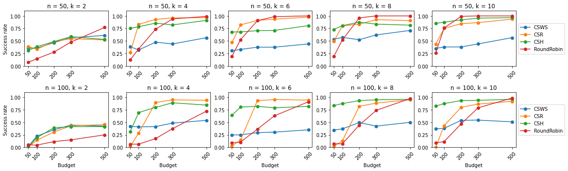
Refer to caption
Figure 3: Success rates of our proposed algorithms for varying nn, kk and budget BB in the reward setting.

The success rates of our proposed algorithms for identifying i∗i^{*} given a budget BB are shown in Figure 3. It is visible, that in particular for the challenging scenario, where the budget BB and the subset size kk are small and the number of arms nn is large, both CSH and CSR perform well. Especially CSH has overall a solid performance.

Reward setting.

In contrast to the experiments with reward feedback shown in the main paper, we try in the following experiments to force the generalized Borda winner to be different from the generalized Condorcet winner. For this purpose, we fix one random arm iℬ∗∈[n]\{i∗}i_{\mathcal{B}}^{\ast}\in[n]\backslash\{i^{\ast}\} as the prospective generalized Borda winner and set its expected value to μiℬ∗|Q=maxj∈Q,j≠iℬ∗⁡μj|Q+2​ϵ\mu_{i_{\mathcal{B}}^{\ast}|Q}=\max_{j\in Q,j\neq i_{\mathcal{B}}^{\ast}}\mu_{j|Q}+2\epsilon for any Q∈𝒬≤kQ\in\mathcal{Q}_{\leq k} with iℬ∗∈Qi_{\mathcal{B}}^{\ast}\in Q and i∗∉Qi^{\ast}\notin Q. Thus, iℬ∗i_{\mathcal{B}}^{\ast} is likely the generalized Borda winner and is different from the generalized Condorcet winner. Since our goal is to find the generalized Condorcet winner i∗i^{\ast}, RoundRobin will probably fail most of the times in finding i∗.i^{\ast}. This is due to the fact that RoundRobin focuses on identifying iℬ∗,i_{\mathcal{B}}^{\ast}, i.e., the the generalized Borda winner, which, however, does not coincidence with the generalized Condorcet winner i∗i^{\ast}.

This suspicion is confirmed by the results of the experiments shown in Figure 4 illustrating the empirical success rates for finding the generalized Condorcet winner in the setting described above. Except for some cases where the subset size kk is relatively large in comparison to the total number of arms, such that the generalized Condorcet winner is already contained in most of the seen subsets and hence is automatically also the generalized Borda winner, RoundRobin performs poorly in finding the generalized Condorcet winner and is always outperformed by the algorithms based on the combinatorial successive elimination strategy in Section 4.1.

Refer to caption
Figure 4: Success rates of our proposed algorithms for varying nn, kk and budget BB in the reward setting with different generalized Condorcet winner and generalized Borda winner.

Preference-based setting with different GCW and GBW.

In the preference-based setting we ignore the explicit numerical values of the observation vector and only use the information which arm was (not) the winner, i.e., which had (not) the highest observation value in the query set used , formally sij|Q(t)=1t∑s=1t𝟙{oij|Q(s)=maxi=i1,…​i|Q|oi|Q(s)}.s_{i_{j}|Q}(t)=\frac{1}{t}\sum_{s=1}^{t}\mathds{1}\{o_{i_{j}|Q}(s)=\max_{i=i_{1},\dots i_{|Q|}}o_{i|Q}(s)\}. Additionally, we fix one arm iℬ∗∈[n]\{i∗}i_{\mathcal{B}}^{\ast}\in[n]\backslash\{i^{\ast}\} and set μiℬ∗|Q=maxj∈Q,j≠iℬ∗⁡μj|Q+2​ε\mu_{i_{\mathcal{B}}^{\ast}|Q}=\max_{j\in Q,j\neq i_{\mathcal{B}}^{\ast}}\mu_{j|Q}+2\varepsilon for any QQ with iℬ∗∈Qi_{\mathcal{B}}^{\ast}\in Q and i∗∉Q.i^{\ast}\notin Q. In this way, iℬ∗i_{\mathcal{B}}^{\ast} is the generalized Borda winner and different from i∗.i^{\ast}.

The success rates of our proposed algorithms for identifying i∗i^{*} in this setting are shown in Figure 5. As expected our methods outperform RoundRobin in all scenarios.

Refer to caption
Figure 5: Success rates of our proposed algorithms for varying nn, kk and budget BB in the preference-based setting with different generalized Condorcet winner and generalized Borda winner.

Preference-based setting.

We now investigate the case, in which we do not force the generalized Borda winner and the generalized Condorcet winner to be different, thus they will naturally coincidence in most of the cases. This is achieved by considering the problem configuration as in the reward setting specified in Section 6, and ignoring the explicit numerical values (as in the preference-setting above).

The resulting success rates for finding the generalized Condorcet winner illustrated in Figure 6 are similar to the results in the reward setting for matching generalized Condorcet winner and generalized Borda winner. This means that, in particular, when the budget is small, the number of arms is large and the subset size is small, the algorithms following the combinatorial successive elimination strategy outperform RoundRobin. Note that this setting is arguably the most relevant setup for practical applications. Moreover, Figure 6 illustrates the natural effect one would expect for the number of arms nn on success rates, namely that success rates decrease with a larger number of arms.

Refer to caption
Figure 6: Success rates of our proposed algorithms for varying nn, kk and budget BB in the preference-based setting with (mostly) matching generalized Condorcet winner and generalized Borda winner.

G.2 Statistics beyond the Arithmetic Mean

We consider in the following the reward setting, where each observation is random sampled from the following distribution

𝒐Q​(t)∼𝒩⁡((μ1|Q⋮μ|Q||Q),(σ1|Q⋮σ|Q||Q))\displaystyle\bm{o}_{Q}(t)\sim\mathcal{N}\left(\left(\begin{array}[]{c}\mu_{1|Q}\\ \vdots\\ \mu_{|Q||Q}\end{array}\right),\left(\begin{array}[]{c}\sigma_{1|Q}\\ \vdots\\ \sigma_{|Q||Q}\end{array}\right)\right)

for μi|Q\mu_{i|Q} is sampled randomly from [0,1][0,1] and σi|Q\sigma_{i|Q} from [0.05,0.2][0.05,0.2] for each arm i∈Qi\in Q.

Median

An alternative to the arithmetic mean would be to measure the quality of the arms by the median of the seen observations. In particular, when the observations are prone to outliers, the median provides a more robust statistic: si|Q​(t)=Median​(oi|Q​(1),…,oi|Q​(t))s_{i|Q}(t)=\textsc{Median}(o_{i|Q}(1),\dots,o_{i|Q}(t)) for each arm i∈Qi\in Q. The results for this setting are illustrated in Figure 7.

Refer to caption
Figure 7: Success rates of our proposed algorithms for varying nn, kk and budget BB in the rewards setting with (mostly) matching generalized Condorcet winner and generalized Borda winner and using the median as the statistic.

Power-Mean

Another possibility is to use the so called power-mean, which is a compromise between the maximum and the arithmetic mean for a (multi)set of observations. Since the arithmetic mean is known to underestimate the true quality of an arm, while the maximum overestimates it, the power mean is often a good compromise, as it lies between the two. It is defined by si|Q​(t)=(1t​∑t′=1toi|Q​(t′)q)1/qs_{i|Q}(t)=\left(\frac{1}{t}\sum_{t^{\prime}=1}^{t}o_{i|Q}(t^{\prime})^{q}\right)^{1/q} for each arm i∈Qi\in Q and a fixed q∈ℕq\in\mathbb{N}. We use in the following q=2q=2. The results for this setting are illustrated in Figure 8.

Refer to caption
Figure 8: Success rates of our proposed algorithms for varying nn, kk and budget BB in the rewards setting with (mostly) matching generalized Condorcet winner and generalized Borda winner and using the power mean as the statistic.