MaskGIT: Masked Generative Image Transformer
Abstract
Generative transformers have experienced rapid popularity growth in the computer vision community in synthesizing high-fidelity and high-resolution images. The best generative transformer models so far, however, still treat an image naively as a sequence of tokens, and decode an image sequentially following the raster scan ordering (i.e. line-by-line). We find this strategy neither optimal nor efficient. This paper proposes a novel image synthesis paradigm using a bidirectional transformer decoder, which we term MaskGIT. During training, MaskGIT learns to predict randomly masked tokens by attending to tokens in all directions. At inference time, the model begins with generating all tokens of an image simultaneously, and then refines the image iteratively conditioned on the previous generation. Our experiments demonstrate that MaskGIT significantly outperforms the state-of-the-art transformer model on the ImageNet dataset, and accelerates autoregressive decoding by up to 64x. Besides, we illustrate that MaskGIT can be easily extended to various image editing tasks, such as inpainting, extrapolation, and image manipulation.
![[Uncaptioned image]](2202.04200v1/teaser1.png)
1 Introduction
Deep image synthesis as a field has seen a lot of progress in recent years. Currently holding state-of-the-art results are Generative Adversarial Networks (GANs), which are capable of synthesizing high-fidelity images at blazing speeds. They suffer from, however, well known issues include training instability and mode collapse, which lead to a lack of sample diversity. Addressing these issues still remains open research problems.
Inspired by the success of Transformer Vaswani17attention and GPT gpt3 in NLP, generative transformer models have received growing interests in image synthesis chen2020imagegpt; Esser21vqgan; Razavi19vqvae2. Generally, these approaches aim at modeling an image like a sequence and leveraging the existing autoregressive models to generate image. Images are generated in two stages; the first stage is to quantize an image to a sequence of discrete tokens (or visual words). In the second stage, an autoregressive model (e.g., transformer) is learned to generate image tokens sequentially based on the previously generated result (i.e. autoregressive decoding). Unlike the subtle min-max optimization used in GANs, these models are learned by maximum likelihood estimation. Because of the design differences, existing works have demonstrated their advantages over GANs in offering stabilized training and improved distribution coverage or diversity.
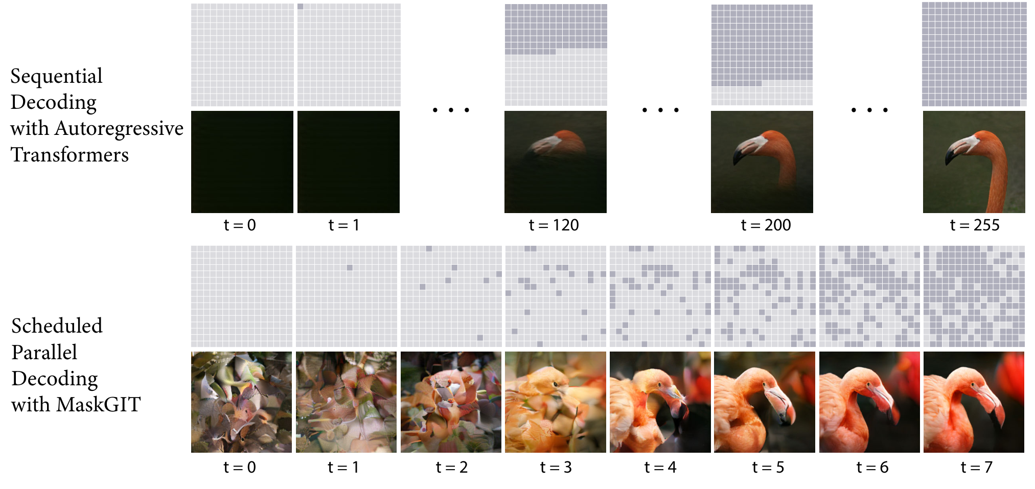
Existing works on generative transformers mostly focus on the first stage, i.e. how to quantize images such that information loss is minimized, and share the same second stage borrowed from NLP. Consequently, even the state-of-the-art generative transformers Esser21vqgan; Ramesh21dalle still treat an image naively as a sequence, where an image is flattened into a 1D sequence of tokens following a raster scan ordering, i.e. from left to right line-by-line (cf. Figure 2). We find this representation neither optimal nor efficient for images. Unlike text, images are not sequential. Imagine how an artwork is created. A painter starts with a sketch and then progressively refines it by filling or tweaking the details, which is in clear contrast to the line-by-line printing used in previous work chen2020imagegpt; Esser21vqgan. Additionally, treating image as a flat sequence means that the autoregressive sequence length grows quadratically, easily forming an extremely long sequence–longer than any natural language sentence. This poses challenges for not only modeling long-term correlation but also renders the decoding intractable. For example, it takes a considerable 30 seconds to generate a single image on a GPU autoregressively with 32x32 tokens.
This paper introduces a new bidirectional transformer for image synthesis called Masked Generative Image Transformer (MaskGIT). During training, MaskGIT is trained on a similar proxy task to the mask prediction in BERT Devlin19bert. At inference time, MaskGIT adopts a novel non-autoregressive decoding method to synthesize an image in constant number of steps. Specifically, at each iteration, the model predicts all tokens simultaneously in parallel but only keeps the most confident ones. The remaining tokens are masked out and will be re-predicted in the next iteration. The mask ratio is decreased until all tokens are generated with a few iterations of refinement. As illustrated in Figure 2, MaskGIT’s decoding is an order-of-magnitude faster than the autoregresive decoding as it only takes 8 steps, instead of 256 steps, to generate an image and the predictions within each step are parallelizable. Moreover, instead of conditioning only on previous tokens in the order of raster scan, bidirectional self-attention allows the model to generate new tokens from generated tokens in all directions. We find that the mask scheduling (i.e. fraction of the image masked each iteration) significantly affects generation quality. We propose to use the cosine schedule and substantiate its efficacy in the ablation study.
On the ImageNet benchmark, we empirically demonstrate that MaskGIT is both significantly faster (by up to 64x) and capable of generating higher quality samples than the state-of-the-art autoregressive transformer, i.e. VQGAN, on class-conditional generation with 256256 and 512512 resolution. Even compared with the leading GAN model, i.e. BigGAN, and diffusion model, i.e. ADM dhariwal2021diffusion, MaskGIT offers comparable sample quality while yielding more favourable diversity. Notably, our model establishes new state-of-the-arts on classification accuracy score (CAS) Ravuri19CAS and on FIDFID for synthesizing 512512 images. To our knowledge, this paper provides the first evidence demonstrating the efficacy of the masked modeling for image generation on the common ImageNet benchmark.
Furthermore, MaskGIT’s multidirectional nature makes it readily extendable to image manipulation tasks that are otherwise difficult for autoregressive models. Fig. 1 shows a new application of class-conditional image editing in which MaskGIT re-generates content inside the bounding box based on the given class while keeping the context (outside of the box) unchanged. This task, which is either infeasible for autoregressive model or difficult for GAN models, is trivial for our model. Quantitatively, we demonstrate this flexibility by applying MaskGIT to image inpainting, and image extrapolation in arbitrary directions. Even though our model is not designed for such tasks, it obtains comparable performance to the dedicated models on each task.
2 Related Work
2.1 Image Synthesis
Deep generative models KingmaW14; Vahdat2020nvae; goodfellow2014generative; SAGAN; Song19generative; dhariwal2021diffusion; Oord16pixelcnn; Parmar18imagetransformer have achieved lots of successes in image synthesis tasks. GAN based methods demonstrate amazing capability in yielding high-fidelity samples goodfellow2014generative; biggan; Karras2019stylegan2; SAGAN; tseng2021regularizing. In contrast, likelihood-based methods, such as Variational Autoencoders (VAEs) KingmaW14; Vahdat2020nvae, Diffusion Models Song19generative; dhariwal2021diffusion; ho2021cascaded and Autoregressive Models Oord16pixelcnn; Parmar18imagetransformer, offer distribution coverage and hence can generate more diverse samples Song19generative; Vahdat2020nvae; Oord16pixelcnn.
However, maximizing likelihood directly in pixel space can be challenging. So instead, VQVAE Oord17vqvae; Razavi19vqvae2 proposes to generate images in latent space in two stages. In the first stage, which is known as tokenization, it tries to compress images into discrete latent space, and primarily consists of three components:
- •
an encoder that learns to tokenize images into latent embedding ,
- •
a codebook which serves for a nearest neighbor look up used to quantize the embedding into visual tokens, and
- •
a decoder which predicts the reconstructed image from the visual tokens .
In the second stage, it first predicts the latent priors of the visual tokens using deep autoregressive models, and then uses the decoder from the first stage to map the token sequences into image pixels. Several approaches have followed this paradigm due to the efficacy of the two-stage approach. DALL-E Ramesh21dalle uses Transformers Vaswani17attention to improve token prediction in the second stage. VQGAN Esser21vqgan adds adversarial loss and perceptual loss johnson2016perceptual; zhang2018unreasonable in the first stage to improve the image fidelity. A contemporary work to ours, VIM vim2021, proposes to use a VIT backbone dosovitskiy2021vit to further improve the tokenization stage. Since these approaches still employ an auto-regressive model, the decoding time in the second stage scales with the token sequence length.
2.2 Masked Modeling with Bi-directional Transformers
The transformer architecture Vaswani17attention, was first proposed in NLP, and has recently extended its reach to computer vision dosovitskiy2021vit; caron2021dino. Transformer consists of multiple self-attention layers, allowing interactions between all pairs of elements in the sequence to be captured. In particular, BERT Devlin19bert introduces the masked language modeling (MLM) task for language representation learning. The bi-directional self-attention used in BERT Devlin19bert allows the masked tokens in MLM to be predicted utilizing context from both directions. In vision, the masked modeling in BERT Devlin19bert has been extended to image representation learning he2021mae; Bao2022Beit with images quantized to discrete tokens. However, few works have successfully applied the same masked modeling to image generation zhang2021ufcbert because of the difficulty in performing autoregressive decoding using bi-directional attentions. To our knowledge, this paper provides the first evidence demonstrating the efficacy of masked modeling for image generation on the common ImageNet benchmark. Our work is inspired by bi-directional machine translation ghazvininejad2019maskpredict; gu2020fully; gu2017non in NLP, and our novelty lies in the proposed new masking strategy and decoding algorithm which, as substantiated by our experiments, are essential for image generation.

3 Method
Our goal is to design a new image synthesis paradigm utilizing parallel decoding and bi-directional generation.
We follow the two-stage recipe discussed in 2.1, as illustrated in Figure 3. Since our goal is to improve the second stage, we employ the same setup for the first stage as in the VQGAN model Esser21vqgan, and leave potential improvements to the tokenization step to future work.
For the second stage, we propose to learn a bidirectional transformer by Masked Visual Token Modeling (MVTM). We introduce MVTM training in 3.1 and the sampling procedure in 3.2. We then discuss the key technique of masking design in 3.3.
3.1 MVTM in Training
Let denote the latent tokens obtained by inputting the image to the VQ-encoder, where is the length of the reshaped token matrix, and the corresponding binary mask. During training, we sample a subset of tokens and replace them with a special [MASK] token. The token is replaced with [MASK] if , otherwise, when , will be left intact.
The sampling procedure is parameterized by a mask scheduling function , and executes as follows: we first sample a ratio from to , then uniformly select tokens in to place masks, where is the length. The mask scheduling significantly affects the quality of image generation and will be discussed in 3.3.
Denote the result after applying mask to . The training objective is to minimize the negative log-likelihood of the masked tokens:
| (1) |
Concretely, we feed the masked into a multi-layer bidirectional transformer to predict the probabilities for each masked token, where the negative log-likelihood is computed as the cross-entropy between the ground-truth one-hot token and predicted token. Notice the key difference to autoregressive modeling: the conditional dependency in MVTM has two directions, which allows image generation to utilize richer contexts by attending to all tokens in the image.
3.2 Iterative Decoding
In autoregressive decoding, tokens are generated sequentially based on previously generated output. This process is not parallelizable and thus very slow for image because the image token length, e.g. 256 or 1024, is typically much larger than that of language. We introduce a novel decoding method where all tokens in the image are generated simultaneously in parallel. This is feasible due to the bi-directional self-attention of MTVM.
In theory, our model is able to infer all tokens and generate the entire image in a single pass. We find this challenging due to inconsistency with the training task. Below, the proposed iterative decoding is introduced. To generate an image at inference time, we start from a blank canvas with all the tokens masked out, i.e. . For iteration , our algorithm runs as follows:
- 1.
Predict. Given the masked tokens at the current iteration, our model predicts the probabilities, denoted as , for all the masked locations in parallel.
- 2.
Sample. At each masked location , we sample a token based on its prediction probabilities over all possible tokens in the codebook. After a token is sampled, its corresponding prediction score is used as a “confidence” score indicating the model’s belief of this prediction. For the unmasked position in , we simply set its confidence score to .
- 3.
Mask Schedule. We compute the number of tokens to mask according to the mask scheduling function by , where is the input length and is the total number of iterations.
- 4.
Mask. We obtain by masking tokens in . The mask for iteration is calculated from:
where is the confidence score for the -th token.
The decoding algorithm synthesizes an image in steps. At each iteration, the model predicts all tokens simultaneously but only keeps the most confident ones. The remaining tokens are masked out and re-predicted in the next iteration. The mask ratio is made decreasing until all tokens are generated within iterations. In practice, the masking tokens are randomly sampled with temperature annealing to encourage more diversity, and we will discuss its effect in 3. Figure 2 illustrates an example of our decoding process. It generates an image in iterations, where the unmasked tokens at each iteration are highlighted in the grid, e.g. when we only keep 1 token and mask out the rest.
3.3 Masking Design
We find that the quality of image generation is significantly affected by the masking design. We model the masking procedure by a mask scheduling function that computes the mask ratio for the given latent tokens. As discussed, the function is used in both training and inference. During inference time, it takes the input of indicating the progress in decoding. In training, we randomly sample a ratio in to simulate the various decoding scenarios.
BERT uses a fixed mask ratio of 15% Devlin19bert, i.e., it always masks 15% of the tokens, which is unsuitable for our task since our decoder needs to generate images from scratch. New masking scheduling is thus needed. Before discussing specific schemes, we first examine the property of the mask scheduling function. First, needs to be a continuous function bounded between and for . Second, should be (monotonically) decreasing with respect to , and it holds that and . The second property ensures the convergence of our decoding algorithm.
This paper considers common functions and makes simple transformations so that they satisfy the properties. Figure 8 visualizes these functions which are divided into three groups:
- •
Linear function is a straightforward solution, which masks an equal amount of tokens each time.
- •
Concave function captures the intuition that image generation follows a less-to-more information flow. In the beginning, most tokens are masked so the model only needs to make a few correct predictions for which the model feel confident. Towards the end, the mask ratio sharply drops, forcing the model to make a lot more correct predictions. The effective information is increasing in this process. The concave family includes cosine, square, cubic, and exponential.
- •
Convex function, conversely, implements a more-to-less process. The model needs to finalize a vast majority of tokens within the first couple of iterations. This family includes square root and logarithmic.
We empirically compare the above mask scheduling functions in 3 and find the cosine function works the best in all of our experiments.
4 Experiments
In this section, we empirically evaluate MaskGIT on image generation in terms of quality, efficiency and flexibility. In 4.2, we evaluate MaskGIT on the standard class-conditional image generation tasks on ImageNet deng2009imagenet 256256 and 512512. In 4.3, we show MaskGIT’s versatility by demonstrating its performance on three image editing tasks, image inpainting, outpainting, and editing. In 3, we verify the necessity of our design of mask scheduling. We will release the code and model for reproducible research.
4.1 Experimental Setup
For each dataset, we only train a single autoencoder, decoder, and codebook with 1024 tokens on cropped 256x256 images for all the experiments. The image is always compressed by a fixed factor of 16, i.e. from to a grid of tokens in the size of , where = and =. We find that this autoencoder, together with the codebook, can be reused to synthesize 512512 images.
All models in this work have the same configuration: 24 layers, 8 attention heads, 768 embedding dimensions and 3072 hidden dimensions. Our models use learnable positional embeddingVaswani17attention, LayerNormba2016layer, and truncated normal initialization (stddev=). We employ the following training hyperparameters: label smoothing=, dropout rate=, Adam optimizer kingma2014adam with = and =. We use RandomResizeAndCrop for data augmentation. All models are trained on 4x4 TPU devices with a batch size of 256. ImageNet models are trained for 300 epochs while the Places2 model is trained for 200 epochs.
4.2 Class-conditional Image Synthesis
We evaluate the performance of our model on class-conditional image synthesis on ImageNet 256256 and 512512. Our main results are summarized in Table 1.
Quality. On ImageNet 256256, without any special sampling strategies such as beam-search, top-k or nucleus sampling heuristics holtzman2019nucleus or classifier guidance Razavi19vqvae2, we significantly outperform VQGAN Esser21vqgan in both Fréchet Inception Distance (FID) FID ( vs ) and Inception Score (IS) ( vs ). We also report the results with classifier-based rejection sampling in the appendix B.
We also train a VQGAN baseline with the same tokenizer and hyperparameters as MaskGIT’s in order to further highlight the difference between bi-directional and uni-directional transformers, and find that on both resolutions, MaskGIT still outperforms our implemented baseline by a significant margin.
Furthermore, MaskGIT improves BigGAN’s FIDs on both resolutions, achieving a new state-of-the-art on 512512 with an FID of .
| Model | FID | IS | Prec | Rec | # params | # steps | CAS | |||||
| Top-1 (76.6) | Top-5 (93.1) | |||||||||||
| ImageNet 256256 | ||||||||||||
| DCTransformer nash2021generating □ | 36.51 | n/a | 0.36 | 0.67 | 738M | 1024 | ||||||
| BigGAN-deep biggan | 6.95 | 198.2 | 0.87 | 0.28 | 160M | 1 | 43.99 | 67.89 | ||||
| Improved DDPM nichol2021improved□ | 12.26 | n/a | 0.70 | 0.62 | 280M | 250 | ||||||
| ADM dhariwal2021diffusion□ | 10.94 | 101.0 | 0.69 | 0.63 | 554M | 250 | ||||||
| VQVAE-2 Razavi19vqvae2□ | 31.11 | 45 | 0.36 | 0.57 | 13.5B† | 5120 | 54.83 | 77.59 | ||||
| VQGAN Esser21vqgan□ | 15.78 | 78.3 | n/a | n/a | 1.4B | 256 | ||||||
| VQGAN∗ | 18.65 | 80.4 | 0.78 | 0.26 | 227M | 256 | 53.10 | 76.18 | ||||
| MaskGIT (Ours) | 6.18 | 182.1 | 0.80 | 0.51 | 227M | 8 | 63.14 | 84.45 | ||||
| ImageNet 512512 | ||||||||||||
| BigGAN-deep biggan | 8.43 | 232.5 | 0.88 | 0.29 | 160M | 1 | 44.02 | 68.22 | ||||
| ADM dhariwal2021diffusion□ | 23.24 | 58.06 | 0.73 | 0.60 | 559M | 250 | ||||||
| VQGAN∗ | 26.52 | 66.8 | 0.73 | 0.31 | 227M | 1024 | 51.29 | 74.24 | ||||
| MaskGIT (Ours) | 7.32 | 156.0 | 0.78 | 0.50 | 227M | 12 | 63.43 | 84.79 | ||||
 |
 |
 |
 |
 |
 |
 |
 |
 |
| BigGAN-deep (FID=) | MaskGIT (FID=6.18) | Training Set |
 |
 |
 |
 |
 |
 |
 |
 |
 |
 |
 |
 |
 |
 |
 |
 |
 |
 |
 |
 |
 |
 |
 |
 |
| Input | —— MaskGIT (Our Samples) —— | ||
| Task | Model | FID | IS | ||
|---|---|---|---|---|---|
| Outpainting | Boundless teterwak2019boundless□ | 35.02 | 6.15 | ||
| Right 50% | In&Out cheng2021inout□ | 23.57 | 7.18 | ||
| InfinityGAN lin2021infinitygan | 10.60 | 5.57 | |||
| Boundless teterwak2019boundless TF ◆ | 7.80 | 5.99 | |||
| MaskGIT (Ours) 512 | 6.78 | 11.69 | |||
| Inpainting | DeepFill yu2019free | 11.51 | 22.55 | ||
| Center 50%50% | ICTwan2021ict† | 13.63 | 17.70 | ||
| HiFill yi2020contextual512 | 16.60 | 19.93 | |||
| CoModGANzhao2021comodgan512 | 7.13 | 21.82 | |||
| MaskGIT (Ours)512 | 7.92 | 22.95 |
Speed. We evaluate model speed by assessing the number of steps, i.e. forward passes, each model requires to generate a sample. As shown in Table 1, MaskGIT requires the fewest steps among all non-GAN-based models on both resolutions.
To further substantiate the speed difference between MaskGIT and autoregressive models, we perform a runtime comparison between MaskGIT and VQGAN’s decoding processes. As illustrated in Figure 4, MaskGIT significantly accelerates VQGAN by -x, with a speedup that gets more pronounced as the image resolution (and thus the input token length) grows.
Diversity. We consider Classification Accuracy Score (CAS) Ravuri19CAS and Precision/Recall KynkaanniemiKLL19 as two metrics for evaluating sample diversity, in addition to sample quality.
CAS involves first training a ResNet-50 classifierResNet solely on the samples generated by the candidate model, and then measuring the classifier’s classification accuracy on the ImageNet validation set. The last two columns in Table 1 present the CAS results, where the scores of the classifier trained on real ImageNet training data are included for reference (76.6% and 93.1% for the top-1 and top-5 accuracy). For image resolution 256256, we follow the common practice of using data augmentation RandAugmentcubuk2019randaugment, and report the scores trained without augmentation in the appendix B. We find that MaskGIT significantly outperforms prior work VQVAE-2 and VQGAN, establishing a new state-of-the-art of CAS on the ImageNet benchmark on both resolutions.
The Precision/Recall results in Table 1 show that MaskGIT achieves better coverage (Recall) compared to BigGAN, and better sample quality (Precision) compared to likelihood-based models such as VQVAE-2 and diffusion models. Compared to our baseline VQGAN, we improve the diversity as measured by recall while slightly boosting its precision.
4.3 Image Editing Applications
In this subsection, we present direct applications of MaskGIT on three image editing tasks: class-conditional image editing, image inpainting, and outpainting. All three tasks can be almost trivially translated to ones that MaskGIT can handle if we consider the task as just a constraint on the initial binary mask MaskGIT uses in its iterative decoding, as discussed in 3.2. We show that without modifications to the architecture or any task-specific training, MaskGIT is capable of generating very compelling results on all three applications. Furthermore, MaskGIT obtains comparable performance to dedicated models on both inpainting and outpainiting, even though it is not designed specifically for either task.
Class-conditional Image Editing. We define a new class-conditional image editing task to showcase MaskGIT’s flexibility. In this task, the model regenerates content specified inside a bounding box on the given class while preserving the context, i.e. content outside of the box. It is infeasible for autoregressive methods due to the violation to their prediction orders.
For MaskGIT, however, it is a trivial task if we consider the bounding box region as the input of initial mask to the iterative decoding algorithm. Figure 6 shows a few example results. More can be found in the appendix C.
In these examples, we observe that MaskGIT can reasonably replace the selected object while preserving, or to some extend even completing, the context in the background. Furthermore, we find that MaskGIT seems to be capable of synthesizing unnatural yet plausible combinations unseen in the ImageNet training set, e.g. a flying cat, cat in a soup bowl, and cat in a flower. This suggests that MaskGIT has incidentally learned useful representations for composition, which may be further exploited in related tasks in future works.
Image Inpainting. Image inpainting or image completion is a fundamental image editing task to synthesize contents in missing regions so that the completion looks visually realistic. Traditional patch-based methodsBarnes:2009:patchmatch work well on texture regions, while deep learning based methodsyu2019free; yi2020contextual; zhao2021comodgan; saharia2021palette; esser2021imagebart have been demonstrated to synthesize images requiring better semantic coherence. Both approaches have been are extensively studied in computer vision.
We extend MaskGIT to this problem by tokenizing the masked image and interpreting the inpainting mask as the initial mask in our iterative decoding. We then composite the output image by linearly blending it with the input based on the masking boundary following cheng2021inout. To match the training of our baselines, we train MaskGIT on the 512512 center-cropped images from the Places2zhou2017places dataset. All hyperparameters are kept the same as the MaskGIT model trained on ImageNet.
We compare MaskGIT against common GAN-based baselines, including DeepFillv2yu2019free and HiFillyi2020contextual, on inpainting with a central 50% 50% mask, which are evaluated on the Places2 validation set. Table 2 summarizes the quantitative comparisons. MaskGIT beats both DeepFill and HiFill in FID and IS by a significant margin, while achieving scores close to the state-of-the-art inpainting approach CoModGAN zhao2021comodgan. We show more qualitative comparisons with CoModGAN in the appendix E.
Image Outpainting. Outpainting, or image extrapolation, is an image editing task that has received increased attention recently. It is seen as a more challenging task than inpainting due to the fewer constraints from surrounding pixels and thus more uncertainty in the predicted regions. Our adaptation of the problem and the model used in the following evaluation is the same as in inpainting.
We compare against common GAN-based baselines, including Boundless teterwak2019boundless, In&Out cheng2021inout, InfinityGANlin2021infinitygan, and CoModGANzhao2021comodgan on extrapolating rightward with a 50% ratio. We evaluate on the image set generously provided by the authors of InfinityGANlin2021infinitygan and In&Outcheng2021inout.
Table 2 summarizes the quantitative comparisons. MaskGIT beats all baselines and achieves state-of-the-art FID and IS. As the examples in Figure 7 illustrate, MaskGIT is also capable of synthesizing diverse results given the same input with different seeds. We observe that MaskGIT completes objects and global structures particularly well, and hypothesize that this is thanks to the model learning useful representations with the global attentions in the transformer.
4.4 Ablation Studies
| FID | IS | NLL | |||
|---|---|---|---|---|---|
| Exponential | 8 | 7.89 | 156.3 | 4.83 | |
| Cubic | 9 | 7.26 | 165.2 | 4.63 | |
| Square | 10 | 6.35 | 179.9 | 4.38 | |
| Cosine | 10 | 6.06 | 181.5 | 4.22 | |
| Linear | 16 | 7.51 | 113.2 | 3.75 | |
| Square Root | 32 | 12.33 | 99.0 | 3.34 | |
| Logarithmic | 60 | 29.17 | 47.9 | 3.08 |
We conduct ablation experiments using the default setting on ImageNet 256256.
Mask scheduling. A key design of MaskGIT is the mask scheduling function used in both training and iterative decoding. We compare the functions discussed in 3.3, visualize them in Figure 8, and summarize the results in Table 3.
We observe that concave functions generally obtain better FID and IS than linear, followed by the convex functions. While cosine and square perform similarly relative to other functions, cosine slightly edges out square in all scores, making cosine the default in our model.
We hypothesize that concave functions perform favorably because they 1) challenge training with more difficult cases (i.e. encouraging larger mask ratios), and 2) appropriately prioritize the less-to-more prediction throughout the decoding. That said, over-prioritization seems to be costly as well, as shown by the cubic function being worse than square, and exponential being much worse than all other concave functions.
Iteration number. We study the effect of the number of iterations () on our model by running all candidate masking functions with different s. As shown in Figure 8, under the same setting, more iterations are not necessarily better: as increases, aside from the logarithmic function which performs poorly throughout, all other functions hit a “sweet spot” where the model’s performance peaks before it worsens again. The sweet spot also gets “delayed” as functions get less concave. As shown, among functions that achieve strong FIDs (i.e. cosine, square, and linear), cosine not only has the strongest overall score, but also the earliest sweet spot at a total of to iterations. We hypothesize that such sweet spots exist because too many iterations may discourage the model from keeping less confident predictions, which worsens the token diversity. We think further study on the masking design would be interesting for future work.
5 Conclusion
In this paper, we propose MaskGIT, a novel image synthesis paradigm using a bidirectional transformer decoder. Trained on Masked Visual Token Modeling, MaskGIT learns to generate samples using an iterative decoding process within a constant number of iterations. Experimental results show that MaskGIT significantly outperforms the state-of-the-art transformer model on conditional image generation, and our model is readily extendable to various image manipulation tasks. As MaskGIT achieves competitive performance with state-of-the-art GANs, applying our approach to other synthesis tasks is a promising direction for future work. Please see the appendix F for the limitations and future work.
Acknowledgement The authors would like to thank Xiang Kong for inspiring related works and anonymous reviewers for helpful comments.
References
- (1) Jimmy Lei Ba, Jamie Ryan Kiros, and Geoffrey E. Hinton. Layer normalization, 2016.
- (2) Hangbo Bao, Li Dong, Songhao Piao, and Furu Wei. BEit: BERT pre-training of image transformers. In International Conference on Learning Representations, 2022.
- (3) Connelly Barnes, Eli Shechtman, Adam Finkelstein, and Dan B Goldman. PatchMatch: A randomized correspondence algorithm for structural image editing. ACM Transactions on Graphics (Proc. SIGGRAPH), 28(3), Aug. 2009.
- (4) Andrew Brock, Jeff Donahue, and Karen Simonyan. Large scale gan training for high fidelity natural image synthesis. In ICLR, 2019.
- (5) Tom Brown, Benjamin Mann, Nick Ryder, Melanie Subbiah, Jared D Kaplan, Prafulla Dhariwal, Arvind Neelakantan, Pranav Shyam, Girish Sastry, Amanda Askell, Sandhini Agarwal, Ariel Herbert-Voss, Gretchen Krueger, Tom Henighan, Rewon Child, Aditya Ramesh, Daniel Ziegler, Jeffrey Wu, Clemens Winter, Chris Hesse, Mark Chen, Eric Sigler, Mateusz Litwin, Scott Gray, Benjamin Chess, Jack Clark, Christopher Berner, Sam McCandlish, Alec Radford, Ilya Sutskever, and Dario Amodei. Language models are few-shot learners. In NeurIPS, 2020.
- (6) Mathilde Caron, Hugo Touvron, Ishan Misra, Hervé Jégou, Julien Mairal, Piotr Bojanowski, and Armand Joulin. Emerging properties in self-supervised vision transformers. In Proceedings of the International Conference on Computer Vision (ICCV), 2021.
- (7) Mark Chen, Alec Radford, Rewon Child, Jeffrey Wu, Heewoo Jun, David Luan, and Ilya Sutskever. Generative pretraining from pixels. In International Conference on Machine Learning, pages 1691–1703. PMLR, 2020.
- (8) Yen-Chi Cheng, Chieh Hubert Lin, Hsin-Ying Lee, Jian Ren, Sergey Tulyakov, and Ming-Hsuan Yang. In&out: Diverse image outpainting via gan inversion. arXiv preprint arXiv:2104.00675, 2021.
- (9) Ekin D. Cubuk, Barret Zoph, Jonathon Shlens, and Quoc V. Le. Randaugment: Practical automated data augmentation with a reduced search space, 2019.
- (10) Jia Deng, Wei Dong, Richard Socher, Li-Jia Li, Kai Li, and Li Fei-Fei. Imagenet: A large-scale hierarchical image database. In 2009 IEEE conference on computer vision and pattern recognition, pages 248–255. Ieee, 2009.
- (11) Jacob Devlin, Ming-Wei Chang, Kenton Lee, and Kristina Toutanova. BERT: pre-training of deep bidirectional transformers for language understanding. In Jill Burstein, Christy Doran, and Thamar Solorio, editors, NAACL-HLT, 2019.
- (12) Prafulla Dhariwal and Alexander Quinn Nichol. Diffusion models beat GANs on image synthesis. In A. Beygelzimer, Y. Dauphin, P. Liang, and J. Wortman Vaughan, editors, Advances in Neural Information Processing Systems, 2021.
- (13) Alexey Dosovitskiy, Lucas Beyer, Alexander Kolesnikov, Dirk Weissenborn, Xiaohua Zhai, Thomas Unterthiner, Mostafa Dehghani, Matthias Minderer, Georg Heigold, Sylvain Gelly, Jakob Uszkoreit, and Neil Houlsby. An image is worth 16x16 words: Transformers for image recognition at scale. In ICLR, 2021.
- (14) Patrick Esser, Robin Rombach, Andreas Blattmann, and Björn Ommer. Imagebart: Bidirectional context with multinomial diffusion for autoregressive image synthesis, 2021.
- (15) Patrick Esser, Robin Rombach, and Björn Ommer. Taming transformers for high-resolution image synthesis. In CVPR, 2021.
- (16) Marjan Ghazvininejad, Omer Levy, Yinhan Liu, and Luke Zettlemoyer. Mask-predict: Parallel decoding of conditional masked language models, 2019.
- (17) Ian Goodfellow, Jean Pouget-Abadie, Mehdi Mirza, Bing Xu, David Warde-Farley, Sherjil Ozair, Aaron Courville, and Yoshua Bengio. Generative adversarial nets. In NeurIPS, 2014.
- (18) Google. Tfhub model of boundless. https://tfhub.dev/google/boundless/half/1, 2021.
- (19) Jiatao Gu, James Bradbury, Caiming Xiong, Victor OK Li, and Richard Socher. Non-autoregressive neural machine translation. In ICLR, 2018.
- (20) Jiatao Gu and Xiang Kong. Fully non-autoregressive neural machine translation: Tricks of the trade, 2020.
- (21) Kaiming He, Xinlei Chen, Saining Xie, Yanghao Li, Piotr Dollár, and Ross Girshick. Masked autoencoders are scalable vision learners, 2021.
- (22) Kaiming He, Xiangyu Zhang, Shaoqing Ren, and Jian Sun. Deep residual learning for image recognition. In CVPR, 2016.
- (23) Martin Heusel, Hubert Ramsauer, Thomas Unterthiner, Bernhard Nessler, and Sepp Hochreiter. Gans trained by a two time-scale update rule converge to a local nash equilibrium. In NeurIPS, 2017.
- (24) Jonathan Ho, Chitwan Saharia, William Chan, David J Fleet, Mohammad Norouzi, and Tim Salimans. Cascaded diffusion models for high fidelity image generation. arXiv preprint arXiv:2106.15282, 2021.
- (25) Ari Holtzman, Jan Buys, Li Du, Maxwell Forbes, and Yejin Choi. The curious case of neural text degeneration, 2019.
- (26) Justin Johnson, Alexandre Alahi, and Li Fei-Fei. Perceptual losses for real-time style transfer and super-resolution. In European conference on computer vision, pages 694–711. Springer, 2016.
- (27) Tero Karras, Samuli Laine, Miika Aittala, Janne Hellsten, Jaakko Lehtinen, and Timo Aila. Analyzing and improving the image quality of StyleGAN. In CVPR, 2020.
- (28) Diederik P Kingma and Jimmy Ba. Adam: A method for stochastic optimization. arXiv preprint arXiv:1412.6980, 2014.
- (29) Diederik P. Kingma and Max Welling. Auto-encoding variational bayes. In ICLR, 2014.
- (30) Tuomas Kynkäänniemi, Tero Karras, Samuli Laine, Jaakko Lehtinen, and Timo Aila. Improved precision and recall metric for assessing generative models. In NeurIPS, 2019.
- (31) Chieh Hubert Lin, Hsin-Ying Lee, Yen-Chi Cheng, Sergey Tulyakov, and Ming-Hsuan Yang. Infinitygan: Towards infinite-resolution image synthesis. arXiv preprint arXiv:2104.03963, 2021.
- (32) Charlie Nash, Jacob Menick, Sander Dieleman, and Peter W. Battaglia. Generating images with sparse representations, 2021.
- (33) Alex Nichol and Prafulla Dhariwal. Improved denoising diffusion probabilistic models. arXiv preprint arXiv:2102.09672, 2021.
- (34) Niki Parmar, Ashish Vaswani, Jakob Uszkoreit, Lukasz Kaiser, Noam Shazeer, Alexander Ku, and Dustin Tran. Image transformer. In Jennifer G. Dy and Andreas Krause, editors, ICML, 2018.
- (35) Aditya Ramesh, Mikhail Pavlov, Gabriel Goh, Scott Gray, Chelsea Voss, Alec Radford, Mark Chen, and Ilya Sutskever. Zero-shot text-to-image generation. In Marina Meila and Tong Zhang, editors, ICML, 2021.
- (36) Suman V. Ravuri and Oriol Vinyals. Classification accuracy score for conditional generative models. In Hanna M. Wallach, Hugo Larochelle, Alina Beygelzimer, Florence d’Alché Buc, Emily B. Fox, and Roman Garnett, editors, NeurIPS, pages 12247–12258, 2019.
- (37) Ali Razavi, Aäron van den Oord, and Oriol Vinyals. Generating diverse high-fidelity images with VQ-VAE-2. In Hanna M. Wallach, Hugo Larochelle, Alina Beygelzimer, Florence d’Alché-Buc, Emily B. Fox, and Roman Garnett, editors, NeurIPS, 2019.
- (38) Chitwan Saharia, William Chan, Huiwen Chang, Chris A. Lee, Jonathan Ho, Tim Salimans, David J. Fleet, and Mohammad Norouzi. Palette: Image-to-image diffusion models, 2021.
- (39) Kim Seonghyeon. Implementation of generating diverse high-fidelity images with vq-vae-2 in pytorch. https://github.com/rosinality/vq-vae-2-pytorch, 2020.
- (40) Karen Simonyan and Andrew Zisserman. Very deep convolutional networks for large-scale image recognition, 2015.
- (41) Yang Song and Stefano Ermon. Generative modeling by estimating gradients of the data distribution. In Hanna M. Wallach, Hugo Larochelle, Alina Beygelzimer, Florence d’Alché-Buc, Emily B. Fox, and Roman Garnett, editors, NeurIPS, 2019.
- (42) Christian Szegedy, Vincent Vanhoucke, Sergey Ioffe, Jon Shlens, and Zbigniew Wojna. Rethinking the inception architecture for computer vision. In 2016 IEEE Conference on Computer Vision and Pattern Recognition (CVPR), pages 2818–2826, 2016.
- (43) Piotr Teterwak, Aaron Sarna, Dilip Krishnan, Aaron Maschinot, David Belanger, Ce Liu, and William T Freeman. Boundless: Generative adversarial networks for image extension. In Proceedings of the IEEE/CVF International Conference on Computer Vision, pages 10521–10530, 2019.
- (44) Hung-Yu Tseng, Lu Jiang, Ce Liu, Ming-Hsuan Yang, and Weilong Yang. Regularizing generative adversarial networks under limited data. In CVPR, 2021.
- (45) Arash Vahdat and Jan Kautz. NVAE: A deep hierarchical variational autoencoder. In Hugo Larochelle, Marc’Aurelio Ranzato, Raia Hadsell, Maria-Florina Balcan, and Hsuan-Tien Lin, editors, NeurIPS, 2020.
- (46) Aäron van den Oord, Nal Kalchbrenner, Lasse Espeholt, Koray Kavukcuoglu, Oriol Vinyals, and Alex Graves. Conditional image generation with pixelcnn decoders. In Daniel D. Lee, Masashi Sugiyama, Ulrike von Luxburg, Isabelle Guyon, and Roman Garnett, editors, NeurIPS, 2016.
- (47) Aäron van den Oord, Oriol Vinyals, and Koray Kavukcuoglu. Neural discrete representation learning. In Isabelle Guyon, Ulrike von Luxburg, Samy Bengio, Hanna M. Wallach, Rob Fergus, S. V. N. Vishwanathan, and Roman Garnett, editors, NeurIPS, 2017.
- (48) Ashish Vaswani, Noam Shazeer, Niki Parmar, Jakob Uszkoreit, Llion Jones, Aidan N. Gomez, Lukasz Kaiser, and Illia Polosukhin. Attention is all you need. In NeurIPS, 2017.
- (49) Ziyu Wan, Jingbo Zhang, Dongdong Chen, and Jing Liao. High-fidelity pluralistic image completion with transformers. arXiv preprint arXiv:2103.14031, 2021.
- (50) Zili Yi, Qiang Tang, Shekoofeh Azizi, Daesik Jang, and Zhan Xu. Contextual residual aggregation for ultra high-resolution image inpainting. In Proceedings of the IEEE/CVF Conference on Computer Vision and Pattern Recognition, pages 7508–7517, 2020.
- (51) Jiahui Yu, Xin Li, Jing Yu Koh, Han Zhang, Ruoming Pang, James Qin, Alexander Ku, Yuanzhong Xu, Jason Baldridge, and Yonghui Wu. Vector-quantized image modeling with improved VQGAN. arXiv preprint arXiv:2110.04627, 2021.
- (52) Jiahui Yu, Zhe Lin, Jimei Yang, Xiaohui Shen, Xin Lu, and Thomas S Huang. Free-form image inpainting with gated convolution. In Proceedings of the IEEE/CVF International Conference on Computer Vision, pages 4471–4480, 2019.
- (53) Han Zhang, Ian J. Goodfellow, Dimitris N. Metaxas, and Augustus Odena. Self-attention generative adversarial networks. In ICML, 2019.
- (54) Richard Zhang, Phillip Isola, Alexei A Efros, Eli Shechtman, and Oliver Wang. The unreasonable effectiveness of deep features as a perceptual metric. In Proceedings of the IEEE conference on computer vision and pattern recognition, pages 586–595, 2018.
- (55) Richard Zhang, Phillip Isola, Alexei A Efros, Eli Shechtman, and Oliver Wang. The unreasonable effectiveness of deep features as a perceptual metric. In CVPR, 2018.
- (56) Zhu Zhang, Jianxin Ma, Chang Zhou, Rui Men, Zhikang Li, Ming Ding, Jie Tang, Jingren Zhou, and Hongxia Yang. UFC-BERT: Unifying multi-modal controls for conditional image synthesis. In A. Beygelzimer, Y. Dauphin, P. Liang, and J. Wortman Vaughan, editors, Advances in Neural Information Processing Systems, 2021.
- (57) Shengyu Zhao, Jonathan Cui, Yilun Sheng, Yue Dong, Xiao Liang, Eric I Chang, and Yan Xu. Large scale image completion via co-modulated generative adversarial networks. In International Conference on Learning Representations (ICLR), 2021.
- (58) Bolei Zhou, Agata Lapedriza, Aditya Khosla, Aude Oliva, and Antonio Torralba. Places: A 10 million image database for scene recognition. IEEE Transactions on Pattern Analysis and Machine Intelligence, 2017.
| Original |
![[Uncaptioned image]](2202.04200v1/figures/analysis/cougar.jpeg)
|
![[Uncaptioned image]](2202.04200v1/figures/analysis/car.jpeg)
| ||||||||
| Mask 95% | Mask 90% | Mask 85% | Mask 75% | Mask 95% | Mask 90% | Mask 85% | Mask 75% | |||
| Example Input Mask |
![[Uncaptioned image]](2202.04200v1/figures/analysis/000286_39_mask03_95.jpeg)
|
![[Uncaptioned image]](2202.04200v1/figures/analysis/000286_0_mask01_90.jpeg)
|
![[Uncaptioned image]](2202.04200v1/figures/analysis/000286_2_mask_01_85.jpeg)
|
![[Uncaptioned image]](2202.04200v1/figures/analysis/000286_0_mask03_75.jpeg)
|
![[Uncaptioned image]](2202.04200v1/figures/analysis/000511_2_mask_95.jpeg)
|
![[Uncaptioned image]](2202.04200v1/figures/analysis/000511_0_mask_90.jpeg)
|
![[Uncaptioned image]](2202.04200v1/figures/analysis/000511_5_mask_85.jpeg)
|
![[Uncaptioned image]](2202.04200v1/figures/analysis/000511_0_mask_75.jpeg)
| ||
| Reconstruction Sample |
![[Uncaptioned image]](2202.04200v1/figures/analysis/000286_39_output_95.jpeg)
|
![[Uncaptioned image]](2202.04200v1/figures/analysis/000286_0_output_90.jpeg)
|
![[Uncaptioned image]](2202.04200v1/figures/analysis/cougar_85.jpeg)
|
![[Uncaptioned image]](2202.04200v1/figures/analysis/cougar_75.jpeg)
|
![[Uncaptioned image]](2202.04200v1/figures/analysis/car_95.jpeg)
|
![[Uncaptioned image]](2202.04200v1/figures/analysis/car_90.jpeg)
|
![[Uncaptioned image]](2202.04200v1/figures/analysis/car_85.jpeg)
|
![[Uncaptioned image]](2202.04200v1/figures/analysis/car_75.jpeg)
| ||
| Median of Samples |
![[Uncaptioned image]](2202.04200v1/figures/analysis/why_schedule_cougar_statistics_95percent_avg.jpeg)
|
![[Uncaptioned image]](2202.04200v1/figures/analysis/why_schedule_cougar_statistics_90percent_median.jpeg)
|
![[Uncaptioned image]](2202.04200v1/figures/analysis/why_schedule_cougar_85percent_median.jpeg)
|
![[Uncaptioned image]](2202.04200v1/figures/analysis/why_schedule_cougar_statistics_75percent_median.jpeg)
|
![[Uncaptioned image]](2202.04200v1/figures/analysis/why_schedule_car_statistics_95percent_median.jpeg)
|
![[Uncaptioned image]](2202.04200v1/figures/analysis/why_schedule_car_statistics_90percent_median.jpeg)
|
![[Uncaptioned image]](2202.04200v1/figures/analysis/why_schedule_car_statistics_85percent_median.jpeg)
|
![[Uncaptioned image]](2202.04200v1/figures/analysis/why_schedule_car_statistics1_75percent_median.jpeg)
|
Appendix A Discussion on Image Reconstruction
In 4.2, we primarily evaluate MaskGIT on class-conditional image generation tasks. Here we offer more discussion on its performance on image reconstruction. We set up by first randomly sampling input mask with a mask ratio of the visual tokens masked out, and then running MaskGIT’s iterative decoding algorithm to reconstruct images. Figure 10 shows the PSNR and LPIPSzhang2018lpips of the reconstructed samples as functions of , whereas Figure 9 visualizes two examples of this process with ranging from to .
We observe that MaskGIT reconstructs holistic information (e.g. pose and shape of the foreground objects) even with a very high percentage (e.g. 95%) of tokens masked out. More importantly, there seems to exist an inflection point around 90%: while both reconstruction quality and consistency improve drastically as the mask ratio decreases until 90%, after 90% further improvements are slowed down. This observation is corroborated by the large jump in the visual similarity between reconstruction samples and the original images from 95% to 90% in Figure 9, e.g. the fence in front of the tiger and the car’s color are consistently captured once the mask ratio is below 90%, but not at 95%.
In other words, we find that visual tokens are highly redundant. For a holistic reconstruction, only a very small portion (e.g. 10%) of the tokens are essential; the remaining ones merely improve the recovery of finer appearance or details. This echos our intuition behind the masking design laid out in 3.3 that the prediction of the first few tokens is key to image generation. Similar observations on the spatial redundancy of images are discussed in a concurrent paper MAE he2021mae. In their work, they find that masking a high proportion of the input image yields a nontrivial and meaningful self-supervisory task for image representation learning.
Appendix B Additional Class-conditional Image Generation Results
In this section, we report additional results on class-conditional image generation.
We follow prior transformer-based methodsRazavi19vqvae2; Esser21vqgan to employ the classifier-based rejection sampling to improve the sample quality scores. Specifically, we use a pre-trained ResNet classifierResNet to score output samples based on the predicted probability and keep samples with an acceptance rate of , as in VQGAN Esser21vqgan. As shown in Table 4, MaskGIT demonstrates consistent improvement over VQGAN, and is comparable with ADM with classifier guidance dhariwal2021diffusion. More importantly, by adding the rejection sampling, MaskGIT achieves state-of-the-art Inception Scores ( on 256256 and on 512512).
In Table 5, we report Precision and Recall scores calculated using Inception features christian16inception. In contrast to the VGGsimonyan2015vgg feature-based scores, which we report in Table 1 for a more direct comparison with prior work KynkaanniemiKLL19; dhariwal2021diffusion, we find that the Inception feature-based scores are more consistent with our qualitative observations that VQGAN’s samples are more diverse than BigGAN’s. Under both measures, MaskGIT ’s recall scores outperform those of BigGAN and VQGAN. We also report CAS evaluated on classifiers trained without augmentation from RandAugmentcubuk2019randaugment. Consistent with our main results, MaskGIT outperforms BigGAN and our baseline VQGAN by a large margin.
Finally, we show a few comparisons of the class-conditional samples generated by MaskGIT with the samples generated by BigGAN-deep and VQVAE-2 in Figure 11, 12, and 13.
| Dataset | Model | Classifier guidance | FID | IS | ||
|---|---|---|---|---|---|---|
| ImageNet | ADM dhariwal2021diffusion | 1.0 guidance | 4.59 | 186.70 | ||
| 256256 | VQGAN Esser21vqgan | 0.05 acceptance rate | 5.88 | 304.8 | ||
| MaskGIT | 0.05 acceptance rate | 4.02 | 355.6 | |||
| ImageNet | ADM dhariwal2021diffusion | 1.0 guidance | 7.72 | 172.71 | ||
| 512512 | MaskGIT | 0.05 acceptance rate | 4.46 | 342.0 |
| Model | Prec | Rec | CAS | |||
|---|---|---|---|---|---|---|
| Top-1 (73.1) | Top-5 (91.5) | |||||
| BigGAN-deep biggan | 0.82 | 0.27 | 42.65 | 65.92 | ||
| VQ-GAN∗ | 0.61 | 0.47 | 47.50 | 68.90 | ||
| MaskGIT (Ours) | 0.78 | 0.50 | 58.20 | 79.65 | ||
| BigGAN-deep (FID=) | VQVAE-2† (FID=) | MaskGIT (FID=6.18) |
|---|---|---|
 |
 |
 |
 |
 |
 |
| BigGAN-deep (FID=) | VQVAE-2 (FID=) | MaskGIT (FID=6.18) |
|---|---|---|
 |
 |
 |
 |
 |
 |
| BigGAN-deep (FID=) | VQVAE-2 (FID=) | MaskGIT (FID=6.18) |
|---|---|---|
 |
 |
 |
 |
 |
 |
Appendix C Additional Examples of Class-conditional Image Editing Applications
| Input Image |

|

|

|

|

| |
|---|---|---|---|---|---|---|
| Goldfish [001] |

|

|

|

|

| |
| Ice Bear [296] |

|

|

|

|

| |
| Argaric [992] |

|

|

|

|

| |
| Lorikeet [90] |

|

|

|

|

| |
| Train [829] |

|

|

|

|

| |
| Tiger [292] |

|

|

|

|

|
| Input | MaskGIT (Ours) |
|---|---|
 |
 |
 |
 |
 |
 |
 |
 |
 |
 |
 |
 |
Appendix D Image Outpainting Comparisons with SOTA Transformer-based Approaches
In Figure 16 and 17, we show a few outpainting comparisons among MaskGIT, ImageGPTchen2020imagegpt, and VQGANEsser21vqgan. In each set of images, we show the groundtruth (left), extrapolated samples using only the top half of the groundtruth (middle), and extrapolated samples using only the bottom half of the groundtruth (right).
MaskGIT and VQGAN can both perform on higher resolutions by taking advantage of tokenization and thus achieve higher sample fidelity than ImageGPT, which runs on a maximum resolution of . At the same time, MaskGIT demonstrates stronger flexibility than ImageGPT and VQGAN in that it can outpaint in arbitrary directions (e.g. both upward and downward), while ImageGPT and VQGAN can only handle outpainting in one direction with a single model due to their autoregressive natures.
| Groundtruth | —— Outpaint bottom 50% —— | —— Outpaint top 50% —— | ||||||
| ImageGPTchen2020imagegpt |  |
 |
 |
|||||
 |
VQGANEsser21vqgan |  |
 |
 |
||||
| MaskGIT (Ours) |  |
 |
 |
 |
 |
 | ||
| ImageGPTchen2020imagegpt |  |
 |
 |
|||||
 |
VQGANEsser21vqgan |  |
 |
 |
||||
| MaskGIT (Ours) |  |
 |
 |
 |
 |
 | ||
| Groundtruth | —— Outpaint bottom 50% —— | —— Outpaint top 50% —— | ||||||
| ImageGPTchen2020imagegpt |  |
 |
 |
|||||
 |
VQGANEsser21vqgan |  |
 |
 |
||||
| MaskGIT (Ours) |  |
 |
 |
 |
 |
 | ||
| ImageGPTchen2020imagegpt |  |
 |
 |
|||||
 |
VQGANEsser21vqgan |  |
 |
 |
||||
| MaskGIT (Ours) |  |
 |
 |
 |
 |
 | ||
Appendix E Image Inpainting and Outpainting Comparisons with SOTA GAN-based Approaches
In this section, we show more qualitative comparisons with state-of-the-art GAN-based image completion methods in Figure 18 and Figure 19. Quantitative results have been discussed in 4.3.
We find that compared to prior GAN-based methods, MaskGIT demonstrates a stronger capability of completing structures coherently, and its samples contain fewer artifacts. In Figure 19, MaskGIT completes the bridge in row two and the building in the second to last row, which all GAN methods struggle to do in comparison.
| Input | DeepFillv2yu2019free | HiFillyi2020contextual | CoModGANzhao2021comodgan | MaskGIT (Ours) | Groundtruth |
|---|---|---|---|---|---|
 |
 |
 |
 |
 |
 |
 |
 |
 |
 |
 |
 |
 |
 |
 |
 |
 |
 |
 |
 |
 |
 |
 |
 |
 |
 |
 |
 |
 |
 |
 |
 |
 |
 |
 |
 |
 |
 |
 |
 |
 |
 |
In addition, we compare with CoModGAN on image completion tasks with large masking ratios, i.e. conditioning on the center 5050% and the center 31.25%31.25% respectively, which are challenging cases for traditional GANs. Examples are shown in Figure 20.
| Input | Boundlessteterwak2019boundless | InfinityGANlin2021infinitygan✳ | CoModGAN | MaskGIT (Ours) | Groundtruth |
|---|---|---|---|---|---|
 |
 |
 |
 |
 |
 |
 |
 |
 |
 |
 |
 |
 |
 |
 |
 |
 |
 |
| Input | CoModGAN | MaskGIT (Ours) | Input | CoModGAN | MaskGIT (Ours) |
|---|---|---|---|---|---|
 |
 |
 |
 |
 |
 |
 |
 |
 |
 |
 |
 |
 |
 |
 |
 |
 |
 |
Appendix F Limitations and Failure Cases
In Figure 21, we show several limitations and failure cases of our approach. (A) and (B) are examples of semantic and color shifts in MaskGIT’s outpainting results. Due to its limited attention size, MaskGIT may ”forget” the synthesized semantics or color from one end when it’s outpainting the other end. (C) and (D) show cases where our approach may sometimes ignore or modify objects on the boundary when applied to outpainting and inpainting. (E) showcases MaskGIT’s failure mode in which it causes oversmoothing or creates undesired artifacts on complex structures such as human faces, text and symmetric objects. The improvement for these circumstances remains future work.
| Input | Our Outpainting Samples | |
|---|---|---|
| (A) |

|

|
| (B) |
|

|
| Input | —— Our Outpainting Samples —— | Groundtruth | |||
| (C) |

|

|

|

|

|
| Input | ——Our Inpainting Samples —— | Groundtruth | |||
| (D) |

|

|

|

|

|
| ——Our Class-conditional Samples —— | |||||
| (E) |

|

|

|

|

|