跳到论文正文
W Papers独立论文阅读器 arXiv:2202.04020 论文正文 计算阅读时间 · 0%
引用这篇论文根据当前论文元数据生成,正式投稿前建议核对。


License: arXiv.org perpetual non-exclusive license
arXiv:2202.04020v2 [math.OC] 25 Oct 2022

Local Linear Convergence of Gradient Methods for Subspace Optimization via Strict Complementarity

Ron Fisher Affiliation: Technion - Israel Institute of Technology Affiliation: Haifa, Israel 3200003 Email: ronfisher@campus.technion.ac.il    Dan Garber Affiliation: Technion - Israel Institute of Technology Affiliation: Haifa, Israel 3200003 Email: dangar@technion.ac.il
Abstract

We consider optimization problems in which the goal is find a kk-dimensional subspace of ℝn\mathbb{R}^{n}, k<<nk<<n, which minimizes a convex and smooth loss. Such problems generalize the fundamental task of principal component analysis (PCA) to include robust and sparse counterparts, and logistic PCA for binary data, among others. This problem could be approached either via nonconvex gradient methods with highly-efficient iterations, but for which arguing about fast convergence to a global minimizer is difficult or, via a convex relaxation for which arguing about convergence to a global minimizer is straightforward, but the corresponding methods are often inefficient in high dimensions. In this work we bridge these two approaches under a strict complementarity assumption, which in particular implies that the optimal solution to the convex relaxation is unique and is also the optimal solution to the original nonconvex problem. Our main result is a proof that a natural nonconvex gradient method which is SVD-free and requires only a single QR-factorization of an n×kn\times k matrix per iteration, converges locally with a linear rate. We also establish linear convergence results for the nonconvex projected gradient method, and the Frank-Wolfe method when applied to the convex relaxation.

1 Introduction

We consider the problem of finding a kk-dimensional subspace of ℝn\mathbb{R}^{n}, k<<nk<<n, which minimizes a given objective function, where we identify a subspace with its corresponding projection matrix. That is, we consider the following optimization problem:

minf(𝐗)subject to𝐗∈𝒫n,k:={𝐐𝐐⊤|𝐐∈ℝn×k,𝐐⊤𝐐=𝐈}.\displaystyle\min f({\mathbf{X}})\quad\textrm{subject to}\quad{\mathbf{X}}\in\mathcal{P}_{n,k}:=\{{\mathbf{Q}}{\mathbf{Q}}^{\top}~|~{\mathbf{Q}}\in\mathbb{R}^{n\times k},~{\mathbf{Q}}^{\top}{\mathbf{Q}}={\mathbf{I}}\}. (1)

Throughout this work and unless stated otherwise, we assume that f⁡(⋅)f(\cdot) is convex, β\beta-smooth (gradient Lipschitz) and, for ease of presentation, we also assume that the gradient ∇f​(⋅)\nabla{}f(\cdot) is a symmetric matrix over the space of n×nn\times n symmetric matrices 𝕊n\mathbb{S}^{n}11 1 in case the gradient is not a symmetric matrix at some point 𝐗∈𝕊n{\mathbf{X}}\in\mathbb{S}^{n}, then denoting it by ∇nonsymf​(𝐗)\nabla_{\textrm{nonsym}}f({\mathbf{X}}), we can always take its symmetric counterpart ∇f​(𝐗)=12​(∇nonsymf​(𝐗)+∇nonsymf​(𝐗)⊤)\nabla{}f({\mathbf{X}})=\frac{1}{2}(\nabla_{\textrm{nonsym}}f({\mathbf{X}})+\nabla_{\textrm{nonsym}}f({\mathbf{X}})^{\top}) and, unless stated otherwise, our derivations throughout this work will remain the same.

Problems of interest that fall into this model include among others robust counterparts of PCA, which are based on the smooth and convex Huber loss (see concrete examples in Section 4), logistic PCA [15], and sparse PCA [26]. Note that in Problem (1) we are interested in the low-dimensional subspace itself (as opposed to the projection of the data onto it, as in many other formulations), which is important for instance when the end goal is to perform dimension reduction, which is one of the most important applications of PCA-style methods.

Motivated by high-dimensional problems, we are interested in highly efficient (in particular in terms of the dimension nn) first-order methods for Problem (1). Moreover, we are interested in establishing, at least locally, fast convergence to the global minimizer, despite the fact that Problem (1) is nonconvex. Subspace recovery/optimization problems similar to Problem (1) have received significant interest in recent years, see for instance [25, 28, 4, 17, 18, 11, 16, 22, 23] however, different from these works, our approach will not assume that f⁡(⋅)f(\cdot) admits a very specific structure (e.g., a linear or quadratic function), or will be based on a specific underlying statistical model. Instead, we will be interested in deterministic conditions that may hold for quite general f⁡(⋅)f(\cdot) (which is convex and smooth), and may render quite a wide variety of problems “well-posed” for efficient optimization.

We begin by briefly describing two natural dimension-efficient first-order methods for tackling Problem (1). One such method is the nonconvex projected gradient method which follows the dynamics:

𝐗t+1←Π𝒫n,k[𝐗t−ηt∇f(𝐗t)],\displaystyle{\mathbf{X}}_{t+1}\leftarrow\Pi_{\mathcal{P}_{n,k}}[{\mathbf{X}}_{t}-\eta_{t}\nabla{}f({\mathbf{X}}_{t})], (2)

where Π𝒫n,k​[⋅]\Pi_{\mathcal{P}_{n,k}}[\cdot] denotes the Euclidean projection onto the set 𝒫n,k\mathcal{P}_{n,k} (note that since this set is nonconvex, in general, the projection need not be unique), and ηt>0\eta_{t}>0 is the step-size. Given the gradient ∇f​(𝐗t)\nabla{}f({\mathbf{X}}_{t}), the runtime to compute 𝐗t+1{\mathbf{X}}_{t+1} is dominated by the computation of the projection. It is well known that the Euclidean projection is given by the projection matrix which corresponds to the span of the top kk eigenvectors of the matrix 𝐗t−ηt∇f(𝐗t){\mathbf{X}}_{t}-\eta_{t}\nabla{}f({\mathbf{X}}_{t}). While accurate computation of this projection requires a (thin) singular value decomposition (SVD) of a n×nn\times n matrix, which amounts to O⁡(n3)O(n^{3}) runtime, it can also be approximated up to sufficiently small error using fast iterative methods, such as the well-known orthogonal iteration method [10] (aka subspace iteration method [24]). The orthogonal iteration method finds a n×kn\times k matrix 𝐐{\mathbf{Q}} with orthonormal columns which approximately span the subspace spanned by the kk leading eigenvectors of a given positive semidefinite n×nn\times n matrix 𝐀{\mathbf{A}}, by repeatedly applying the iterations: (𝐐,𝐑)←QR-Factorize​(𝐀𝐐)({\mathbf{Q}},\mathbf{R})\leftarrow\textsc{QR-Factorize}({\mathbf{A}}{\mathbf{Q}}), where QR-factorize​(⋅)\textsc{QR-factorize}(\cdot) denotes the QR factorization of a matrix, i.e., 𝐐∈ℝn×k{\mathbf{Q}}\in\mathbb{R}^{n\times k} has orthonormal columns. Every iteration of this method takes in worst case only O⁡(k​n2)O(kn^{2}) time. When the gradient ∇f​(𝐗t)\nabla{}f({\mathbf{X}}_{t}) admits a favorable structure such as sparsity or a low-rank factorization, the runtime to approximate the projection onto 𝒫n,k\mathcal{P}_{n,k} using the orthogonal iteration method could be significantly improved.

Another natural approach to tackle Problem (1) is to exploit the fact that each 𝐗∈𝒫n,k{\mathbf{X}}\in\mathcal{P}_{n,k} could be factored as 𝐗=𝐐𝐐⊤{\mathbf{X}}={\mathbf{Q}}{\mathbf{Q}}^{\top}, 𝐐∈ℝn×k{\mathbf{Q}}\in\mathbb{R}^{n\times k} having orthonormal columns, and to apply gradient steps w.r.t. this factorization. This leads to the following dynamics, which we refer to as Gradient Orthogonal Iteration:

𝐙t+1←𝐐t−ηt∂f⁡(𝐐𝐐⊤)∂𝐐|𝐐t=𝐐t−ηt∇f(𝐐t𝐐t⊤)𝐐t,\displaystyle{\mathbf{Z}}_{t+1}\leftarrow{\mathbf{Q}}_{t}-\eta_{t}\frac{\partial{}f({\mathbf{Q}}{\mathbf{Q}}^{\top})}{\partial{\mathbf{Q}}}\Big|_{{\mathbf{Q}}_{t}}={\mathbf{Q}}_{t}-\eta_{t}\nabla{}f({\mathbf{Q}}_{t}{\mathbf{Q}}_{t}^{\top}){\mathbf{Q}}_{t},
(𝐐t+1,𝐑t+1)←QR-factorize​(𝐙t+1),\displaystyle({\mathbf{Q}}_{t+1},\mathbf{R}_{t+1})\leftarrow\textsc{QR-factorize}({\mathbf{Z}}_{t+1}), (3)

where the QR-factorization step is required to ensure that 𝐐t+1​𝐐t+1⊤{\mathbf{Q}}_{t+1}{\mathbf{Q}}_{t+1}^{\top} is also a projection matrix.

As opposed to the Dynamics (2), which as discussed, an efficient implementation of will require to run a QR-based iterative method to compute the Euclidean projection onto 𝒫n,k\mathcal{P}_{n,k} on each iteration, the Dynamics (1) only requires a single QR factorization per iteration, and thus, given the gradient matrix ∇f​(𝐐t​𝐐t⊤)\nabla{}f({\mathbf{Q}}_{t}{\mathbf{Q}}_{t}^{\top}), the next iterate 𝐐t+1{\mathbf{Q}}_{t+1} can be computed in overall O⁡(n2​k)O(n^{2}k) time. As mentioned above, this runtime could be further significantly improved if the multiplication ∇f​(𝐐t​𝐐t)​𝐐t\nabla{}f({\mathbf{Q}}_{t}{\mathbf{Q}}_{t}){\mathbf{Q}}_{t} could be carried out faster than O⁡(n2​k)O(n^{2}k) (for instance when the gradient is sparse or admits a low-rank factorization), since all other operations require only O⁡(k2​n)O(k^{2}n) time (e.g., factorizing of 𝐙t+1{\mathbf{Z}}_{t+1}).

Obtaining provable guarantees on the fast local convergence of the Dynamics (1) to a global optimal solution of Problem (1) is the main contribution of this work.

While both Dynamics (2), (1) apply efficient iterations, since they are inherently nonconvex, arguing about their convergence to a global optimal solution of (1) is difficult in general. An alternative is to replace Problem (1) with a convex counterpart, for which, arguing about the convergence of first-order methods to a global optimal solution is well understood. Consider the convex set ℱn,k=conv​(𝒫n,k)\mathcal{F}_{n,k}=\textrm{conv}(\mathcal{P}_{n,k}), where conv​(⋅)\textrm{conv}(\cdot) denotes the convex-hull operation. ℱn,k\mathcal{F}_{n,k} is also called the Fantope and it is known to admit the following important characterization: ℱn,k={𝐗∈𝕊n|𝐈⪰𝐗⪰0,Tr(𝐗)=k}\mathcal{F}_{n,k}=\{{\mathbf{X}}\in\mathbb{S}^{n}~|~{\mathbf{I}}\succeq{\mathbf{X}}\succeq{}0,\textrm{Tr}({\mathbf{X}})=k\}, where 𝐀⪰0{\mathbf{A}}\succeq 0 denotes that 𝐀{\mathbf{A}} is a positive semidefinite matrix (PSD), see for instance [20]. This leads to the convex problem:

minf(𝐗)subject to𝐗∈ℱn,k={𝐗∈𝕊n|𝐈⪰𝐗⪰0,Tr(𝐗)=k}.\displaystyle\min f({\mathbf{X}})\quad\textrm{subject to}\quad{\mathbf{X}}\in\mathcal{F}_{n,k}=\{{\mathbf{X}}\in\mathbb{S}^{n}~|~{\mathbf{I}}\succeq{\mathbf{X}}\succeq{}0,\textrm{Tr}({\mathbf{X}})=k\}. (4)

A well known first-order method applicable to (4) is the Frank-Wolfe method (aka conditional gradient) [12], which for the convex Problem (4) follows the dynamics:

𝐕t\displaystyle{\mathbf{V}}_{t} ←arg​min𝐕∈𝒫n,kTr(𝐕∇f(𝐗t)),𝐗t+1←(1−ηt)𝐗t+ηt𝐕t,ηt∈[0,1].\displaystyle\leftarrow\argmin_{{\mathbf{V}}\in\mathcal{P}_{n,k}}\textrm{Tr}({\mathbf{V}}\nabla{}f({\mathbf{X}}_{t})),\quad{\mathbf{X}}_{t+1}\leftarrow(1-\eta_{t}){\mathbf{X}}_{t}+\eta_{t}{\mathbf{V}}_{t},~\eta_{t}\in[0,1]. (5)

It follows from Ky Fan’s maximum principle [7] that computing 𝐕t{\mathbf{V}}_{t} amounts to computing the projection matrix onto the span of the kk eigenvectors corresponding to the kk smallest eigenvalues of ∇f​(𝐗t)\nabla{}f({\mathbf{X}}_{t}), and hence can be carried out efficiently using the orthogonal iterations method or similar methods, similarly to the computation of the projection in (2)) discussed above. 22 2 We note that one can also consider projection-based first-order methods for Problem (4), such as the projected gradient method, however in general, the projection onto the Fantope ℱn,k\mathcal{F}_{n,k} will not be a low-rank matrix and hence its computation will require an expensive SVD computation (see details in the sequel). Note however that the Frank-Wolfe iterates will not be, in general, low rank, and only yield a O⁡(1/t)O(1/t) convergence rate [12].

1.1 The eigengap assumption and strict complementarity

We now turn to discuss our only non-completely standard assumption on Problems (1), (4), which will underly all of our contributions, and in particular will facilitate our local linear convergence rates.

Assumption 1 (Main assumption).

An optimal solution 𝐗∗{\mathbf{X}}^{*} to the convex Problem (4) is said to satisfy the eigen-gap assumption with parameter δ>0\delta>0, if λn−k​(∇f​(𝐗∗))−λn−k+1​(∇f​(𝐗∗))≥δ\lambda_{n-k}(\nabla{}f({\mathbf{X}}^{*}))-\lambda_{n-k+1}(\nabla{}f({\mathbf{X}}^{*}))\geq\delta.

Assumption 1 in particular implies the following theorem which states that the convex relaxation (4) exactly recovers the unique and optimal solution to the nonconvex Problem (1). This is one aspect in which Assumption 1 captures “well-posed” instances of Problem (1). The proof is in the appendix.

Theorem 1.

If an optimal solution 𝐗∗{\mathbf{X}}^{*} to Problem (4) satisfies Assumption 1 with some parameter δ>0\delta>0, then it has rank kk, i.e., 𝐗∗∈𝒫n,k{\mathbf{X}}^{*}\in\mathcal{P}_{n,k}, and it is the unique optimal solution to both Problem (4) and Problem (1).

Assumption 1 is tightly related to the convex Problem (4) through the concept of strict-complementarity, which is a classical concept in constrained continuous optimization theory [1]. A similar connection between an eigengap in the gradient at an optimal solution and strict complementarity has been already established in [5] for low-rank matrix optimization problems, where the underlying convex set is either the nuclear norm ball of matrices or the set of PSD matrices with unit trace. Now we establish a similar relationship for the convex relaxation (4) and the Fantope, which is slightly more involved. Let us write the Lagrangian of the convex Problem (4):

L⁡(𝐗,𝐙1,𝐙2,s)=f⁡(𝐗)−⟨𝐙1,𝐗⟩−⟨𝐙2,𝐈−𝐗⟩−s⁡(Tr​(𝐗)−k),\displaystyle L({\mathbf{X}},{\mathbf{Z}}_{1},{\mathbf{Z}}_{2},s)=f({\mathbf{X}})-\langle{\mathbf{Z}}_{1},{\mathbf{X}}\rangle-\langle{\mathbf{Z}}_{2},{\mathbf{I}}-{\mathbf{X}}\rangle-s(\textrm{Tr}({\mathbf{X}})-k),

where the dual matrix variables 𝐙1,𝐙2{\mathbf{Z}}_{1},{\mathbf{Z}}_{2} are constrained to be PSD, i.e., 𝐙1⪰0,𝐙2⪰0{\mathbf{Z}}_{1}\succeq{}0,{\mathbf{Z}}_{2}\succeq{}0.

The KKT conditions state that 𝐗∗{\mathbf{X}}^{*}, (𝐙1∗,𝐙2∗,s∗)({\mathbf{Z}}_{1}^{*},{\mathbf{Z}}_{2}^{*},s^{*}) are corresponding optimal primal-dual solutions if and only if the following conditions hold:

1.𝐈⪰𝐗∗⪰0,Tr(𝐗∗)=k,𝐙1∗⪰0,𝐙2∗⪰0,2.∇f(𝐗∗)=𝐙1∗−𝐙2∗+s∗𝐈,\displaystyle 1.~{\mathbf{I}}\succeq{\mathbf{X}}^{*}\succeq 0,\textrm{Tr}({\mathbf{X}}^{*})=k,{\mathbf{Z}}_{1}^{*}\succeq 0,{\mathbf{Z}}_{2}^{*}\succeq 0,\quad 2.~\nabla{}f({\mathbf{X}}^{*})={\mathbf{Z}}_{1}^{*}-{\mathbf{Z}}_{2}^{*}+s^{*}{\mathbf{I}},
3.⟨𝐙1∗,𝐗∗⟩=⟨𝐙2∗,𝐈−𝐗∗⟩=0.\displaystyle 3.~\langle{{\mathbf{Z}}_{1}^{*},{\mathbf{X}}^{*}}\rangle=\langle{{\mathbf{Z}}_{2}^{*},{\mathbf{I}}-{\mathbf{X}}^{*}}\rangle=0.

Condition 3 is known as complementarity. Since 𝐙1∗,𝐙2∗{\mathbf{Z}}_{1}^{*},{\mathbf{Z}}_{2}^{*} are PSD and 0⪯𝐗∗⪯𝐈0\preceq{\mathbf{X}}^{*}\preceq{\mathbf{I}}, this further implies that 𝐙1∗​𝐗∗=𝟎,𝐙2∗​(𝐈−𝐗∗)=𝟎{\mathbf{Z}}_{1}^{*}{\mathbf{X}}^{*}=\mathbf{0},{\mathbf{Z}}_{2}^{*}({\mathbf{I}}-{\mathbf{X}}^{*})=\mathbf{0}, which in turn implies that

range​(𝐗∗)⊆nullspace​(𝐙1∗)∧range​(𝐈−𝐗∗)⊆nullspace​(𝐙2∗).\displaystyle\textrm{range}({\mathbf{X}}^{*})\subseteq\textrm{nullspace}({\mathbf{Z}}_{1}^{*})~\wedge~\textrm{range}({\mathbf{I}}-{\mathbf{X}}^{*})\subseteq\textrm{nullspace}({\mathbf{Z}}_{2}^{*}).
Definition 1.

A pair of primal-dual solutions 𝐗∗{\mathbf{X}}^{*}, (𝐙1∗,𝐙2∗,s∗)({\mathbf{Z}}_{1}^{*},{\mathbf{Z}}_{2}^{*},s^{*}) for Problem (4) is said to satisfy strict complementarity, if range​(𝐗∗)=nullspace​(𝐙1∗)∨range​(𝐈−𝐗∗)=nullspace​(𝐙2∗)\textrm{range}({\mathbf{X}}^{*})=\textrm{nullspace}({\mathbf{Z}}_{1}^{*})\vee\textrm{range}({\mathbf{I}}-{\mathbf{X}}^{*})=\textrm{nullspace}({\mathbf{Z}}_{2}^{*}), which is the same as: rank​(𝐙1∗)=n−rank​(𝐗∗)∨rank​(𝐙2∗)=rank​(𝐗∗)\textrm{rank}({\mathbf{Z}}_{1}^{*})=n-\textrm{rank}({\mathbf{X}}^{*})\vee\textrm{rank}({\mathbf{Z}}_{2}^{*})=\textrm{rank}({\mathbf{X}}^{*}).

Theorem 2.

If an optimal solution 𝐗∗{\mathbf{X}}^{*} for Problem (4) with rank​(𝐗∗)=k\textrm{rank}({\mathbf{X}}^{*})=k satisfies strict complementarity for some corresponding dual solution, then λn−k​(∇f​(𝐗∗))−\lambda_{n-k}(\nabla{}f({\mathbf{X}}^{*}))-
λn−k+1​(∇f​(𝐗∗))>0\lambda_{n-k+1}(\nabla{}f({\mathbf{X}}^{*}))>0. Conversely, if an optimal solution 𝐗∗{\mathbf{X}}^{*} for Problem (4) satisfies
λn−k​(∇f​(𝐗∗))−λn−k+1​(∇f​(𝐗∗))>0\lambda_{n-k}(\nabla{}f({\mathbf{X}}^{*}))-\lambda_{n-k+1}(\nabla{}f({\mathbf{X}}^{*}))>0, then it satisfies strict complementarity for every
corresponding dual solution.

The proof is given in the appendix. Strict complementarity has played a central role in several recent works, both for establishing linear convergence rates for first-order methods, e.g., [29, 6, 8, 5], and improving the runtime of projected gradient methods due to SVD computations, for low-rank matrix optimization problems, e.g., [9, 13].

1.2 Additional related work

Efficient gradient methods for low-rank nonconvex optimization have received significant interest in recent years, here we mention only a few. [2, 21] gave deterministic guarantees on the local convergence to a global minimizer of factorized gradient descent for certain low-rank optimization problems, under the mild assumption that a low-rank global minimizer exists. However, these results cannot capture constraints such as those in our Problem (1) which encode projection matrices. [4], which considers nonconvex gradient methods for low-rank statistical estimation, also considers constraints that cannot capture projection matrices as in Problem (1). An exception is a specific case they consider of linear objective functions. Moreover, even for linear functions such as the specific sparse PCA objective they consider, their analysis requires several non-trivial conditions to hold (e.g. local descent, local smoothness etc), which they only show to hold under Gaussian data.

1.3 Notation

Throughout this work we let ∥⋅∥\|{\cdot}\| denote the Euclidean norm for vectors in ℝn\mathbb{R}^{n} and the spectral norm (largest singular value) for matrices in ℝm×n\mathbb{R}^{m\times n} or 𝕊n\mathbb{S}^{n}. We let ∥⋅∥F\|{\cdot}\|_{F} denote the Frobenius (Euclidean) norm for matrices. For a matrix 𝐗∈𝕊n{\mathbf{X}}\in\mathbb{S}^{n}, we let λi​(𝐗)\lambda_{i}({\mathbf{X}}) denote the iith largest eigenvalue of 𝐗{\mathbf{X}}. We let ⟨⋅,⋅⟩\langle{\cdot,\cdot}\rangle denote the standard inner-product for both spaces ℝn\mathbb{R}^{n} and 𝕊n\mathbb{S}^{n}.

2 Overview of Results

2.1 Main result

Our main novel contribution is the proof of the following theorem regarding the local linear convergence of the gradient orthogonal iteration (1) to the optimal solution of Problems (4), (1).

Theorem 3.

[Local linear convergence of gradient orthogonal iteration] Suppose Assumption 1 holds true for some optimal solution 𝐗∗{\mathbf{X}}^{*} to Problem (4) with some parameter δ>0\delta>0. Let G≥sup𝐗∈ℱn,k‖∇f​(𝐗)‖G\geq\sup_{{\mathbf{X}}\in\mathcal{F}_{n,k}}\|{\nabla{}f({\mathbf{X}})}\|. Consider the sequence {𝐐t}t≥1\{{\mathbf{Q}}_{t}\}_{t\geq 1} generated by Dynamics (1) with a fixed step-size ηt=η=15​max⁡{β,G}\eta_{t}=\eta=\frac{1}{5\max\{\beta,G\}} for all t≥1t\geq 1, and when initialized with 𝐐1∈𝒫n,k{\mathbf{Q}}_{1}\in\mathcal{P}_{n,k} such that ‖𝐐1​𝐐1⊤−𝐗∗‖F≤min⁡{1,δ2}​η​δ2​(1+η​β)\|{{\mathbf{Q}}_{1}{\mathbf{Q}}_{1}^{\top}-{\mathbf{X}}^{*}}\|_{F}\leq\min\{1,\sqrt{\frac{\delta}{2}}\}\frac{\eta\delta}{2(1+\eta\beta)}. Then, we have that

∀t≥1:f⁡(𝐐t​𝐐t⊤)−f⁡(𝐗∗)≤(f⁡(𝐐1​𝐐1⊤)−f⁡(𝐗∗))​exp⁡(−δ⁡(t−1)40​max⁡{β,G}).\displaystyle\forall t\geq 1:\quad f({\mathbf{Q}}_{t}{\mathbf{Q}}_{t}^{\top})-f({\mathbf{X}}^{*})\leq\big(f({\mathbf{Q}}_{1}{\mathbf{Q}}_{1}^{\top})-f({\mathbf{X}}^{*})\big)\exp\Big(-\frac{\delta(t-1)}{40\max\{\beta,G\}}\Big).

While, as stated above, this is not the first work to consider strict complementarity conditions for bridging convex and nonconvex methods for low-rank optimization, previous works such as [8, 5, 9, 13] consider gradient methods that rely on (nearly) exact (low-rank) SVD computations on each iteration, whereas Theorem 3 considers the more efficient SVD-free Dynamics (1), that requires only a single QR-factorization of an n×kn\times k matrix per iteration, which is much faster and simpler to implement. Accordingly, the proof is also considerably more challenging and requires new ideas.

2.2 Additional results

We also prove the following two theorems regarding the local linear convergence of the projected gradient Dynamics (2) and the Frank-Wolfe Dynamics (5). These extend the results in [9, 8] from optimization over the set of positive semidefinite matrices with unit trace to the Fantope.

Theorem 4.

[Local linear convergence of nonconvex PGD] Suppose Assumption 1 holds true for some optimal solution 𝐗∗{\mathbf{X}}^{*} to Problem (4) with some parameter δ>0\delta>0. Consider the sequence {𝐗t}t≥1\{{\mathbf{X}}_{t}\}_{t\geq 1} generated by Dynamics (2) with a fixed step-size ηt=η=1/β\eta_{t}=\eta=1/\beta for all t≥1t\geq 1, and when initialized with 𝐗1∈ℱn,k{\mathbf{X}}_{1}\in\mathcal{F}_{n,k} such that ‖𝐗1−𝐗∗‖F≤δ4​β\|{\mathbf{X}}_{1}-{\mathbf{X}}^{*}\|_{F}\leq\frac{\delta}{4\beta}. Then, for all t≥1t\geq 1 it holds that

  1. 1.

    rank​(𝐗t+1)=k\textrm{rank}({\mathbf{X}}_{t+1})=k, and thus, given 𝐗t{\mathbf{X}}_{t} and ∇f​(𝐗t)\nabla{}f({\mathbf{X}}_{t}), 𝐗t+1{\mathbf{X}}_{t+1} can be computed via a rank-kk SVD,

  2. 2.

    OPENf⁡(𝐗t)−f⁡(𝐗∗)≤(f⁡(𝐗1)−f⁡(𝐗∗))⋅exp⁡(−Θ⁡(δ/β)​(t−1)))f({\mathbf{X}}_{t})-f({\mathbf{X}}^{*})\leq\left({f({\mathbf{X}}_{1})-f({\mathbf{X}}^{*})}\right)\cdot\exp(-\Theta(\delta/\beta)(t-1))).

Theorem 5.

[Local linear convergence of Frank-Wolfe] Suppose Assumption 1 holds true for some optimal solution 𝐗∗{\mathbf{X}}^{*} to Problem (4) with some parameter δ>0\delta>0. Consider the sequences {(𝐗t,𝐕t)}t≥1\{({\mathbf{X}}_{t},{\mathbf{V}}_{t})\}_{t\geq 1} generated by Dynamics (5) when ηt\eta_{t} is chosen via line-search. Then, there exists T0=O⁡(k​(β/δ)3)T_{0}=O\left({k(\beta/\delta)^{3}}\right) such that,

∀t≥T0:f⁡(𝐗t+1)−f⁡(𝐗∗)≤(f⁡(𝐗t)−f⁡(𝐗∗))​(1−min⁡{δ12​β,12}).\displaystyle\forall t\geq T_{0}:~f({\mathbf{X}}_{t+1})-f({\mathbf{X}}^{*})\leq\big(f({\mathbf{X}}_{t})-f({\mathbf{X}}^{*})\big)\Big({1-\min\{\dfrac{\delta}{12\beta},\dfrac{1}{2}\}}\Big).

Moreover, for all t≥1t\geq 1, the rank-kk matrix 𝐕t{\mathbf{V}}_{t} satisfies ‖𝐕t−𝐗∗‖F2=O⁡(β2δ3​(f⁡(𝐗t)−f⁡(𝐗∗)))\|{\mathbf{V}}_{t}-{\mathbf{X}}^{*}\|_{F}^{2}=O\Big({\dfrac{\beta^{2}}{\delta^{3}}\big(f({\mathbf{X}}_{t})-f({\mathbf{X}}^{*})\big)}\Big).

What if Assumption 1 fails?

In case Assumption 1 does not hold or holds with negligible parameter δ\delta, not all is lost, since by considering weaker versions of Assumption 1, which consider eigen-gaps between higher eigenvalues, we can still guarantee that 𝐗∗{\mathbf{X}}^{*} (an optimal solution to Problem (4)) has low rank, and that at least the projected gradient method (when applied to Problem (4)), locally, will require only a low-rank SVD to compute the projection onto the Fantope, while guaranteeing the standard convergence rate of O⁡(1/t)O(1/t) (not linear rate as when Assumption 1 holds).

Theorem 6.

Let 𝐗∗∈ℱn,k{\mathbf{X}}^{*}\in\mathcal{F}_{n,k} be some optimal solution to Problem (4) and let μ1≥μ2≥…​μn\mu_{1}\geq\mu_{2}\geq...\mu_{n} denote the eigenvalues of −∇f​(𝐗∗)-\nabla{}f({\mathbf{X}}^{*}). Let rr be the smallest integer such that r≥kr\geq k and μr−μr+1>0\mu_{r}-\mu_{r+1}>0. Then, it holds that rank​(𝐗∗)≤r\textrm{rank}({\mathbf{X}}^{*})\leq r. Moreover, consider the projected gradient dynamics w.r.t. Problem (4) given by, 𝐗t+1←Πℱn,k[𝐗t−β−1∇f(𝐗t)]{\mathbf{X}}_{t+1}\leftarrow\Pi_{\mathcal{F}_{n,k}}[{\mathbf{X}}_{t}-\beta^{-1}\nabla{}f({\mathbf{X}}_{t})]. For any r′∈{r,…,n−1}r^{\prime}\in\{r,\dots,n-1\}, if ‖𝐗1−𝐗∗‖F≤μk−μr′+14​β\|{{\mathbf{X}}_{1}-{\mathbf{X}}^{*}}\|_{F}\leq\frac{\mu_{k}-\mu_{r^{\prime}+1}}{4\beta}, then it holds that,

  1. 1.

    ∀t≥1\forall{}t\geq 1, rank​(𝐗t+1)≤r′\textrm{rank}({\mathbf{X}}_{t+1})\leq r^{\prime}, i.e., given 𝐗t{\mathbf{X}}_{t} and ∇f​(𝐗t)\nabla{}f({\mathbf{X}}_{t}), 𝐗t+1{\mathbf{X}}_{t+1} can be computed via a rank-r′r^{\prime} SVD.

  2. 2.

    {𝐗t}t≥1\{{\mathbf{X}}_{t}\}_{t\geq 1} converges with the standard PGD rate: f⁡(𝐗t)−f⁡(𝐗∗)=O⁡(β​‖𝐗1−𝐗∗‖F2/t)f({\mathbf{X}}_{t})-f({\mathbf{X}}^{*})=O(\beta\|{{\mathbf{X}}_{1}-{\mathbf{X}}^{*}}\|_{F}^{2}/t).

Remark 1.

Note that via the parameter r′r^{\prime}, Theorem 6 offers a flexible tradeoff between the radius of the ball in which PGD needs to be initialized in (increasing r′r^{\prime} increases the radius), and the rank of the iterates which in turn, implies an upper-bound on the rank of SVD computations required for the projection, which controls the runtime of each iteration.

Remark 2.

Theorem 6 may be in particular interesting when f⁡(⋅)f(\cdot) is subspace-monotone in the sense that for any two subspaces 𝒮1⊆𝒮2⊆ℝn\mathcal{S}_{1}\subseteq\mathcal{S}_{2}\subseteq\mathbb{R}^{n} and their corresponding projection matrices 𝐏1,𝐏2∈𝕊n{\mathbf{P}}_{1},{\mathbf{P}}_{2}\in\mathbb{S}^{n}, it holds that f⁡(𝐏2)≤f⁡(𝐏1)f({\mathbf{P}}_{2})\leq f({\mathbf{P}}_{1}). In this case, given an optimal solution 𝐗∗{\mathbf{X}}^{*} to the convex Problem (4) with eigen-decomposition 𝐗∗=∑i=1rλi​𝐮i​𝐮i⊤{\mathbf{X}}^{*}=\sum_{i=1}^{r}\lambda_{i}{\mathbf{u}}_{i}{\mathbf{u}}_{i}^{\top}, when k<r<<nk<r<<n, using a projection matrix 𝐏∗=∑i=1r𝐮i​𝐮i⊤{\mathbf{P}}^{*}=\sum_{i=1}^{r}{\mathbf{u}}_{i}{\mathbf{u}}_{i}^{\top} which satisfies f⁡(𝐏∗)≤min𝐗∈𝒫n,k⁡f⁡(𝐗)f({\mathbf{P}}^{*})\leq\min_{{\mathbf{X}}\in\mathcal{P}_{n,k}}f({\mathbf{X}}) may be of interest. For instance, it is not hard to show that f⁡(⋅)f(\cdot) of the form f⁡(𝐗)=∑i=1mgi​(‖𝐪i−𝐗𝐪i‖)f({\mathbf{X}})=\sum_{i=1}^{m}g_{i}(\|{{\mathbf{q}}_{i}-{\mathbf{X}}{\mathbf{q}}_{i}}\|), where gi​(⋅)g_{i}(\cdot) is monotone non-decreasing and {𝐪i}i=1m⊂ℝn\{{\mathbf{q}}_{i}\}_{i=1}^{m}\subset\mathbb{R}^{n}, is subspace-monotone.

The complete proofs of Theorems 3, 4, 5, 6, as well as additional results, are given in the appendix. Below we give the main ideas in the proof of Theorem 3.

3 Proof Sketch of Theorem 3

3.1 Preliminaries

Lemma 1 (Euclidean projection onto the Fantope).

Let 𝐗∈𝕊n{\mathbf{X}}\in\mathbb{S}^{n} and consider its eigen decomposition 𝐗=∑i=1nγi​𝐮i​𝐮i⊤{\mathbf{X}}=\sum_{i=1}^{n}\gamma_{i}{\mathbf{u}}_{i}{\mathbf{u}}_{i}^{\top}. The Euclidean projection Πℱn,k​[𝐗]\Pi_{\mathcal{F}_{n,k}}[{\mathbf{X}}] is given by: Πℱn,k​[𝐗]=∑i=1nγi+​(θ)​𝐮i​𝐮i⊤\Pi_{\mathcal{F}_{n,k}}[{\mathbf{X}}]=\sum_{i=1}^{n}\gamma^{+}_{i}(\theta){\mathbf{u}}_{i}{\mathbf{u}}_{i}^{\top}, where γi+​(θ)=min⁡(max⁡(γi−θ,0),1)\gamma^{+}_{i}(\theta)=\min(\max(\gamma_{i}-\theta,0),1), and θ\theta satisfies the equation ∑i=1nγi+​(θ)=k\sum_{i=1}^{n}\gamma_{i}^{+}(\theta)=k.

Moreover, ∀r∈{k,…,n−1}\forall{}r\in\{k,...,n-1\} it holds that r​a​n​k​(Πℱn,k​(𝐗))≤rrank(\Pi_{\mathcal{F}_{n,k}}({\mathbf{X}}))\leq r if and only if ∑i=1rmin⁡(γi−γr+1,1)≥k\sum_{i=1}^{r}\min(\gamma_{i}-\gamma_{r+1},1)\geq k.

Remark 3.

Lemma 1 implies that if rank​(𝐗)≤r\textrm{rank}({\mathbf{X}})\leq r, then only the top rr components in the SVD of 𝐗{\mathbf{X}} are needed to compute Πℱn,k​[𝐗]\Pi_{\mathcal{F}_{n,k}}[{\mathbf{X}}], i.e., a rank-rr SVD of 𝐗{\mathbf{X}}. Moreover, given the rank-(r+1)(r+1) SVD, we can check the condition ∑i=1rmin⁡(γi−γr+1,1)≥k\sum_{i=1}^{r}\min(\gamma_{i}-\gamma_{r+1},1)\geq k, to verify whether the projection has rank ≤r\leq r.

The following lemma lower bounds, under Assumption 1, the radius of the ball around the unique optimal solution 𝐗∗{\mathbf{X}}^{*} inside-which, the PGD mapping w.r.t. the Fantope ℱn,k\mathcal{F}_{n,k} with a fixed step-size, is guaranteed to produce rank-kk matrices, i.e., matrices in 𝒫n,k\mathcal{P}_{n,k}, which means that it coincides precisely with the PGD mapping w.r.t. the nonconvex set 𝒫n,k\mathcal{P}_{n,k}, given by the Dynamics (2).

Lemma 2.

Let 𝐗∗∈ℱn,k{\mathbf{X}}^{*}\in\mathcal{F}_{n,k} be an optimal solution to Problem (4) which satisfies Assumption 1 with some parameter δ>0\delta>0, and let η>0\eta>0. For any 𝐗∈ℱn,k{\mathbf{X}}\in\mathcal{F}_{n,k} which satisfies ‖𝐗−𝐗∗‖F≤η​δ2​(1+η​β)\|{\mathbf{X}}-{\mathbf{X}}^{*}\|_{F}\leq\dfrac{\eta\delta}{2(1+\eta\beta)}, it holds that rank(Πℱn,k[𝐗−η∇f(𝐗)])=k\textrm{rank}(\Pi_{\mathcal{F}_{n,k}}[{\mathbf{X}}-\eta\nabla f({\mathbf{X}})])=k.

The following lemma establishes that under Assumption 1, Problem (4) has a quadratic growth property. This property is known to facilitate linear convergence rates of gradient methods [19, 14].

Lemma 3 (Quadratic Growth).

Let 𝐗∗∈ℱn,k{\mathbf{X}}^{*}\in\mathcal{F}_{n,k} be an optimal solution to Problem (4) for which Assumption 1 holds with some δ>0\delta>0. Then, ∀𝐗∈ℱn,k:\forall{\mathbf{X}}\in\mathcal{F}_{n,k}: ‖𝐗−𝐗∗‖F2≤2δ​(f⁡(𝐗)−f⁡(𝐗∗))\|{\mathbf{X}}-{\mathbf{X}}^{*}\|_{F}^{2}\leq\dfrac{2}{\delta}(f({\mathbf{X}})-f({\mathbf{X}}^{*})).

3.2 Gradient Orthogonal Iteration Analysis

We outline the proof of our main algorithmic result — the local linear convergence result of the gradient orthogonal iteration (1) given in Theorem 3. For convenience, we rewrite the Dynamics (1) as Algorithm 1 below which also introduces notation that will be helpful throughout the analysis. Throughout this section we also introduce the auxiliary sequence {𝐗t}t≥1⊂ℱn,k\{{\mathbf{X}}_{t}\}_{t\geq 1}\subset\mathcal{F}_{n,k} given by: 𝐗1=𝐘1{\mathbf{X}}_{1}={\mathbf{Y}}_{1} and 𝐗t+1=Πℱn,k[𝐘t−η∇f(𝐘t)]{\mathbf{X}}_{t+1}=\Pi_{\mathcal{F}_{n,k}}[{\mathbf{Y}}_{t}-\eta\nabla{}f({\mathbf{Y}}_{t})] for all t≥1t\geq 1.

At a high-level, our analysis of Algorithm 1 relies on the following two components:

  1. 1.

    Using Lemma 2 we can argue that, in the proximity of 𝐗∗{\mathbf{X}}^{*}, rank​(𝐗t)=k\textrm{rank}({\mathbf{X}}_{t})=k, i.e., 𝐗t∈𝒫n,k{\mathbf{X}}_{t}\in\mathcal{P}_{n,k}. This implies that 𝐗t{\mathbf{X}}_{t} is the projection matrix onto the span of top kk eigenvectors of 𝐖t{\mathbf{W}}_{t}.

  2. 2.

    We view 𝐐t{\mathbf{Q}}_{t} as the outcome of applying one iteration of the orthogonal iterations method [10, 24] to 𝐖t{\mathbf{W}}_{t} (see also discussion in the Introduction). Combined with the previous point, this allows to argue that 𝐘t=𝐐t​𝐐t⊤{\mathbf{Y}}_{t}={\mathbf{Q}}_{t}{\mathbf{Q}}_{t}^{\top} is sufficiently close to the projected gradient update 𝐗t{\mathbf{X}}_{t}, which drives the convergence.

Algorithm 1 Gradient Orthogonal Iteration
1: initialization: 𝐘1=𝐐1​𝐐1⊤{\mathbf{Y}}_{1}={\mathbf{Q}}_{1}{\mathbf{Q}}_{1}^{\top} for some 𝐐1∈ℝn×k{\mathbf{Q}}_{1}\in\mathbb{R}^{n\times k} such that 𝐐1⊤​𝐐1=𝐈{\mathbf{Q}}_{1}^{\top}{\mathbf{Q}}_{1}={\mathbf{I}}
2: for t=1,2​…t=1,2... do
3:   𝐖t+1←𝐘t−η∇f(𝐘t){\mathbf{W}}_{t+1}\leftarrow{\mathbf{Y}}_{t}-\eta\nabla f({\mathbf{Y}}_{t})
4:   (𝐐t+1,𝐑t+1)←QR-factorize​(𝐖t+1​𝐐t)({\mathbf{Q}}_{t+1},\mathbf{R}_{t+1})\leftarrow\textsc{QR-factorize}({\mathbf{W}}_{t+1}{\mathbf{Q}}_{t}) (that is 𝐐t+1​𝐑t+1=𝐖t+1​𝐐t{\mathbf{Q}}_{t+1}\mathbf{R}_{t+1}={\mathbf{W}}_{t+1}{\mathbf{Q}}_{t})
5:   𝐘t+1←𝐐t+1​𝐐t+1⊤{\mathbf{Y}}_{t+1}\leftarrow{\mathbf{Q}}_{t+1}{\mathbf{Q}}_{t+1}^{\top}
6: end for

The following key lemma establishes the connection between the sequence {𝐘t}t≥1\{{\mathbf{Y}}_{t}\}_{t\geq 1} produced by Algorithm 1, and the corresponding sequence of exact projected gradient steps {𝐗t}t≥1\{{\mathbf{X}}_{t}\}_{t\geq 1}. The proof relies on an original extension of the classical orthogonal iteration method (see [10]).

Lemma 4.

Fix some iteration t≥1t\geq 1. Suppose that η<1/G\eta<1/G, 𝐗t+1∈𝒫n,k{\mathbf{X}}_{t+1}\in\mathcal{P}_{n,k}, and ‖𝐗t+1−𝐘t‖F<2\|{{\mathbf{X}}_{t+1}-{\mathbf{Y}}_{t}}\|_{F}<\sqrt{2}. It holds that, ‖𝐗t+1−𝐘t+1‖F2≤11−12​‖𝐗t+1−𝐘t‖F2​(η​G1−η​G)2​‖𝐗t+1−𝐘t‖F2\|{{\mathbf{X}}_{t+1}-{\mathbf{Y}}_{t+1}}\|_{F}^{2}\leq\frac{1}{1-\frac{1}{2}\|{{\mathbf{X}}_{t+1}-{\mathbf{Y}}_{t}}\|_{F}^{2}}\Big({\frac{\eta G}{1-\eta G}}\Big)^{2}\|{{\mathbf{X}}_{t+1}-{\mathbf{Y}}_{t}}\|_{F}^{2}.

Proof of Lemma 4.

Let us write the eigen-decomposition of 𝐖t+1=𝐘t−η∇f(𝐘t){\mathbf{W}}_{t+1}={\mathbf{Y}}_{t}-\eta\nabla{}f({\mathbf{Y}}_{t}) as:

𝐖t+1=𝐕​Λ​𝐕⊤=[𝐕1𝐕2]​[Λ100Λ2]​[𝐕1⊤𝐕2⊤],\displaystyle{\mathbf{W}}_{t+1}={\mathbf{V}}\Lambda{\mathbf{V}}^{\top}=\begin{bmatrix}{\mathbf{V}}_{1}&{\mathbf{V}}_{2}\end{bmatrix}\begin{bmatrix}\Lambda_{1}&0\\ 0&\Lambda_{2}\end{bmatrix}\begin{bmatrix}{\mathbf{V}}_{1}^{\top}\\ {\mathbf{V}}_{2}^{\top}\end{bmatrix},

where 𝐕1∈ℝn×k,Λ1∈ℝk×k{\mathbf{V}}_{1}\in\mathbb{R}^{n\times k},\Lambda_{1}\in\mathbb{R}^{k\times k} correspond to the largest kk eigenvalues.

The main part of the proof will be to prove that ‖𝐕2⊤​𝐐t+1‖F2≤1σmin2​(𝐕1⊤​𝐐t)​(η​G1−η​G)2​‖𝐕2⊤​𝐐t‖F2\|{\mathbf{V}}_{2}^{\top}{\mathbf{Q}}_{t+1}\|_{F}^{2}\leq\frac{1}{\sigma^{2}_{\min}({\mathbf{V}}_{1}^{\top}{\mathbf{Q}}_{t})}\left({\frac{\eta G}{1-\eta G}}\right)^{2}\|{\mathbf{V}}_{2}^{\top}{\mathbf{Q}}_{t}\|_{F}^{2}.

Note that by definition of 𝐗t+1{\mathbf{X}}_{t+1} we have that,

𝐗t+1\displaystyle{\mathbf{X}}_{t+1} =arg​min𝐗∈ℱn,k⁡‖𝐗−𝐖t+1‖F2​=(a)​arg​min𝐗∈𝒫n,k⁡‖𝐗−𝐖t+1‖F2​=(b)​arg​max𝐗∈𝒫n,k⁡⟨𝐗,𝐖t+1⟩=𝐕1​𝐕1⊤,\displaystyle=\argmin_{{\mathbf{X}}\in\mathcal{F}_{n,k}}\|{{\mathbf{X}}-{\mathbf{W}}_{t+1}}\|_{F}^{2}\underset{(a)}{=}\argmin_{{\mathbf{X}}\in\mathcal{P}_{n,k}}\|{{\mathbf{X}}-{\mathbf{W}}_{t+1}}\|_{F}^{2}\underset{(b)}{=}\argmax_{{\mathbf{X}}\in\mathcal{P}_{n,k}}\langle{{\mathbf{X}},{\mathbf{W}}_{t+1}}\rangle={\mathbf{V}}_{1}{\mathbf{V}}_{1}^{\top},

where (a) follows from the assumption of the lemma that 𝐗t+1∈𝒫n,k{\mathbf{X}}_{t+1}\in\mathcal{P}_{n,k}, and (b) follows since all matrices in 𝒫n,k\mathcal{P}_{n,k} have the same Frobenius norm.

This further implies that

σmin2​(𝐕1⊤​𝐐t)\displaystyle\sigma^{2}_{\min}({\mathbf{V}}_{1}^{\top}{\mathbf{Q}}_{t}) =λk​(𝐕1⊤​𝐐t​𝐐t⊤​𝐕1)=∑i=1kλi​(𝐕1⊤​𝐐t​𝐐t⊤​𝐕1)−∑j=1k−1λj​(𝐕1⊤​𝐐t​𝐐t⊤​𝐕1)\displaystyle=\lambda_{k}({\mathbf{V}}_{1}^{\top}{\mathbf{Q}}_{t}{\mathbf{Q}}_{t}^{\top}{\mathbf{V}}_{1})=\sum_{i=1}^{k}\lambda_{i}({\mathbf{V}}_{1}^{\top}{\mathbf{Q}}_{t}{\mathbf{Q}}_{t}^{\top}{\mathbf{V}}_{1})-\sum_{j=1}^{k-1}\lambda_{j}({\mathbf{V}}_{1}^{\top}{\mathbf{Q}}_{t}{\mathbf{Q}}_{t}^{\top}{\mathbf{V}}_{1})
≥Tr​(𝐕1⊤​𝐐t​𝐐t⊤​𝐕1)−(k−1)​λ1​(𝐕1⊤​𝐐t​𝐐t⊤​𝐕1)≥Tr​(𝐗t+1​𝐘t)−(k+1)\displaystyle\geq\textrm{Tr}({\mathbf{V}}_{1}^{\top}{\mathbf{Q}}_{t}{\mathbf{Q}}_{t}^{\top}{\mathbf{V}}_{1})-(k-1)\lambda_{1}({\mathbf{V}}_{1}^{\top}{\mathbf{Q}}_{t}{\mathbf{Q}}_{t}^{\top}{\mathbf{V}}_{1})\geq\textrm{Tr}({\mathbf{X}}_{t+1}{\mathbf{Y}}_{t})-(k+1)
=(k−12​‖𝐗t+1−𝐘t‖F2)−(k−1)=1−12​‖𝐗t+1−𝐘t‖F2.\displaystyle=\left({k-\frac{1}{2}\|{{\mathbf{X}}_{t+1}-{\mathbf{Y}}_{t}}\|_{F}^{2}}\right)-(k-1)=1-\frac{1}{2}\|{{\mathbf{X}}_{t+1}-{\mathbf{Y}}_{t}}\|_{F}^{2}. (6)

Thus, under the assumption that ‖𝐗t+1−𝐘t‖F<2\|{{\mathbf{X}}_{t+1}-{\mathbf{Y}}_{t}}\|_{F}<\sqrt{2}, we have that (𝐕1⊤​𝐐t)({\mathbf{V}}_{1}^{\top}{\mathbf{Q}}_{t}) is invertible.

Since (𝐐t+1,𝐑t+1)({\mathbf{Q}}_{t+1},\mathbf{R}_{t+1}) is the QR factorization of 𝐖t+1​𝐐t{\mathbf{W}}_{t+1}{\mathbf{Q}}_{t}, using the eigen-decomposition of 𝐖t+1{\mathbf{W}}_{t+1} we can write 𝐐t+1​𝐑t+1=𝐕​Λ​𝐕⊤​𝐐t{\mathbf{Q}}_{t+1}\mathbf{R}_{t+1}={\mathbf{V}}\Lambda{\mathbf{V}}^{\top}{\mathbf{Q}}_{t}. Multiplying both sides from the left by 𝐕⊤{\mathbf{V}}^{\top} we get,

[𝐕1⊤​𝐐t+1𝐕2⊤​𝐐t+1]​𝐑t+1=[Λ100Λ2]​[𝐕1⊤​𝐐t𝐕2⊤​𝐐t],\displaystyle\begin{bmatrix}{\mathbf{V}}_{1}^{\top}{\mathbf{Q}}_{t+1}\\ {\mathbf{V}}_{2}^{\top}{\mathbf{Q}}_{t+1}\end{bmatrix}\mathbf{R}_{t+1}=\begin{bmatrix}\Lambda_{1}&0\\ 0&\Lambda_{2}\end{bmatrix}\begin{bmatrix}{\mathbf{V}}_{1}^{\top}{\mathbf{Q}}_{t}\\ {\mathbf{V}}_{2}^{\top}{\mathbf{Q}}_{t}\end{bmatrix},

which leads to the two equations:

Λ1​𝐕1⊤​𝐐t=𝐕1⊤​𝐐t+1​𝐑t+1,\displaystyle\Lambda_{1}{\mathbf{V}}_{1}^{\top}{\mathbf{Q}}_{t}={\mathbf{V}}_{1}^{\top}{\mathbf{Q}}_{t+1}\mathbf{R}_{t+1}, (7)
Λ2​𝐕2⊤​𝐐t=𝐕2⊤​𝐐t+1​𝐑t+1.\displaystyle\Lambda_{2}{\mathbf{V}}_{2}^{\top}{\mathbf{Q}}_{t}={\mathbf{V}}_{2}^{\top}{\mathbf{Q}}_{t+1}\mathbf{R}_{t+1}. (8)

Under the assumption that η<1/G\eta<1/G, using Weyl’s inequality we have that λk​(𝐖t+1)≥λk​(𝐘t)−η​λ1​(∇f​(𝐘t))>0\lambda_{k}({\mathbf{W}}_{t+1})\newline \geq\lambda_{k}({\mathbf{Y}}_{t})-\eta\lambda_{1}(\nabla{}f({\mathbf{Y}}_{t}))>0, and so Λ1\Lambda_{1} is invertible. Since from (3.2) we have that σmin​(𝐕1⊤​𝐐t)>0\sigma_{\min}({\mathbf{V}}_{1}^{\top}{\mathbf{Q}}_{t})>0, it follows that rank​(Λ1​𝐕1⊤​𝐐t)=k\textrm{rank}(\Lambda_{1}{\mathbf{V}}_{1}^{\top}{\mathbf{Q}}_{t})=k and thus, from Equation (7) we have that 𝐕1⊤​𝐐t+1{\mathbf{V}}_{1}^{\top}{\mathbf{Q}}_{t+1} and 𝐑t+1\mathbf{R}_{t+1} are both invertible and we can write 𝐑t+1=(𝐕1⊤​𝐐t+1)−1​Λ1​𝐕1⊤​𝐐t\mathbf{R}_{t+1}=({\mathbf{V}}_{1}^{\top}{\mathbf{Q}}_{t+1})^{-1}\Lambda_{1}{\mathbf{V}}_{1}^{\top}{\mathbf{Q}}_{t}.

Multiplying both sides of Equation (8) from the right with 𝐑t+1−1\mathbf{R}_{t+1}^{-1}, we get

𝐕2⊤​𝐐t+1=Λ2​𝐕2⊤​𝐐t​((𝐕1⊤​𝐐t+1)−1​Λ1​𝐕1⊤​𝐐t)−1=Λ2​𝐕2⊤​𝐐t​(𝐕1⊤​𝐐t)−1​Λ1−1​𝐕1⊤​𝐐t+1.\displaystyle{\mathbf{V}}_{2}^{\top}{\mathbf{Q}}_{t+1}=\Lambda_{2}{\mathbf{V}}_{2}^{\top}{\mathbf{Q}}_{t}\left({({\mathbf{V}}_{1}^{\top}{\mathbf{Q}}_{t+1})^{-1}\Lambda_{1}{\mathbf{V}}_{1}^{\top}{\mathbf{Q}}_{t}}\right)^{-1}=\Lambda_{2}{\mathbf{V}}_{2}^{\top}{\mathbf{Q}}_{t}({\mathbf{V}}_{1}^{\top}{\mathbf{Q}}_{t})^{-1}\Lambda_{1}^{-1}{\mathbf{V}}_{1}^{\top}{\mathbf{Q}}_{t+1}.

Now we can use this to bound ‖𝐕2⊤​𝐐t+1‖F2\|{\mathbf{V}}_{2}^{\top}{\mathbf{Q}}_{t+1}\|_{F}^{2}:

‖𝐕2⊤​𝐐t+1‖F2=‖Λ2​𝐕2⊤​𝐐t​(𝐕1⊤​𝐐t)−1​Λ1−1​𝐕1⊤​𝐐t+1‖F2\displaystyle\|{\mathbf{V}}_{2}^{\top}{\mathbf{Q}}_{t+1}\|_{F}^{2}=\|\Lambda_{2}{\mathbf{V}}_{2}^{\top}{\mathbf{Q}}_{t}({\mathbf{V}}_{1}^{\top}{\mathbf{Q}}_{t})^{-1}\Lambda_{1}^{-1}{\mathbf{V}}_{1}^{\top}{\mathbf{Q}}_{t+1}\|_{F}^{2}
≤(a)​‖(𝐕1⊤​𝐐t)−1‖22​‖Λ1−1‖22​‖𝐕1⊤​𝐐t+1‖22​‖Λ2‖22​‖𝐕2⊤​𝐐t‖F2​≤(b)​‖𝐕2⊤​𝐐t‖F2σmin2​(𝐕1⊤​𝐐t)​(λk+1​(𝐖t+1)λk​(𝐖t+1))2,\displaystyle\underset{(a)}{\leq}\|{({\mathbf{V}}_{1}^{\top}{\mathbf{Q}}_{t})^{-1}}\|_{2}^{2}\|{\Lambda_{1}^{-1}}\|_{2}^{2}\|{{\mathbf{V}}_{1}^{\top}{\mathbf{Q}}_{t+1}}\|_{2}^{2}\|{\Lambda_{2}}\|_{2}^{2}\|{{\mathbf{V}}_{2}^{\top}{\mathbf{Q}}_{t}}\|_{F}^{2}\underset{(b)}{\leq}\dfrac{\|{\mathbf{V}}_{2}^{\top}{\mathbf{Q}}_{t}\|_{F}^{2}}{\sigma_{\min}^{2}({\mathbf{V}}_{1}^{\top}{\mathbf{Q}}_{t})}\left({\dfrac{\lambda_{k+1}({\mathbf{W}}_{t+1})}{\lambda_{k}({\mathbf{W}}_{t+1})}}\right)^{2}, (9)

where (a) follows from the inequalities ‖𝐀𝐁‖F≤min⁡{‖𝐀‖F​‖𝐁‖2,‖𝐀‖2​‖𝐁‖F}\|{{\mathbf{A}}{\mathbf{B}}}\|_{F}\leq\min\{\|{{\mathbf{A}}}\|_{F}\|{{\mathbf{B}}}\|_{2},\|{{\mathbf{A}}}\|_{2}\|{{\mathbf{B}}}\|_{F}\},
‖𝐀𝐁‖2≤‖𝐀‖2​‖𝐁‖2\|{{\mathbf{A}}{\mathbf{B}}}\|_{2}\leq\|{{\mathbf{A}}}\|_{2}\|{{\mathbf{B}}}\|_{2}, and (b) follows from the eigen-decomposition of 𝐖t+1{\mathbf{W}}_{t+1} and by noting that since 𝐕1,𝐐t+1{\mathbf{V}}_{1},{\mathbf{Q}}_{t+1} both have orthonormal columns, it holds that ‖𝐕1⊤​𝐐t+1‖2≤1\|{{\mathbf{V}}_{1}^{\top}{\mathbf{Q}}_{t+1}}\|_{2}\leq 1.

We upper-bound λk+1​(𝐖t+1)/λk​(𝐖t+1)\lambda_{k+1}({\mathbf{W}}_{t+1})/\lambda_{k}({\mathbf{W}}_{t+1}) by using Weyl’s inequality as follows:

λk+1​(𝐖t+1)λk​(𝐖t+1)≤λk+1​(𝐘t)+η​λ1​(−∇f​(𝐘t))λk​(𝐘t)+η​λn​(−∇f​(𝐘t))≤η​G1−η​G,\displaystyle\dfrac{\lambda_{k+1}({\mathbf{W}}_{t+1})}{\lambda_{k}({\mathbf{W}}_{t+1})}\leq\dfrac{\lambda_{k+1}({\mathbf{Y}}_{t})+\eta\lambda_{1}(-\nabla f({\mathbf{Y}}_{t}))}{\lambda_{k}({\mathbf{Y}}_{t})+\eta\lambda_{n}(-\nabla f({\mathbf{Y}}_{t}))}\leq\dfrac{\eta G}{1-\eta G}, (10)

where we have used the fact that 𝐘t∈𝒫n,k{\mathbf{Y}}_{t}\in\mathcal{P}_{n,k}, and so λk​(𝐘t)=1,λk+1​(𝐘t)=0\lambda_{k}({\mathbf{Y}}_{t})=1,\lambda_{k+1}({\mathbf{Y}}_{t})=0.

Plugging (10) into (3.2) we indeed obtain,

‖𝐕2⊤​𝐐t+1‖F2≤1σmin2​(𝐕1⊤​𝐐t)​(η​G1−η​G)2​‖𝐕2⊤​𝐐t‖F2.\displaystyle\|{\mathbf{V}}_{2}^{\top}{\mathbf{Q}}_{t+1}\|_{F}^{2}\leq\frac{1}{\sigma^{2}_{\min}({\mathbf{V}}_{1}^{\top}{\mathbf{Q}}_{t})}\left({\frac{\eta G}{1-\eta G}}\right)^{2}\|{\mathbf{V}}_{2}^{\top}{\mathbf{Q}}_{t}\|_{F}^{2}. (11)

Now, for the final part of the proof, we note that ‖𝐕2⊤​𝐐t+1‖F2=Tr​(𝐕2​𝐕2⊤​𝐘t+1)=Tr​((𝐈−𝐗t+1)​𝐘t+1)=k−Tr​(𝐗t+1​𝐘t+1)=12​‖𝐗t+1−𝐘t+1‖F2\|{{\mathbf{V}}_{2}^{\top}{\mathbf{Q}}_{t+1}}\|_{F}^{2}=\textrm{Tr}({\mathbf{V}}_{2}{\mathbf{V}}_{2}^{\top}{\mathbf{Y}}_{t+1})=\newline \textrm{Tr}(({\mathbf{I}}-{\mathbf{X}}_{t+1}){\mathbf{Y}}_{t+1})=k-\textrm{Tr}({\mathbf{X}}_{t+1}{\mathbf{Y}}_{t+1})=\frac{1}{2}\|{{\mathbf{X}}_{t+1}-{\mathbf{Y}}_{t+1}}\|_{F}^{2}, and similarly, ‖𝐕2⊤​𝐐t‖F2=12​‖𝐗t+1−𝐘t‖F2\|{{\mathbf{V}}_{2}^{\top}{\mathbf{Q}}_{t}}\|_{F}^{2}=\frac{1}{2}\|{{\mathbf{X}}_{t+1}-{\mathbf{Y}}_{t}}\|_{F}^{2}. Plugging these observations and (3.2) into (11), we obtain the lemma. ∎

The following lemma is the main step in the proof of the convergence rate of Algorithm 1.

Lemma 5.

Let us denote ht=f⁡(𝐘t)−f⁡(𝐗∗)h_{t}=f({\mathbf{Y}}_{t})-f({\mathbf{X}}^{*}) for all t≥1t\geq 1. Fix some iteration tt of Algorithm 1, and suppose that η≤15​max⁡{β,G}\eta\leq\frac{1}{5\max\{\beta,G\}}, 𝐗t+1∈𝒫n,k{\mathbf{X}}_{t+1}\in\mathcal{P}_{n,k}, and that ‖𝐗t+1−𝐘t‖F≤1\|{{\mathbf{X}}_{t+1}-{\mathbf{Y}}_{t}}\|_{F}\leq 1. Denote the constants C0=2​(η​G1−η​G)2C_{0}=2\Big({\frac{\eta G}{1-\eta G}}\Big)^{2}, C1=2​(1+η​G)​C01−2​η​β−2​C0​(1+η​G)C_{1}=\frac{2(1+\eta{}G)C_{0}}{1-2\eta\beta-2C_{0}(1+\eta{}G)}. It holds that, ht+1≤(1−η​δ4​(1+C1))​hth_{t+1}\leq\Big({1-\frac{\eta\delta}{4(1+C_{1})}}\Big)h_{t}, where δ>0\delta>0 is the constant from Assumption 1.

Proof.

Using the β\beta-smoothness of f⁡(𝐗)f({\mathbf{X}}), for any 𝐗∈ℱn,k{\mathbf{X}}\in\mathcal{F}_{n,k} and η≤1β\eta\leq\dfrac{1}{\beta} it holds that

f⁡(𝐗)\displaystyle f({\mathbf{X}}) ≤f⁡(𝐘t)+⟨𝐗−𝐘t,∇f​(𝐘t)⟩+12​η​‖𝐗−𝐘t‖F2\displaystyle\leq f({\mathbf{Y}}_{t})+\langle{{\mathbf{X}}-{\mathbf{Y}}_{t},\nabla{}f({\mathbf{Y}}_{t})}\rangle+\frac{1}{2\eta}\|{{\mathbf{X}}-{\mathbf{Y}}_{t}}\|_{F}^{2}
≤(a)​f​(𝐘t)+⟨𝐗−𝐘t,∇f​(𝐘t)⟩+η−1​⟨𝐘t,𝐘t−𝐗⟩\displaystyle\underset{(a)}{\leq}f({\mathbf{Y}}_{t})+\langle{{\mathbf{X}}-{\mathbf{Y}}_{t},\nabla{}f({\mathbf{Y}}_{t})}\rangle+\eta^{-1}\langle{{\mathbf{Y}}_{t},{\mathbf{Y}}_{t}-{\mathbf{X}}}\rangle
=f(𝐘t)+η−1⟨𝐘t−𝐗,𝐘t−η∇f(𝐘t)⟩,\displaystyle=f({\mathbf{Y}}_{t})+\eta^{-1}\langle{{\mathbf{Y}}_{t}-{\mathbf{X}},{\mathbf{Y}}_{t}-\eta\nabla{}f({\mathbf{Y}}_{t})}\rangle, (12)

where (a) follows since using the fact that 𝐘t∈𝒫n,k{\mathbf{Y}}_{t}\in\mathcal{P}_{n,k}, we have that for any 𝐗∈ℱn,k{\mathbf{X}}\in\mathcal{F}_{n,k} it holds that ‖𝐗‖F2≤k=‖𝐘t‖F2=⟨𝐘t,𝐘t⟩\|{{\mathbf{X}}}\|_{F}^{2}\leq k=\|{{\mathbf{Y}}_{t}}\|_{F}^{2}=\langle{{\mathbf{Y}}_{t},{\mathbf{Y}}_{t}}\rangle.

Since 𝐗t+1=Πℱn,k[𝐘t−η∇f(𝐘t)]=argmin𝐗∈ℱn,k∥𝐗−(𝐘t−η∇f(𝐘t))∥F2{\mathbf{X}}_{t+1}=\Pi_{\mathcal{F}_{n,k}}[{\mathbf{Y}}_{t}-\eta\nabla{}f({\mathbf{Y}}_{t})]=\arg\min_{{\mathbf{X}}\in\mathcal{F}_{n,k}}\|{{\mathbf{X}}-({\mathbf{Y}}_{t}-\eta\nabla{}f({\mathbf{Y}}_{t}))}\|_{F}^{2}, and by the assumption of the lemma that 𝐗t+1∈𝒫n,k{\mathbf{X}}_{t+1}\in\mathcal{P}_{n,k}, using the first-order optimality condition, it can be shown that for all 𝐙∈ℱn,k{\mathbf{Z}}\in\mathcal{F}_{n,k}: ⟨𝐗t+1−𝐙,𝐘t−ηt∇f(𝐘t)⟩≥0\langle{{\mathbf{X}}_{t+1}-{\mathbf{Z}},{\mathbf{Y}}_{t}-\eta_{t}\nabla{}f({\mathbf{Y}}_{t})}\rangle\geq 0, see Lemma 6. This implies that for all 𝐙∈ℱn,k{\mathbf{Z}}\in\mathcal{F}_{n,k}:

⟨𝐘t+1,𝐘t−η∇f(𝐘t)⟩=⟨𝐗t+1,𝐘t−η∇f(𝐘t)⟩−⟨𝐗t+1−𝐘t+1,𝐘t−η∇f(𝐘t)⟩≥\displaystyle\langle{\mathbf{Y}}_{t+1},{\mathbf{Y}}_{t}-\eta\nabla f({\mathbf{Y}}_{t})\rangle=\langle{\mathbf{X}}_{t+1},{\mathbf{Y}}_{t}-\eta\nabla f({\mathbf{Y}}_{t})\rangle-\langle{\mathbf{X}}_{t+1}-{\mathbf{Y}}_{t+1},{\mathbf{Y}}_{t}-\eta\nabla f({\mathbf{Y}}_{t})\rangle\geq
⟨𝐙,𝐘t−η∇f(𝐘t)⟩−⟨𝐗t+1−𝐘t+1,𝐘t−η∇f(𝐘t)⟩≥\displaystyle\langle{\mathbf{Z}},{\mathbf{Y}}_{t}-\eta\nabla f({\mathbf{Y}}_{t})\rangle-\langle{\mathbf{X}}_{t+1}-{\mathbf{Y}}_{t+1},{\mathbf{Y}}_{t}-\eta\nabla f({\mathbf{Y}}_{t})\rangle\geq
⟨𝐙,𝐘t−η∇f(𝐘t)⟩−∥𝐗t+1−𝐘t+1∥F2∥𝐖t+1∥2,\displaystyle\langle{\mathbf{Z}},{\mathbf{Y}}_{t}-\eta\nabla f({\mathbf{Y}}_{t})\rangle-\|{\mathbf{X}}_{t+1}-{\mathbf{Y}}_{t+1}\|_{F}^{2}\|{\mathbf{W}}_{t+1}\|_{2}, (13)

where the last inequality is due to Lemma 8, which uses again the facts that 𝐗t+1∈𝒫n,k{\mathbf{X}}_{t+1}\in\mathcal{P}_{n,k} and 𝐗t+1=argmin𝐗∈ℱn,k∥𝐗−(𝐘t−η∇f(𝐘t))∥F2{\mathbf{X}}_{t+1}=\arg\min_{{\mathbf{X}}\in\mathcal{F}_{n,k}}\|{{\mathbf{X}}-({\mathbf{Y}}_{t}-\eta\nabla{}f({\mathbf{Y}}_{t}))}\|_{F}^{2}, which in turn imply that 𝐗t+1=arg⁡max𝐗∈𝒫n,k​⟨𝐗,𝐖t+1⟩{\mathbf{X}}_{t+1}=\arg\max_{{\mathbf{X}}\in\mathcal{P}_{n,k}}\langle{{\mathbf{X}},{\mathbf{W}}_{t+1}}\rangle, and recalling that 𝐖t+1=𝐘t−η∇f(𝐘t){\mathbf{W}}_{t+1}={\mathbf{Y}}_{t}-\eta\nabla{}f({\mathbf{Y}}_{t}).

Setting 𝐗=𝐘t+1{\mathbf{X}}={\mathbf{Y}}_{t+1} in (3.2) and plugging-in (3.2), we have that for any 𝐙∈ℱn,k{\mathbf{Z}}\in\mathcal{F}_{n,k} it holds that,

f⁡(𝐘t+1)\displaystyle f({\mathbf{Y}}_{t+1}) ≤f(𝐘t)+η−1(⟨𝐘t−𝐙,𝐘t−η∇f(𝐘t)⟩+∥𝐗t+1−𝐘t+1∥F2∥𝐖t+1∥2)\displaystyle\leq f({\mathbf{Y}}_{t})+\eta^{-1}\left({\langle{{\mathbf{Y}}_{t}-{\mathbf{Z}},{\mathbf{Y}}_{t}-\eta\nabla{}f({\mathbf{Y}}_{t})}\rangle+\|{\mathbf{X}}_{t+1}-{\mathbf{Y}}_{t+1}\|_{F}^{2}\|{\mathbf{W}}_{t+1}\|_{2}}\right)
=f⁡(𝐘t)+⟨𝐙−𝐘t,∇f​(𝐘t)⟩+12​η​‖𝐙−𝐘t‖F2+1η​‖𝐗t+1−𝐘t+1‖F2​‖𝐖t+1‖2\displaystyle=f({\mathbf{Y}}_{t})+\langle{{\mathbf{Z}}-{\mathbf{Y}}_{t},\nabla{}f({\mathbf{Y}}_{t})}\rangle+\frac{1}{2\eta}\|{{\mathbf{Z}}-{\mathbf{Y}}_{t}}\|_{F}^{2}+\frac{1}{\eta}\|{\mathbf{X}}_{t+1}-{\mathbf{Y}}_{t+1}\|_{F}^{2}\|{\mathbf{W}}_{t+1}\|_{2}
≤f⁡(𝐘t)+⟨𝐙−𝐘t,∇f​(𝐘t)⟩+12​η​‖𝐙−𝐘t‖F2+1+η​Gη​‖𝐗t+1−𝐘t+1‖F2,\displaystyle\leq f({\mathbf{Y}}_{t})+\langle{{\mathbf{Z}}-{\mathbf{Y}}_{t},\nabla{}f({\mathbf{Y}}_{t})}\rangle+\frac{1}{2\eta}\|{{\mathbf{Z}}-{\mathbf{Y}}_{t}}\|_{F}^{2}+\frac{1+\eta{}G}{\eta}\|{\mathbf{X}}_{t+1}-{\mathbf{Y}}_{t+1}\|_{F}^{2}, (14)

where the last inequality is due to the following upper-bound on ‖𝐖t+1‖2\|{{\mathbf{W}}_{t+1}}\|_{2}:

∥𝐖t+1∥2=∥𝐘t−η∇f(𝐘t)∥2≤∥𝐘t∥2+η∥∇f(𝐘t)∥2≤1+ηG.\displaystyle\|{{\mathbf{W}}_{t+1}}\|_{2}=\|{{\mathbf{Y}}_{t}-\eta\nabla{}f({\mathbf{Y}}_{t})}\|_{2}\leq\|{{\mathbf{Y}}_{t}}\|_{2}+\eta\|{\nabla{}f({\mathbf{Y}}_{t})}\|_{2}\leq 1+\eta{}G.

In particular, setting 𝐙=(1−α)​𝐘t+α​𝐗∗{\mathbf{Z}}=(1-\alpha){\mathbf{Y}}_{t}+\alpha{\mathbf{X}}^{*} for some α∈[0,1]\alpha\in[0,1], we get that

f⁡(𝐘t+1)\displaystyle f({\mathbf{Y}}_{t+1}) ≤f⁡(𝐘t)+α⁡⟨𝐗∗−𝐘t,∇f​(𝐘t)⟩+α22​η​‖𝐗∗−𝐘t‖F2+1+η​Gη​‖𝐗t+1−𝐘t+1‖F2.\displaystyle\leq f({\mathbf{Y}}_{t})+\alpha\langle{{\mathbf{X}}^{*}-{\mathbf{Y}}_{t},\nabla{}f({\mathbf{Y}}_{t})}\rangle+\frac{\alpha^{2}}{2\eta}\|{{\mathbf{X}}^{*}-{\mathbf{Y}}_{t}}\|_{F}^{2}+\frac{1+\eta{}G}{\eta}\|{\mathbf{X}}_{t+1}-{\mathbf{Y}}_{t+1}\|_{F}^{2}.

Subtracting f⁡(𝐗∗)f({\mathbf{X}}^{*}) from both sides, using the convexity of f⁡(⋅)f(\cdot), and Lemma 3 gives

ht+1\displaystyle h_{t+1} ≤(1−α+α2η​δ)​ht+1+η​Gη​‖𝐗t+1−𝐘t+1‖F2.\displaystyle\leq\Big({1-\alpha+\dfrac{\alpha^{2}}{\eta\delta}}\Big)h_{t}+\frac{1+\eta{}G}{\eta}\|{\mathbf{X}}_{t+1}-{\mathbf{Y}}_{t+1}\|_{F}^{2}.

Setting α=η​δ/2\alpha=\eta\delta/2 (note that since η≤1/G\eta\leq 1/G, we have that α∈[0,1]\alpha\in[0,1]), gives

ht+1\displaystyle h_{t+1} ≤(1−η​δ4)​ht+1+η​Gη​‖𝐗t+1−𝐘t+1‖F2.\displaystyle\leq\Big({1-\frac{\eta\delta}{4}}\Big)h_{t}+\frac{1+\eta{}G}{\eta}\|{\mathbf{X}}_{t+1}-{\mathbf{Y}}_{t+1}\|_{F}^{2}. (15)

We now continue to upper-bound the term ‖𝐗t+1−𝐘t+1‖F2\|{\mathbf{X}}_{t+1}-{\mathbf{Y}}_{t+1}\|_{F}^{2}. Using Lemma 9, which apply standard arguments in the analysis of first-order methods, that rely only on the facts that 𝐗t+1=Πℱn,k[𝐘t−η∇f(𝐘t)]{\mathbf{X}}_{t+1}=\Pi_{\mathcal{F}_{n,k}}[{\mathbf{Y}}_{t}-\eta\nabla{}f({\mathbf{Y}}_{t})] and that f⁡(⋅)f(\cdot) is smooth and convex, we have that

‖𝐗t+1−𝐘t‖F2≤η1−η​β​(f⁡(𝐘t)−f⁡(𝐗t+1)).\displaystyle\|{{\mathbf{X}}_{t+1}-{\mathbf{Y}}_{t}}\|_{F}^{2}\leq\frac{\eta}{1-\eta\beta}\left({f({\mathbf{Y}}_{t})-f({\mathbf{X}}_{t+1})}\right). (16)

Let us set 𝐙=𝐗t+1{\mathbf{Z}}={\mathbf{X}}_{t+1} in (3.2) to obtain that

f⁡(𝐘t+1)\displaystyle f({\mathbf{Y}}_{t+1}) ≤f⁡(𝐘t)+⟨𝐗t+1−𝐘t,∇f​(𝐘t)⟩+12​η​‖𝐗t+1−𝐘t‖F2+1+η​Gη​‖𝐗t+1−𝐘t+1‖F2\displaystyle\leq f({\mathbf{Y}}_{t})+\langle{{\mathbf{X}}_{t+1}-{\mathbf{Y}}_{t},\nabla{}f({\mathbf{Y}}_{t})}\rangle+\frac{1}{2\eta}\|{{\mathbf{X}}_{t+1}-{\mathbf{Y}}_{t}}\|_{F}^{2}+\frac{1+\eta{}G}{\eta}\|{\mathbf{X}}_{t+1}-{\mathbf{Y}}_{t+1}\|_{F}^{2}
≤f⁡(𝐗t+1)+12​η​‖𝐗t+1−𝐘t‖F2+1+η​Gη​‖𝐗t+1−𝐘t+1‖F2,\displaystyle\leq f({\mathbf{X}}_{t+1})+\frac{1}{2\eta}\|{{\mathbf{X}}_{t+1}-{\mathbf{Y}}_{t}}\|_{F}^{2}+\frac{1+\eta{}G}{\eta}\|{\mathbf{X}}_{t+1}-{\mathbf{Y}}_{t+1}\|_{F}^{2},

where the last inequality is due to convexity of f⁡(⋅)f(\cdot). Rearranging and using Lemma 4 along with the notation C0=2​(η​G1−η​G)2C_{0}=2\left({\frac{\eta G}{1-\eta G}}\right)^{2}, we have f⁡(𝐗t+1)≥f⁡(𝐘t+1)−1η​(12+C0​(1+η​G))​‖𝐗t+1−𝐘t‖F2f({\mathbf{X}}_{t+1})\geq f({\mathbf{Y}}_{t+1})-\frac{1}{\eta}\Big({\frac{1}{2}+C_{0}(1+\eta{}G)}\Big)\|{{\mathbf{X}}_{t+1}-{\mathbf{Y}}_{t}}\|_{F}^{2}. Plugging into (16) we obtain

‖𝐗t+1−𝐘t‖F2≤η1−η​β​(f⁡(𝐘t)−f⁡(𝐘t+1)+1η​(12+C0​(1+η​G))​‖𝐗t+1−𝐘t‖F2),\displaystyle\|{{\mathbf{X}}_{t+1}-{\mathbf{Y}}_{t}}\|_{F}^{2}\leq\frac{\eta}{1-\eta\beta}\Big({f({\mathbf{Y}}_{t})-f({\mathbf{Y}}_{t+1})+\frac{1}{\eta}\Big({\frac{1}{2}+C_{0}(1+\eta{}G)}\Big)\|{{\mathbf{X}}_{t+1}-{\mathbf{Y}}_{t}}\|_{F}^{2}}\Big),

and rearranging we obtain

‖𝐗t+1−𝐘t‖F2\displaystyle\|{{\mathbf{X}}_{t+1}-{\mathbf{Y}}_{t}}\|_{F}^{2} ≤11−1+2​C0​(1+η​G)2​(1−η​β)​η1−η​β​(f⁡(𝐘t)−f⁡(𝐘t+1))=2​η​(ht−ht+1)2​(1−η​β)−1−2​C0​(1+η​G).\displaystyle\leq\frac{1}{1-\frac{1+2C_{0}(1+\eta{}G)}{2(1-\eta\beta)}}\frac{\eta}{1-\eta\beta}\left({f({\mathbf{Y}}_{t})-f({\mathbf{Y}}_{t+1})}\right)=\frac{2\eta(h_{t}-h_{t+1})}{2(1-\eta\beta)-1-2C_{0}(1+\eta{}G)}.

Using Lemma 4 again we have, ‖𝐗t+1−𝐘t+1‖F2≤2​η​C01−2​η​β−2​C0​(1+η​G)​(ht−ht+1)\|{{\mathbf{X}}_{t+1}-{\mathbf{Y}}_{t+1}}\|_{F}^{2}\leq\frac{2\eta{}C_{0}}{1-2\eta\beta-2C_{0}(1+\eta{}G)}\left({h_{t}-h_{t+1}}\right). Plugging back into (15) we obtain ht+1≤(1−η​δ4)​ht+2​(1+η​G)​C01−2​η​β−2​C0​(1+η​G)​(ht−ht+1)h_{t+1}\leq\Big({1-\frac{\eta\delta}{4}}\Big)h_{t}+\frac{2(1+\eta{}G)C_{0}}{1-2\eta\beta-2C_{0}(1+\eta{}G)}\left({h_{t}-h_{t+1}}\right). Denoting C1=2​(1+η​G)​C01−2​η​β−2​C0​(1+η​G)C_{1}=\frac{2(1+\eta{}G)C_{0}}{1-2\eta\beta-2C_{0}(1+\eta{}G)}, we finally obtain ht+1≤11+C1​(1−η​δ4+C1)​ht=(1−η​δ4​(1+C1))​hth_{t+1}\leq\frac{1}{1+C_{1}}\Big({1-\frac{\eta\delta}{4}+C_{1}}\Big)h_{t}=\Big({1-\frac{\eta\delta}{4(1+C_{1})}}\Big)h_{t}, as required. The only thing left is to choose a feasible step size. We have to require: 1−2​η​β−2​C0​(1+η​G)>01-2\eta\beta-2C_{0}(1+\eta{}G)>0. The latter holds for any η≤15​max⁡{β,G}\eta\leq\frac{1}{5\max\{\beta,G\}}. ∎

4 Numerical Simulations

We turn to discuss our numerical simulations. Some of the implementation details and results are deferred to the appendix. We consider two models for robust recovery of a low-dimensional subspace from noisy samples: 1. a spiked covariance model, and 2. a sparsely corrupted entries model. In both models we minimize a robust loss based on the Huber function, which is convex and smooth, over the Fantope. We generate random instances and solve them to high precision (duality gap <10−10<10^{-10}) and take the resulting point 𝐗∗{\mathbf{X}}^{*} as the optimal solution. We measure the eigen-gap in ∇f​(𝐗∗)\nabla{}f({\mathbf{X}}^{*}) (as in Assumption 1), and we compare the recovery error w.r.t. the naive PCA solution 𝐗P​C​A{\mathbf{X}}_{PCA} which simply computes the leading subspace of the empirical covariance. The results are given in Table 1. As can be seen, for both models the recovery error is significantly lower than that of naive PCA, which demonstrates the usefulness of the chosen models . We see that the eigen-gap assumption indeed holds with substantial values of δ\delta.

Noise prob. (pp) 0.05 0.1 0.2 0.3 0.4 0.5
↓\downarrow Model 1: spiked covariance ↓\downarrow
Eigen-gap (δ\delta) 3.21 2.87 2.36 2.04 1.501 1.03
‖𝐗∗−𝐏‖F\|{\mathbf{X}}^{*}-{\mathbf{P}}\|_{F} 0.00470.0047 0.00750.0075 0.0120.012 0.0160.016 0.0220.022 0.02980.0298
‖𝐗P​C​A−𝐏‖F\|{\mathbf{X}}_{PCA}-{\mathbf{P}}\|_{F} 0.045 0.072 0.115 0.157 0.212 0.292
↓\downarrow Model 2: sparsely corrupted entries ↓\downarrow
Eigen-gap (δ\delta) 5.72 5.49 5.15 4.81 4.38 3.79
‖𝐗∗−𝐏‖F\|{\mathbf{X}}^{*}-{\mathbf{P}}\|_{F} 0.0490.049 0.0670.067 0.0970.097 0.1110.111 0.1340.134 0.1480.148
‖𝐗P​C​A−𝐏‖F\|{\mathbf{X}}_{PCA}-{\mathbf{P}}\|_{F} 0.148 0.199 0.291 0.335 0.401 0.439
Table 1: Recovery and eigen-gap results for the spiked covariance and sparsely corrupted entries models with varying noise probabilities. 𝐏{\mathbf{P}} is the projection matrix onto the ground truth subspace. n=100n=100, k=10k=10, sample size m=500m=500. Results are averages of 20 i.i.d. experiments.

We additionally test the empirical convergence of nonconvex PGD (Dynamics (2)) and the gradient orthogonal iteration method (GOI, Dynamics (1)) on the two models. We initialize both methods with the PCA solution 𝐗P​C​A{\mathbf{X}}_{PCA} and use the same fixed step-size for both. We examine the convergence of both methods in terms of recovery error and approximation error (w.r.t. the objective function). Additionally, to showcase the benefit of avoiding exact SVD computations (as employed by nonconvex PGD) and using only a single QR factorization per iteration (as in GOI), we compare the runtimes of GOI and nonconvex PGD, but we exclude the time it takes to compute the gradient on each iteration and only account for the time it takes to perform either a rank−k\textrm{rank}-k SVD or a QR factorization, where both algorithms were implemented in Python and we have used the built-in functions numpy.linalg.eigh and numpy.linalg.qr to compute thin-SVDs and QR factorizations, respectively. Finally, we verify during the run of nonconvex PGD, that on each iteration, the projection onto 𝒫n,k\mathcal{P}_{n,k} is indeed the same as the projection onto the Fantope ℱn,k\mathcal{F}_{n,k} (see Remark 3), which suggests that nonconvex PGD indeed converges to the global minimum.

The results for the spiked covariance model are given in Figure 1 (the results for the sparsely corrupted entries model are very similar and given in the appendix). It can be seen that indeed the distance between the iterates of the two methods decays very quickly and so the graphs of the recovery and approximation errors of both methods coincide. We see that both methods demonstrate a linear convergence rate (w.r.t. the objective). We also see the significant savings in runtime when replacing a thin-SVD computation (in nonconvex PGD) with only a single QR factorization (in GOI).

Refer to caption
Refer to caption
Refer to caption
Refer to caption
Figure 1: Convergence of PGD and GOI for the spiked covariance model with p=0.1p=0.1. 1st and 3rd panels from the left show the recovery error (𝐏{\mathbf{P}} is the ground truth projection matrix) and approximation error w.r.t. objective value of PGD, respectively. Convergence of GOI is omitted since it coincides with that of PGD. 2nd panel from the left shows the distance (in Frobenius norm) between the iterates of PGD (𝐗t)({\mathbf{X}}_{t}) and those of GOI (𝐘t)({\mathbf{Y}}_{t}). The rightmost panel shows the approximation error (in log scale) vs. time, when only the time to compute matrix factorizations is taken into account.

Importance of warm-start initalization:

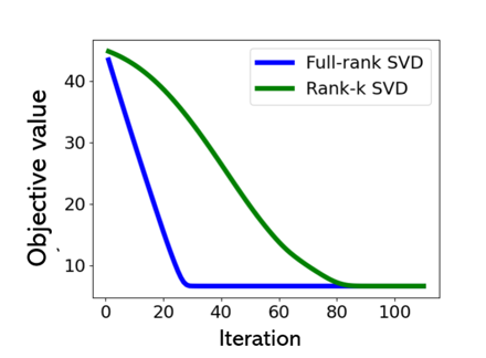
We examine the performance of nonconvex PGD over 𝒫n,k\mathcal{P}_{n,k} (Dynamics (2)) for the spiked covariance model considered above, but this time, when initialized with a random (uniformly distributed) projection matrix. We compare it with convex PGD which optimizes over the Fantope ℱn,k\mathcal{F}_{n,k} and uses a full-rank SVD to compute the projection. We use the same step-size as before. We see in Figure 2 (right panel) two trends. First, we clearly see that PGD w.r.t. 𝒫n,k\mathcal{P}_{n,k} and ℱn,k\mathcal{F}_{n,k} produce very different iterates which in particular implies that, as opposed to the case of warm-start initializaion, the projections of convex PGD onto the Fantope, throughout most of the run are not rank-kk. Second, we see that nonconvex PGD is significantly slower than convex PGD. Thus, while both methods eventually converge to the same error, this suggests that far from a global minimizer, the behaviour of nonconvex gradient methods is indeed significantly different than in the local proximity of one, which supports the fact that our theoretical guarantees only hold in a local neighbourhood of a minimizer.

Refer to caption
Refer to caption
Figure 2: Convergence of PGD for the spiked covariance model with p=0.1p=0.1 over the Fantope ℱn,k\mathcal{F}_{n,k} with a full-rank SVD, and over 𝒫n,k\mathcal{P}_{n,k} with rank-kk SVD, when initialized with the PCA solution (left panel) and with random initialization (right panel). In the left panel the plots exactly coincide.

References

  • [1] Farid Alizadeh, Jean-Pierre A Haeberly, and Michael L Overton. Complementarity and nondegeneracy in semidefinite programming. Mathematical programming, 77(1):111–128, 1997.
  • [2] Srinadh Bhojanapalli, Anastasios Kyrillidis, and Sujay Sanghavi. Dropping convexity for faster semi-definite optimization. In Vitaly Feldman, Alexander Rakhlin, and Ohad Shamir, editors, 29th Annual Conference on Learning Theory, volume 49 of Proceedings of Machine Learning Research, pages 530–582, Columbia University, New York, New York, USA, 23–26 Jun 2016. PMLR.
  • [3] Sébastien Bubeck. Convex optimization: Algorithms and complexity. arXiv preprint arXiv:1405.4980, 2014.
  • [4] Yudong Chen and Martin J Wainwright. Fast low-rank estimation by projected gradient descent: General statistical and algorithmic guarantees. arXiv preprint arXiv:1509.03025, 2015.
  • [5] Lijun Ding, Yingjie Fei, Qiantong Xu, and Chengrun Yang. Spectral frank-wolfe algorithm: Strict complementarity and linear convergence. In International Conference on Machine Learning, pages 2535–2544. PMLR, 2020.
  • [6] Dmitriy Drusvyatskiy and Adrian S Lewis. Error bounds, quadratic growth, and linear convergence of proximal methods. Mathematics of Operations Research, 43(3):919–948, 2018.
  • [7] Ky Fan. On a theorem of weyl concerning eigenvalues of linear transformations i. Proceedings of the National Academy of Sciences of the United States of America, 35(11):652, 1949.
  • [8] Dan Garber. Linear convergence of frank-wolfe for rank-one matrix recovery without strong convexity. arXiv preprint arXiv:1912.01467, 2019.
  • [9] Dan Garber. On the convergence of projected-gradient methods with low-rank projections for smooth convex minimization over trace-norm balls and related problems. SIAM Journal on Optimization, 31(1):727–753, 2021.
  • [10] Gene H Golub and Charles F Van Loan. Matrix computations. johns hopkins studies in the mathematical sciences.
  • [11] Moritz Hardt and Ankur Moitra. Algorithms and hardness for robust subspace recovery. In Conference on Learning Theory, pages 354–375. PMLR, 2013.
  • [12] Martin Jaggi. Revisiting frank-wolfe: Projection-free sparse convex optimization. In International Conference on Machine Learning, pages 427–435. PMLR, 2013.
  • [13] Atara Kaplan and Dan Garber. Low-rank extragradient method for nonsmooth and low-rank matrix optimization problems. Advances in Neural Information Processing Systems, 34, 2021.
  • [14] Hamed Karimi, Julie Nutini, and Mark Schmidt. Linear convergence of gradient and proximal-gradient methods under the polyak-łojasiewicz condition. In Joint European Conference on Machine Learning and Knowledge Discovery in Databases, pages 795–811. Springer, 2016.
  • [15] Andrew J Landgraf and Yoonkyung Lee. Dimensionality reduction for binary data through the projection of natural parameters. Journal of Multivariate Analysis, 180:104668, 2020.
  • [16] Gilad Lerman and Tyler Maunu. Fast, robust and non-convex subspace recovery. Information and Inference: A Journal of the IMA, 7(2):277–336, 2018.
  • [17] Gilad Lerman and Tyler Maunu. An overview of robust subspace recovery. Proceedings of the IEEE, 106(8):1380–1410, 2018.
  • [18] Tyler Maunu, Teng Zhang, and Gilad Lerman. A well-tempered landscape for non-convex robust subspace recovery. Journal of Machine Learning Research, 20(37), 2019.
  • [19] Ion Necoara, Yu Nesterov, and Francois Glineur. Linear convergence of first order methods for non-strongly convex optimization. Mathematical Programming, 175(1):69–107, 2019.
  • [20] Michael L Overton and Robert S Womersley. On the sum of the largest eigenvalues of a symmetric matrix. SIAM Journal on Matrix Analysis and Applications, 13(1):41–45, 1992.
  • [21] Dohyung Park, Anastasios Kyrillidis, Constantine Caramanis, and Sujay Sanghavi. Finding low-rank solutions via nonconvex matrix factorization, efficiently and provably. SIAM Journal on Imaging Sciences, 11(4):2165–2204, 2018.
  • [22] Prasad Raghavendra and Morris Yau. List decodable subspace recovery. In Conference on Learning Theory, pages 3206–3226. PMLR, 2020.
  • [23] Mostafa Rahmani and George K Atia. Randomized robust subspace recovery and outlier detection for high dimensional data matrices. IEEE Transactions on Signal Processing, 65(6):1580–1594, 2016.
  • [24] Yousef Saad. Numerical methods for large eigenvalue problems: revised edition. SIAM, 2011.
  • [25] Ohad Shamir. Fast stochastic algorithms for svd and pca: Convergence properties and convexity. In International Conference on Machine Learning, pages 248–256. PMLR, 2016.
  • [26] Vincent Q Vu, Juhee Cho, Jing Lei, and Karl Rohe. Fantope projection and selection: A near-optimal convex relaxation of sparse pca. Advances in neural information processing systems, 26, 2013.
  • [27] Yi Yu, Tengyao Wang, and Richard J Samworth. A useful variant of the davis–kahan theorem for statisticians. Biometrika, 102(2):315–323, 2015.
  • [28] Dejiao Zhang and Laura Balzano. Global convergence of a grassmannian gradient descent algorithm for subspace estimation. In Artificial Intelligence and Statistics, pages 1460–1468. PMLR, 2016.
  • [29] Zirui Zhou and Anthony Man-Cho So. A unified approach to error bounds for structured convex optimization problems. Mathematical Programming, 165(2):689–728, 2017.

Appendix A Additional Details on Experiments

The first robust recovery model we consider is a spiked covariance model, in which we draw a uniformly distributed projection matrix onto a kk-dimensional subspace 𝐏∈𝒫n,k{\mathbf{P}}\in\mathcal{P}_{n,k}, and we generate mm samples 𝐪1,…,𝐪m∈ℝn{\mathbf{q}}_{1},\dots,{\mathbf{q}}_{m}\in\mathbb{R}^{n} such that for each i∈[m]i\in[m], we set 𝐪i=𝐏𝐳i/‖𝐏𝐳i‖{\mathbf{q}}_{i}={\mathbf{P}}{\mathbf{z}}_{i}/\|{{\mathbf{P}}{\mathbf{z}}_{i}}\| with probability 1−p1-p, and 𝐪i=𝐳i{\mathbf{q}}_{i}={\mathbf{z}}_{i} with probability pp, where p∈(0,0.5]p\in(0,0.5], and 𝐳1,…,𝐳m{\mathbf{z}}_{1},\dots,{\mathbf{z}}_{m} are i.i.d. uniformly distributed unit vectors. The goal is to recover 𝐏{\mathbf{P}} by minimizing the following objective function over ℱn,k\mathcal{F}_{n,k}:

f⁡(𝐗)=∑i=1mHuberγ​(‖𝐪i−a​𝐗𝐪i‖),Huberγ​(x):={12​x2if |x|≤γγ⁡(|x|−12​γ)else.\displaystyle f({\mathbf{X}})=\sum_{i=1}^{m}\textrm{Huber}_{\gamma}(\|{\mathbf{q}}_{i}-a{\mathbf{X}}{\mathbf{q}}_{i}\|),\quad\textrm{Huber}_{\gamma}(x):=\begin{cases}\frac{1}{2}x^{2}&\text{if $|x|\leq\gamma$}\\ \gamma(|x|-\frac{1}{2}\gamma)&\text{else}.\end{cases}

Here a∈(0,1]a\in(0,1] is a regularization parameter and we set it to slightly less than one.

The second model we consider is that of sparsely corrupted entries in which we again draw a uniformly distributed projection matrix 𝐏{\mathbf{P}}. This time the data points 𝐪1,…,𝐪m{\mathbf{q}}_{1},\dots,{\mathbf{q}}_{m} are generated by taking 𝐪i=𝐏𝐳i/‖𝐏𝐳i‖{\mathbf{q}}_{i}={\mathbf{P}}{\mathbf{z}}_{i}/\|{{\mathbf{P}}{\mathbf{z}}_{i}}\| for each i∈[m]i\in[m], where as before 𝐳1,…,𝐳m{\mathbf{z}}_{1},\dots,{\mathbf{z}}_{m} are i.i.d. uniformly distributed unit vectors, but for each i∈[m]i\in[m], with probability pp, we pick a uniformly distributed entry j∈[n]j\in[n] and set it to −1-1 or +1+1 (with equal probability). The goal is to recover 𝐏{\mathbf{P}} by minimizing the following objective function over ℱn,k\mathcal{F}_{n,k}:

f⁡(𝐗)=∑i=1m∑j=1nHuberγ​([𝐪i]j−[a​𝐗𝐪i]j),\displaystyle f({\mathbf{X}})=\sum_{i=1}^{m}\sum_{j=1}^{n}\textrm{Huber}_{\gamma}([{\mathbf{q}}_{i}]_{j}-[a{\mathbf{X}}{\mathbf{q}}_{i}]_{j}),

where here also a∈(0,1]a\in(0,1] is a regularization parameter.

For both models we set the Huber loss parameter to γ=0.1\gamma=0.1. For the first model we set a=0.9a=0.9 and for the second a=0.8a=0.8. For a given projection matrix 𝐗∈𝒫n,k{\mathbf{X}}\in\mathcal{P}_{n,k}, we measure the recovery error according to ‖𝐗−𝐏‖F2\|{{\mathbf{X}}-{\mathbf{P}}}\|_{F}^{2}. For both models we let 𝐗P​C​A∈𝒫n,k{\mathbf{X}}_{PCA}\in\mathcal{P}_{n,k} denote the standard PCA solution, i.e., the projection matrix onto the span of the top kk eigenvectors of the empirical covariance 1m​∑i=1m𝐪i​𝐪i⊤\frac{1}{m}\sum_{i=1}^{m}{\mathbf{q}}_{i}{\mathbf{q}}_{i}^{\top}. For both models we set n=100n=100, k=10k=10, and m=500m=500. For both models we use the projected gradient method to find a projection matrix 𝐗∗∈𝒫n,k{\mathbf{X}}^{*}\in\mathcal{P}_{n,k} which has negligible dual gap (<10−10<10^{-10}). 33 3 For 𝐗∈ℱn,k{\mathbf{X}}\in\mathcal{F}_{n,k} the dual gap is defined as dg​(𝐗)=⟨𝐗−𝐕,∇f​(𝐗)⟩\textrm{dg}({\mathbf{X}})=\langle{{\mathbf{X}}-{\mathbf{V}},\nabla{}f({\mathbf{X}})}\rangle, were 𝐕∈arg​min𝐙∈𝒫n,k⁡⟨𝐙,∇f​(𝐗)⟩{\mathbf{V}}\in\argmin_{{\mathbf{Z}}\in\mathcal{P}_{n,k}}\langle{{\mathbf{Z}},\nabla{}f({\mathbf{X}})}\rangle. Since f⁡(⋅)f(\cdot) is convex, we in particular have f⁡(𝐗)−min𝐘∈ℱn,k⁡f⁡(𝐘)≤dg​(𝐗)f({\mathbf{X}})-\min_{{\mathbf{Y}}\in\mathcal{F}_{n,k}}f({\mathbf{Y}})\leq\textrm{dg}({\mathbf{X}}). For this 𝐗∗{\mathbf{X}}^{*} we measure the corresponding eigen-gap λn−k​(∇f​(𝐗∗))−λn−k+1​(∇f​(𝐗∗))\lambda_{n-k}(\nabla{}f({\mathbf{X}}^{*}))-\lambda_{n-k+1}(\nabla{}f({\mathbf{X}}^{*})), and the recovery error ‖𝐗∗−𝐏‖F\|{{\mathbf{X}}^{*}-{\mathbf{P}}}\|_{F}. The results are given in Table 1. For each set of parameters the results are the average of 20 i.i.d. experiments.

Refer to caption
Refer to caption
Refer to caption
Refer to caption
Figure 3: Convergence of PGD and GOI for the sparsely corrupted entries model with p=0.1p=0.1. 1st and 3rd panels from the left show the recovery error (𝐏{\mathbf{P}} is the ground truth projection matrix) and approximation error w.r.t. objective value of PGD, respectively. Convergence of GOI is omitted since it coincides with that of PGD. 2nd panel from the left shows the distance (in Frobenius norm) between the iterates of PGD (𝐗t)({\mathbf{X}}_{t}) and those of GOI (𝐘t)({\mathbf{Y}}_{t}). The rightmost panel shows the approximation error (in log scale) vs. time, when only the time to compute matrix factorizations is taken into account.

In a second experiment we fix for both models p=0.1p=0.1 and vary the dimension nn (while keeping k,mk,m fixed as before). The results are given in Table 2. In particular, we see that the eigen-gap δ\delta does not change substantially with the dimension.

dim. (nn) 100 200 300 400
↓\downarrow Model 1: spiked covariance ↓\downarrow
Eigen-gap (δ\delta) 2.87 3.02 2.96 3.04
‖𝐗∗−𝐏‖F\|{\mathbf{X}}^{*}-{\mathbf{P}}\|_{F} 0.00710.0071 0.0050.005 0.00430.0043 0.00350.0035
‖𝐗P​C​A−𝐏‖F\|{\mathbf{X}}_{PCA}-{\mathbf{P}}\|_{F} 0.068 0.049 0.043 0.036
↓\downarrow Model 2: sparsely corrupted entries ↓\downarrow
Eigen-gap (δ\delta) 5.49 5.902 6.06 6.1
‖𝐗∗−𝐏‖F\|{\mathbf{X}}^{*}-{\mathbf{P}}\|_{F} 0.0670.067 0.06170.0617 0.0580.058 0.0550.055
‖𝐗P​C​A−𝐏‖F\|{\mathbf{X}}_{PCA}-{\mathbf{P}}\|_{F} 0.199 0.208 0.206 0.202
Table 2: Recovery and eigen-gap results for the spiked covariance model and corrupted entries model with varying dimension. Each result is the average of 20 i.i.d. experiments.

We turn to demonstrate the empirical performance of the projected gradient method w.r.t. to the nonconvex set 𝒫n,k\mathcal{P}_{n,k} (PGD), as given in Dynamics (2), and and gradient orthogonal iteration (GOI), as given in Dynamics (1), for the two models discussed above. We fix n=100n=100 and p=0.1p=0.1 (keeping all other parameters unchanged). For both methods we use the fixed step-size η=1/λ\eta=1/\lambda, where λ=λ1​(∑i=1m𝐪i​𝐪i⊤)\lambda=\lambda_{1}(\sum_{i=1}^{m}{\mathbf{q}}_{i}{\mathbf{q}}_{i}^{\top}), i.e., the largest eigenvalue of the (unnormalized) empirical covariance. We note that smaller values of η\eta seem too conservative in practice from our experimentations. We initialize both methods with the kk-PCA projection matrix 𝐗P​C​A{\mathbf{X}}_{PCA}. We examine the convergence of both methods in terms of recovery error and approximation error (w.r.t. the objective function). Additionally, to showcase the benefit of avoiding exact SVD computations (as employed by nonconvex PGD) and using only a single QR factorization per iteration (as in GOI), we compare the runtimes of GOI and nonconvex PGD, but we exclude the time it takes to compute the gradient on each iteration and only account for the time it takes to perform either a rank−k\textrm{rank}-k SVD or a QR factorization, where both algorithms were implemented in Python and we have used the built-in functions numpy.linalg.eigh and numpy.linalg.qr to compute thin-SVDs and QR factorizations, respectively.

The results for the spiked covariance model are given in Figure 1, and the results for the sparsely corrupted entries model, which are very similar, are given in Figure 3. It can be seen that indeed the distance between the iterates of the two methods decays very quickly and so the graphs of the recovery and approximation errors of both methods coincide. We in particular see that both methods indeed demonstrate a linear convergence rate (w.r.t. the objective value). We also see the significant savings in runtime when replacing a thin-SVD computation (as used by nonconvex PGD) with only a single QR factorization (as used by GOI).

Moreover, in order to verify the convergence of nonconvex PGD to the global optimal solution (and not just a stationary point of the nonconvex Problem (1)), we verify using the procedure suggested in Remark 3, that on each iteration tt, the projection step onto the Fantope ℱn,k\mathcal{F}_{n,k} is also of rank kk, i.e., identical to the projection onto 𝒫n,k\mathcal{P}_{n,k}. This means that the iterates of PGD w.r.t. the nonconvex Problem (1) and the iterates of PGD w.r.t. the convex relaxation (4), coincide. Indeed, for all random instances generated and for all iterations executed, we observe that the projection onto the Fantope is of rank kk. This suggests that the nonconvex PGD (and consequently also GOI) in particular converges to the global optimal solution of the convex relaxation (4).

Appendix B Proof of Theorem 2

Proof.

First, observe that for any dual solution (𝐙1∗,𝐙2∗,s∗)({\mathbf{Z}}_{1}^{*},{\mathbf{Z}}_{2}^{*},s^{*}), it holds that 𝐙1∗{\mathbf{Z}}_{1}^{*} and 𝐙2∗{\mathbf{Z}}_{2}^{*} are orthogonal to each other. This is true since, denoting by 𝐗∗{\mathbf{X}}^{*} the corresponding primal solution, we have that,

⟨𝐙1∗,𝐙2∗⟩\displaystyle\langle{\mathbf{Z}}_{1}^{*},{\mathbf{Z}}_{2}^{*}\rangle =Tr​(𝐙1∗​𝐙2∗)=Tr​(𝐙1∗​(𝐗∗+(𝐈−𝐗∗))​𝐙2∗)\displaystyle=\textrm{Tr}({\mathbf{Z}}_{1}^{*}{\mathbf{Z}}_{2}^{*})=\textrm{Tr}({\mathbf{Z}}_{1}^{*}({\mathbf{X}}^{*}+({\mathbf{I}}-{\mathbf{X}}^{*})){\mathbf{Z}}_{2}^{*})
=Tr​(𝐙1∗​𝐗∗​𝐙2∗)+Tr​(𝐙1∗​(𝐈−𝐗∗)​𝐙2∗)=0,\displaystyle=\textrm{Tr}({\mathbf{Z}}_{1}^{*}{\mathbf{X}}^{*}{\mathbf{Z}}_{2}^{*})+\textrm{Tr}({\mathbf{Z}}_{1}^{*}({\mathbf{I}}-{\mathbf{X}}^{*}){\mathbf{Z}}_{2}^{*})=0,

where the last equality follows from the complementarity conditions 𝐙1∗​𝐗∗=𝟎{\mathbf{Z}}_{1}^{*}{\mathbf{X}}^{*}=\mathbf{0} and (𝐈−𝐗∗)​𝐙2∗=𝟎({\mathbf{I}}-{\mathbf{X}}^{*}){\mathbf{Z}}_{2}^{*}=\mathbf{0}.

For a given dual solution (𝐙1∗,𝐙2∗,s∗)({\mathbf{Z}}_{1}^{*},{\mathbf{Z}}_{2}^{*},s^{*}), let us denote r1=rank​(𝐙1∗)r_{1}=\textrm{rank}({\mathbf{Z}}_{1}^{*}) and r2=rank​(𝐙2∗)r_{2}=\textrm{rank}({\mathbf{Z}}_{2}^{*}).

Let us write the eigen decompositions 𝐙1∗=∑i=1r1ρi​𝐮i​𝐮iT{\mathbf{Z}}_{1}^{*}=\sum_{i=1}^{r_{1}}\rho_{i}{\mathbf{u}}_{i}{\mathbf{u}}_{i}^{T} and 𝐙2∗=∑j=1r2μj​𝐯j​𝐯jT{\mathbf{Z}}_{2}^{*}=\sum_{j=1}^{r_{2}}\mu_{j}{\mathbf{v}}_{j}{\mathbf{v}}_{j}^{T}.

From the orthogonality of 𝐙1∗{\mathbf{Z}}_{1}^{*} and 𝐙2∗{\mathbf{Z}}_{2}^{*} established above, we get an orthonormal set of vectors {𝐮1,…,𝐮r1,𝐯1,…,𝐯r2}\{{\mathbf{u}}_{1},...,{\mathbf{u}}_{r_{1}},{\mathbf{v}}_{1},...,{\mathbf{v}}_{r_{2}}\} and we can complete it to an orthonormal basis of ℝn\mathbb{R}^{n}:

B={𝐮1,…,𝐮r1,𝐯1,…,𝐯r2,𝐰1,…,𝐰n−r1−r2},\displaystyle B=\{{\mathbf{u}}_{1},...,{\mathbf{u}}_{r_{1}},{\mathbf{v}}_{1},...,{\mathbf{v}}_{r_{2}},{\mathbf{w}}_{1},...,{\mathbf{w}}_{n-r_{1}-r_{2}}\},

where 𝐙1∗​𝐰i=𝟎{\mathbf{Z}}_{1}^{*}{\mathbf{w}}_{i}=\mathbf{0} and 𝐙2∗​𝐰i=𝟎{\mathbf{Z}}_{2}^{*}{\mathbf{w}}_{i}=\mathbf{0} for any i∈{1,…,n−r1−r2}i\in\{1,\dots,n-r_{1}-r_{2}\}.

From the KKT conditions for Problem (4), we have that ∇f​(𝐗∗)=𝐙1∗−𝐙2∗+s∗​𝐈\nabla f({\mathbf{X}}^{*})={\mathbf{Z}}_{1}^{*}-{\mathbf{Z}}_{2}^{*}+s^{*}{\mathbf{I}}, and so it follows that any 𝐯∈B{\mathbf{v}}\in B is an eigenvector of ∇f​(𝐗∗)\nabla f({\mathbf{X}}^{*}). Thus, we can write the eigenvalues of ∇f​(𝐗∗)\nabla f({\mathbf{X}}^{*}) in non-increasing order from left to right as:

ρ1+s∗,…,ρr1+s∗,s∗,…,s∗⏟n−r1−r2​times,s∗−μr2,…,s∗−μ1.\displaystyle\rho_{1}+s^{*},...,\rho_{r_{1}}+s^{*},\underbrace{s^{*},...,s^{*}}_{n-r_{1}-r_{2}~\textrm{times}},s^{*}-\mu_{r_{2}},...,s^{*}-\mu_{1}. (17)

For the first direction of the theorem, let us assume 𝐗∗{\mathbf{X}}^{*} satisfies strict complementarity, so for some dual solution (𝐙1∗,𝐙2∗,s∗)({\mathbf{Z}}_{1}^{*},{\mathbf{Z}}_{2}^{*},s^{*}) we have that r1=n−kr_{1}=n-k or r2=kr_{2}=k.

Now, if r1=n−kr_{1}=n-k, using (17) we get that λn−k​(∇f​(𝐗∗))=ρn−k+s∗\lambda_{n-k}(\nabla f({\mathbf{X}}^{*}))=\rho_{n-k}+s^{*} and
λn−k+1​(∇f​(𝐗∗))≤s∗\lambda_{n-k+1}(\nabla f({\mathbf{X}}^{*}))\leq s^{*}, and so there is a gap of

λn−k​(∇f​(𝐗∗))−λn−k+1​(∇f​(𝐗∗))≥ρn−k+s∗−s∗=ρn−k>0.\displaystyle\lambda_{n-k}(\nabla f({\mathbf{X}}^{*}))-\lambda_{n-k+1}(\nabla f({\mathbf{X}}^{*}))\geq\rho_{n-k}+s^{*}-s^{*}=\rho_{n-k}>0.

Otherwise, if r2=kr_{2}=k, then using (17) we have that λn−k+1​(∇f​(𝐗∗))=s∗−μk\lambda_{n-k+1}(\nabla f({\mathbf{X}}^{*}))=s^{*}-\mu_{k} and
λn−k​(∇f​(𝐗∗))>s∗\lambda_{n-k}(\nabla f({\mathbf{X}}^{*}))>s^{*}, and so there is a gap of

λn−k​(∇f​(𝐗∗))−λn−k+1​(∇f​(𝐗∗))≥s∗−(s∗−μk)=μk>0.\displaystyle\lambda_{n-k}(\nabla f({\mathbf{X}}^{*}))-\lambda_{n-k+1}(\nabla f({\mathbf{X}}^{*}))\geq s^{*}-(s^{*}-\mu_{k})=\mu_{k}>0.

In both cases we get a positive eigen-gap, which proves the first direction of the theorem.

For the reversed direction, let us assume that 𝐗∗{\mathbf{X}}^{*} satisfies the eigen-gap assumption, and recall that according to Theorem 1 it follows that rank​(𝐗∗)=k\textrm{rank}({\mathbf{X}}^{*})=k. Suppose by way of contradiction that there exists a dual solution (𝐙1∗,𝐙2∗,s∗)({\mathbf{Z}}_{1}^{*},{\mathbf{Z}}_{2}^{*},s^{*}) for which r1<n−kr_{1}<n-k and r2<kr_{2}<k. In this case we have from (17) that,

λn−k​(∇f​(𝐗∗))=λn−k+1​(∇f​(𝐗∗))=s∗,\displaystyle\lambda_{n-k}(\nabla f({\mathbf{X}}^{*}))=\lambda_{n-k+1}(\nabla f({\mathbf{X}}^{*}))=s^{*},

which contradicts the existence of an eigen-gap and so, it must be that r1=n−kr_{1}=n-k or r2=kr_{2}=k. ∎

Appendix C Details Missing from Section 3.1 and Proof of Theorem 1

C.1 Proof of Lemma 1

Proof.

The first part of the lemma is a known fact, see for instance [26]. For the second part, let us prove that if ∑i=1rmin⁡(γi−γr+1,1)≥k\sum_{i=1}^{r}\min(\gamma_{i}-\gamma_{r+1},1)\geq k, then θ\theta must satisfy θ≥γr+1\theta\geq\gamma_{r+1}. Assume by way contradiction that θ<γr+1\theta<\gamma_{r+1}. Then,

k=∑i=1nmin⁡(max⁡(γi−θ,0),1)>∑i=1nmin⁡(max⁡(γi−γr+1,0),1)=∑i=1rmin⁡(γi−γr+1,1),\displaystyle k=\sum_{i=1}^{n}\min(\max(\gamma_{i}-\theta,0),1)>\sum_{i=1}^{n}\min(\max(\gamma_{i}-\gamma_{r+1},0),1)=\sum_{i=1}^{r}\min(\gamma_{i}-\gamma_{r+1},1),

which is a contradiction, and so it must be that θ≥γr+1\theta\geq\gamma_{r+1}, and in that case the projection sets all the bottom n−rn-r components of the eigen-decomposition of 𝐗{\mathbf{X}} to zero. Hence, rank​(Πℱn,k​[𝐗])≤r\textrm{rank}(\Pi_{\mathcal{F}_{n,k}}[{\mathbf{X}}])\leq r. The reversed direction holds from similar reasoning. ∎

C.2 Proof of Theorem 1

Before we prove Theorem 1 we need the following lemma which is central to our analysis and connects between an optimal solution and the eigen-decomposition of its corresponding gradient.

Lemma 6.

Let 𝐗∗∈ℱn,k{\mathbf{X}}^{*}\in\mathcal{F}_{n,k} be an optimal solution to Problem (4) and write the eigen-
decomposition of −∇f​(𝐗∗)-\nabla f({\mathbf{X}}^{*}) as −∇f​(𝐗∗)=∑i=1nμi​𝐮i​𝐮i⊤-\nabla f({\mathbf{X}}^{*})=\sum_{i=1}^{n}\mu_{i}{\mathbf{u}}_{i}{\mathbf{u}}_{i}^{\top}. Let rr be the smallest integer such that r≥kr\geq k and μk−μr+1>0\mu_{k}-\mu_{r+1}>0. Then, for all n≥i≥r+1n\geq i\geq r+1, 𝐗∗{\mathbf{X}}^{*} is orthogonal to 𝐮i​𝐮i⊤{\mathbf{u}}_{i}{\mathbf{u}}_{i}^{\top}, and rank​(𝐗∗)≤r\textrm{rank}({\mathbf{X}}^{*})\leq r.
In particular, if r=kr=k, then 𝐗∗∈𝒫n,k{\mathbf{X}}^{*}\in\mathcal{P}_{n,k} is the unique projection matrix onto the span of the kk leading eigenvectors of −∇f​(𝐗∗)-\nabla f({\mathbf{X}}^{*}).

Proof.

Assume by way of contradiction that 𝐗∗{\mathbf{X}}^{*} is not orthogonal 𝐮r+1​𝐮r+1⊤,…,𝐮n​𝐮n⊤{\mathbf{u}}_{r+1}{\mathbf{u}}_{r+1}^{\top},\dots,{\mathbf{u}}_{n}{\mathbf{u}}_{n}^{\top}. In this case, ∑i=r+1n𝐮i⊤​𝐗∗​𝐮i>0\sum_{i=r+1}^{n}{\mathbf{u}}_{i}^{\top}{\mathbf{X}}^{*}{\mathbf{u}}_{i}>0, and we can write,

⟨𝐗∗,−∇f​(𝐗∗)⟩\displaystyle\langle{\mathbf{X}}^{*},-\nabla f({\mathbf{X}}^{*})\rangle =∑i=1rμi​𝐮i⊤​𝐗∗​𝐮i+∑i=r+1nμi​𝐮i⊤​𝐗∗​𝐮i\displaystyle=\sum_{i=1}^{r}\mu_{i}{\mathbf{u}}_{i}^{\top}{\mathbf{X}}^{*}{\mathbf{u}}_{i}+\sum_{i=r+1}^{n}\mu_{i}{\mathbf{u}}_{i}^{\top}{\mathbf{X}}^{*}{\mathbf{u}}_{i}
<(a)​∑i=1rμi​𝐮i⊤​𝐗∗​𝐮i+μr​∑i=r+1n𝐮i⊤​𝐗∗​𝐮i\displaystyle\underset{(a)}{<}\sum_{i=1}^{r}\mu_{i}{\mathbf{u}}_{i}^{\top}{\mathbf{X}}^{*}{\mathbf{u}}_{i}+\mu_{r}\sum_{i=r+1}^{n}{\mathbf{u}}_{i}^{\top}{\mathbf{X}}^{*}{\mathbf{u}}_{i}
=(b)​∑i=1k−1μi​𝐮i⊤​𝐗∗​𝐮i+μk​∑i=kn𝐮i⊤​𝐗∗​𝐮i\displaystyle\underset{(b)}{=}\sum_{i=1}^{k-1}\mu_{i}{\mathbf{u}}_{i}^{\top}{\mathbf{X}}^{*}{\mathbf{u}}_{i}+\mu_{k}\sum_{i=k}^{n}{\mathbf{u}}_{i}^{\top}{\mathbf{X}}^{*}{\mathbf{u}}_{i}
=(c)​∑i=1k−1μi​𝐮i⊤​𝐗∗​𝐮i+μk​(k−∑i=1k−1𝐮i⊤​𝐗∗​𝐮i),\displaystyle\underset{(c)}{=}\sum_{i=1}^{k-1}\mu_{i}{\mathbf{u}}_{i}^{\top}{\mathbf{X}}^{*}{\mathbf{u}}_{i}+\mu_{k}\left({k-\sum_{i=1}^{k-1}{\mathbf{u}}_{i}^{\top}{\mathbf{X}}^{*}{\mathbf{u}}_{i}}\right),

where both (a) and (b) follow from the definition of rr, and (c) follows since ∑i=1n𝐮i⊤​𝐗∗​𝐮i=Tr​(𝐗∗​∑i=1n𝐮i​𝐮i∗)=Tr​(𝐗∗​𝐈)=k\sum_{i=1}^{n}{\mathbf{u}}_{i}^{\top}{\mathbf{X}}^{*}{\mathbf{u}}_{i}=\textrm{Tr}({\mathbf{X}}^{*}\sum_{i=1}^{n}{\mathbf{u}}_{i}{\mathbf{u}}_{i}^{*})=\textrm{Tr}({\mathbf{X}}^{*}{\mathbf{I}})=k.

Let us denote the projection matrix onto the span of the top kk eigenvectors of −∇f​(𝐗∗)-\nabla{}f({\mathbf{X}}^{*}) by 𝐏∗=∑i=1k𝐮i​𝐮i⊤{\mathbf{P}}^{*}=\sum_{i=1}^{k}{\mathbf{u}}_{i}{\mathbf{u}}_{i}^{\top}, and note that ⟨𝐏∗,−∇f​(𝐗∗)⟩=∑i=1kμi\langle{{\mathbf{P}}^{*},-\nabla{}f({\mathbf{X}}^{*})}\rangle=\sum_{i=1}^{k}\mu_{i}. It follows that

⟨𝐏∗−𝐗∗,∇f​(𝐗∗)⟩\displaystyle\langle{{\mathbf{P}}^{*}-{\mathbf{X}}^{*},\nabla{}f({\mathbf{X}}^{*})}\rangle =⟨𝐗∗−𝐏∗,−∇f​(𝐗∗)⟩\displaystyle=\langle{{\mathbf{X}}^{*}-{\mathbf{P}}^{*},-\nabla{}f({\mathbf{X}}^{*})}\rangle
<∑i=1k−1μi​𝐮i⊤​𝐗∗​𝐮i+μk​(k−∑i=1k−1𝐮i⊤​𝐗∗​𝐮i)−∑i=1kμi\displaystyle<\sum_{i=1}^{k-1}\mu_{i}{\mathbf{u}}_{i}^{\top}{\mathbf{X}}^{*}{\mathbf{u}}_{i}+\mu_{k}\left({k-\sum_{i=1}^{k-1}{\mathbf{u}}_{i}^{\top}{\mathbf{X}}^{*}{\mathbf{u}}_{i}}\right)-\sum_{i=1}^{k}\mu_{i}
=∑i=1k−1μi​(𝐮i⊤​𝐗∗​𝐮i−1)+μk​∑i=1k−1(1−𝐮i⊤​𝐗∗​𝐮i)\displaystyle=\sum_{i=1}^{k-1}\mu_{i}\left({{\mathbf{u}}_{i}^{\top}{\mathbf{X}}^{*}{\mathbf{u}}_{i}-1}\right)+\mu_{k}\sum_{i=1}^{k-1}\left({1-{\mathbf{u}}_{i}^{\top}{\mathbf{X}}^{*}{\mathbf{u}}_{i}}\right)
=∑i=1k−1(1−𝐮i⊤​𝐗∗​𝐮i)​(μk−μi)≤0,\displaystyle=\sum_{i=1}^{k-1}\left(1-{{\mathbf{u}}_{i}^{\top}{\mathbf{X}}^{*}{\mathbf{u}}_{i}}\right)(\mu_{k}-\mu_{i})\leq 0,

where the last inequality follows since for all ii, 𝐮i⊤​𝐗∗​𝐮i∈[0,1]{\mathbf{u}}_{i}^{\top}{\mathbf{X}}^{*}{\mathbf{u}}_{i}\in[0,1].

Thus, we have that 𝐗∗{\mathbf{X}}^{*} violates the first-order optimality condition which contradicts that assumption that it is an optimal solution, and thus we have that 𝐗∗{\mathbf{X}}^{*} must indeed be orthogonal to 𝐮r+1​𝐮r+1⊤,…,𝐮n​𝐮n⊤{\mathbf{u}}_{r+1}{\mathbf{u}}_{r+1}^{\top},\dots,{\mathbf{u}}_{n}{\mathbf{u}}_{n}^{\top}.

An immediate consequence is that the eigenvectors of 𝐗∗{\mathbf{X}}^{*} which correspond to non-zero eigenvalues must lie in span​{𝐮1,…,𝐮r}\textrm{span}\{{\mathbf{u}}_{1},...,{\mathbf{u}}_{r}\} and thus, it must be that rank​(𝐗∗)≤r\textrm{rank}({\mathbf{X}}^{*})\leq r.

For the final part of the lemma, in case r=kr=k, since for all 𝐗∈ℱn,k{\mathbf{X}}\in\mathcal{F}_{n,k}, rank​(𝐗)≥k\textrm{rank}({\mathbf{X}})\geq k, we have that rank​(𝐗∗)=k\textrm{rank}({\mathbf{X}}^{*})=k. In particular, 𝐗∗{\mathbf{X}}^{*} is a projection matrix, i.e., 𝐗∈𝒫n,k{\mathbf{X}}\in\mathcal{P}_{n,k}. By the orthogonality result above, it follows that the eigenvectors of 𝐗∗{\mathbf{X}}^{*} lie in span​{𝐮1,…,𝐮k}\textrm{span}\{{\mathbf{u}}_{1},\dots,{\mathbf{u}}_{k}\}, which means that 𝐗∗{\mathbf{X}}^{*} is indeed the projection matrix onto span​{𝐮1,…,𝐮k}\textrm{span}\{{\mathbf{u}}_{1},\dots,{\mathbf{u}}_{k}\}, as stated in the lemma. Note that when r=kr=k, this projection matrix is indeed unique (i.e., the subspace spanned by the top kk eigenvectors of −∇f​(𝐗∗)-\nabla{}f({\mathbf{X}}^{*}) is unique). ∎

We now prove Theorem 1.

Proof of Theorem 1.

Let 𝐗∗{\mathbf{X}}^{*} be an optimal solution to the convex relaxation (4) which satisfies Assumption 1 with some δ>0\delta>0. It follows directly from Lemma 6 that rank​(𝐗∗)=k\textrm{rank}({\mathbf{X}}^{*})=k. From Lemma 6 it further follows that 𝐗∗{\mathbf{X}}^{*} is the unique projection matrix onto the span of top kk eigenvectors of −∇f​(𝐗∗)-\nabla{}f({\mathbf{X}}^{*}), i.e., it is the unique matrix in 𝐗∈𝒫n,k{\mathbf{X}}\in\mathcal{P}_{n,k} such that ⟨𝐗,−∇f​(𝐗∗)⟩=∑i=1kμi\langle{{\mathbf{X}},-\nabla{}f({\mathbf{X}}^{*})}\rangle=\sum_{i=1}^{k}\mu_{i}, where we write the eigen-decomposition of −∇f​(𝐗∗)-\nabla{}f({\mathbf{X}}^{*}) as −∇f​(𝐗∗)=∑i=1nμi​𝐮i​𝐮i⊤-\nabla{}f({\mathbf{X}}^{*})=\sum_{i=1}^{n}\mu_{i}{\mathbf{u}}_{i}{\mathbf{u}}_{i}^{\top}. From the von Neumann trace inequality it follows that for any matrix 𝐗∈𝒫n,k{\mathbf{X}}\in\mathcal{P}_{n,k} it holds that ⟨𝐗,−∇f​(𝐗∗)⟩≤∑i=1nλi​(𝐗)​μi=∑i=1kλi​(𝐗)​μi=∑i=1kμi\langle{{\mathbf{X}},-\nabla{}f({\mathbf{X}}^{*})}\rangle\leq\sum_{i=1}^{n}\lambda_{i}({\mathbf{X}})\mu_{i}=\sum_{i=1}^{k}\lambda_{i}({\mathbf{X}})\mu_{i}=\sum_{i=1}^{k}\mu_{i}. Thus, we have that for all 𝐗∈𝒫n,k∖{𝐗∗}:{\mathbf{X}}\in\mathcal{P}_{n,k}\setminus\{{\mathbf{X}}^{*}\}: ⟨𝐗−𝐗∗,∇f​(𝐗∗)⟩=⟨𝐗∗−𝐗,−∇f​(𝐗∗)⟩>0\langle{{\mathbf{X}}-{\mathbf{X}}^{*},\nabla{}f({\mathbf{X}}^{*})}\rangle=\langle{{\mathbf{X}}^{*}-{\mathbf{X}},-\nabla{}f({\mathbf{X}}^{*})}\rangle>0. Since ℱn,k=conv​{𝒫n,k}\mathcal{F}_{n,k}=\textrm{conv}\{\mathcal{P}_{n,k}\}, this further implies that for all 𝐗∈ℱn,k∖{𝐗∗}{\mathbf{X}}\in\mathcal{F}_{n,k}\setminus\{{\mathbf{X}}^{*}\}: ⟨𝐗−𝐗∗,∇f​(𝐗∗)⟩>0\langle{{\mathbf{X}}-{\mathbf{X}}^{*},\nabla{}f({\mathbf{X}}^{*})}\rangle>0. Since f⁡(⋅)f(\cdot) is convex, it further holds that for all 𝐗∈ℱn,k∖{𝐗∗}{\mathbf{X}}\in\mathcal{F}_{n,k}\setminus\{{\mathbf{X}}^{*}\}: f⁡(𝐗∗)−f⁡(𝐗)≤⟨𝐗∗−𝐗,∇f​(𝐗∗)⟩<0f({\mathbf{X}}^{*})-f({\mathbf{X}})\leq\langle{{\mathbf{X}}^{*}-{\mathbf{X}},\nabla{}f({\mathbf{X}}^{*})}\rangle<0, and thus, we conclude that 𝐗∗{\mathbf{X}}^{*} is indeed the unique optimal solution to Problem (4), which also implies that it is the unique optimal solution to Problem (1). ∎

C.3 Proof of Lemma 3

Proof.

Let us write the eigen-decomposition of the gradient ∇f​(𝐗∗)\nabla f({\mathbf{X}}^{*}) as ∇f​(𝐗∗)=∑i=1nλi​𝐮i​𝐮i⊤\nabla f({\mathbf{X}}^{*})=\sum_{i=1}^{n}\lambda_{i}{\mathbf{u}}_{i}{\mathbf{u}}_{i}^{\top}. For any 𝐗∈ℱn,k{\mathbf{X}}\in\mathcal{F}_{n,k} it holds that:

f⁡(𝐗)−f⁡(𝐗∗)\displaystyle f({\mathbf{X}})-f({\mathbf{X}}^{*}) ≥(a)​⟨𝐗−𝐗∗,∇f​(𝐗∗)⟩​=(b)​∑i=1nλi​𝐮i⊤​𝐗𝐮i−∑i=n−k+1nλi\displaystyle\underset{(a)}{\geq}\langle{\mathbf{X}}-{\mathbf{X}}^{*},\nabla f({\mathbf{X}}^{*})\rangle\underset{(b)}{=}\sum_{i=1}^{n}\lambda_{i}{\mathbf{u}}_{i}^{\top}{\mathbf{X}}{\mathbf{u}}_{i}-\sum_{i=n-k+1}^{n}\lambda_{i}
≥(c)​(λn−k+1+δ)​∑i=1n−k𝐮i⊤​𝐗𝐮i+∑i=n−k+1nλi​𝐮i⊤​𝐗𝐮i−∑i=n−k+1nλi\displaystyle\underset{(c)}{\geq}(\lambda_{n-k+1}+\delta)\sum_{i=1}^{n-k}{\mathbf{u}}_{i}^{\top}{\mathbf{X}}{\mathbf{u}}_{i}+\sum_{i=n-k+1}^{n}\lambda_{i}{\mathbf{u}}_{i}^{\top}{\mathbf{X}}{\mathbf{u}}_{i}-\sum_{i=n-k+1}^{n}\lambda_{i}
=(λn−k+1+δ)​∑i=1n−k𝐮i⊤​𝐗𝐮i−∑i=n−k+1nλi​(1−𝐮i⊤​𝐗𝐮i)\displaystyle=(\lambda_{n-k+1}+\delta)\sum_{i=1}^{n-k}{\mathbf{u}}_{i}^{\top}{\mathbf{X}}{\mathbf{u}}_{i}-\sum_{i=n-k+1}^{n}\lambda_{i}(1-{\mathbf{u}}_{i}^{\top}{\mathbf{X}}{\mathbf{u}}_{i})
≥(d)​(λn−k+1+δ)​∑i=1n−k𝐮i⊤​𝐗𝐮i−λn−k+1​∑i=n−k+1n(1−𝐮i⊤​𝐗𝐮i)\displaystyle\underset{(d)}{\geq}(\lambda_{n-k+1}+\delta)\sum_{i=1}^{n-k}{\mathbf{u}}_{i}^{\top}{\mathbf{X}}{\mathbf{u}}_{i}-\lambda_{n-k+1}\sum_{i=n-k+1}^{n}(1-{\mathbf{u}}_{i}^{\top}{\mathbf{X}}{\mathbf{u}}_{i})
=λn−k+1​∑i=1n𝐮i⊤​𝐗𝐮i−k​λn−k+1+δ​∑i=1n−k𝐮i⊤​𝐗𝐮i,\displaystyle=\lambda_{n-k+1}\sum_{i=1}^{n}{\mathbf{u}}_{i}^{\top}{\mathbf{X}}{\mathbf{u}}_{i}-k\lambda_{n-k+1}+\delta\sum_{i=1}^{n-k}{\mathbf{u}}_{i}^{\top}{\mathbf{X}}{\mathbf{u}}_{i}, (18)

where (a) follows from the convexity of f⁡(𝐗)f({\mathbf{X}}), (b) follows since according Lemma 6 𝐗∗=∑i=n−k+1n𝐮i​𝐮i⊤{\mathbf{X}}^{*}=\sum_{i=n-k+1}^{n}{\mathbf{u}}_{i}{\mathbf{u}}_{i}^{\top} and so, ⟨𝐗∗,∇f​(𝐗∗)⟩=∑i=n−k+1nλi\langle{{\mathbf{X}}^{*},\nabla{}f({\mathbf{X}}^{*})}\rangle=\sum_{i=n-k+1}^{n}\lambda_{i}, (c) follows from Assumption 1, and (d) follows since 𝐗⪯𝐈{\mathbf{X}}\preceq{\mathbf{I}}, which implies that 𝐮i⊤​𝐗𝐮i≤𝐮i⊤​𝐮i=1{\mathbf{u}}_{i}^{\top}{\mathbf{X}}{\mathbf{u}}_{i}\leq{\mathbf{u}}_{i}^{\top}{\mathbf{u}}_{i}=1.

Using ∑i=1n𝐮i⊤​𝐗𝐮i=Tr​(𝐗​∑i=1n𝐮i​𝐮i⊤)=Tr​(𝐗𝐈)=k\sum_{i=1}^{n}{\mathbf{u}}_{i}^{\top}{\mathbf{X}}{\mathbf{u}}_{i}=\textrm{Tr}({\mathbf{X}}\sum_{i=1}^{n}{\mathbf{u}}_{i}{\mathbf{u}}_{i}^{\top})=\textrm{Tr}({\mathbf{X}}{\mathbf{I}})=k and Eq. (C.3), we have,

f⁡(𝐗)−f⁡(𝐗∗)≥δ​∑i=1n−k𝐮i⊤​𝐗𝐮i=δ⁡(k−∑i=n−k+1n𝐮i⊤​𝐗𝐮i).\displaystyle f({\mathbf{X}})-f({\mathbf{X}}^{*})\geq\delta\sum_{i=1}^{n-k}{\mathbf{u}}_{i}^{\top}{\mathbf{X}}{\mathbf{u}}_{i}=\delta\left({k-\sum_{i=n-k+1}^{n}{\mathbf{u}}_{i}^{\top}{\mathbf{X}}{\mathbf{u}}_{i}}\right). (19)

Also, using again the fact that 𝐗∗=∑i=n−k+1n𝐮i​𝐮i⊤{\mathbf{X}}^{*}=\sum_{i=n-k+1}^{n}{\mathbf{u}}_{i}{\mathbf{u}}_{i}^{\top}, we have that,

‖𝐗−𝐗∗‖F2=‖𝐗‖F2+‖𝐗∗‖F2−2​∑i=n−k+1n𝐮i⊤​𝐗𝐮i≤2​(k−∑i=n−k+1n𝐮i⊤​𝐗𝐮i),\displaystyle\|{\mathbf{X}}-{\mathbf{X}}^{*}\|_{F}^{2}=\|{\mathbf{X}}\|_{F}^{2}+\|{\mathbf{X}}^{*}\|_{F}^{2}-2\sum_{i=n-k+1}^{n}{\mathbf{u}}_{i}^{\top}{\mathbf{X}}{\mathbf{u}}_{i}\leq 2\left({k-\sum_{i=n-k+1}^{n}{\mathbf{u}}_{i}^{\top}{\mathbf{X}}{\mathbf{u}}_{i}}\right), (20)

where the last inequality follows since for any 𝐗∈ℱn,k{\mathbf{X}}\in\mathcal{F}_{n,k} it holds that ‖𝐗‖F2=∑i=1nλi2​(𝐗)≤∑i=1nλi​(𝐗)=k\|{\mathbf{X}}\|_{F}^{2}=\sum_{i=1}^{n}\lambda_{i}^{2}({\mathbf{X}})\leq\sum_{i=1}^{n}\lambda_{i}({\mathbf{X}})=k. Combining Eq. (19) and (20) we finally have that,

f⁡(𝐗)−f⁡(𝐗∗)≥δ2​‖𝐗−𝐗∗‖F2.\displaystyle f({\mathbf{X}})-f({\mathbf{X}}^{*})\geq\dfrac{\delta}{2}\|{\mathbf{X}}-{\mathbf{X}}^{*}\|_{F}^{2}.

∎

Appendix D Projected Gradient Descent Analysis

In this section we turn to analyze the local convergence of the projected gradient method w.r.t. the sets 𝒫n,k\mathcal{P}_{n,k} and ℱn,k\mathcal{F}_{n,k}, and to prove Theorems 4 and 6.

We first provide the proof of Lemma 2 which is fairly simple, and then prove a more general version of the lemma, which in particular allows to relax Assumption 1.

Proof of Lemma 2.

Denote 𝐘∗=𝐗∗−η∇f(𝐗∗){\mathbf{Y}}^{*}={\mathbf{X}}^{*}-\eta\nabla f({\mathbf{X}}^{*}) and denote the eigenvalues of 𝐘∗{\mathbf{Y}}^{*} in non-increasing order σi=λi(𝐘∗),i=1,…,n\sigma_{i}=\lambda_{i}({\mathbf{Y}}^{*}),i=1,\dots,n. Denote also 𝐘=𝐗−η∇f(𝐗){\mathbf{Y}}={\mathbf{X}}-\eta\nabla f({\mathbf{X}}) with its eigenvalues γi=λi(𝐘),i=1,…,n\gamma_{i}=\lambda_{i}({\mathbf{Y}}),i=1,\dots,n. Let us write the eigen-decomposition of −∇f​(𝐗∗)-\nabla{}f({\mathbf{X}}^{*}) as −∇f​(𝐗∗)=∑i=1nμi​𝐮i​𝐮i⊤-\nabla{}f({\mathbf{X}}^{*})=\sum_{i=1}^{n}\mu_{i}{\mathbf{u}}_{i}{\mathbf{u}}_{i}^{\top}. From Lemma 6, we have that under Assumption 1, it holds that 𝐗∗=∑i=1k𝐮i​𝐮i⊤{\mathbf{X}}^{*}=\sum_{i=1}^{k}{\mathbf{u}}_{i}{\mathbf{u}}_{i}^{\top}. Thus, we can deduce that

σi={1+η​μiif i∈{1,…,k};η​μielse.\displaystyle\sigma_{i}=\begin{cases}1+\eta\mu_{i}&\text{if $i\in\{1,...,k\};$}\\ \eta\mu_{i}&\text{else.}\end{cases} (21)

From Lemma 1 we have that rank​(Πℱn,k​(𝐘))=k\textrm{rank}(\Pi_{\mathcal{F}_{n,k}}({\mathbf{Y}}))=k if and only if ∑i=1kmin⁡(γi−γk+1,1)≥k\sum_{i=1}^{k}\min(\gamma_{i}-\gamma_{k+1},1)\geq k. Thus, a sufficient condition so that rank​(Πℱn,k​(𝐘))=k\textrm{rank}(\Pi_{\mathcal{F}_{n,k}}({\mathbf{Y}}))=k is,

γk−γk+1≥1.\displaystyle\gamma_{k}-\gamma_{k+1}\geq 1. (22)

By Weyl’s inequality for the eigenvalues and Eq. (21) we have,

γk−γk+1\displaystyle\gamma_{k}-\gamma_{k+1} =(σk−σk+1)+(γk−σk)+(σk+1−γk+1)\displaystyle=(\sigma_{k}-\sigma_{k+1})+(\gamma_{k}-\sigma_{k})+(\sigma_{k+1}-\gamma_{k+1})
≥1+η⁡(μk−μk+1)−2​‖𝐘−𝐘∗‖F\displaystyle\geq 1+\eta(\mu_{k}-\mu_{k+1})-2\|{\mathbf{Y}}-{\mathbf{Y}}^{*}\|_{F}
=1+η(μk−μk+1)−2∥𝐗−𝐗∗−η∇f(𝐗)+η∇f(𝐗∗)∥F\displaystyle=1+\eta(\mu_{k}-\mu_{k+1})-2\|{\mathbf{X}}-{\mathbf{X}}^{*}-\eta\nabla f({\mathbf{X}})+\eta\nabla f({\mathbf{X}}^{*})\|_{F}
≥1+η⁡(μk−μk+1)−2​(1+η​β)​‖𝐗−𝐗∗‖F.\displaystyle\geq 1+\eta(\mu_{k}-\mu_{k+1})-2(1+\eta\beta)\|{\mathbf{X}}-{\mathbf{X}}^{*}\|_{F}.

Thus, we see that a sufficient condition so that (22) holds, is that 𝐗{\mathbf{X}} satisfies

‖𝐗−𝐗∗‖F≤η​δ2​(1+η​β)≤η⁡(μk−μk+1)2​(1+η​β),\displaystyle\|{\mathbf{X}}-{\mathbf{X}}^{*}\|_{F}\leq\dfrac{\eta\delta}{2(1+\eta\beta)}\leq\dfrac{\eta(\mu_{k}-\mu_{k+1})}{2(1+\eta\beta)},

and so the lemma follows. ∎

The following lemma generalizes Lemma 2 and offers a natural trade-off between the rank of the projected gradient mapping and the size of the ball around an optimal solution 𝐗∗{\mathbf{X}}^{*} in which it is guaranteed to be upper-bounded.

Lemma 7.

Let 𝐗∗∈ℱn,k{\mathbf{X}}^{*}\in\mathcal{F}_{n,k} be an optimal solution to Problem (4), and let μ1≥μ2≥…​μn\mu_{1}\geq\mu_{2}\geq\dots\mu_{n} denote the eigenvalues of −∇f​(𝐗∗)-\nabla f({\mathbf{X}}^{*}). Let rr be the smallest integer such that r≥kr\geq k and μk>μr+1\mu_{k}>\mu_{r+1}. Fix some η>0\eta>0. For any 𝐗∈ℱn,k{\mathbf{X}}\in\mathcal{F}_{n,k} which satisfies

‖𝐗−𝐗∗‖F≤η⁡(μk−μr+1)2​(1+η​β),\displaystyle\|{\mathbf{X}}-{\mathbf{X}}^{*}\|_{F}\leq\dfrac{\eta(\mu_{k}-\mu_{r+1})}{2(1+\eta\beta)}, (23)

it holds that rank(Πℱk(𝐗−η∇f(𝐗)))≤r\textrm{rank}(\Pi_{\mathcal{F}_{k}}({\mathbf{X}}-\eta\nabla f({\mathbf{X}})))\leq r.
More generally, for any r′∈{r,r+1,…,n−1}r^{\prime}\in\{r,r+1,...,n-1\} and for any η>0\eta>0, if 𝐗∈ℱn,k{\mathbf{X}}\in\mathcal{F}_{n,k} satisfies

‖𝐗−𝐗∗‖F≤η⁡(μk−μr′+1)2​(1+η​β),\displaystyle\|{\mathbf{X}}-{\mathbf{X}}^{*}\|_{F}\leq\dfrac{\eta(\mu_{k}-\mu_{r^{\prime}+1})}{2(1+\eta\beta)}, (24)

then rank(Πℱk(𝐗−η∇f(𝐗)))≤r′\textrm{rank}(\Pi_{\mathcal{F}_{k}}({\mathbf{X}}-\eta\nabla f({\mathbf{X}})))\leq r^{\prime}.

Proof.

From Lemma 6 we have that r∗:=rank​(𝐗∗)≤rr^{*}:=\textrm{rank}({\mathbf{X}}^{*})\leq r. Denote 𝐘∗=𝐗∗−η∇f(𝐗∗){\mathbf{Y}}^{*}={\mathbf{X}}^{*}-\eta\nabla f({\mathbf{X}}^{*}) and denote the eigenvalues of 𝐘∗{\mathbf{Y}}^{*} as σi=λi(𝐘∗),i=1,…,n\sigma_{i}=\lambda_{i}({\mathbf{Y}}^{*}),i=1,\dots,n. Denote also 𝐘=𝐗−η∇f(𝐗){\mathbf{Y}}={\mathbf{X}}-\eta\nabla f({\mathbf{X}}) with its eigenvalues γi=λi(𝐘),i=1,…,n\gamma_{i}=\lambda_{i}({\mathbf{Y}}),i=1,\dots,n.
From the min-max principle for the eigenvalues, letting 𝒱⊆ℝn\mathcal{V}\subseteq\mathbb{R}^{n} denote some subspace of ℝn\mathbb{R}^{n}, we have that for any i∈{1,…,r}i\in\{1,...,r\},

σi=min𝒱:dim(𝒱)=n−i+1max𝐯∈𝒱:‖𝐯‖=1𝐯⊤(𝐗∗+η(−∇f(𝐗∗)))𝐯.\displaystyle\sigma_{i}=\min_{\mathcal{V}:\dim(\mathcal{V})=n-i+1}\max_{{\mathbf{v}}\in\mathcal{V}:\|{\mathbf{v}}\|=1}{\mathbf{v}}^{\top}({\mathbf{X}}^{*}+\eta(-\nabla f({\mathbf{X}}^{*}))){\mathbf{v}}. (25)

Let us write the eigen-decomposition of −∇f​(𝐗∗)-\nabla{}f({\mathbf{X}}^{*}) as −∇f​(𝐗∗)=∑i=1nμi​𝐮i​𝐮i⊤-\nabla{}f({\mathbf{X}}^{*})=\sum_{i=1}^{n}\mu_{i}{\mathbf{u}}_{i}{\mathbf{u}}_{i}^{\top}. Note that in Eq. (25) we minimize over all the subspaces 𝒱\mathcal{V} of dimension n−i+1n-i+1, i≤ri\leq r, and so,

𝒱∩span​{𝐮1,…,𝐮r}≠∅,\displaystyle\mathcal{V}\cap\textrm{span}\{{\mathbf{u}}_{1},...,{\mathbf{u}}_{r}\}\neq\emptyset, (26)

otherwise the direct sum 𝒱⊕span​{𝐮1,…,𝐮r}⊆ℝn\mathcal{V}\oplus\textrm{span}\{{\mathbf{u}}_{1},...,{\mathbf{u}}_{r}\}\subseteq\mathbb{R}^{n} would have dimension n−i+1+r>nn-i+1+r>n.

Any unit vector 𝐯∈𝒱{\mathbf{v}}\in\mathcal{V} can be written as 𝐯=a​𝐮+b​𝐰{\mathbf{v}}=a{\mathbf{u}}+b{\mathbf{w}} such that 𝐮∈span​{𝐮1,…,𝐮r}{\mathbf{u}}\in\textrm{span}\{{\mathbf{u}}_{1},...,{\mathbf{u}}_{r}\}, ‖𝐮‖=1\|{{\mathbf{u}}}\|=1, 𝐰∈span​{𝐮r+1,…,𝐮n},‖𝐰‖=1{\mathbf{w}}\in\textrm{span}\{{\mathbf{u}}_{r+1},...,{\mathbf{u}}_{n}\},\|{{\mathbf{w}}}\|=1, and a2+b2=1a^{2}+b^{2}=1. Thus, for any such unit vector 𝐯{\mathbf{v}}, using Lemma 6, we have that,

𝐯⊤​(𝐗∗+η⁡(−∇f​(𝐗∗)))​𝐯=a2​𝐮⊤​𝐗∗​𝐮+a2​η​𝐮⊤​(−∇f​(𝐗∗))​𝐮+b2​η​𝐰⊤​(−∇f​(𝐗∗))​𝐰.\displaystyle{\mathbf{v}}^{\top}({\mathbf{X}}^{*}+\eta(-\nabla f({\mathbf{X}}^{*}))){\mathbf{v}}=a^{2}{\mathbf{u}}^{\top}{\mathbf{X}}^{*}{\mathbf{u}}+a^{2}\eta{\mathbf{u}}^{\top}(-\nabla f({\mathbf{X}}^{*})){\mathbf{u}}+b^{2}\eta{\mathbf{w}}^{\top}(-\nabla f({\mathbf{X}}^{*})){\mathbf{w}}. (27)

Note that

𝐮⊤​(−∇f​(𝐗∗))​𝐮≥μr>μr+1≥𝐰⊤​(−∇f​(𝐗∗))​𝐰.\displaystyle{\mathbf{u}}^{\top}(-\nabla f({\mathbf{X}}^{*})){\mathbf{u}}\geq\mu_{r}>\mu_{r+1}\geq{\mathbf{w}}^{\top}(-\nabla f({\mathbf{X}}^{*})){\mathbf{w}}. (28)

This implies that the inner maximum in (25) can only be obtained by vectors in 𝒱∩span​{𝐮1,…,𝐮r}\mathcal{V}\cap\textrm{span}\{{\mathbf{u}}_{1},...,{\mathbf{u}}_{r}\} (note (26) guarantees such vectors exist). Thus, plugging this observation into (25) we have that for any i∈{1,…,r}i\in\{1,\dots,r\},

σi\displaystyle\sigma_{i} =min𝒱:dim(𝒱)=n−i+1max𝐯∈𝒱∩span​{𝐮1,…,𝐮r},‖𝐯‖=1𝐯⊤(𝐗∗+η(−∇f(𝐗∗)))𝐯\displaystyle=\min_{\mathcal{V}:\dim(\mathcal{V})=n-i+1}\max_{{\mathbf{v}}\in\mathcal{V}\cap\textrm{span}\{{\mathbf{u}}_{1},...,{\mathbf{u}}_{r}\},\|{\mathbf{v}}\|=1}{\mathbf{v}}^{\top}({\mathbf{X}}^{*}+\eta(-\nabla f({\mathbf{X}}^{*}))){\mathbf{v}}
≥min𝒱:dim(𝒱)=n−i+1max𝐯∈𝒱∩span​{𝐮1,…,𝐮r},‖𝐯‖=1𝐯⊤𝐗∗𝐯+ημr\displaystyle{\geq}\min_{\mathcal{V}:\dim(\mathcal{V})=n-i+1}\max_{{\mathbf{v}}\in\mathcal{V}\cap\textrm{span}\{{\mathbf{u}}_{1},...,{\mathbf{u}}_{r}\},\|{\mathbf{v}}\|=1}{\mathbf{v}}^{\top}{\mathbf{X}}^{*}{\mathbf{v}}+\eta\mu_{r}
=(a)min𝒱:dim(𝒱)=n−i+1max𝐯∈𝒱,‖𝐯‖=1𝐯⊤𝐗∗𝐯+ημr=(b)λi(𝐗∗)+ημk,\displaystyle\underset{(a)}{=}\min_{\mathcal{V}:\dim(\mathcal{V})=n-i+1}\max_{{\mathbf{v}}\in\mathcal{V},\|{\mathbf{v}}\|=1}{\mathbf{v}}^{\top}{\mathbf{X}}^{*}{\mathbf{v}}+\eta\mu_{r}\underset{(b)}{=}\lambda_{i}({\mathbf{X}}^{*})+\eta\mu_{k}, (29)

where (a) follows from the orthogonality of 𝐗∗{\mathbf{X}}^{*} to 𝐮r+1​𝐮r+1⊤,…,𝐮n​𝐮n⊤{\mathbf{u}}_{r+1}{\mathbf{u}}_{r+1}^{\top},...,{\mathbf{u}}_{n}{\mathbf{u}}_{n}^{\top} (see Lemma 6), and (b) follows from the min-max principle for the eigenvalues, and since by definition μr=μk\mu_{r}=\mu_{k}.

Using the max-min principle for the eigenvalues, we can write for any j∈{r+1,…,n}j\in\{r+1,...,n\},

σj=max𝒱:dim(𝒱)=jmin𝐯∈𝒱:‖𝐯‖=1𝐯⊤(𝐗∗+η(−∇f(𝐗∗)))𝐯.\displaystyle\sigma_{j}=\max_{\mathcal{V}:\dim(\mathcal{V})=j}\min_{{\mathbf{v}}\in\mathcal{V}:\|{\mathbf{v}}\|=1}{\mathbf{v}}^{\top}({\mathbf{X}}^{*}+\eta(-\nabla f({\mathbf{X}}^{*}))){\mathbf{v}}. (30)

This time we maximize over all subspaces of dimension jj, j≥r+1j\geq r+1. Thus, it must hold that for each such subspace 𝒱\mathcal{V},

𝒱∩span​{𝐮r+1,…,𝐮n}≠∅,\displaystyle\mathcal{V}\cap\textrm{span}\{{\mathbf{u}}_{r+1},...,{\mathbf{u}}_{n}\}\neq\emptyset,

otherwise the direct sum 𝒱⊕span​{𝐮r+1,…,𝐮n}⊆ℝn\mathcal{V}\oplus\textrm{span}\{{\mathbf{u}}_{r+1},...,{\mathbf{u}}_{n}\}\subseteq\mathbb{R}^{n} would have dimension j+n−r>nj+n-r>n. Thus, using (27) and (28), we have that the inner minimum in (30) is obtained by vectors in 𝒱∩span​{𝐮r+1,…,𝐮n}\mathcal{V}\cap\textrm{span}\{{\mathbf{u}}_{r+1},\dots,{\mathbf{u}}_{n}\}, which is not an empty set. Using this observation we have that for any j∈{r+1,…,n}j\in\{r+1,\dots,n\},

σj\displaystyle\sigma_{j} =max𝒱:dim(𝒱)=jmin𝐯∈𝒱∩span​{𝐮r+1,…,𝐮n},‖𝐯‖=1𝐯⊤(𝐗∗+η(−∇f(𝐗∗)))𝐯\displaystyle=\max_{\mathcal{V}:\dim(\mathcal{V})=j}\min_{{\mathbf{v}}\in\mathcal{V}\cap\textrm{span}\{{\mathbf{u}}_{r+1},...,{\mathbf{u}}_{n}\},\|{\mathbf{v}}\|=1}{\mathbf{v}}^{\top}({\mathbf{X}}^{*}+\eta(-\nabla f({\mathbf{X}}^{*}))){\mathbf{v}}
=(a)max𝒱:dim(𝒱)=jmin𝐯∈𝒱∩span​{𝐮r+1,…,𝐮n},‖𝐯‖=1𝐯⊤(η(−∇f(𝐗∗)))𝐯\displaystyle\underset{(a)}{=}\max_{\mathcal{V}:\dim(\mathcal{V})=j}\min_{{\mathbf{v}}\in\mathcal{V}\cap\textrm{span}\{{\mathbf{u}}_{r+1},...,{\mathbf{u}}_{n}\},\|{\mathbf{v}}\|=1}{\mathbf{v}}^{\top}(\eta(-\nabla f({\mathbf{X}}^{*}))){\mathbf{v}}
=(b)max𝒱:dim(𝒱)=jmin𝐯∈𝒱,‖𝐯‖=1𝐯⊤(η(−∇f(𝐗∗)))𝐯=ημj,\displaystyle\underset{(b)}{=}\max_{\mathcal{V}:\dim(\mathcal{V})=j}\min_{{\mathbf{v}}\in\mathcal{V},\|{\mathbf{v}}\|=1}{\mathbf{v}}^{\top}(\eta(-\nabla f({\mathbf{X}}^{*}))){\mathbf{v}}=\eta\mu_{j}, (31)

where (a) follows since 𝐗∗{\mathbf{X}}^{*} is orthogonal to 𝐮r+1​𝐮r+1⊤,…,𝐮n​𝐮n⊤{\mathbf{u}}_{r+1}{\mathbf{u}}_{r+1}^{\top},\dots,{\mathbf{u}}_{n}{\mathbf{u}}_{n}^{\top} (see Lemma 6),
and (b) follows since by the eigen-decomposition of −∇f​(𝐗∗)-\nabla{}f({\mathbf{X}}^{*}), restricting 𝐯{\mathbf{v}} to the intersection 𝒱∩span​{𝐮r+1,…,𝐮n}\mathcal{V}\cap\textrm{span}\{{\mathbf{u}}_{r+1},...,{\mathbf{u}}_{n}\} does not increase the inner minimum.

From Lemma 1 we have the sufficient condition so that rank​(Πℱn,k​(𝐘))≤r\textrm{rank}(\Pi_{\mathcal{F}_{n,k}}({\mathbf{Y}}))\leq r:

∑i=1rmin⁡(γi−γr+1,1)≥k⟹rank​(Πℱn,k​(𝐘))≤r.\displaystyle\sum_{i=1}^{r}\min(\gamma_{i}-\gamma_{r+1},1)\geq k~\Longrightarrow~\textrm{rank}(\Pi_{\mathcal{F}_{n,k}}({\mathbf{Y}}))\leq r. (32)

By Weyl’s inequality we have that for any i∈{1,…,r}i\in\{1,\dots,r\},

γi−γr+1\displaystyle\gamma_{i}-\gamma_{r+1} ≥σi−σr+1−2​‖𝐘−𝐘∗‖F\displaystyle\geq\sigma_{i}-\sigma_{r+1}-2\|{{\mathbf{Y}}-{\mathbf{Y}}^{*}}\|_{F}
=σi−σr+1−2∥𝐗−η∇f(𝐗)−𝐗∗+η∇f(𝐗∗)∥F\displaystyle=\sigma_{i}-\sigma_{r+1}-2\|{{\mathbf{X}}-\eta\nabla{}f({\mathbf{X}})-{\mathbf{X}}^{*}+\eta\nabla{}f({\mathbf{X}}^{*})}\|_{F}
≥σi−σr+1−2​(1+η​β)​‖𝐗−𝐗∗‖F.\displaystyle\geq\sigma_{i}-\sigma_{r+1}-2(1+\eta\beta)\|{\mathbf{X}}-{\mathbf{X}}^{*}\|_{F}. (33)

Thus, we have that

∑i=1rmin⁡(γi−γr+1,1)\displaystyle\sum_{i=1}^{r}\min(\gamma_{i}-\gamma_{r+1},1) ≥(a)​∑i=1rmin⁡(σi−σr+1−2​(1+η​β)​‖𝐗−𝐗∗‖F,1)\displaystyle\underset{(a)}{\geq}\sum_{i=1}^{r}\min(\sigma_{i}-\sigma_{r+1}-2(1+\eta\beta)\|{\mathbf{X}}-{\mathbf{X}}^{*}\|_{F},1)
≥(b)​∑i=1rmin⁡(λi​(𝐗∗)+η⁡(μi−μr+1)−2​(1+η​β)​‖𝐗−𝐗∗‖F,1)\displaystyle\underset{(b)}{\geq}\sum_{i=1}^{r}\min(\lambda_{i}({\mathbf{X}}^{*})+\eta(\mu_{i}-\mu_{r+1})-2(1+\eta\beta)\|{\mathbf{X}}-{\mathbf{X}}^{*}\|_{F},1)
≥∑i=1rmin⁡(λi​(𝐗∗)+η⁡(μr−μr+1)−2​(1+η​β)​‖𝐗−𝐗∗‖F,1),\displaystyle\geq\sum_{i=1}^{r}\min(\lambda_{i}({\mathbf{X}}^{*})+\eta(\mu_{r}-\mu_{r+1})-2(1+\eta\beta)\|{\mathbf{X}}-{\mathbf{X}}^{*}\|_{F},1), (34)

where (a) follows from (D), and (b) follows from (D) and (D).

Thus, we indeed see that if

‖𝐗−𝐗∗‖F≤η⁡(μr−μr+1)2​(1+η​β),\displaystyle\|{\mathbf{X}}-{\mathbf{X}}^{*}\|_{F}\leq\frac{\eta(\mu_{r}-\mu_{r+1})}{2(1+\eta\beta)},

then ∑i=1rmin⁡(γi−γr+1,1)≥∑i=1r∗λi​(𝐗∗)=k\sum_{i=1}^{r}\min(\gamma_{i}-\gamma_{r+1},1)\geq\sum_{i=1}^{r^{*}}\lambda_{i}({\mathbf{X}}^{*})=k, which by (32) implies that rank​(Πℱn,k​(𝐘))≤r\textrm{rank}(\Pi_{\mathcal{F}_{n,k}}({\mathbf{Y}}))\leq r, as needed.

For the second part of the lemma let us fix some r′∈{r,…,n−1}r^{\prime}\in\{r,...,n-1\}. If we have that

‖𝐗−𝐗∗‖F≤η⁡(μr−μr′+1)2​(1+η​β),\displaystyle\|{\mathbf{X}}-{\mathbf{X}}^{*}\|_{F}\leq\frac{\eta(\mu_{r}-\mu_{r^{\prime}+1})}{2(1+\eta\beta)}, (35)

then similarly to (D), we will have that,

∑i=1r′min⁡(γi−γr′+1,1)\displaystyle\sum_{i=1}^{r^{\prime}}\min(\gamma_{i}-\gamma_{r^{\prime}+1},1) ≥∑i=1rmin⁡(γi−γr′+1,1)\displaystyle\geq\sum_{i=1}^{r}\min(\gamma_{i}-\gamma_{r^{\prime}+1},1)
≥(a)​∑i=1rmin⁡(σi−σr′+1−2​(1+η​β)​‖𝐗−𝐗∗‖F,1)\displaystyle\underset{(a)}{\geq}\sum_{i=1}^{r}\min(\sigma_{i}-\sigma_{r^{\prime}+1}-2(1+\eta\beta)\|{\mathbf{X}}-{\mathbf{X}}^{*}\|_{F},1)
≥(b)​∑i=1rmin⁡(λi​(𝐗∗)+η⁡(μi−μr′+1)−2​(1+η​β)​‖𝐗−𝐗∗‖F,1)\displaystyle\underset{(b)}{\geq}\sum_{i=1}^{r}\min(\lambda_{i}({\mathbf{X}}^{*})+\eta(\mu_{i}-\mu_{r^{\prime}+1})-2(1+\eta\beta)\|{\mathbf{X}}-{\mathbf{X}}^{*}\|_{F},1)
≥∑i=1rmin⁡(λi​(𝐗∗)+η⁡(μr−μr′+1)−2​(1+η​β)​‖𝐗−𝐗∗‖F,1)\displaystyle{\geq}\sum_{i=1}^{r}\min(\lambda_{i}({\mathbf{X}}^{*})+\eta(\mu_{r}-\mu_{r^{\prime}+1})-2(1+\eta\beta)\|{\mathbf{X}}-{\mathbf{X}}^{*}\|_{F},1)
≥(c)​∑i=1rmin⁡(λi​(𝐗∗),1)=∑i=1r∗λi​(𝐗∗)=k,\displaystyle\underset{(c)}{\geq}\sum_{i=1}^{r}\min(\lambda_{i}({\mathbf{X}}^{*}),1)=\sum_{i=1}^{r^{*}}\lambda_{i}({\mathbf{X}}^{*})=k,

where (a) follows from the same reasoning as (D), (b) follows from (D) and (D), and (c) follows from (35).

Thus, from Lemma 1 we have that (35) indeed implies that rank​(Πℱn,k​(𝐘))≤r′\textrm{rank}(\Pi_{\mathcal{F}_{n,k}}({\mathbf{Y}}))\leq r^{\prime}, which proves the second part of the lemma. ∎

We can now easily prove Theorems 4 and 6 by proving the following unifying theorem.

Theorem 7.

Let {𝐗t}t≥1\{{\mathbf{X}}_{t}\}_{t\geq 1} be a sequence produced by the projected gradient dynamics w.r.t. the convex Problem (4) with a fixed step-size η∈(0,1/β]\eta\in(0,1/\beta]:

𝐗t+1=Πℱn,k(𝐗t−η∇f(𝐗t)).\displaystyle{\mathbf{X}}_{t+1}=\Pi_{\mathcal{F}_{n,k}}({\mathbf{X}}_{t}-\eta\nabla f({\mathbf{X}}_{t})).

Fix some optimal solution 𝐗∗{\mathbf{X}}^{*} and let μ1≥μ2≥…​μn\mu_{1}\geq\mu_{2}\geq...\mu_{n} denote the eigenvalues of −∇f​(𝐗∗)-\nabla{}f({\mathbf{X}}^{*}). Let rr be the smallest integer such that r≥kr\geq k and μr−μr+1>0\mu_{r}-\mu_{r+1}>0. If the initialization 𝐗1∈ℱn,k{\mathbf{X}}_{1}\in\mathcal{F}_{n,k} satisfies ‖𝐗1−𝐗∗‖F≤η⁡(μk−μr+1)2​(1+η​β)\|{\mathbf{X}}_{1}-{\mathbf{X}}^{*}\|_{F}\leq\dfrac{\eta(\mu_{k}-\mu_{r+1})}{2(1+\eta\beta)}, then for all t≥1t\geq 1, rank​(𝐗t+1)≤r\textrm{rank}({\mathbf{X}}_{t+1})\leq r.

More generally, for every r′∈{r,…,n}r^{\prime}\in\{r,\dots,n\}, if ‖𝐗1−𝐗∗‖F≤η⁡(μk−μr′+1)2​(1+η​β)\|{\mathbf{X}}_{1}-{\mathbf{X}}^{*}\|_{F}\leq\dfrac{\eta(\mu_{k}-\mu_{r^{\prime}+1})}{2(1+\eta\beta)}, then for all t≥1t\geq 1, rank​(𝐗t+1)≤r′\textrm{rank}({\mathbf{X}}_{t+1})\leq r^{\prime}.

In particular, if r=kr=k, i.e., Assumption 1 holds with some δ>0\delta>0, and ‖𝐗1−𝐗∗‖F≤δ4​β\|{\mathbf{X}}_{1}-{\mathbf{X}}^{*}\|_{F}\leq\dfrac{\delta}{4\beta}, setting η=1/β\eta=1/\beta guarantees that for all t≥1t\geq 1, rank​(𝐗t+1)=k\textrm{rank}({\mathbf{X}}_{t+1})=k, and the sequence {𝐗t}t≥1\{{\mathbf{X}}_{t}\}_{t\geq 1} converges linearly with rate:

∀t≥1:f⁡(𝐗t)−f⁡(𝐗∗)≤(f⁡(𝐗1)−f⁡(𝐗∗))​exp⁡(−Θ⁡(δ/β)​(t−1)).\displaystyle\forall t\geq 1:\quad f({\mathbf{X}}_{t})-f({\mathbf{X}}^{*})\leq\left({f({\mathbf{X}}_{1})-f({\mathbf{X}}^{*})}\right)\exp\left({-\Theta\left({\delta/\beta}\right)(t-1)}\right).
Proof.

It is a well known fact that the distances of the iterates generated by the projected gradient method with step-size η∈(0,1/β]\eta\in(0,1/\beta] to any optimal solution are monotone non-increasing, i.e., the sequence {‖𝐗t−𝐗∗‖F}t≥1\{\|{{\mathbf{X}}_{t}-{\mathbf{X}}^{*}}\|_{F}\}_{t\geq 1} is monotone non-increasing, see for instance [3]. Thus, all results of the theorem regarding the rank of the iterates 𝐗t,t≥1{\mathbf{X}}_{t},t\geq 1, follow immediately from this observation, the initialization conditions listed in the theorem, and Lemma 7.

The linear convergence rate under Assumption 1 follows from the quadratic growth result — Lemma 3, and the known linear convergence rate of the projected gradient method for smooth functions that satisfy the quadratic growth property, see for instance [19]. ∎

Appendix E Details Missing from Section 3.2

We prove two auxiliary lemmas and then prove Theorem 3.

Lemma 8.

Let 𝐌∈𝕊n{\mathbf{M}}\in\mathbb{S}^{n}, and let 𝐗∈𝒫n,k{\mathbf{X}}\in\mathcal{P}_{n,k} be the projection matrix onto the span of the top kk eigenvectors of 𝐌{\mathbf{M}}. Then, for any 𝐙∈𝒫n,k{\mathbf{Z}}\in\mathcal{P}_{n,k} it holds that,

⟨𝐗−𝐙,𝐌⟩≤‖𝐙−𝐗‖F2​‖𝐌‖2.\displaystyle\langle{{\mathbf{X}}-{\mathbf{Z}},{\mathbf{M}}}\rangle\leq\|{{\mathbf{Z}}-{\mathbf{X}}}\|_{F}^{2}\|{{\mathbf{M}}}\|_{2}.
Proof.

Let us denote by 𝐗⟂{\mathbf{X}}_{\perp} the projection matrix onto the orthogonal subspace, i.e., 𝐗⟂=𝐈−𝐗{\mathbf{X}}_{\perp}={\mathbf{I}}-{\mathbf{X}}. It holds that,

⟨𝐗−𝐙,𝐌⟩\displaystyle\langle{{\mathbf{X}}-{\mathbf{Z}},{\mathbf{M}}}\rangle =⟨𝐗−𝐙,𝐗𝐌⟩+⟨𝐗−𝐙,𝐗⟂​𝐌⟩\displaystyle=\langle{{\mathbf{X}}-{\mathbf{Z}},{\mathbf{X}}{\mathbf{M}}}\rangle+\langle{{\mathbf{X}}-{\mathbf{Z}},{\mathbf{X}}_{\perp}{\mathbf{M}}}\rangle
=⟨𝐗−𝐙,𝐗𝐌⟩−⟨𝐙,𝐗⟂​𝐌⟩.\displaystyle=\langle{{\mathbf{X}}-{\mathbf{Z}},{\mathbf{X}}{\mathbf{M}}}\rangle-\langle{{\mathbf{Z}},{\mathbf{X}}_{\perp}{\mathbf{M}}}\rangle. (36)

We consider each of the two terms on the RHS separately.

⟨𝐗−𝐙,𝐗𝐌⟩\displaystyle\langle{{\mathbf{X}}-{\mathbf{Z}},{\mathbf{X}}{\mathbf{M}}}\rangle =Tr​((𝐗−𝐙)​𝐗𝐌)=Tr​(𝐗⁡(𝐗−𝐙)​𝐗𝐌)\displaystyle=\textrm{Tr}(({\mathbf{X}}-{\mathbf{Z}}){\mathbf{X}}{\mathbf{M}})=\textrm{Tr}({\mathbf{X}}({\mathbf{X}}-{\mathbf{Z}}){\mathbf{X}}{\mathbf{M}})
≤(a)​Tr​(𝐗⁡(𝐗−𝐙)​𝐗)⋅λ1​(𝐌)\displaystyle\underset{(a)}{\leq}\textrm{Tr}({\mathbf{X}}({\mathbf{X}}-{\mathbf{Z}}){\mathbf{X}})\cdot\lambda_{1}({\mathbf{M}})
=⟨𝐗−𝐙,𝐗⟩⋅λ1​(𝐌)=(k−⟨𝐙,𝐗⟩)⋅λ1​(𝐌)\displaystyle=\langle{{\mathbf{X}}-{\mathbf{Z}},{\mathbf{X}}}\rangle\cdot\lambda_{1}({\mathbf{M}})=(k-\langle{{\mathbf{Z}},{\mathbf{X}}}\rangle)\cdot\lambda_{1}({\mathbf{M}})
≤12​‖𝐙−𝐗‖F2⋅‖𝐌‖2,\displaystyle\leq\frac{1}{2}\|{{\mathbf{Z}}-{\mathbf{X}}}\|_{F}^{2}\cdot\|{{\mathbf{M}}}\|_{2}, (37)

where (a)(a) holds since 𝐗⁡(𝐗−𝐙)​𝐗{\mathbf{X}}({\mathbf{X}}-{\mathbf{Z}}){\mathbf{X}} is positive semidefinite.

⟨𝐙,𝐗⟂​𝐌⟩\displaystyle\langle{{\mathbf{Z}},{\mathbf{X}}_{\perp}{\mathbf{M}}}\rangle =Tr​(𝐙𝐗⟂​𝐌)=Tr​(𝐗⟂​𝐙𝐗⟂​𝐌)\displaystyle=\textrm{Tr}({\mathbf{Z}}{\mathbf{X}}_{\perp}{\mathbf{M}})=\textrm{Tr}({\mathbf{X}}_{\perp}{\mathbf{Z}}{\mathbf{X}}_{\perp}{\mathbf{M}})
≥(b)​Tr​(𝐗⟂​𝐙𝐗⟂)⋅λn​(𝐌)=⟨𝐙,𝐗⟂⟩⋅λn​(𝐌)\displaystyle\underset{(b)}{\geq}\textrm{Tr}({\mathbf{X}}_{\perp}{\mathbf{Z}}{\mathbf{X}}_{\perp})\cdot\lambda_{n}({\mathbf{M}})=\langle{{\mathbf{Z}},{\mathbf{X}}_{\perp}}\rangle\cdot\lambda_{n}({\mathbf{M}})
=⟨𝐙,𝐈−𝐗⟩⋅λn​(𝐌)=(k−⟨𝐙,𝐗⟩)⋅λn​(𝐌)\displaystyle=\langle{{\mathbf{Z}},{\mathbf{I}}-{\mathbf{X}}}\rangle\cdot\lambda_{n}({\mathbf{M}})=(k-\langle{{\mathbf{Z}},{\mathbf{X}}}\rangle)\cdot\lambda_{n}({\mathbf{M}})
≥−12∥𝐙−𝐗∗∥F2⋅∥𝐌∥2,\displaystyle\geq-\frac{1}{2}\|{{\mathbf{Z}}-{\mathbf{X}}^{*}}\|_{F}^{2}\cdot\|{{\mathbf{M}}}\|_{2}, (38)

where (b)(b) holds since 𝐗⟂​𝐙𝐗⟂{\mathbf{X}}_{\perp}{\mathbf{Z}}{\mathbf{X}}_{\perp} is positive semidefinite.

The lemma follows from plugging (E) and (E) into (E). ∎

Lemma 9.

Fix some t≥1t\geq 1 and suppose η<1/β\eta<1/\beta. Then it holds that,

‖𝐗t+1−𝐘t‖F2≤η1−η​β​(f⁡(𝐘t)−f⁡(𝐗t+1)).\displaystyle\|{{\mathbf{X}}_{t+1}-{\mathbf{Y}}_{t}}\|_{F}^{2}\leq\frac{\eta}{1-\eta\beta}\left({f({\mathbf{Y}}_{t})-f({\mathbf{X}}_{t+1})}\right).
Proof.

Define the following function

ϕ⁡(𝐙):=⟨𝐙,∇f​(𝐘t)⟩+12​η​‖𝐙−𝐘t‖F2,\displaystyle\phi({\mathbf{Z}}):=\langle{{\mathbf{Z}},\nabla{}f({\mathbf{Y}}_{t})}\rangle+\frac{1}{2\eta}\|{{\mathbf{Z}}-{\mathbf{Y}}_{t}}\|_{F}^{2},

and note that it is 1/η1/\eta strongly convex, and that by definition, 𝐗t+1{\mathbf{X}}_{t+1} is its minimizer over ℱn,k\mathcal{F}_{n,k}. Thus,

‖𝐗t+1−𝐘t‖F2\displaystyle\|{{\mathbf{X}}_{t+1}-{\mathbf{Y}}_{t}}\|_{F}^{2} ≤2​η​(ϕ⁡(𝐘t)−ϕ⁡(𝐗t+1))\displaystyle\leq 2\eta\left({\phi({\mathbf{Y}}_{t})-\phi({\mathbf{X}}_{t+1})}\right)
=2​η​⟨𝐘t−𝐗t+1,∇f​(𝐘t)⟩−‖𝐗t+1−𝐘t‖F2.\displaystyle=2\eta\langle{{\mathbf{Y}}_{t}-{\mathbf{X}}_{t+1},\nabla{}f({\mathbf{Y}}_{t})}\rangle-\|{{\mathbf{X}}_{t+1}-{\mathbf{Y}}_{t}}\|_{F}^{2}.

Rearranging we get,

‖𝐗t+1−𝐘t‖F2\displaystyle\|{{\mathbf{X}}_{t+1}-{\mathbf{Y}}_{t}}\|_{F}^{2} ≤η⁡⟨𝐘t−𝐗t+1,∇f​(𝐘t)⟩\displaystyle\leq\eta\langle{{\mathbf{Y}}_{t}-{\mathbf{X}}_{t+1},\nabla{}f({\mathbf{Y}}_{t})}\rangle
=η⁡⟨𝐘t−𝐗t+1,∇f​(𝐗t+1)⟩+η⁡⟨𝐘t−𝐗t+1,∇f​(𝐘t)−∇f​(𝐗t+1)⟩\displaystyle=\eta\langle{{\mathbf{Y}}_{t}-{\mathbf{X}}_{t+1},\nabla{}f({\mathbf{X}}_{t+1})}\rangle+\eta\langle{{\mathbf{Y}}_{t}-{\mathbf{X}}_{t+1},\nabla{}f({\mathbf{Y}}_{t})-\nabla{}f({\mathbf{X}}_{t+1})}\rangle
≤(a)​η​⟨𝐘t−𝐗t+1,∇f​(𝐗t+1)⟩+η​β​‖𝐗t+1−𝐘t‖F2\displaystyle\underset{(a)}{\leq}\eta\langle{{\mathbf{Y}}_{t}-{\mathbf{X}}_{t+1},\nabla{}f({\mathbf{X}}_{t+1})}\rangle+\eta\beta\|{{\mathbf{X}}_{t+1}-{\mathbf{Y}}_{t}}\|_{F}^{2}
≤(b)​η​(f⁡(𝐘t)−f⁡(𝐗t+1))+η​β​‖𝐗t+1−𝐘t‖F2,\displaystyle\underset{(b)}{\leq}\eta\left({f({\mathbf{Y}}_{t})-f({\mathbf{X}}_{t+1})}\right)+\eta\beta\|{{\mathbf{X}}_{t+1}-{\mathbf{Y}}_{t}}\|_{F}^{2},

where (a) follows from the β\beta-smoothness of f⁡(⋅)f(\cdot), and (b) follows from the convexity of f⁡(⋅)f(\cdot). Rearranging, we get the lemma. ∎

Proof of Theorem 3.

The theorem follows from Lemma 5, it only remains to prove that the necessary conditions hold for all t≥1t\geq 1, i.e., that for all t≥1t\geq 1, it holds that ‖𝐗t+1−𝐘t‖F≤1\|{{\mathbf{X}}_{t+1}-{\mathbf{Y}}_{t}}\|_{F}\leq 1, and 𝐗t+1∈𝒫n,k{\mathbf{X}}_{t+1}\in\mathcal{P}_{n,k}, i.e., rank​(𝐗t+1)=k\textrm{rank}({\mathbf{X}}_{t+1})=k. The proof is by induction. For the base case t=1t=1, we first note that using Lemma 9 we have that,

‖𝐗2−𝐘1‖F2\displaystyle\|{{\mathbf{X}}_{2}-{\mathbf{Y}}_{1}}\|_{F}^{2} ≤η1−η​β​(f⁡(𝐘1)−f⁡(𝐗2))≤η1−η​β​(f⁡(𝐘1)−f⁡(𝐗∗))\displaystyle\leq\frac{\eta}{1-\eta\beta}\left({f({\mathbf{Y}}_{1})-f({\mathbf{X}}_{2})}\right)\leq\frac{\eta}{1-\eta\beta}\left({f({\mathbf{Y}}_{1})-f({\mathbf{X}}^{*})}\right)
≤(a)​η1−η​β​(⟨𝐗∗−𝐘1,−∇f​(𝐗∗)⟩+β2​‖𝐘1−𝐗∗‖F2)\displaystyle\underset{(a)}{\leq}\frac{\eta}{1-\eta\beta}\left({\langle{{\mathbf{X}}^{*}-{\mathbf{Y}}_{1},-\nabla{}f({\mathbf{X}}^{*})}\rangle+\frac{\beta}{2}\|{{\mathbf{Y}}_{1}-{\mathbf{X}}^{*}}\|_{F}^{2}}\right)
≤(b)​η1−η​β​(G+β2)​‖𝐘1−𝐗∗‖F2,\displaystyle\underset{(b)}{\leq}\frac{\eta}{1-\eta\beta}\left({G+\frac{\beta}{2}}\right)\|{{\mathbf{Y}}_{1}-{\mathbf{X}}^{*}}\|_{F}^{2}, (39)

where (a) follows from the β\beta-smoothness of f⁡(⋅)f(\cdot), and (b) follows from Lemma 8 and recalling that under Assumption 1, 𝐗∗{\mathbf{X}}^{*} is the projection matrix onto the span of the top kk eigenvectors of −∇f​(𝐗∗)-\nabla{}f({\mathbf{X}}^{*}) (see Lemma 6).

Note that for η∈(0,β)\eta\in(0,\beta), η1−η​β​(G+β2)≤1⟺η⁡(G+3​β2)≤1\frac{\eta}{1-\eta\beta}\left({G+\frac{\beta}{2}}\right)\leq 1~\Longleftrightarrow~\eta\left(G+\frac{3\beta}{2}\right)\leq 1, which clearly holds for our choice of step-size η=15​max⁡{β,G}\eta=\frac{1}{5\max\{\beta,G\}}.

Thus, noting that for our choice of step-size and initialization assumption it holds that ‖𝐘1−𝐗∗‖F≤1\|{{\mathbf{Y}}_{1}-{\mathbf{X}}^{*}}\|_{F}\leq 1, we indeed have that ‖𝐗2−𝐗1‖F≤1\|{{\mathbf{X}}_{2}-{\mathbf{X}}_{1}}\|_{F}\leq 1. Also, combining the initialization condition for 𝐘1{\mathbf{Y}}_{1} listed in the theorem, together with Lemma 2, immediately implies that rank​(𝐗2)=k\textrm{rank}({\mathbf{X}}_{2})=k. Thus, the base case t=1t=1 of the induction holds.

Suppose now the induction holds for all i∈{1,…,t−1}i\in\{1,\dots,t-1\}, for some t≥2t\geq 2, and we will prove it for tt. Using Lemma 9 we have that,

‖𝐗t+1−𝐘t‖F2\displaystyle\|{{\mathbf{X}}_{t+1}-{\mathbf{Y}}_{t}}\|_{F}^{2} ≤η1−η​β​(f⁡(𝐘t)−f⁡(𝐗t+1))≤η1−η​β​(f⁡(𝐘t)−f⁡(𝐗∗))\displaystyle\leq\frac{\eta}{1-\eta\beta}\left({f({\mathbf{Y}}_{t})-f({\mathbf{X}}_{t+1})}\right)\leq\frac{\eta}{1-\eta\beta}\left({f({\mathbf{Y}}_{t})-f({\mathbf{X}}^{*})}\right)
≤(a)​η1−η​β​(f⁡(𝐘1)−f⁡(𝐗∗))​≤(b)​η1−η​β​(G+β2)​‖𝐘1−𝐗∗‖F2,\displaystyle\underset{(a)}{\leq}\frac{\eta}{1-\eta\beta}\left({f({\mathbf{Y}}_{1})-f({\mathbf{X}}^{*})}\right)\underset{(b)}{\leq}\frac{\eta}{1-\eta\beta}\left({G+\frac{\beta}{2}}\right)\|{{\mathbf{Y}}_{1}-{\mathbf{X}}^{*}}\|_{F}^{2}, (40)

where (a) follows by using the induction hypothesis for all i≤ti\leq t together with Lemma 5, which guarantees that f⁡(𝐘t)≤f⁡(𝐘1)f({\mathbf{Y}}_{t})\leq f({\mathbf{Y}}_{1}), and (b) follows from the same steps as in (E).

Since we have already established that the RHS of (E) is upper-bounded by 11 in the base case of the induction, it follows that ‖𝐗t+1−𝐘t‖F≤1\|{{\mathbf{X}}_{t+1}-{\mathbf{Y}}_{t}}\|_{F}\leq 1.

Using the quadratic growth of f⁡(⋅)f(\cdot) (Lemma 3) we have that,

‖𝐘t−𝐗∗‖F2\displaystyle\|{{\mathbf{Y}}_{t}-{\mathbf{X}}^{*}}\|_{F}^{2} ≤2δ​(f⁡(𝐘t)−f⁡(𝐗∗))​≤(a)​2δ​(f⁡(𝐘1)−f⁡(𝐗∗))\displaystyle\leq\frac{2}{\delta}\left({f({\mathbf{Y}}_{t})-f({\mathbf{X}}^{*})}\right)\underset{(a)}{\leq}\frac{2}{\delta}\left({f({\mathbf{Y}}_{1})-f({\mathbf{X}}^{*})}\right)
≤(b)​2δ​η1−η​β​(G+β2)​‖𝐘1−𝐗∗‖F2,\displaystyle\underset{(b)}{\leq}\frac{2}{\delta}\frac{\eta}{1-\eta\beta}\left({G+\frac{\beta}{2}}\right)\|{{\mathbf{Y}}_{1}-{\mathbf{X}}^{*}}\|_{F}^{2},

where again, (a) follows by using the induction hypothesis for all i≤ti\leq t together with Lemma 5 which guarantees that f⁡(𝐘t)≤f⁡(𝐘1)f({\mathbf{Y}}_{t})\leq f({\mathbf{Y}}_{1}), and (b) follows from (E).

Thus, using the fact that for our choice of step-size it holds that η1−η​β​(G+β2)≤1\frac{\eta}{1-\eta\beta}\left({G+\frac{\beta}{2}}\right)\leq 1, using the initalization assumption on 𝐘1{\mathbf{Y}}_{1}, and invoking Lemma 2, it follows that indeed rank​(𝐗t+1)=k\textrm{rank}({\mathbf{X}}_{t+1})=k, i.e., 𝐗t+1∈𝒫n,k{\mathbf{X}}_{t+1}\in\mathcal{P}_{n,k}, and thus the induction holds for step tt as well. ∎

Appendix F Frank-Wolfe Analysis

In this section we prove Theorem 5. Our analysis extends the one in [8] which only considered the case k=1k=1.

We begin with a lemma, whose proof is similar to the arguments used in the proof of Lemma 3, which will be essential to proving the local linear convergence of Frank-Wolfe under Assumption 1.

Lemma 10.

Let 𝐗∈ℱn,k{\mathbf{X}}\in\mathcal{F}_{n,k} and assume that λn−k​(∇f​(𝐗))−λn−k+1​(∇f​(𝐗))≥δ𝐗>0\lambda_{n-k}(\nabla f({\mathbf{X}}))-\lambda_{n-k+1}(\nabla f({\mathbf{X}}))\geq\delta_{{\mathbf{X}}}>0. Then, for 𝐕∈arg​min𝐏∈𝒫n,k⁡⟨𝐏,∇f​(𝐗)⟩{\mathbf{V}}\in\argmin_{{\mathbf{P}}\in\mathcal{P}_{n,k}}\langle{{\mathbf{P}},\nabla{}f({\mathbf{X}})}\rangle it holds that,

⟨𝐗−𝐕,∇f​(𝐗)⟩≥δ𝐗2​‖𝐗−𝐕‖F2.\displaystyle\langle{\mathbf{X}}-{\mathbf{V}},\nabla f({\mathbf{X}})\rangle\geq\dfrac{\delta_{\mathbf{X}}}{2}\|{\mathbf{X}}-{\mathbf{V}}\|_{F}^{2}.
Proof.

The proof follows the same lines as the proof of Lemma 3, but replacing 𝐗∗{\mathbf{X}}^{*} with 𝐗{\mathbf{X}}, and noting that 𝐕{\mathbf{V}} is the (unique) projection matrix onto the span of the top kk eigenvectors of −∇f​(𝐗)-\nabla{}f({\mathbf{X}}), similarly to the use of 𝐗∗{\mathbf{X}}^{*} as the projection matrix onto the span of the top kk eigenvectors of −∇f​(𝐗∗)-\nabla{}f({\mathbf{X}}^{*}) in the proof of Lemma 3. ∎

Algorithm 2 Frank-Wolfe with line-search for the Fantope
1: 𝐗1←{\mathbf{X}}_{1}\leftarrow arbitrary point in ℱn,k\mathcal{F}_{n,k}
2: for t=1​…t=1... do
3:   𝐕t←arg​min𝐕∈𝒫n,k⁡⟨𝐕,∇f​(𝐗t)⟩{\mathbf{V}}_{t}\leftarrow\argmin_{{\mathbf{V}}\in\mathcal{P}_{n,k}}\langle{{\mathbf{V}},\nabla{}f({\mathbf{X}}_{t})}\rangle
4:   Choose step size ηt∈[0,1]\eta_{t}\in[0,1] using one of the two options:
5:   First Option : ηt←arg​minη∈[0,1]⁡f​((1−η)​𝐗t+η​𝐕t)\eta_{t}\leftarrow\argmin_{\eta\in[0,1]}f((1-\eta){\mathbf{X}}_{t}+\eta{\mathbf{V}}_{t})
6:   Second Option : ηt←arg​minη∈[0,1]⁡f​(𝐗t)+η⁡⟨𝐕t−𝐗t,∇f​(𝐗t)⟩+η2​β2​‖𝐕t−𝐗t‖F2\eta_{t}\leftarrow\argmin_{\eta\in[0,1]}f({\mathbf{X}}_{t})+\eta\langle{\mathbf{V}}_{t}-{\mathbf{X}}_{t},\nabla f({\mathbf{X}}_{t})\rangle+\frac{\eta^{2}\beta}{2}\|{\mathbf{V}}_{t}-{\mathbf{X}}_{t}\|_{F}^{2}
7:   𝐗t+1←(1−ηt)​𝐗t+ηt​𝐕t{\mathbf{X}}_{t+1}\leftarrow(1-\eta_{t}){\mathbf{X}}_{t}+\eta_{t}{\mathbf{V}}_{t}
8: end for
Theorem 8 (Formal version of Theorem 5).

Let {𝐗t}t≥1\{{\mathbf{X}}_{t}\}_{t\geq 1} be a sequence produced by Algorithm 2 and denote ∀t≥1\forall t\geq 1, ht:=f⁡(𝐗t)−f⁡(𝐗∗)h_{t}:=f({\mathbf{X}}_{t})-f({\mathbf{X}}^{*}). Then,

∀t≥1:ht=O⁡(k​β/t).\displaystyle\forall t\geq 1:\quad h_{t}=O(k\beta/t). (41)

In addition, if Assumption 1 holds with parameter δ>0\delta>0, then there exists T0=O⁡(k​(β/δ)3)T_{0}=O\left({k(\beta/\delta)^{3}}\right) such that,

∀t≥T:ht+1≤ht(1−min{δ12​β,12})).\displaystyle\forall t\geq T:\quad h_{t+1}\leq h_{t}\left({1-\min\{\dfrac{\delta}{12\beta},\dfrac{1}{2}\}}\right)). (42)

Finally, under Assumption 1, we have that,

∀t≥1:‖𝐕t−𝐗∗‖F2=O⁡(β2δ3​ht).\displaystyle\forall t\geq 1:\quad\|{\mathbf{V}}_{t}-{\mathbf{X}}^{*}\|_{F}^{2}=O\left({\dfrac{\beta^{2}}{\delta^{3}}h_{t}}\right). (43)
Proof.

Result (41) follows from standard convergence results for the Frank-Wolfe method with line-search [12], and the fact that the Euclidean diameter of the Fantope ℱn,k\mathcal{F}_{n,k} is 2​k\sqrt{2k}.

For the second part, observe that under Assumption 1, using the the β\beta-smoothness of f⁡(⋅)f(\cdot), the quadratic growth result (Lemma 3) and (41), we have that for all t≥1t\geq 1,

‖∇f​(𝐗t)−∇f​(𝐗∗)‖F≤β​‖𝐗t−𝐗∗‖≤β​2​htδ=O⁡(k​β3t​δ).\displaystyle\|\nabla f({\mathbf{X}}_{t})-\nabla f({\mathbf{X}}^{*})\|_{F}\leq\beta\|{\mathbf{X}}_{t}-{\mathbf{X}}^{*}\|\leq\beta\sqrt{\dfrac{2h_{t}}{\delta}}=O\left({\sqrt{\dfrac{k\beta^{3}}{t\delta}}}\right).

Thus, for some T0=O⁡(k​(β/δ)3)T_{0}=O\left({k(\beta/\delta)^{3}}\right) we have that,

∀t≥T0:‖∇f​(𝐗t)−∇f​(𝐗∗)‖F≤δ3.\displaystyle\forall t\geq T_{0}:\quad\|\nabla f({\mathbf{X}}_{t})-\nabla f({\mathbf{X}}^{*})\|_{F}\leq\dfrac{\delta}{3}.

Let us write the eigen-decomposition of ∇f​(𝐗t)\nabla f({\mathbf{X}}_{t}) as ∇f​(𝐗t)=∑i=1nλi​𝐯i​𝐯i⊤\nabla f({\mathbf{X}}_{t})=\sum_{i=1}^{n}\lambda_{i}{\mathbf{v}}_{i}{\mathbf{v}}_{i}^{\top}. Using Weyl’s inequality for the eigenvalues we can write for every t≥T0t\geq T_{0},

λn−k−λn−k+1\displaystyle\lambda_{n-k}-\lambda_{n-k+1} ≥λn−k​(∇f​(𝐗∗))−λn−k+1​(∇f​(𝐗∗))−2​‖∇f​(𝐗)−∇f​(𝐗∗)‖F\displaystyle\geq\lambda_{n-k}(\nabla f({\mathbf{X}}^{*}))-\lambda_{n-k+1}(\nabla f({\mathbf{X}}^{*}))-2\|{\nabla{}f({\mathbf{X}})-\nabla{}f({\mathbf{X}}^{*})}\|_{F}
≥δ−2​δ3=δ3.\displaystyle\geq\delta-\dfrac{2\delta}{3}=\dfrac{\delta}{3}.

Thus, for all t≥T0t\geq T_{0}, λn−k+1<λn−k\lambda_{n-k+1}<\lambda_{n-k} and the matrix 𝐕t{\mathbf{V}}_{t} is uniquely defined and given by 𝐕t=∑i=n−k+1n𝐯i​𝐯i⊤{\mathbf{V}}_{t}=\sum_{i=n-k+1}^{n}{\mathbf{v}}_{i}{\mathbf{v}}_{i}^{\top}. Using 𝐗t+1=(1−ηt)​𝐗t+ηt​𝐕t{\mathbf{X}}_{t+1}=(1-\eta_{t}){\mathbf{X}}_{t}+\eta_{t}{\mathbf{V}}_{t}, the smoothness of f⁡(⋅)f(\cdot), and the fact that ηt\eta_{t} is chosen via line-search, we have that,

∀η∈[0,1]:f⁡(𝐗t+1)≤f⁡(𝐗t)+η⁡⟨𝐕t−𝐗t,∇f​(𝐗t)⟩+η2​β2​‖𝐕t−𝐗t‖F2.\displaystyle\forall\eta\in[0,1]:f({\mathbf{X}}_{t+1})\leq f({\mathbf{X}}_{t})+\eta\langle{\mathbf{V}}_{t}-{\mathbf{X}}_{t},\nabla f({\mathbf{X}}_{t})\rangle+\dfrac{\eta^{2}\beta}{2}\|{\mathbf{V}}_{t}-{\mathbf{X}}_{t}\|_{F}^{2}.

Subtracting f⁡(𝐗∗)f({\mathbf{X}}^{*}) from both sides and using Lemma 10 with gap δ𝐗=δ/3\delta_{\mathbf{X}}=\delta/3, we have that for all t≥T0t\geq T_{0},

∀η∈[0,1]:ht+1\displaystyle\forall\eta\in[0,1]:\quad h_{t+1} ≤ht+η2​⟨𝐕t−𝐗t,∇f​(𝐗t)⟩+(η2​β2−η​δ12)​‖𝐕t−𝐗t‖F2\displaystyle\leq h_{t}+\dfrac{\eta}{2}\langle{\mathbf{V}}_{t}-{\mathbf{X}}_{t},\nabla f({\mathbf{X}}_{t})\rangle+(\dfrac{\eta^{2}\beta}{2}-\dfrac{\eta\delta}{12})\|{\mathbf{V}}_{t}-{\mathbf{X}}_{t}\|_{F}^{2}
≤(1−η2)​ht+(η2​β2−η​δ12)​‖𝐕t−𝐗t‖F2,\displaystyle\leq(1-\dfrac{\eta}{2})h_{t}+(\dfrac{\eta^{2}\beta}{2}-\dfrac{\eta\delta}{12})\|{\mathbf{V}}_{t}-{\mathbf{X}}_{t}\|_{F}^{2},

where the last inequality follows from the convexity of f⁡(⋅)f(\cdot).

Now, if δ6​β≤1\dfrac{\delta}{6\beta}\leq 1, by setting η=δ6​β\eta=\dfrac{\delta}{6\beta} we have that ht+1≤(1−δ12​β)​hth_{t+1}\leq(1-\dfrac{\delta}{12\beta})h_{t}. Otherwise, δ>6​β\delta>6\beta and so, setting η=1\eta=1, we get that ht+1≤12​hth_{t+1}\leq\dfrac{1}{2}h_{t}, which proves Result (42).

Finally, for the third part of the lemma, recalling that 𝐕t{\mathbf{V}}_{t} and 𝐗∗{\mathbf{X}}^{*} are the projection matrices onto the span of the top kk eigenvectors of −∇f​(𝐗t)-\nabla{}f({\mathbf{X}}_{t}) and −∇f​(𝐗∗)-\nabla{}f({\mathbf{X}}^{*}), respectively, using the well known Davis-Kahan sinθ\theta theorem (see for instance [27]), we have that for all t≥1t\geq 1,

‖𝐕t−𝐗∗‖F2≤8​‖∇f​(𝐗t)−∇f​(𝐗∗)‖F2(λn−k​(∇f​(𝐗∗))−λn−k+1​(∇f​(𝐗∗)))2≤8​β2​‖𝐗t−𝐗∗‖F2δ2≤16​β2​htδ3,\displaystyle\|{\mathbf{V}}_{t}-{\mathbf{X}}^{*}\|_{F}^{2}\leq\dfrac{8\|\nabla f({\mathbf{X}}_{t})-\nabla f({\mathbf{X}}^{*})\|_{F}^{2}}{(\lambda_{n-k}(\nabla f({\mathbf{X}}^{*}))-\lambda_{n-k+1}(\nabla f({\mathbf{X}}^{*})))^{2}}\leq\dfrac{8\beta^{2}\|{\mathbf{X}}_{t}-{\mathbf{X}}^{*}\|_{F}^{2}}{\delta^{2}}\leq\dfrac{16\beta^{2}h_{t}}{\delta^{3}},

where the last inequality follows from the quadratic growth result, Lemma 3. Thus, Result (43) follows. ∎