跳到论文正文
W Papers独立论文阅读器 arXiv:2202.03302 论文正文 计算阅读时间 · 0%
引用这篇论文根据当前论文元数据生成,正式投稿前建议核对。


License: arXiv.org perpetual non-exclusive license
arXiv:2202.03302v2 [math.NA] 03 Jun 2022

∎

Numerical analysis for the interaction of mean curvature flow and diffusion on closed surfacesJournal: …

Charles M. Elliott    Harald Garcke    Balázs Kovács
August 11, 2026
Abstract

An evolving surface finite element discretisation is analysed for the evolution of a closed two-dimensional surface governed by a system coupling a generalised forced mean curvature flow and a reaction–diffusion process on the surface, inspired by a gradient flow of a coupled energy. Two algorithms are proposed, both based on a system coupling the diffusion equation to evolution equations for geometric quantities in the velocity law for the surface. One of the numerical methods is proved to be convergent in the H1H^{1} norm with optimal-order for finite elements of degree at least two. We present numerical experiments illustrating the convergence behaviour and demonstrating the qualitative properties of the flow: preservation of mean convexity, loss of convexity, weak maximum principles, and the occurrence of self-intersections.

1 Introduction

In this paper we propose and analyse an evolving surface finite element semi-discretisation of a geometric partial differential equation (PDE) system that couples a forced mean curvature flow to a diffusion equation on the surface. The unknowns are a time dependent two-dimensional closed, orientable, immersed surface Γ⊂ℝ3\Gamma\subset\mathbb{R}^{3}, and a time and spatially varying surface concentration uu.

The coupled mean curvature–diffusion flow system is

v=\displaystyle v= −F⁡(u,H)​ν,\displaystyle\ -F(u,H)\nu, (1a)
∂∙u=\displaystyle\partial^{\bullet}u= −(∇Γ⋅v)​u+∇Γ⋅(𝒟⁡(u)​∇Γu),\displaystyle\ -(\nabla_{\Gamma}\cdot v)u+\nabla_{\Gamma}\cdot\color[rgb]{0,0,0}\big(\mathcal{D}(u)\nabla_{\Gamma}u\big),\color[rgb]{0,0,0} (1b)

where FF and 𝒟\color[rgb]{0,0,0}\mathcal{D} are given sufficiently smooth functions. Associated with the surface Γ\Gamma are the geometric quantities the mean curvature HH, the oriented continuous unit normal field of the surface ν\nu, and vv the velocity of the evolving surface Γ\Gamma, where V=v⋅νV=v\cdot\nu denotes the normal velocity. In the case that Γ\Gamma encloses a domain we always choose the unit outward pointing normal field.

A special case, inspiring this work, with F⁡(u,H)=g⁡(u)​HF(u,H)=g(u)H, 𝒟​(u)=G′′​(u)\mathcal{D}(u)=G^{\prime\prime}(u) where g⁡(u)=G⁡(u)−G′​(u)​ug(u)=G(u)-G^{\prime}(u)u and G⁡(⋅)G(\cdot) is given arises as the (L2,H−1)(L^{2},H^{-1})-gradient flow of the coupled energy, Bür 21; ABG 22,

ℰ=ℰ⁡(Γ,u)=∫ΓG⁡(u),{\mathcal{E}}={\mathcal{E}}(\Gamma,u)=\int_{\Gamma}G(u), (2)

yielding

v=\displaystyle v= −g⁡(u)​H​ν,\displaystyle\ -g(u)H\nu, (3a)
∂∙u=\displaystyle\partial^{\bullet}u= −(∇Γ⋅v)​u+∇Γ⋅(G′′​(u)​∇Γu).\displaystyle\ -(\nabla_{\Gamma}\cdot v)u+\nabla_{\Gamma}\cdot\color[rgb]{0,0,0}\big(G^{\prime\prime}(u)\nabla_{\Gamma}u\big).\color[rgb]{0,0,0} (3b)

It is important to note that (1) contains not only the gradient flow of Bür 21; ABG 22 as a special case, but numerous other geometric flows as well. Examples are pure mean curvature flow Hui 84, the generalised mean curvature flows v=−V⁡(H)​νv=-V(H)\nu, see, e.g., HP 99, examples in BK21a and BGN 20, additively forced mean curvature flow BEM 11; CGG 01, and KLL 20 (see also the references therein). Also it arises as a sub-system in coupled bulk–surface models such as that for tumour growth considered in EKS 19.

1.1 Notation for evolving hypersurfaces

We adopt commonly used notation for surface and geometric partial differential equations. Our setting is that the evolution takes an initial CkC^{k} hypersurface Γ0⊂ℝ3\Gamma^{0}\subset\mathbb{R}^{3} and an initial distribution u0:Γ0→ℝu^{0}\colon\Gamma^{0}\rightarrow\mathbb{R} and evolves the surface so that Γ⁡(t)≡Γ⁡[X]⊂ℝ3\Gamma(t)\equiv\Gamma[X]\subset\mathbb{R}^{3} is the image

Γ⁡[X]≡Γ⁡[X⁡(⋅,t)]={X⁡(p,t)∣p∈Γ0},X⁡(⋅,0)=IdΓ0\Gamma[X]\equiv\Gamma[X(\cdot,t)]=\{X(p,t)\mid p\in\Gamma^{0}\},\quad X(\cdot,0)=\mathrm{Id}_{\Gamma^{0}}

of a smooth mapping X:Γ0×[0,T]→ℝ3X\colon\Gamma^{0}\times[0,T]\rightarrow\mathbb{R}^{3} such that X⁡(⋅,t)X(\cdot,t) is the parametrisation of an orientable, immersed hypersurface for every tt. We denote by v⁡(x,t)∈ℝ3v(x,t)\in\mathbb{R}^{3} at a point x=X⁡(p,t)∈Γ⁡[X⁡(⋅,t)]x=X(p,t)\in\Gamma[X(\cdot,t)] the velocity defined by

v⁡(X⁡(p,t),t)=∂tX⁡(p,t).v(X(p,t),t)=\partial_{t}X(p,t). (4)

For a function η⁡(x,t)\eta(x,t) (x∈Γ⁡[X]x\in\Gamma[X], 0≤t≤T0\leq t\leq T) we denote the material derivative (with respect to the parametrization XX) as

∂∙η⁡(x,t)=dd​t​η​(X⁡(p,t),t) for ​x=X⁡(p,t).\partial^{\bullet}\eta(x,t)=\frac{\textnormal{d}}{\textnormal{d}t}\,\eta(X(p,t),t)\quad\hbox{ for }\ x=X(p,t).

On any regular surface Γ⊂ℝ3\Gamma\subset\mathbb{R}^{3}, we denote by ∇Γη:Γ→ℝ3\nabla_{\Gamma}\eta\colon\Gamma\rightarrow\mathbb{R}^{3} the tangential gradient of a function η:Γ→ℝ\eta\colon\Gamma\rightarrow\mathbb{R}, and in the case of a vector-valued function η=(η1,η2,η3)T:Γ→ℝ3\eta=(\eta_{1},\eta_{2},\eta_{3})^{T}\colon\Gamma\rightarrow\mathbb{R}^{3}, we let ∇Γη=(∇Γη1,∇Γη2,∇Γη3)\nabla_{\Gamma}\eta=(\nabla_{\Gamma}\eta_{1},\nabla_{\Gamma}\eta_{2},\nabla_{\Gamma}\eta_{3}). We thus use the convention that the gradient of η\eta has the gradient of the components as column vectors, (in agreement with gradient of a scalar function is a column vector). We denote by ∇Γ⋅η=tr​(∇Γη)\nabla_{\Gamma}\cdot\eta=\text{tr}(\nabla_{\Gamma}\eta) the surface divergence of a vector field η\eta on Γ\Gamma, and by ΔΓ​η=∇Γ⋅∇Γη\varDelta_{\Gamma}\eta=\nabla_{\Gamma}\cdot\nabla_{\Gamma}\eta the Laplace–Beltrami operator applied to η:Γ→ℝ\eta\colon\Gamma\rightarrow\mathbb{R}; see the review DDE 05 or (Eck 04, Appendix A), or any textbook on differential geometry for these notions.

We suppose that Γ⁡(t)\Gamma(t) is an orientable, immersed hypersurface for all tt. In the case that Γ\Gamma is the boundary of a bounded open set Ω⊂ℝ3\Omega\subset\mathbb{R}^{3} we orient the unit normal vector field ν:Γ→ℝ3\nu\colon\Gamma\rightarrow\mathbb{R}^{3} to point out of Ω\Omega. The surface gradient of the normal field contains the (extrinsic) curvature data of the surface Γ\Gamma. At every x∈Γx\in\Gamma, the matrix of the extended Weingarten map,

A⁡(x)=∇Γν​(x),A(x)=\nabla_{\Gamma}\nu(x),

is symmetric and of size 3×33\times 3 (see, e.g., (Wal 15, Proposition 20)). Apart from the eigenvalue 00 (with eigenvector ν\nu), its other two eigenvalues are the principal curvatures κ1\kappa_{1} and κ2\kappa_{2}. They determine the fundamental quantities

H:=tr⁡(A)=∇Γ⋅ν=κ1+κ2,|A|2=κ12+κ22,\displaystyle H:={\rm tr}(A)=\nabla_{\Gamma}\cdot\nu=\kappa_{1}+\kappa_{2},\qquad|A|^{2}=\kappa_{1}^{2}+\kappa_{2}^{2}, (5)

where |A||A| denotes the Frobenius norm of the matrix AA. Here, the mean curvature HH is, as in most of the literature, taken without the factor 1/2. In this setting, the mean curvature of a sphere is positive.

For an evolving surface Γ\Gamma with normal velocity v=V​νv=V\nu, using that ∇Γf⋅ν=0\nabla_{\Gamma}f\cdot\nu=0 for any function ff, we have the fundamental equation

∇Γ⋅v=∇Γ⋅(V​ν)=∇ΓV⋅ν+V​∇Γ⋅ν=V​H.\nabla_{\Gamma}\cdot v=\nabla_{\Gamma}\cdot(V\nu)=\nabla_{\Gamma}V\cdot\nu+V\nabla_{\Gamma}\cdot\nu=VH. (6)

The following geometric identities hold for any sufficiently smooth evolving surface Γ⁡(t)\Gamma(t), (see for example Hui 84; Eck 04; BGN 20):

∇ΓH=\displaystyle\nabla_{\Gamma}H= ΔΓ​ν+|A|2​ν,\displaystyle\ \Delta_{\Gamma}\nu+|A|^{2}\nu, (7)
∂∙ν=\displaystyle\partial^{\bullet}\nu= −∇ΓV,\displaystyle\ -\nabla_{\Gamma}V, (8)
∂∙H=\displaystyle\partial^{\bullet}H= −ΔΓ​V−|A|2​V.\displaystyle\ -\Delta_{\Gamma}V-|A|^{2}V. (9)

They are fundamental in the derivation of the system of evolution equations discretised in this paper.

1.2 Our approach

The key idea of our approach is that it is based on a system of evolution equations coupling the two equations (1a) and (1b) to parabolic equations for geometric variables in the velocity law. This approach was first used for mean curvature flow KLL 19. The system is derived using the geometric identities (7), (8) and (9). Using the notation ∂i⋅,i=1,2\partial_{i}\cdot,\;i=1,2 for appropriate partial derivatives, we prove the following lemma.

Lemma 1

Let Γ⁡[X]\Gamma[X] and uu be sufficiently smooth solutions of the equations (1a)–(1b). Suppose that F,K:ℝ2→ℝF,K:\mathbb{R}^{2}\rightarrow\mathbb{R} are sufficiently smooth, satisfy

r=−F(s,q)⟺q=−K(s,r),∀r,s,q∈ℝ,r=-F(s,q)\quad\Longleftrightarrow\quad q=-K(s,r),\qquad\forall r,s,q\in\mathbb{R}, (10)

and in addition assume that ∂2F⁡(u,H)\partial_{2}F(u,H) is positive. Then the normal vector ν\nu, the mean curvature HH and the normal velocity VV satisfy the two following systems of non-linear parabolic evolution equations:

∂∙H=\displaystyle\partial^{\bullet}H= ΔΓ⁡[X]​(F⁡(u,H))+|A|2​F​(u,H),\displaystyle\ \Delta_{\Gamma[X]}\big(F(u,H)\big)+|A|^{2}F(u,H), (11)
1∂2F⁡(u,H)​∂∙ν=\displaystyle\frac{1}{\partial_{2}F(u,H)}\,\partial^{\bullet}\nu= ΔΓ⁡[X]​ν+|A|2​ν+∂1F⁡(u,H)∂2F⁡(u,H)​∇Γ⁡[X]u,\displaystyle\ \Delta_{\Gamma[X]}\nu+|A|^{2}\nu+\frac{\partial_{1}F(u,H)}{\partial_{2}F(u,H)}\nabla_{\Gamma[X]}u, (12)

and

∂2K⁡(u,V)​∂∙V=\displaystyle\partial_{2}K(u,V)\,\partial^{\bullet}V= ΔΓ⁡[X]​V+|A|2​V−∂1K⁡(u,V)​∂∙u,\displaystyle\ \Delta_{\Gamma[X]}V+|A|^{2}V-\partial_{1}K(u,V)\,\partial^{\bullet}u, (13)
∂2K⁡(u,V)​∂∙ν=\displaystyle\partial_{2}K(u,V)\,\partial^{\bullet}\nu= ΔΓ⁡[X]​ν+|A|2​ν+∂1K⁡(u,V)​∇Γ⁡[X]u.\displaystyle\ \Delta_{\Gamma[X]}\nu+|A|^{2}\nu+\partial_{1}K(u,V)\nabla_{\Gamma[X]}u. (14)
Proof

These two sets of equations are an easy consequence of the geometric identities (5), (7)–(9), and the following calculations

∂∙ν=\displaystyle\partial^{\bullet}\nu= −∇Γ⁡[X]V=∇Γ⁡[X](F⁡(u,H))\displaystyle\ -\nabla_{\Gamma[X]}V=\nabla_{\Gamma[X]}\big(F(u,H)\big)
=\displaystyle= ∂1F⁡(u,H)​∇Γ⁡[X]u+∂2F⁡(u,H)​∇Γ⁡[X]H,\displaystyle\ \partial_{1}F(u,H)\nabla_{\Gamma[X]}u+\partial_{2}F(u,H)\nabla_{\Gamma[X]}H,

as well as

∇ΓH=\displaystyle\nabla_{\Gamma}H= −∇Γ⁡[X](K⁡(u,V))\displaystyle\ -\nabla_{\Gamma[X]}\big(K(u,V)\big)
=\displaystyle= −∂2K(u,V)∇Γ⁡[X]V−∂1K(u,V)∇Γ⁡[X]u.\displaystyle\ -\partial_{2}K(u,V)\nabla_{\Gamma[X]}V-\partial_{1}K(u,V)\nabla_{\Gamma[X]}u.

∎

Employing the lemma above we see that a sufficiently smooth solution of the original initial value problem (1) also satisfies two other different problems involving parabolic PDE systems in which the dependent variables are a parametrised surface Γ⁡[X]\Gamma[X], the velocity vv of Γ\Gamma, a surface concentration field uu, and either the variables ν\nu and VV or ν\nu and HH. In these problems the variables ν,V\nu,V or ν,H\nu,H are considered to be independently evolving unknowns, rather than being determined by the associated geometric quantities of the surface Γ⁡[X]\Gamma[X] (in contrast to the methods of Dziuk Dzi 90 or Barrett, Garcke, and Nürnberg BGN 08, etc.).

Problem 1

Given {Γ0,u0,ν0,V0}\{\Gamma^{0},u^{0},\nu^{0},V^{0}\}, find for t∈(0,T]t\in(0,T] functions {X(⋅,t):Γ0→ℝ3,v(⋅,t):Γ[X(⋅,t)]→ℝ3,u:Γ[X(⋅,t)]→ℝ,ν(⋅,t):Γ[X(⋅,t)]→ℝ3\{X(\cdot,t)\colon\Gamma^{0}\rightarrow\mathbb{R}^{3},\;v(\cdot,t)\colon\Gamma[X(\cdot,t)]\rightarrow\mathbb{R}^{3},\;u\colon\Gamma[X(\cdot,t)]\rightarrow\mathbb{R},\;\nu(\cdot,t)\colon\Gamma[X(\cdot,t)]\rightarrow\mathbb{R}^{3}, V(⋅,t):Γ[X(⋅,t)]→ℝ}V(\cdot,t)\colon\Gamma[X(\cdot,t)]\rightarrow\mathbb{R}\} such that

∂tX=\displaystyle\partial_{t}X= v∘X,\displaystyle\ v\circ X, (15a)
v=\displaystyle v= V​ν,\displaystyle\ V\nu, (15b)
∂2K⁡(u,V)​∂∙ν=\displaystyle\partial_{2}K(u,V)\,\partial^{\bullet}\nu= ΔΓ⁡[X]​ν+|A|2​ν+∂1K⁡(u,V)​∇Γ⁡[X]u,\displaystyle\ \Delta_{\Gamma[X]}\nu+|A|^{2}\nu+\partial_{1}K(u,V)\,\nabla_{\Gamma[X]}u, (15c)
∂2K⁡(u,V)​∂∙V=\displaystyle\partial_{2}K(u,V)\,\partial^{\bullet}V= ΔΓ⁡[X]​V+|A|2​V−∂1K⁡(u,V)​∂∙u,\displaystyle\ \Delta_{\Gamma[X]}V+|A|^{2}V-\partial_{1}K(u,V)\,\partial^{\bullet}u, (15d)
∂∙u+u​∇Γ⁡[X]⋅v=\displaystyle\partial^{\bullet}u+u\,\nabla_{\Gamma[X]}\cdot v= ∇Γ⁡[X]⋅(𝒟⁡(u)​∇Γ⁡[X]u),\displaystyle\ \nabla_{\Gamma[X]}\cdot\big(\color[rgb]{0,0,0}\mathcal{D}(u)\nabla_{\Gamma[X]}u\color[rgb]{0,0,0}\big), (15e)

with initial data

X⁡(⋅,0)=\displaystyle X(\cdot,0)= IdΓ0,\displaystyle\ \mathrm{Id}_{\Gamma^{0}}, ν⁡(⋅,0)=\displaystyle\qquad\nu(\cdot,0)= ν0,\displaystyle\ \nu^{0},
V⁡(⋅,0)=\displaystyle V(\cdot,0)= V0,\displaystyle\ V^{0}, u⁡(⋅,0)=\displaystyle\qquad u(\cdot,0)= u0,\displaystyle\ u^{0},

where ν0\nu^{0} is the unit normal to Γ0\Gamma^{0} and V0=−F⁡(u0,H0)V^{0}=-F(u^{0},H^{0}) with H0H^{0} being the mean curvature of Γ0\Gamma^{0}.

Problem 2

Given {Γ0,u0,ν0,H0}\{\Gamma^{0},u^{0},\nu^{0},H^{0}\}, find for t∈(0,T]t\in(0,T] the functions {X(⋅,t):Γ0→ℝ3,u:Γ[X(⋅,t)]→ℝ,v(⋅,t):Γ[X(⋅,t)]→ℝ3\{X(\cdot,t)\colon\Gamma^{0}\rightarrow\mathbb{R}^{3},u\colon\Gamma[X(\cdot,t)]\rightarrow\mathbb{R},v(\cdot,t)\colon\Gamma[X(\cdot,t)]\rightarrow\mathbb{R}^{3}, ν⁡(⋅,t):Γ⁡[X⁡(⋅,t)]→ℝ3\nu(\cdot,t)\colon\Gamma[X(\cdot,t)]\rightarrow\mathbb{R}^{3}, V(⋅,t):Γ[X(⋅,t)]→ℝ}V(\cdot,t)\colon\Gamma[X(\cdot,t)]\rightarrow\mathbb{R}\} such that

∂tX=\displaystyle\partial_{t}X= v∘X,\displaystyle\ v\circ X, (16a)
v=\displaystyle v= −F⁡(u,H)​ν,\displaystyle\ -F(u,H)\nu, (16b)
1∂2F⁡(u,H)​∂∙ν=\displaystyle\frac{1}{\partial_{2}F(u,H)}\,\partial^{\bullet}\nu= ΔΓ⁡[X]​ν+|A|2​ν+∂1F⁡(u,H)∂2F⁡(u,H)​∇Γ⁡[X]u,\displaystyle\ \Delta_{\Gamma[X]}\nu+|A|^{2}\nu+\frac{\partial_{1}F(u,H)}{\partial_{2}F(u,H)}\nabla_{\Gamma[X]}u, (16c)
∂∙H=\displaystyle\partial^{\bullet}H= ΔΓ⁡[X]​(F⁡(u,H))+|A|2​F​(u,H),\displaystyle\ \Delta_{\Gamma[X]}\big(F(u,H)\big)+|A|^{2}F(u,H), (16d)
∂∙u+u​∇Γ⁡[X]⋅v=\displaystyle\partial^{\bullet}u+u\,\nabla_{\Gamma[X]}\cdot v= ∇Γ⁡[X]⋅(𝒟⁡(u)​∇Γ⁡[X]u),\displaystyle\ \nabla_{\Gamma[X]}\cdot\big(\color[rgb]{0,0,0}\mathcal{D}(u)\nabla_{\Gamma[X]}u\color[rgb]{0,0,0}\big), (16e)

with initial data

X⁡(⋅,0)=\displaystyle X(\cdot,0)= IdΓ0,\displaystyle\ \mathrm{Id}_{\Gamma^{0}}, ν⁡(⋅,0)=\displaystyle\qquad\nu(\cdot,0)= ν0,\displaystyle\ \nu^{0},
H⁡(⋅,0)=\displaystyle H(\cdot,0)= H0,\displaystyle\ H^{0}, u⁡(⋅,0)=\displaystyle\qquad u(\cdot,0)= u0,\displaystyle\ u^{0},

where ν0\nu^{0} and H0H^{0} are, respectively, the unit normal to and mean curvature of Γ0\Gamma^{0}.

The idea is to discretise these systems using the evolving surface finite element method, see, e.g., DE 07, and also Dem 09; Kov 18. The same approach was successfully used previously for mean curvature flow KLL 19, also with additive forcing KLL 20, and in arbitrary codimension BK21b, for Willmore flow KLL 21, and for generalised mean curvature flows BK21a.

1.3 Main results

In Theorem 7.1, we state and prove optimal-order time-uniform H1H^{1} norm error estimates for the spatial semi-discretisation, with finite elements of degree at least 22, in all variables of Problem 1, over time intervals on which the solution remain sufficiently regular. This excludes the formation of singularities, but not self-intersections. We expect that an analogous proof would suffice for the other system Problem 2 but due to length this is not presented here. The convergence proof separates the questions of consistency and stability. Stability is proved via energy estimates, testing with the errors and also with their time derivatives. Similarly to previous works, the energy estimates are performed in the matrix–vector formulation, and they use technical lemmas comparing different quantities on different surfaces, cf. KLLP 17; KLL 19. Due to the non-linear structure of the evolution equations in the coupled system we will also need similar but new lemmas estimating differences of solution-dependent matrices, cf. BK21a. A key issue in the stability proof is to establish a W1,∞W^{1,\infty} norm error bounds for all variables. These are obtained from the time-uniform H1H^{1} norm error estimates via an inverse inequality.

In (Bür 21, Chapter 5) Bürger proved qualitative properties for the continuous coupled flow (3) with energy (2), for example the preservation of mean convexity, the possible loss of convexity, the existence of a weak maximum principle for the diffusion equation, the decay of energy, and the existence of self-intersections. These properties are enjoyed by our evolving surface finite element method as illustrated in the numerical simulations in Section 10.

1.4 Related numerical analysis

Numerical methods for related problems have been proposed and studied in many papers. We first restrict our literature overview for numerical methods for at least two-dimensional surface evolutions.

Algorithms for mean curvature flow were proposed, e.g., by Dziuk in Dzi 90, in BGN 08, and in EF 17 based on the DeTurck trick. The first provably convergent algorithm was proposed and analysed in KLL 19, while KLL 20 extends these convergence results to additively forced mean curvature flow coupled to a semi-linear diffusion equation on the surface. Recently, Li Li 21 proved convergence of Dziuk’s algorithm, for two-dimensional surfaces requiring surface finite elements of degree k≥6k\geq 6.

Evolving surface finite element based algorithms for diffusion equations on evolving surface were analysed, for example, in DE 07; DE13b, in particular non-linear equations were studied in KP 16; KL 21. On the numerical analysis of both problems we also refer to the comprehensive survey articles DDE 05; DE13a, and BGN 20. For curve shortening flow coupled to a diffusion on a closed curve optimal-order finite element semi-discrete error estimates were shown in PS 17, while BDS 17 have proved convergence of the corresponding backward Euler full discretisation. The case of open curves with a fix boundary was analysed in SVY 21. For forced-elastic flow of curves semi-discrete error estimates were proved in PS 19. For mean curvature flow coupled to a diffusion process on a graph optimal-order fully discrete error bounds were recently shown in DS 22.

1.5 Outline

The paper is organised as follows. Section 1 introduces basic notation and geometric quantities, and it is mainly devoted to the derivation of the two coupled systems. In Section 2 we present the weak formulations of the coupled problems, and explore the properties of the coupled flow. In Section 3 we briefly recap the evolving surface finite element method, define interpolation operators and Ritz maps. Section 4 presents important technical results relating different surfaces. In Section 5 we present the semi-discrete systems, while Section 6 presents their matrix–vector formulations, and the error equations. Section 7 contains the most important results of the paper: consistency and stability analysis, as well as our main result which proves optimal-order semi-discrete error estimates. Section 8 and 9 are devoted to the proofs of the results presented in Section 7. Finally, in Section 10 we describe an efficient fully discrete scheme, based on linearly implicit backward differentiation formulae. Then we present numerical experiments which illustrate and complement our theoretical results. We present numerical experiments testing convergence, and others which preserve mean convexity, but lose convexity, report on weak maximum principles, energy decay, and on an experiment with self-intersection.

2 Weak formulation, its properties, and examples

Throughout the paper we will assume the following properties of the nonlinear functions:

  1. 1.

    ∂1F∂2F\frac{\partial_{1}F}{\partial_{2}F} is locally Lipschitz continuous,

  2. 2.

    1∂2F\frac{1}{\partial_{2}F} is positive and locally Lipschitz continuous,

  3. 3.

    ∂1K\partial_{1}K and ∂2K\partial_{2}K are locally Lipschitz continuous,

  4. 4.

    ∂2K⁡(u,V)\partial_{2}K(u,V) is positive,

  5. 5.

    𝒟\mathcal{D} satisfies 0<D0≤𝒟⁡(⋅)≤D10<D_{0}\leq\mathcal{D}(\cdot)\leq D_{1} and 𝒟′\mathcal{D}^{\prime} is locally Lipschitz continuous.

The domain of definitions of the above nonlinearities are depending on the particular problem at hand. These properties hold on a compact neighbourhood of the exact smooth solution, on which ∂2K⁡(u,V)\partial_{2}K(u,V) and 1/∂2F⁡(u,H)1/\partial_{2}F(u,H) are bounded from above and below by positive constants, and all functions are Lipschitz continuous.

2.1 Weak formulations

Weak formulation of Problem 1

The weak formulation of Problem 1 reads: Find X:Γ0→ℝ3X\colon\Gamma^{0}\rightarrow\mathbb{R}^{3} defining the (sufficiently smooth) surface Γ⁡[X]\Gamma[X] with velocity vv, and ν∈LH1​(Γ⁡[X])32\nu\in L^{2}_{H^{1}(\Gamma[X])^{3}} with ∂∙ν∈LL2​(Γ⁡[X])32\partial^{\bullet}\nu\in L^{2}_{L^{2}(\Gamma[X])^{3}}, V∈LH1​(Γ​[X])2V\in L^{2}_{H^{1}(\Gamma[X])} with ∂∙V∈LL2​(Γ​[X])2\partial^{\bullet}V\in L^{2}_{L^{2}(\Gamma[X])}, and u∈LH1​(Γ​[X])2u\in L^{2}_{H^{1}(\Gamma[X])} with ∂∙u∈LL2​(Γ​[X])2\partial^{\bullet}u\in L^{2}_{L^{2}(\Gamma[X])} such that, denoting A=∇Γ⁡[X]νA=\nabla_{\Gamma[X]}\nu and |⋅||\cdot| the Frobenius norm,

v=V​ν,\displaystyle\ \quad v=V\nu, (17a)
∫Γ⁡[X]∂2K⁡(u,V)​∂∙ν⋅φν+∫Γ⁡[X]∇Γ⁡[X]ν⋅∇Γ⁡[X]φν\displaystyle\ \int_{\Gamma[X]}\!\!\!\!\partial_{2}K(u,V)\,\partial^{\bullet}\nu\cdot\varphi^{\nu}+\int_{\Gamma[X]}\!\!\!\!\nabla_{\Gamma[X]}\nu\cdot\nabla_{\Gamma[X]}\varphi^{\nu}
=∫Γ⁡[X]|A|2​ν⋅φν+∫Γ⁡[X]∂1K⁡(u,V)​∇Γ⁡[X]u⋅φν,\displaystyle\ \qquad\qquad\qquad=\int_{\Gamma[X]}\!\!\!\!|A|^{2}\nu\cdot\varphi^{\nu}+\int_{\Gamma[X]}\!\!\!\!\partial_{1}K(u,V)\nabla_{\Gamma[X]}u\cdot\varphi^{\nu}, (17b)
∫Γ⁡[X]∂2K⁡(u,V)​∂∙V​φV+∫Γ⁡[X]∇Γ⁡[X]V⋅∇Γ⁡[X]φV\displaystyle\ \int_{\Gamma[X]}\!\!\!\!\partial_{2}K(u,V)\,\partial^{\bullet}V\,\varphi^{V}+\int_{\Gamma[X]}\!\!\!\!\nabla_{\Gamma[X]}V\cdot\nabla_{\Gamma[X]}\varphi^{V}
=∫Γ⁡[X]|A|2​V​φV−∫Γ⁡[X]∂1K⁡(u,V)​∂∙u​φV,\displaystyle\ \qquad\qquad\qquad=\int_{\Gamma[X]}\!\!\!\!|A|^{2}V\varphi^{V}-\int_{\Gamma[X]}\!\!\!\!\partial_{1}K(u,V)\,\partial^{\bullet}u\,\varphi^{V}, (17c)
dd​t​(∫Γ⁡[X]u​φu)+∫Γ⁡[X]𝒟⁡(u)​∇Γ⁡[X]u⋅∇Γ⁡[X]φu=∫Γ⁡[X]u​∂∙φu,\displaystyle\ \frac{\textnormal{d}}{\textnormal{d}t}\bigg(\int_{\Gamma[X]}\!\!\!u\,\varphi^{u}\bigg)+\int_{\Gamma[X]}\!\!\!\!\mathcal{D}(u)\,\nabla_{\Gamma[X]}u\cdot\nabla_{\Gamma[X]}\varphi^{u}=\int_{\Gamma[X]}\!\!\!\!u\,\partial^{\bullet}\varphi^{u}, (17d)

holds for all test functions φν∈LH1​(Γ⁡[X])32\varphi^{\nu}\in L^{2}_{H^{1}(\Gamma[X])^{3}}, φV∈LH1​(Γ​[X])2\varphi^{V}\in L^{2}_{H^{1}(\Gamma[X])}, and φu∈LH1​(Γ​[X])2\varphi^{u}\in L^{2}_{H^{1}(\Gamma[X])} with ∂∙φu∈LL2​(Γ​[X])2\partial^{\bullet}\varphi^{u}\in L^{2}_{L^{2}(\Gamma[X])}, together with the ODE for the positions (4). The coupled weak system is endowed with initial data Γ0\Gamma^{0}, ν0\nu^{0}, V0V^{0}, and u0u^{0}. For the definition of the Bochner-type spaces LL2​(Γ​[X])2L^{2}_{L^{2}(\Gamma[X])} and LH1​(Γ​[X])2L^{2}_{H^{1}(\Gamma[X])}, which consist of time-dependent functions spatially defined on an evolving hypersurface, we refer to AES 15.

Weak formulation of Problem 2

The weak formulation of Problem 2 reads: Find X:Γ0→ℝ3X\colon\Gamma^{0}\rightarrow\mathbb{R}^{3} defining the (sufficiently smooth) surface Γ⁡[X]\Gamma[X] with velocity vv, and ν∈LH1​(Γ⁡[X])32\nu\in L^{2}_{H^{1}(\Gamma[X])^{3}} with ∂∙ν∈LL2​(Γ⁡[X])32\partial^{\bullet}\nu\in L^{2}_{L^{2}(\Gamma[X])^{3}}, H∈LL2​(Γ​[X])2H\in L^{2}_{L^{2}(\Gamma[X])} with ∂∙H∈LL2​(Γ​[X])2\partial^{\bullet}H\in L^{2}_{L^{2}(\Gamma[X])}, V∈LH1​(Γ​[X])2V\in L^{2}_{H^{1}(\Gamma[X])}, and u∈LH1​(Γ​[X])2u\in L^{2}_{H^{1}(\Gamma[X])} with ∂∙u∈LL2​(Γ​[X])2\partial^{\bullet}u\in L^{2}_{L^{2}(\Gamma[X])} such that, denoting A=∇Γ⁡[X]νA=\nabla_{\Gamma[X]}\nu and |⋅||\cdot| the Frobenius norm,

v=V​ν,\displaystyle\ \quad v=V\nu, (18a)
∫Γ⁡[X]1∂2F⁡(u,H)​∂∙ν⋅φν+∫Γ⁡[X]∇Γ⁡[X]ν⋅∇Γ⁡[X]φν\displaystyle\ \int_{\Gamma[X]}\!\frac{1}{\partial_{2}F(u,H)}\,\partial^{\bullet}\nu\cdot\varphi^{\nu}+\int_{\Gamma[X]}\!\!\!\!\nabla_{\Gamma[X]}\nu\cdot\nabla_{\Gamma[X]}\varphi^{\nu}
=∫Γ⁡[X]|A|2​ν⋅φν+∫Γ⁡[X]∂1F⁡(u,H)∂2F⁡(u,H)​∇Γ⁡[X]u⋅φν,\displaystyle\ \qquad\qquad\qquad=\int_{\Gamma[X]}\!\!\!\!|A|^{2}\nu\cdot\varphi^{\nu}+\int_{\Gamma[X]}\!\frac{\partial_{1}F(u,H)}{\partial_{2}F(u,H)}\nabla_{\Gamma[X]}u\cdot\varphi^{\nu}, (18b)
∫Γ⁡[X]∂∙HφH−∫Γ⁡[X]∇Γ⁡[X]V⋅∇Γ⁡[X]φH=−∫Γ⁡[X]|A|2VφH,\displaystyle\ \int_{\Gamma[X]}\!\!\!\!\partial^{\bullet}H\,\varphi^{H}\color[rgb]{0,0,0}-\color[rgb]{0,0,0}\int_{\Gamma[X]}\!\!\!\!\nabla_{\Gamma[X]}V\cdot\nabla_{\Gamma[X]}\varphi^{H}=-\int_{\Gamma[X]}\!\!\!\!|A|^{2}V\varphi^{H}, (18c)
∫Γ⁡[X]V​φV+∫Γ⁡[X]F⁡(u,H)​φV=0,\displaystyle\ \int_{\Gamma[X]}\!\!\!\!V\,\varphi^{V}+\int_{\Gamma[X]}\!\!\!\!F(u,H)\,\varphi^{V}=0, (18d)
dd​t​(∫Γ⁡[X]u​φu)+∫Γ⁡[X]𝒟⁡(u)​∇Γ⁡[X]u⋅∇Γ⁡[X]φu=∫Γ⁡[X]u​∂∙φu,\displaystyle\ \frac{\textnormal{d}}{\textnormal{d}t}\bigg(\int_{\Gamma[X]}u\,\varphi^{u}\bigg)+\int_{\Gamma[X]}\mathcal{D}(u)\,\nabla_{\Gamma[X]}u\cdot\nabla_{\Gamma[X]}\varphi^{u}=\int_{\Gamma[X]}u\,\partial^{\bullet}\varphi^{u}, (18e)

holds for all test functions φν∈LH1​(Γ⁡[X])32\varphi^{\nu}\in L^{2}_{H^{1}(\Gamma[X])^{3}}, φH∈LH1​(Γ​[X])2\varphi^{H}\in L^{2}_{H^{1}(\Gamma[X])}, φV∈LL2​(Γ​[X])2\varphi^{V}\in L^{2}_{L^{2}(\Gamma[X])}, and φu∈LH1​(Γ​[X])2\varphi^{u}\in L^{2}_{H^{1}(\Gamma[X])} with ∂∙φu∈LL2​(Γ​[X])2\partial^{\bullet}\varphi^{u}\in L^{2}_{L^{2}(\Gamma[X])}, together with the ODE for the positions (4). The coupled weak system is endowed with initial data Γ0\Gamma^{0}, ν0\nu^{0}, H0H^{0}, and u0u^{0}.

2.2 Properties of the weak solution

  1. 1.

    Conservation of mass: This is easily seen by testing the weak formulation (17d) with φu≡1\varphi^{u}\equiv 1.

  2. 2.

    Weak maximum principle: By testing the diffusion equation with min⁡(u,0)\min{(u,0)} and assuming that

    0≤u0≤M0,a.e. on​Γ0,0\leq u^{0}\leq M^{0},~~\mbox{a.e.~on}~~\Gamma^{0},

    we find, cf. (Bür 21, Section 5.4),

    0≤u⁡(⋅,t),a.e. on​Γ​[X].0\leq u(\cdot,t),~~\mbox{a.e.~on}~~\Gamma[X]. (19)
  3. 3.

    Energy bounds: Let GG be any convex function, for which g⁡(u)=G⁡(u)−G′​(u)​u≥0g(u)=G(u)-G^{\prime}(u)u\geq 0. Taking the time derivative of the energy ∫Γ⁡[X]G⁡(u)\int_{\Gamma[X]}G(u), and using the diffusion equation (1b) and (6), we obtain,

    dd​t​(∫Γ⁡[X]G​(u))\displaystyle\ \frac{\textnormal{d}}{\textnormal{d}t}\bigg(\int_{\Gamma[X]}G(u)\bigg)
    =\displaystyle= ∫Γ⁡[X]G′​(u)​∂∙u+∫Γ⁡[X](∇Γ⁡[X]⋅v)​G​(u)\displaystyle\ \int_{\Gamma[X]}G^{\prime}(u)\partial^{\bullet}u+\int_{\Gamma[X]}(\nabla_{\Gamma[X]}\cdot v)G(u)
    =\displaystyle= ∫Γ⁡[X]G′​(u)​(∇Γ⁡[X]⋅(𝒟⁡(u)​∇Γ⁡[X]u)−u⁡(∇Γ⁡[X]⋅v))+∫Γ⁡[X](∇Γ⁡[X]⋅v)​G​(u)\displaystyle\ \int_{\Gamma[X]}G^{\prime}(u)\Big(\nabla_{\Gamma[X]}\cdot\big(\mathcal{D}(u)\nabla_{\Gamma[X]}u\big)-u(\nabla_{\Gamma[X]}\cdot v)\Big)+\int_{\Gamma[X]}(\nabla_{\Gamma[X]}\cdot v)G(u)
    =\displaystyle= ∫Γ⁡[X]G′​(u)​(∇Γ⁡[X]⋅(𝒟⁡(u)​∇Γ⁡[X]u)−u​V​H)+∫Γ⁡[X]V​H​G​(u)\displaystyle\ \int_{\Gamma[X]}G^{\prime}(u)\Big(\nabla_{\Gamma[X]}\cdot\big(\mathcal{D}(u)\nabla_{\Gamma[X]}u\big)-uVH\Big)+\int_{\Gamma[X]}VHG(u)
    =\displaystyle= OPEN∫Γ⁡[X]G′​(u)​∇Γ⁡[X]⋅(𝒟⁡(u)​∇Γ⁡[X]u)+∫Γ⁡[X](G⁡(u)−G′​(u)​u))​V​H\displaystyle\ \int_{\Gamma[X]}G^{\prime}(u)\nabla_{\Gamma[X]}\cdot\big(\mathcal{D}(u)\nabla_{\Gamma[X]}u\big)+\int_{\Gamma[X]}\big(G(u)-G^{\prime}(u)u)\big)VH
    =\displaystyle= −∫Γ⁡[X]𝒟(u)G′′(u)|∇Γ⁡[X]u|2+∫Γ⁡[X]g(u)VH\displaystyle\ -\int_{\Gamma[X]}\mathcal{D}(u)G^{\prime\prime}(u)|\nabla_{\Gamma[X]}u|^{2}+\int_{\Gamma[X]}g(u)VH

    yielding

    dd​t​(∫Γ⁡[X]G⁡(u))+∫Γ⁡[X]𝒟⁡(u)​G′′​(u)​|∇Γ⁡[X]u|2=∫Γ⁡[X]g⁡(u)​V​H.\frac{\textnormal{d}}{\textnormal{d}t}\bigg(\int_{\Gamma[X]}G(u)\bigg)+\int_{\Gamma[X]}\mathcal{D}(u)G^{\prime\prime}(u)|\nabla_{\Gamma[X]}u|^{2}=\int_{\Gamma[X]}g(u)VH. (20)

    Energy decrease and a priori estimates follow provided that V​H≤0VH\leq 0, (note that 𝒟⁡(u)​G′′​(u)≥0\mathcal{D}(u)G^{\prime\prime}(u)\geq 0, g⁡(u)=G⁡(u)−G′​(u)​u≥0g(u)=G(u)-G^{\prime}(u)u\geq 0 are already assumed). This inequality holds assuming K⁡(u,V)​V≥0K(u,V)V\geq 0 and F⁡(u,H)​H≥0F(u,H)H\geq 0, respectively, for Problem 1 and Problem 2. For system (3) the energy identity (20) leads to the natural energy decrease for the gradient flow (Bür 21, Section 3.3–3.4), ABG 22.

3 Finite element discretisation

3.1 Evolving surface finite elements

For the spatial semi-discretisation of the weak coupled systems (17) and (18) we will use the evolving surface finite element method (ESFEM) Dzi 88; DE 07. We use curved simplicial finite elements and basis functions defined by continuous piecewise polynomial basis functions of degree kk on triangulations, as defined in (Dem 09, Section 2), Kov 18 and ER 21.

3.1.1 Surface finite elements

The given smooth initial surface Γ0\Gamma^{0} is triangulated by an admissible family of triangulations 𝒯h\mathcal{T}_{h} of degree kk (Dem 09, Section 2), consisting of curved simplices of maximal element diameter hh; see DE 07 and ER 21 for the notion of an admissible triangulation, which includes quasi-uniformity and shape regularity. Associated with the triangulation is a collection of unisolvent nodes pjp_{j} (j=1,…,N)(j=1,\dots,N) for which nodal variables define the piecewise polynomial basis functions {ϕj}j=1N\{\phi_{j}\}_{j=1}^{N}.

Throughout we consider triangulations Γh​[𝐲]\Gamma_{h}[{\mathbf{y}}] isomorphic to Γh0\Gamma_{h}^{0} with respect to the labelling of the vertices, faces, edges and nodes. We use the notation 𝐲∈ℝ3​N{\mathbf{y}}\in\mathbb{R}^{3N} to denote the positions yj=𝐲|jy_{j}={\mathbf{y}}|_{j}, of nodes mapped to pjp_{j} so that

Γh​[𝐲]:={q=∑j=1Nyj​ϕj​(p)|p∈Γh0}.\Gamma_{h}[{\mathbf{y}}]:=\bigg\{q=\sum_{j=1}^{N}y_{j}\phi_{j}(p)~\Big|~p\in\Gamma_{h}^{0}\bigg\}.

That is we assume there is a unique pullback p~∈Γh0\tilde{p}\in\Gamma_{h}^{0} such that for each q∈Γh​[𝐲]q\in\Gamma_{h}[{\mathbf{y}}] it holds q=∑j=1Nyj​ϕj​(p~)q=\sum_{j=1}^{N}y_{j}\phi_{j}(\tilde{p}).

We define globally continuous finite element basis functions using the pushforward

ϕi[𝐲]:Γh[𝐲]→ℝ,i=1,…,N\phi_{i}[{{\mathbf{y}}}]\colon\Gamma_{h}[{\mathbf{y}}]\rightarrow\mathbb{R},\qquad i=1,\dotsc,N

such that

ϕi​[𝐲]​(q)=ϕi​(p~),q∈Γh​[𝐲].\phi_{i}[{{\mathbf{y}}}](q)=\phi_{i}(\tilde{p}),\quad q\in\Gamma_{h}[{\mathbf{y}}].

Thus they have the property that on every curved triangle their pullback to the reference triangle is polynomial of degree kk, which satisfy at the nodes ϕi​[𝐲]​(yj)=δi​j\phi_{i}[{\mathbf{y}}](y_{j})=\delta_{ij} for all i,j=1,…,Ni,j=1,\dotsc,N. These basis functions define a finite element space on Γh​[𝐲]\Gamma_{h}[{\mathbf{y}}]

Sh​[𝐲]=Sh​(Γh​[𝐲])=span​{ϕ1​[𝐲],ϕ2​[𝐲],…,ϕN​[𝐲]}.S_{h}[{\mathbf{y}}]=S_{h}(\Gamma_{h}[{\mathbf{y}}])=\textnormal{span}\big\{\phi_{1}[{\mathbf{y}}],\phi_{2}[{\mathbf{y}}],\dotsc,\phi_{N}[{\mathbf{y}}]\big\}.

We associate with a vector 𝐳={zj}j=1N∈ℝN{\mathbf{z}}=\{z_{j}\}_{j=1}^{N}\in\mathbb{R}^{N} a finite element function zh∈Sh​[𝐲]z_{h}\in S_{h}[{\mathbf{y}}] by

zh​(q)=∑j=1Nzj​ϕj​[𝐲]​(q),q∈Γh​[𝐲].z_{h}(q)=\sum_{j=1}^{N}z_{j}\phi_{j}[{\mathbf{y}}](q),\qquad q\in\Gamma_{h}[{\mathbf{y}}].

For a finite element function zh∈Sh​[𝐲]z_{h}\in S_{h}[{\mathbf{y}}], the tangential gradient ∇Γh​[𝐲]zh\nabla_{\Gamma_{h}[{\mathbf{y}}]}z_{h} is defined piecewise on each curved element.

3.1.2 Evolving surface finite elements

We set Γh0\Gamma_{h}^{0} to be an admissible initial triangulation that interpolates Γ0\Gamma^{0} at the nodes pjp_{j} and we denote by 𝐱0{\mathbf{x}}^{0} the vector in ℝ3​N\mathbb{R}^{3N} that collects all nodes so xj0=pjx_{j}^{0}=p_{j}. Evolving the jjth node pjp_{j} in time by a velocity vj​(t)∈C⁡([0,T])v_{j}(t)\in C([0,T]), yields a collection of surface nodes denoted by 𝐱⁡(t)∈ℝ3​N{{\mathbf{x}}}(t)\in\mathbb{R}^{3N}, with xj​(t)=𝐱⁡(t)|jx_{j}(t)={\mathbf{x}}(t)|_{j} at time tt and 𝐱⁡(0)=𝐱0{\mathbf{x}}(0)={\mathbf{x}}^{0}. Given such a collection of surface nodes we may define an evolving discrete surface by

Γh​[𝐱⁡(t)]:={Xh​(p,t):=∑j=1Nxj​(t)​ϕj​(p)|p∈Γh0}.\Gamma_{h}[{{\mathbf{x}}}(t)]:=\bigg\{{X}_{h}(p,t):=\sum_{j=1}^{N}x_{j}(t)\phi_{j}(p)~\Big|~p\in\Gamma_{h}^{0}\bigg\}.

That is, the discrete surface at time tt is parametrized by the initial discrete surface via the map Xh​(⋅,t):Γh0→Γh​[𝐱⁡(t)]X_{h}(\cdot,t)\colon\Gamma_{h}^{0}\rightarrow\Gamma_{h}[{\mathbf{x}}(t)] which has the properties that Xh​(pj,t)=xj​(t)X_{h}(p_{j},t)=x_{j}(t) for j=1,…,Nj=1,\dots,N, Xh​(ph,0)=phX_{h}(p_{h},0)=p_{h} for all ph∈Γh0p_{h}\in\Gamma_{h}^{0} and for each q∈Γh​[𝐱​(t)]q\in\Gamma_{h}[{\mathbf{x}}(t)] there exists a unique pullback p⁡(q,t)∈Γh0p(q,t)\in\Gamma_{h}^{0} such that q=∑j=1Nxj​(t)​ϕj​(p⁡(q,t)).q=\sum_{j=1}^{N}x_{j}(t)\phi_{j}(p(q,t)). We assume that the discrete surface remains admissible, which – in view of the H1H^{1} norm error bounds of our main theorem – will hold provided the flow map XX is sufficiently regular, see Remark 8.

We define globally continuous finite element basis functions using the pushforward

ϕi[𝐱(t)]:Γh[𝐱(t)]→ℝ,i=1,…,N\phi_{i}[{{\mathbf{x}}(t)}]\colon\Gamma_{h}[{\mathbf{x}}(t)]\rightarrow\mathbb{R},\qquad i=1,\dotsc,N

such that

ϕi​[𝐱⁡(t)]​(q)=ϕi​(p⁡(q,t)),q∈Γh​[𝐱⁡(t)].\phi_{i}[{{\mathbf{x}}}(t)](q)=\phi_{i}(p(q,t)),\quad q\in\Gamma_{h}[{{\mathbf{x}}}(t)].

Thus they have the property that on every curved evolving triangle their pullback to the reference triangle is polynomial of degree kk, and which satisfy at the nodes ϕi​[𝐱⁡(t)]​(xj)=δi​j\phi_{i}[{\mathbf{x}}(t)](x_{j})=\delta_{ij} for all i,j=1,…,Ni,j=1,\dotsc,N. These basis functions define an evolving finite element space on Γh​[𝐱​(t)]\Gamma_{h}[{\mathbf{x}}(t)]

Sh​[𝐱⁡(t)]=Sh​(Γh​[𝐱⁡(t)])=span​{ϕ1​[𝐱⁡(t)],ϕ2​[𝐱⁡(t)],…,ϕN​[𝐱⁡(t)]}.S_{h}[{\mathbf{x}}(t)]=S_{h}(\Gamma_{h}[{\mathbf{x}}(t)])=\textnormal{span}\big\{\phi_{1}[{\mathbf{x}}(t)],\phi_{2}[{\mathbf{x}}(t)],\dotsc,\phi_{N}[{\mathbf{x}}(t)]\big\}.

We define a material derivative, ∂∙h⋅\partial^{\bullet}_{h}\cdot, on the time dependent finite element space as the push forward of the time derivative of the pullback function. Thus the basis functions satisfy the transport property DE 07:

∂h∙ϕj​[𝐱⁡(t)]=0.\partial^{\bullet}_{h}\phi_{j}[{\mathbf{x}}(t)]=0. (21)

It follows that for ηh​(⋅,t)∈Sh​[𝐱⁡(t)]\eta_{h}(\cdot,t)\in S_{h}[{\mathbf{x}}(t)], (with nodal values (ηj​(t))j=1N(\eta_{j}(t))_{j=1}^{N}), we have

∂h∙ηh=∑j=1Nη˙j​(t)​ϕj​[𝐱⁡(t)],\partial^{\bullet}_{h}\eta_{h}=\sum_{j=1}^{N}\dot{\eta}_{j}(t)\phi_{j}[{\mathbf{x}}(t)],

where the dot denotes the time derivative d/d​t\textnormal{d}/\textnormal{d}t. The discrete velocity vh​(q,t)∈ℝ3v_{h}(q,t)\in\mathbb{R}^{3} at a point q=Xh​(p,t)∈Γ⁡[Xh​(⋅,t)]q=X_{h}(p,t)\in\Gamma[X_{h}(\cdot,t)] is given by

∂tXh​(p,t)=vh​(Xh​(p,t),t)=∑j=1Nx˙j​(t)​ϕj​(p),p∈Γh0.\partial_{t}X_{h}(p,t)=v_{h}(X_{h}(p,t),t)=\sum_{j=1}^{N}{\dot{x}}_{j}(t)\phi_{j}(p),\qquad p\in\Gamma_{h}^{0}.
Definition 1 (Interpolated-surface)

Let 𝐱∗​(t)∈ℝ3​N{\mathbf{x}}^{*}(t)\in\mathbb{R}^{3N} and 𝐯∗​(t)∈ℝ3​N{\mathbf{v}}^{*}(t)\in\mathbb{R}^{3N} be the vectors with components xj∗​(t)=X⁡(pj,t)x_{j}^{*}(t)=X(p_{j},t), vj∗​(t):=X˙​(pj,t)v^{*}_{j}(t):=\dot{X}(p_{j},t) where X⁡(⋅,t)X(\cdot,t) solves Problem 1 and 2. The evolving triangulated surface Γh​[𝐱∗​(t)]\Gamma_{h}[{\mathbf{x}}^{*}(t)] associated with Xh∗​(⋅,t)X_{h}^{*}(\cdot,t) is called the interpolating surface, with interpolating velocity vh∗​(t)v_{h}^{*}(t).

The interpolating surface Γh​[𝐱∗​(t)]\Gamma_{h}[{\mathbf{x}}^{*}(t)] associated with Xh∗​(⋅,t)X_{h}^{*}(\cdot,t) is assumed to be admissible for all t∈[0,T]t\in[0,T], which indeed holds provided the flow map XX is sufficiently regular, see Remark 8.

3.2 Lifts

Any finite element function ηh\eta_{h} on the discrete surface Γh​[𝐱​(t)]\Gamma_{h}[{\mathbf{x}}(t)], with nodal values (ηj)j=1N(\eta_{j})_{j=1}^{N}, is associated with a finite element function η^h\widehat{\eta}_{h} on the interpolated surface Γh​[𝐱∗​(t)]\Gamma_{h}[{\mathbf{x}}^{\ast}(t)] with the exact same nodal values. This can be further lifted to a function on the exact surface by using the lift operator ℓ\,{}^{\ell}, mapping a function on the interpolated surface Γh​[𝐱∗​(t)]\Gamma_{h}[{\mathbf{x}}^{\ast}(t)] to a function on the exact surface Γ⁡[X⁡(⋅,t)]\Gamma[X(\cdot,t)], via the identity, for x∈Γh​[𝐱∗​(t)]x\in\Gamma_{h}[{\mathbf{x}}^{\ast}(t)],

xℓ=x−d⁡(x,t)​νΓ⁡[X]​(xℓ,t),and settingη^hℓ​(xℓ)=η^h​(x),x^{\ell}=x-d(x,t)\nu_{\Gamma[X]}(x^{\ell},t),\qquad\text{and setting}\qquad\widehat{\eta}_{h}^{\ell}(x^{\ell})=\widehat{\eta}_{h}(x),

using a signed distance function dd, provided that the two surfaces are sufficiently close. For more details on the lift ℓ\,{}^{\ell}, see Dzi 88; DE13a; Dem 09. The inverse lift is denoted by η−ℓ:Γh​[𝐱∗​(t)]→ℝ\eta^{-\ell}\colon\Gamma_{h}[{\mathbf{x}}^{\ast}(t)]\rightarrow\mathbb{R} such that (η−ℓ)ℓ=η(\eta^{-\ell})^{\ell}=\eta.

Then the composed lift operator L\,{}^{L} maps finite element functions on the discrete surface Γh​[𝐱​(t)]\Gamma_{h}[{\mathbf{x}}(t)] to functions on the exact surface Γ⁡[X⁡(⋅,t)]\Gamma[X(\cdot,t)], see KLL 19, via the interpolated surface Γh​[𝐱∗​(t)]\Gamma_{h}[{\mathbf{x}}^{\ast}(t)], by

ηhL=(η^h)ℓ.\eta_{h}^{L}=(\widehat{\eta}_{h})^{\ell}.

We introduce the notation

xhL​(x,t)=XhL​(p,t)∈Γh​[𝐱⁡(t)]forx=X⁡(p,t)∈Γ⁡[X⁡(⋅,t)],x_{h}^{L}(x,t)=X_{h}^{L}(p,t)\in\Gamma_{h}[{\mathbf{x}}(t)]\qquad\hbox{for}\quad x=X(p,t)\in\Gamma[X(\cdot,t)],

where, for ph∈Γh0p_{h}\in\Gamma_{h}^{0}, from the nodal vector 𝐱⁡(t){\mathbf{x}}(t) we obtain the function Xh​(ph,t)=∑j=1Nxj​(t)​ϕj​[𝐱⁡(0)]​(ph)X_{h}(p_{h},t)=\sum_{j=1}^{N}x_{j}(t)\phi_{j}[{\mathbf{x}}(0)](p_{h}), while from 𝐮⁡(t){\mathbf{u}}(t), with xh∈Γh​[𝐱⁡(t)]x_{h}\in\Gamma_{h}[{\mathbf{x}}(t)], we obtain uh​(xh,t)=∑j=1Nuj​(t)​ϕj​[𝐱⁡(t)]​(xh)u_{h}(x_{h},t)=\sum_{j=1}^{N}u_{j}(t)\phi_{j}[{\mathbf{x}}(t)](x_{h}), and similarly for any other nodal vectors.

3.3 Surface mass and stiffness matrices and discrete norms

For a triangulation Γh​[𝐲]\Gamma_{h}[{\mathbf{y}}] associated with the nodal vector 𝐲∈ℝ3​N{\mathbf{y}}\in\mathbb{R}^{3N}, we define the surface-dependent positive definite mass matrix 𝐌⁡(𝐲)∈ℝN×N{\mathbf{M}}({\mathbf{y}})\in\mathbb{R}^{N\times N} and surface-dependent positive semi-definite stiffness matrix 𝐀⁡(𝐲)∈ℝN×N{\mathbf{A}}({\mathbf{y}})\in\mathbb{R}^{N\times N}:

𝐌⁡(𝐲)|i​j=∫Γh​[𝐲]ϕi​[𝐲]​ϕj​[𝐲], and 𝐀⁡(𝐲)|i​j=∫Γh​[𝐲]∇Γh​[𝐲]ϕi​[𝐲]⋅∇Γh​[𝐲]ϕj​[𝐲],\displaystyle{\mathbf{M}}({\mathbf{y}})|_{ij}=\int_{\Gamma_{h}[{\mathbf{y}}]}\!\!\!\!\phi_{i}[{\mathbf{y}}]\,\phi_{j}[{\mathbf{y}}],\quad\hbox{ and }\quad{\mathbf{A}}({\mathbf{y}})|_{ij}=\int_{\Gamma_{h}[{\mathbf{y}}]}\!\!\!\!\nabla_{\Gamma_{h}[{\mathbf{y}}]}\phi_{i}[{\mathbf{y}}]\cdot\nabla_{\Gamma_{h}[{\mathbf{y}}]}\phi_{j}[{\mathbf{y}}],

and then set

𝐊⁡(𝐲)=𝐌⁡(𝐲)+𝐀⁡(𝐲).{\mathbf{K}}({\mathbf{y}})={\mathbf{M}}({\mathbf{y}})+{\mathbf{A}}({\mathbf{y}}).

For a pair of finite element functions zh,wh∈Sh​[𝐲]z_{h},w_{h}\in S_{h}[{\mathbf{y}}] with nodal vectors 𝐳,𝐰{\mathbf{z}},{\mathbf{w}} we have

(zh,wh)L2​(Γh​[𝐲])=𝐳T​𝐌​(𝐲)​𝐰​and​(∇Γh​[𝐲]zh,∇Γh​[𝐲]wh)L2​(Γh​[𝐲])=𝐳T​𝐀​(𝐲)​𝐰.(z_{h},w_{h})_{L^{2}(\Gamma_{h}[{\mathbf{y}}])}={\mathbf{z}}^{T}{\mathbf{M}}({\mathbf{y}}){\mathbf{w}}~~\mbox{and}~~~(\nabla_{\Gamma_{h}[{\mathbf{y}}]}z_{h},\nabla_{\Gamma_{h}[{\mathbf{y}}]}w_{h})_{L^{2}(\Gamma_{h}[{\mathbf{y}}])}={\mathbf{z}}^{T}{\mathbf{A}}({\mathbf{y}}){\mathbf{w}}.

These finite element matrices induce discrete versions of Sobolev norms on the discrete surface Γh​[𝐲]\Gamma_{h}[{\mathbf{y}}]. For any nodal vector 𝐳∈ℝN{\mathbf{z}}\in\mathbb{R}^{N}, with the corresponding finite element function zh∈Sh​[𝐲]z_{h}\in S_{h}[{\mathbf{y}}], we define the following (semi-)norms:

‖𝐳‖𝐌⁡(𝐲)2=\displaystyle\|{\mathbf{z}}\|_{{\mathbf{M}}({\mathbf{y}})}^{2}= 𝐳T​𝐌​(𝐲)​𝐳=‖zh‖L2​(Γh​[𝐲])2,\displaystyle{\displaystyle\mathbf{z}}^{T}{\mathbf{M}}({\mathbf{y}}){\mathbf{z}}=\|z_{h}\|_{L^{2}(\Gamma_{h}[{\mathbf{y}}])}^{2}, (22)
‖𝐳‖𝐀⁡(𝐲)2=\displaystyle\|{\mathbf{z}}\|_{{\mathbf{A}}({\mathbf{y}})}^{2}= 𝐳T​𝐀​(𝐲)​𝐳=‖∇Γh​[𝐲]zh‖L2​(Γh​[𝐲])2,\displaystyle{\displaystyle\mathbf{z}}^{T}{\mathbf{A}}({\mathbf{y}}){\mathbf{z}}=\|\nabla_{\Gamma_{h}[{\mathbf{y}}]}z_{h}\|_{L^{2}(\Gamma_{h}[{\mathbf{y}}])}^{2},
‖𝐳‖𝐊⁡(𝐲)2=\displaystyle\|{\mathbf{z}}\|_{{\mathbf{K}}({\mathbf{y}})}^{2}= 𝐳T​𝐊​(𝐲)​𝐳=‖zh‖H1​(Γh​[𝐲])2.\displaystyle{\displaystyle\mathbf{z}}^{T}{\mathbf{K}}({\mathbf{y}}){\mathbf{z}}=\|z_{h}\|_{H^{1}(\Gamma_{h}[{\mathbf{y}}])}^{2}.

3.4 Ritz maps

Let the nodal vectors 𝐱∗​(t)∈ℝ3​N{\mathbf{x}}^{\ast}(t)\in\mathbb{R}^{3N} and 𝐯∗​(t)∈ℝ3​N{\mathbf{v}}^{\ast}(t)\in\mathbb{R}^{3N}, collect the nodal values of the exact solution X⁡(⋅,t)X(\cdot,t) and v⁡(⋅,t)v(\cdot,t). Recalling Definition 1, the corresponding finite element functions Xh∗​(⋅,t)X_{h}^{*}(\cdot,t) and vh∗​(⋅,t)v_{h}^{*}(\cdot,t) in Sh​[𝐱∗​(t)]3S_{h}[{\mathbf{x}}^{\ast}(t)]^{3} are the finite element interpolations of the exact solutions.

The two Ritz maps below are defined following (Kov 18, Definition 6.1) (which is slightly different from (DE13b, Definition 6.1) or (ER 21, Definition 3.6)) and – for the quasi-linear Ritz map – following (KP 16, Definition 3.1).

Definition 2

For any w∈H1​(Γ​[X])w\in H^{1}(\Gamma[X]) the generalised Ritz map R~h​w∈Sh​[𝐱∗]\widetilde{R}_{h}w\in S_{h}[{\mathbf{x}}^{\ast}] uniquely solves, for all φh∈Sh​[𝐱∗]\varphi_{h}\in S_{h}[{\mathbf{x}}^{\ast}],

∫Γh​[𝐱∗]R~h​w​φh+∫Γh​[𝐱∗]∇Γh​[𝐱∗]R~h​w⋅∇Γh​[𝐱∗]φh\displaystyle\int_{\Gamma_{h}[{\mathbf{x}}^{\ast}]}\!\!\!\!\widetilde{R}_{h}w\,\varphi_{h}+\int_{\Gamma_{h}[{\mathbf{x}}^{\ast}]}\!\!\!\!\nabla_{\Gamma_{h}[{\mathbf{x}}^{\ast}]}\widetilde{R}_{h}w\cdot\nabla_{\Gamma_{h}[{\mathbf{x}}^{\ast}]}\varphi_{h} (23)
=\displaystyle= ∫Γ⁡[X]w​φhℓ+∫Γ⁡[X]∇Γ⁡[X]w⋅∇Γ⁡[X]φhℓ.\displaystyle\int_{\Gamma[X]}\!\!\!\!w\,\varphi_{h}^{\ell}+\int_{\Gamma[X]}\!\!\!\!\nabla_{\Gamma[X]}w\cdot\nabla_{\Gamma[X]}\varphi_{h}^{\ell}.
Definition 3

For any u∈H1​(Γ​[X])u\in H^{1}(\Gamma[X]) and an arbitrary (sufficiently smooth) ξ:Γ⁡[X]→ℝ\xi\colon\Gamma[X]\rightarrow\mathbb{R} the ξ\xi-dependent Ritz map R~hξ​u∈Sh​[𝐱∗]\widetilde{R}_{h}^{\xi}u\in S_{h}[{\mathbf{x}}^{\ast}] uniquely solves, for all φh∈Sh​[𝐱∗]\varphi_{h}\in S_{h}[{\mathbf{x}}^{\ast}],

∫Γh​[𝐱∗]R~hξ​u​φh+∫Γh​[𝐱∗]𝒟⁡(ξ−ℓ)​∇Γh​[𝐱∗]R~hξ​u⋅∇Γh​[𝐱∗]φh\displaystyle\int_{\Gamma_{h}[{\mathbf{x}}^{\ast}]}\!\!\!\widetilde{R}_{h}^{\xi}u\,\varphi_{h}+\int_{\Gamma_{h}[{\mathbf{x}}^{\ast}]}\!\!\!\!\mathcal{D}(\xi^{-\ell})\,\nabla_{\Gamma_{h}[{\mathbf{x}}^{\ast}]}\widetilde{R}_{h}^{\xi}u\cdot\nabla_{\Gamma_{h}[{\mathbf{x}}^{\ast}]}\varphi_{h} (24)
=\displaystyle= ∫Γ⁡[X]u​φhℓ+∫Γ⁡[X]𝒟⁡(ξ)​∇Γ⁡[X]u⋅∇Γ⁡[X]φhℓ,\displaystyle\int_{\Gamma[X]}\!\!\!\!u\varphi_{h}^{\ell}+\int_{\Gamma[X]}\!\!\!\!\mathcal{D}(\xi)\,\nabla_{\Gamma[X]}u\cdot\nabla_{\Gamma[X]}\varphi_{h}^{\ell},

where -ℓ denotes the inverse lift operator, cf. Section 3.2.

We will also refer to R~hξ\widetilde{R}_{h}^{\xi} as quasi-linear Ritz map, since it is associated to a quasi-linear elliptic operator.

Definition 4

The Ritz maps RhR_{h} and RhξR_{h}^{\xi} are then defined as the lifts of R~h\widetilde{R}_{h} and R~hξ\widetilde{R}_{h}^{\xi}, i.e. Rh​u=(R~h​u)ℓ∈Sh​[𝐱∗]ℓR_{h}u=(\widetilde{R}_{h}u)^{\ell}\in S_{h}[{\mathbf{x}}^{\ast}]^{\ell} and Rhξ​u=(R~hξ​u)ℓ∈Sh​[𝐱∗]ℓR_{h}^{\xi}u=(\widetilde{R}_{h}^{\xi}u)^{\ell}\in S_{h}[{\mathbf{x}}^{\ast}]^{\ell}.

4 Relating different surfaces

In this section from KLLP 17; KLL 19 we recall useful inequalities relating norms and semi-norms on differing surfaces. First recalling results in a general evolving surface setting, and then proving new results for the present problem.

Given a pair of triangulated surfaces Γh​[𝐱]\Gamma_{h}[{\mathbf{x}}] and Γh​[𝐲]\Gamma_{h}[{\mathbf{y}}] with nodal vectors 𝐱,𝐲∈ℝ3​N{\mathbf{x}},{\mathbf{y}}\in\mathbb{R}^{3N}, we may view Γh​[𝐱]\Gamma_{h}[{\mathbf{x}}] as an evolution of Γh​[𝐲]\Gamma_{h}[{\mathbf{y}}] with a constant velocity 𝐞=(ej)j=1N=𝐱−𝐲∈ℝ3​N{\mathbf{e}}=(e_{j})_{j=1}^{N}={\mathbf{x}}-{\mathbf{y}}\in\mathbb{R}^{3N} yielding a family of intermediate surfaces.

Definition 5

For θ∈[0,1]\theta\in[0,1] the intermediate surface Γhθ\Gamma_{h}^{\theta} is defined by

Γhθ=Γh​[𝐲+θ​𝐞].\Gamma_{h}^{\theta}=\Gamma_{h}[{\mathbf{y}}+\theta{\mathbf{e}}].

For the vectors 𝐱=𝐞+𝐲,𝐰,𝐳∈ℝN{\mathbf{x}}={\mathbf{e}}+{\mathbf{y}},{\mathbf{w}},{\mathbf{z}}\in\mathbb{R}^{N}, we define the corresponding finite element functions on Γhθ\Gamma_{h}^{\theta}:

ehθ=∑j=1Nejϕj[𝐲+θ𝐞],whθ=∑j=1Nwjϕj[𝐲+θ𝐞],andzhθ=∑j=1Nzjϕj[𝐲+θ𝐞].\displaystyle e_{h}^{\theta}=\sum_{j=1}^{N}e_{j}\phi_{j}[{\mathbf{y}}+\theta{\mathbf{e}}],\quad w_{h}^{\theta}=\sum_{j=1}^{N}w_{j}\phi_{j}[{\mathbf{y}}+\theta{\mathbf{e}}],\quad\text{and}\quad z_{h}^{\theta}=\sum_{j=1}^{N}z_{j}\phi_{j}[{\mathbf{y}}+\theta{\mathbf{e}}].

Figure 1 illustrates the described construction.

Refer to caption
Figure 1: The construction of the intermediate surfaces Γhθ\Gamma_{h}^{\theta} for quadratic elements.

It follows from the evolving surface transport theorems for the L2L^{2} and Dirichlet inner products, DE13a, that for arbitrary vectors 𝐰,𝐳∈ℝN{\mathbf{w}},{\mathbf{z}}\in\mathbb{R}^{N}:

𝐰T​(𝐌⁡(𝐱)−𝐌⁡(𝐲))​𝐳=\displaystyle{\mathbf{w}}^{T}({\mathbf{M}}({\mathbf{x}})-{\mathbf{M}}({\mathbf{y}})){\mathbf{z}}= ∫01∫Γhθwhθ​(∇Γhθ⋅ehθ)​zhθ​d​θ,\displaystyle\ \int_{0}^{1}\int_{\Gamma_{h}^{\theta}}w_{h}^{\theta}(\nabla_{\Gamma_{h}^{\theta}}\cdot e_{h}^{\theta})z_{h}^{\theta}\;\textnormal{d}\theta, (25)
𝐰T​(𝐀⁡(𝐱)−𝐀⁡(𝐲))​𝐳=\displaystyle{\mathbf{w}}^{T}({\mathbf{A}}({\mathbf{x}})-{\mathbf{A}}({\mathbf{y}})){\mathbf{z}}= ∫01∫Γhθ∇Γhθwhθ⋅(DΓhθ​ehθ)​∇Γhθzhθ​d​θ,\displaystyle\ \int_{0}^{1}\int_{\Gamma_{h}^{\theta}}\nabla_{\Gamma_{h}^{\theta}}w_{h}^{\theta}\cdot(D_{\Gamma_{h}^{\theta}}e_{h}^{\theta})\nabla_{\Gamma_{h}^{\theta}}z_{h}^{\theta}\;\textnormal{d}\theta, (26)

where DΓhθ​ehθ=tr​(Eθ)​I3−(Eθ+(Eθ)T)D_{\Gamma_{h}^{\theta}}e_{h}^{\theta}=\textnormal{tr}(E^{\theta})I_{3}-(E^{\theta}+(E^{\theta})^{T}) with Eθ=∇Γhθehθ∈ℝ3×3E^{\theta}=\nabla_{\Gamma_{h}^{\theta}}e_{h}^{\theta}\in\mathbb{R}^{3\times 3}.

The following results relate the mass and stiffness matrices for the discrete surfaces Γh​[𝐱]\Gamma_{h}[{\mathbf{x}}] and Γh​[𝐲]\Gamma_{h}[{\mathbf{y}}], they follow by the Leibniz rule, and are given in (KLLP 17, Lemma 4.1), (KLL 19, Lemma 7.2).

Lemma 4.1

In the above setting, if

ε:=‖∇Γh​[𝐲]eh0‖L∞​(Γh​[𝐲])≤14,\varepsilon:=\|\nabla_{\Gamma_{h}[{\mathbf{y}}]}e_{h}^{0}\|_{L^{\infty}(\Gamma_{h}[{\mathbf{y}}])}\leq\tfrac{1}{4}, (27)

then the following hold:

  1. 1.

    For 0≤θ≤10\leq\theta\leq 1 and 1≤p≤∞1\leq p\leq\infty with a constant cp>0c_{p}>0 independent of hh and θ\theta:

    ∥whθ∥Lp​(Γhθ)≤cp∥wh0∥Lp​(Γh0),∥∇Γhθwhθ∥Lp​(Γhθ)≤cp∥∇Γh0wh0∥Lp​(Γh0).\displaystyle\|w_{h}^{\theta}\|_{L^{p}(\Gamma_{h}^{\theta})}\leq c_{p}\,\|w_{h}^{0}\|_{L^{p}(\Gamma_{h}^{0})},\qquad\|\nabla_{\Gamma_{h}^{\theta}}w_{h}^{\theta}\|_{L^{p}(\Gamma_{h}^{\theta})}\leq c_{p}\,\|\nabla_{\Gamma_{h}^{0}}w_{h}^{0}\|_{L^{p}(\Gamma_{h}^{0})}. (28)
  2. 2.
    The norms ∥⋅∥𝐌⁡(𝐲+θ​𝐞) and the norms ∥⋅∥𝐀⁡(𝐲+θ​𝐞)\displaystyle\text{The norms $\|\cdot\|_{{\mathbf{M}}({\mathbf{y}}+\theta{\mathbf{e}})}$ and the norms $\|\cdot\|_{{\mathbf{A}}({\mathbf{y}}+\theta{\mathbf{e}})}$} (29)
    are h-uniformly equivalent for 0≤θ≤1.\displaystyle\text{are $h$-uniformly equivalent for $0\leq\theta\leq 1$.}
  3. 3.

    For any 𝐰,𝐳∈ℝN{\mathbf{w}},{\mathbf{z}}\in\mathbb{R}^{N}, with an hh-independent constant c>0c>0, we have the estimates

    𝐰T​(𝐌⁡(𝐱)−𝐌⁡(𝐲))​𝐳≤\displaystyle{\mathbf{w}}^{T}({\mathbf{M}}({\mathbf{x}})-{\mathbf{M}}({\mathbf{y}})){\mathbf{z}}\leq c​ε​‖𝐰‖𝐌⁡(𝐲)​‖𝐳‖𝐌⁡(𝐲),\displaystyle c\,\varepsilon\,\|{\mathbf{w}}\|_{{\mathbf{M}}({\mathbf{y}})}\|{\mathbf{z}}\|_{{\mathbf{M}}({\mathbf{y}})}, (30)
    𝐰T​(𝐀⁡(𝐱)−𝐀⁡(𝐲))​𝐳≤\displaystyle{\mathbf{w}}^{T}({\mathbf{A}}({\mathbf{x}})-{\mathbf{A}}({\mathbf{y}})){\mathbf{z}}\leq c​ε​‖𝐰‖𝐀⁡(𝐲)​‖𝐳‖𝐀⁡(𝐲).\displaystyle c\,\varepsilon\,\|{\mathbf{w}}\|_{{\mathbf{A}}({\mathbf{y}})}\|{\mathbf{z}}\|_{{\mathbf{A}}({\mathbf{y}})}.
  4. 4.

    If zh∈W1,∞​(Γh​[𝐲])z_{h}\in W^{1,\infty}(\Gamma_{h}[{\mathbf{y}}]) then, for any 𝐰,𝐳∈ℝN{\mathbf{w}},{\mathbf{z}}\in\mathbb{R}^{N}, with an hh-independent constant c>0c>0, we have

    𝐰T​(𝐌⁡(𝐱)−𝐌⁡(𝐲))​𝐳≤\displaystyle{\mathbf{w}}^{T}({\mathbf{M}}({\mathbf{x}})-{\mathbf{M}}({\mathbf{y}})){\mathbf{z}}\leq c​‖𝐰‖𝐌⁡(𝐲)​‖𝐞‖𝐀⁡(𝐲)​‖zh‖L∞​(Γh​[𝐲]),\displaystyle c\,\|{\mathbf{w}}\|_{{\mathbf{M}}({\mathbf{y}})}\|{\mathbf{e}}\|_{{\mathbf{A}}({\mathbf{y}})}\|z_{h}\|_{L^{\infty}(\Gamma_{h}[{\mathbf{y}}])}, (31)
    𝐰T​(𝐀⁡(𝐱)−𝐀⁡(𝐲))​𝐳≤\displaystyle{\mathbf{w}}^{T}({\mathbf{A}}({\mathbf{x}})-{\mathbf{A}}({\mathbf{y}})){\mathbf{z}}\leq c​‖𝐰‖𝐀⁡(𝐲)​‖𝐞‖𝐀⁡(𝐲)​‖zh‖W1,∞​(Γh​[𝐲]).\displaystyle c\,\|{\mathbf{w}}\|_{{\mathbf{A}}({\mathbf{y}})}\|{\mathbf{e}}\|_{{\mathbf{A}}({\mathbf{y}})}\|z_{h}\|_{W^{1,\infty}(\Gamma_{h}[{\mathbf{y}}])}.

4.1 Time evolving surfaces

  • •

    Let 𝐱:[0,T]→ℝ3​N{\mathbf{x}}:[0,T]\rightarrow\mathbb{R}^{3N} be a continuously differentiable vector defining a triangulated surface Γh​[𝐱​(t)]\Gamma_{h}[{\mathbf{x}}(t)] for every t∈[0,T]t\in[0,T] with time derivative 𝐯​(t)=𝐱˙​(t){\mathbf{v}}(t)=\dot{\mathbf{x}}(t) whose finite element function vh​(⋅,t)v_{h}(\cdot,t) satisfies

    ‖∇Γh​[𝐱​(t)]vh​(⋅,t)‖L∞​(Γh​[𝐱⁡(t)])≤Kv,0≤t≤T.\|\nabla_{\Gamma_{h}[{\mathbf{x}}(t)]}v_{h}(\cdot,t)\|_{L^{\infty}(\Gamma_{h}[{\mathbf{x}}(t)])}\leq K_{v},\qquad 0\leq t\leq T. (32)

    With 𝐞=𝐱⁡(t)−𝐱⁡(s)=∫st𝐯⁡(r)​d​r{\mathbf{e}}={\mathbf{x}}(t)-{\mathbf{x}}(s)=\int_{s}^{t}{\mathbf{v}}(r)\textnormal{d}r, the bounds (30) then yield the following bounds, which were first shown in Lemma 4.1 of DLM 12: for 0≤s,t≤T0\leq s,t\leq T with Kv​|t−s|≤14K_{v}|t-s|\leq\tfrac{1}{4}, for arbitrary vectors 𝐰,𝐳∈ℝN{\mathbf{w}},{\mathbf{z}}\in\mathbb{R}^{N}, we have with C=c​KvC=cK_{v}

    𝐰T​(𝐌⁡(𝐱⁡(t))−𝐌⁡(𝐱⁡(s)))​𝐳≤\displaystyle{\mathbf{w}}^{T}\bigl({\mathbf{M}}({\mathbf{x}}(t))-{\mathbf{M}}({\mathbf{x}}(s))\bigr){\mathbf{z}}\leq C​|t−s|​‖𝐰‖𝐌⁡(𝐱⁡(t))​‖𝐳‖𝐌⁡(𝐱⁡(t)),\displaystyle C\,|t-s|\,\|{\mathbf{w}}\|_{{\mathbf{M}}({\mathbf{x}}(t))}\|{\mathbf{z}}\|_{{\mathbf{M}}({\mathbf{x}}(t))}, (33)
    𝐰T​(𝐀⁡(𝐱⁡(t))−𝐀⁡(𝐱⁡(s)))​𝐳≤\displaystyle{\mathbf{w}}^{T}\bigl({\mathbf{A}}({\mathbf{x}}(t))-{\mathbf{A}}({\mathbf{x}}(s))\bigr){\mathbf{z}}\leq C​|t−s|​‖𝐰‖𝐀⁡(𝐱⁡(t))​‖𝐳‖𝐀⁡(𝐱⁡(t)).\displaystyle C\,|t-s|\,\|{\mathbf{w}}\|_{{\mathbf{A}}({\mathbf{x}}(t))}\|{\mathbf{z}}\|_{{\mathbf{A}}({\mathbf{x}}(t))}.

    Letting s→ts\rightarrow t, this implies the bounds stated in Lemma 4.6 of KLLP 17:

    𝐰T​dd​t​(𝐌⁡(𝐱⁡(t)))​𝐳≤\displaystyle{\mathbf{w}}^{T}\frac{\textnormal{d}}{\textnormal{d}t}\big({\mathbf{M}}({\mathbf{x}}(t))\big){\mathbf{z}}\leq C​‖𝐰‖𝐌⁡(𝐱⁡(t))​‖𝐳‖𝐌⁡(𝐱⁡(t)),\displaystyle C\,\|{\mathbf{w}}\|_{{\mathbf{M}}({\mathbf{x}}(t))}\|{\mathbf{z}}\|_{{\mathbf{M}}({\mathbf{x}}(t))}, (34)
    𝐰T​dd​t​(𝐀⁡(𝐱⁡(t)))​𝐳≤\displaystyle{\mathbf{w}}^{T}\frac{\textnormal{d}}{\textnormal{d}t}\big({\mathbf{A}}({\mathbf{x}}(t))\big){\mathbf{z}}\leq C​‖𝐰‖𝐀⁡(𝐱⁡(t))​‖𝐳‖𝐀⁡(𝐱⁡(t)).\displaystyle C\,\|{\mathbf{w}}\|_{{\mathbf{A}}({\mathbf{x}}(t))}\|{\mathbf{z}}\|_{{\mathbf{A}}({\mathbf{x}}(t))}.

    Moreover, by patching together finitely many intervals over which Kv​|t−s|≤14K_{v}|t-s|\leq\tfrac{1}{4}, we obtain that

    the norms ∥⋅∥𝐌⁡(𝐱⁡(t)) and the norms ∥⋅∥𝐀⁡(𝐱⁡(t))\displaystyle\text{the norms $\|\cdot\|_{{\mathbf{M}}({\mathbf{x}}(t))}$ and the norms $\|\cdot\|_{{\mathbf{A}}({\mathbf{x}}(t))}$} (35)
    are h-uniformly equivalent for 0≤t≤T.\displaystyle\text{are $h$-uniformly equivalent for $0\leq t\leq T$.}

4.2 Variable coefficient matrices

Given 𝐮,𝐕∈ℝN{\mathbf{u}},{\mathbf{V}}\in\mathbb{R}^{N} with associated finite element functions uh,Vhu_{h},V_{h} we define variable coefficient positive definite mass matrix 𝐌⁡(𝐱,𝐮,𝐕)∈ℝN×N{\mathbf{M}}({\mathbf{x}},{\mathbf{u}},{\mathbf{V}})\in\mathbb{R}^{N\times N} and positive semi-definite stiffness matrix 𝐀⁡(𝐱,𝐮)∈ℝN×N{\mathbf{A}}({\mathbf{x}},{\mathbf{u}})\in\mathbb{R}^{N\times N}:

𝐌⁡(𝐱,𝐮,𝐕)|i​j=\displaystyle{\mathbf{M}}({\mathbf{x}},{\mathbf{u}},{\mathbf{V}})|_{ij}= ∫Γh​[𝐱]∂2K⁡(uh,Vh)​ϕi​[𝐱]​ϕj​[𝐱],\displaystyle\ \int_{\Gamma_{h}[{\mathbf{x}}]}\!\!\!\!\partial_{2}K(u_{h},V_{h})\ \phi_{i}[{\mathbf{x}}]\,\phi_{j}[{\mathbf{x}}], (36)
𝐀⁡(𝐱,𝐮)|i​j=\displaystyle{\mathbf{A}}({\mathbf{x}},{\mathbf{u}})|_{ij}= ∫Γh​[𝐱]𝒟⁡(uh)​∇Γh​[𝐱]ϕi​[𝐱]⋅∇Γh​[𝐱]ϕj​[𝐱],\displaystyle\ \int_{\Gamma_{h}[{\mathbf{x}}]}\!\!\!\!\mathcal{D}(u_{h})\,\nabla_{\Gamma_{h}[{\mathbf{x}}]}\phi_{i}[{\mathbf{x}}]\cdot\nabla_{\Gamma_{h}[{\mathbf{x}}]}\phi_{j}[{\mathbf{x}}], (37)

for i,j=1,…,Ni,j=1,\dotsc,N.

The following lemma is a variable coefficient variant of the estimates above relating mass matrices, i.e. (30) and (31).

Lemma 2

Let 𝐮,𝐮∗∈ℝN{\mathbf{u}},{\mathbf{u}}^{\ast}\in\mathbb{R}^{N} and 𝐕,𝐕∗∈ℝN{\mathbf{V}},{\mathbf{V}}^{\ast}\in\mathbb{R}^{N} be such that the corresponding finite element functions uh,uh∗u_{h},u_{h}^{*} and Vh,Vh∗V_{h},V_{h}^{*} have L∞L^{\infty} norms bounded independently of hh. Let (27) hold. Then the following bounds hold, for arbitrary vectors 𝐰,𝐳∈ℝN{\mathbf{w}},{\mathbf{z}}\in\mathbb{R}^{N}:

𝐰T​(𝐌⁡(𝐱,𝐮,𝐕)−𝐌⁡(𝐲,𝐮,𝐕))​𝐳\displaystyle{\mathbf{w}}^{T}\big({\mathbf{M}}({\mathbf{x}},{\mathbf{u}},{\mathbf{V}})-{\mathbf{M}}({\mathbf{y}},{\mathbf{u}},{\mathbf{V}})\big){\mathbf{z}} ≤C​‖∇Γh​[y]eh0‖L∞​(Γh​[𝐲])​‖𝐰‖𝐌⁡(𝐲)​‖𝐳‖𝐌⁡(𝐲),\displaystyle\leq C\,\|\nabla_{\Gamma_{h}[y]}e_{h}^{0}\|_{L^{\infty}(\Gamma_{h}[{\mathbf{y}}])}\,\|{\mathbf{w}}\|_{{\mathbf{M}}({\mathbf{y}})}\,\|{\mathbf{z}}\|_{{\mathbf{M}}({\mathbf{y}})}, (i)
𝐰T​(𝐌⁡(𝐱,𝐮,𝐕)−𝐌⁡(𝐲,𝐮,𝐕))​𝐳\displaystyle{\mathbf{w}}^{T}\big({\mathbf{M}}({\mathbf{x}},{\mathbf{u}},{\mathbf{V}})-{\mathbf{M}}({\mathbf{y}},{\mathbf{u}},{\mathbf{V}})\big){\mathbf{z}} ≤C​‖𝐞‖𝐀⁡(𝐲)​‖𝐰‖𝐌⁡(𝐲)​‖zh‖L∞​(Γh​[𝐲]),\displaystyle\leq C\,\|{\mathbf{e}}\|_{{\mathbf{A}}({\mathbf{y}})}\|{\mathbf{w}}\|_{{\mathbf{M}}({\mathbf{y}})}\,\|z_{h}\|_{L^{\infty}(\Gamma_{h}[{\mathbf{y}}])}, (ii)

and

𝐰T​(𝐌⁡(𝐱,𝐮,𝐕)−𝐌⁡(𝐱,𝐮∗,𝐕∗))​𝐳\displaystyle\ {\mathbf{w}}^{T}\big({\mathbf{M}}({\mathbf{x}},{\mathbf{u}},{\mathbf{V}})-{\mathbf{M}}({\mathbf{x}},{\mathbf{u}}^{\ast},{\mathbf{V}}^{\ast})\big){\mathbf{z}}
≤\displaystyle\leq C⁡(‖uh−uh∗‖L∞​(Γh​[𝐲])+‖Vh−Vh∗‖L∞​(Γh​[𝐲]))​‖𝐰‖𝐌⁡(𝐱)​‖𝐳‖𝐌⁡(𝐱),\displaystyle\ C\,\big(\|u_{h}-u_{h}^{*}\|_{L^{\infty}(\Gamma_{h}[{\mathbf{y}}])}+\|V_{h}-V_{h}^{*}\|_{L^{\infty}(\Gamma_{h}[{\mathbf{y}}])}\big)\,\|{\mathbf{w}}\|_{{\mathbf{M}}({\mathbf{x}})}\,\|{\mathbf{z}}\|_{{\mathbf{M}}({\mathbf{x}})}, (iii)
𝐰T​(𝐌⁡(𝐱,𝐮,𝐕)−𝐌⁡(𝐱,𝐮∗,𝐕∗))​𝐳\displaystyle\ {\mathbf{w}}^{T}\big({\mathbf{M}}({\mathbf{x}},{\mathbf{u}},{\mathbf{V}})-{\mathbf{M}}({\mathbf{x}},{\mathbf{u}}^{\ast},{\mathbf{V}}^{\ast})\big){\mathbf{z}}
≤\displaystyle\leq C⁡(‖𝐮−𝐮∗‖𝐌⁡(𝐱)+‖𝐕−𝐕∗‖𝐌⁡(𝐱))​‖𝐰‖𝐌⁡(𝐱)​‖zh‖L∞​(Γh​[𝐱]).\displaystyle\ C\,\big(\|{\mathbf{u}}-{\mathbf{u}}^{\ast}\|_{{\mathbf{M}}({\mathbf{x}})}+\|{\mathbf{V}}-{\mathbf{V}}^{\ast}\|_{{\mathbf{M}}({\mathbf{x}})}\big)\,\|{\mathbf{w}}\|_{{\mathbf{M}}({\mathbf{x}})}\,\|z_{h}\|_{L^{\infty}(\Gamma_{h}[{\mathbf{x}}])}. (iv)

The constant C>0C>0 is independent of hh and tt, but depends on ∂2K⁡(uh,Vh)\partial_{2}K(u_{h},V_{h}) for (i)–(ii) and on ∂2K⁡(uh∗,Vh∗)\partial_{2}K(u_{h}^{*},V_{h}^{*}) for (iii)–(iv).

Proof

The proof is an adaptation of the proof in (BK21a, Lemma 6.1), and it uses similar techniques as the proof of Lemma 3 below. ∎

We will also need the stiffness matrix analogue of Lemma 2.

Lemma 3

Let 𝐮∈ℝN{\mathbf{u}}\in\mathbb{R}^{N} and 𝐮∗∈ℝN{\mathbf{u}}^{\ast}\in\mathbb{R}^{N} be such that the corresponding finite element functions uhu_{h} and uh∗u_{h}^{*} have bounded L∞L^{\infty} norms. Let (27) hold. Then the following bounds hold:

𝐰T​(𝐀⁡(𝐱,𝐮∗)−𝐀⁡(𝐲,𝐮∗))​𝐳\displaystyle{\mathbf{w}}^{T}\big({\mathbf{A}}({\mathbf{x}},{\mathbf{u}}^{\ast})-{\mathbf{A}}({\mathbf{y}},{\mathbf{u}}^{\ast})\big){\mathbf{z}} ≤C​‖𝐞‖𝐀⁡(𝐱)​‖𝐰‖𝐀⁡(𝐱)​‖∇Γh​[𝐲]zh‖L∞​(Γh​[𝐲]),\displaystyle\leq C\,\|{\mathbf{e}}\|_{{\mathbf{A}}({\mathbf{x}})}\|{\mathbf{w}}\|_{{\mathbf{A}}({\mathbf{x}})}\,\|\nabla_{\Gamma_{h}[{\mathbf{y}}]}z_{h}\|_{L^{\infty}(\Gamma_{h}[{\mathbf{y}}])}, (i)

and

𝐰T​(𝐀⁡(𝐱,𝐮)−𝐀⁡(𝐱,𝐮∗))​𝐳\displaystyle{\mathbf{w}}^{T}\big({\mathbf{A}}({\mathbf{x}},{\mathbf{u}})-{\mathbf{A}}({\mathbf{x}},{\mathbf{u}}^{\ast})\big){\mathbf{z}} ≤C​‖𝐮−𝐮∗‖𝐌⁡(𝐱)​‖𝐰‖𝐀⁡(𝐱)​‖∇Γh​[𝐱]zh‖L∞​(Γh​[𝐱]).\displaystyle\leq C\,\|{\mathbf{u}}-{\mathbf{u}}^{\ast}\|_{{\mathbf{M}}({\mathbf{x}})}\,\|{\mathbf{w}}\|_{{\mathbf{A}}({\mathbf{x}})}\,\|\nabla_{\Gamma_{h}[{\mathbf{x}}]}z_{h}\|_{L^{\infty}(\Gamma_{h}[{\mathbf{x}}])}. (ii)

The constant C>0C>0 is independent of hh and tt.

Proof

The proof is similar to the proof of (BK21a, Lemma 6.1).

(i) Using the fundamental theorem of calculus and the Leibniz formula (DE 07, Lemma 2.2), and recalling (26), we obtain

𝐰T​(𝐀⁡(𝐱,𝐮∗)−𝐀⁡(𝐲,𝐮∗))​𝐳\displaystyle{\displaystyle\mathbf{w}}^{T}\big({\mathbf{A}}({\mathbf{x}},{\mathbf{u}}^{\ast})-{\mathbf{A}}({\mathbf{y}},{\mathbf{u}}^{\ast})\big){\mathbf{z}} (38)
=\displaystyle= ∫Γh1𝒟⁡(uh∗,1)​∇Γh1wh1⋅∇Γh1zh1−∫Γh0𝒟⁡(uh∗,0)​∇Γh0wh0⋅∇Γh0zh0\displaystyle\int_{\Gamma_{h}^{1}}\mathcal{D}(u_{h}^{*,1})\,\nabla_{\Gamma_{h}^{1}}w_{h}^{1}\cdot\nabla_{\Gamma_{h}^{1}}z_{h}^{1}-\int_{\Gamma_{h}^{0}}\mathcal{D}(u_{h}^{*,0})\,\nabla_{\Gamma_{h}^{0}}w_{h}^{0}\cdot\nabla_{\Gamma_{h}^{0}}z_{h}^{0}
=\displaystyle= ∫01dd​θ​∫Γhθ𝒟⁡(uh∗,θ)​∇Γhθwhθ⋅∇Γhθzhθ​d​θ\displaystyle\int_{0}^{1}\frac{\textnormal{d}}{\textnormal{d}\theta}\int_{\Gamma_{h}^{\theta}}\mathcal{D}(u_{h}^{*,\theta})\,\nabla_{\Gamma_{h}^{\theta}}w_{h}^{\theta}\cdot\nabla_{\Gamma_{h}^{\theta}}z_{h}^{\theta}\textnormal{d}\theta
=\displaystyle= ∫01∫Γhθ𝒟⁡(uh∗,θ)​∂Γhθ∙(∇Γhθwhθ)⋅∇Γhθzhθ​d​θ\displaystyle\int_{0}^{1}\int_{\Gamma_{h}^{\theta}}\mathcal{D}(u_{h}^{*,\theta})\,\partial^{\bullet}_{\Gamma_{h}^{\theta}}(\nabla_{\Gamma_{h}^{\theta}}w_{h}^{\theta})\cdot\nabla_{\Gamma_{h}^{\theta}}z_{h}^{\theta}\textnormal{d}\theta
+∫01∫Γhθ𝒟(uh∗,θ)∇Γhθwhθ⋅∂∙Γhθ(∇Γhθzhθ)dθ\displaystyle+\int_{0}^{1}\int_{\Gamma_{h}^{\theta}}\mathcal{D}(u_{h}^{*,\theta})\,\nabla_{\Gamma_{h}^{\theta}}w_{h}^{\theta}\cdot\partial^{\bullet}_{\Gamma_{h}^{\theta}}(\nabla_{\Gamma_{h}^{\theta}}z_{h}^{\theta})\textnormal{d}\theta
+∫01∫Γhθ𝒟(uh∗,θ)∇Γhθwhθ⋅(DΓhθehθ)∇Γhθzhθdθ,\displaystyle+\int_{0}^{1}\int_{\Gamma_{h}^{\theta}}\mathcal{D}(u_{h}^{*,\theta})\,\nabla_{\Gamma_{h}^{\theta}}w_{h}^{\theta}\cdot\big(D_{\Gamma_{h}^{\theta}}e_{h}^{\theta}\big)\nabla_{\Gamma_{h}^{\theta}}z_{h}^{\theta}\textnormal{d}\theta,

where we used that the due to the θ\theta-independence of uh∗,θu_{h}^{*,\theta} we have ∂Γhθ∙uh∗,θ=0\partial^{\bullet}_{\Gamma_{h}^{\theta}}u_{h}^{*,\theta}=0, and hence ∂Γhθ∙(𝒟⁡(uh∗,θ))=0\partial^{\bullet}_{\Gamma_{h}^{\theta}}(\mathcal{D}(u_{h}^{*,\theta}))=0.

For the first two terms we use the interchange formula (DKM 13, Lemma 2.6), for any wh:Γh→ℝw_{h}\colon\Gamma_{h}\rightarrow\mathbb{R}:

∂Γhθ∙(∇Γhθwhθ)=∇Γhθ∂Γhθ∙whθ−(∇Γhθehθ−νΓhθ(νΓhθ)T(∇Γhθehθ)T)∇Γhθwhθ,\partial^{\bullet}_{\Gamma_{h}^{\theta}}(\nabla_{\Gamma_{h}^{\theta}}w_{h}^{\theta})=\nabla_{\Gamma_{h}^{\theta}}\partial^{\bullet}_{\Gamma_{h}^{\theta}}w_{h}^{\theta}-\bigl(\nabla_{\Gamma_{h}^{\theta}}e_{h}^{\theta}-\nu_{\Gamma_{h}^{\theta}}(\nu_{\Gamma_{h}^{\theta}})^{T}(\nabla_{\Gamma_{h}^{\theta}}e_{h}^{\theta})^{T}\bigr)\nabla_{\Gamma_{h}^{\theta}}w_{h}^{\theta}, (39)

where ehθe_{h}^{\theta} is the velocity and νΓhθ\nu_{\Gamma_{h}^{\theta}} is the normal vector of the surface Γhθ\Gamma_{h}^{\theta}, the material derivative associated to ehθe_{h}^{\theta} is denoted by ∂Γhθ∙\partial^{\bullet}_{\Gamma_{h}^{\theta}}.

Using (39) and recalling ∂Γhθ∙whθ=∂Γhθ∙zhθ=0\partial^{\bullet}_{\Gamma_{h}^{\theta}}w_{h}^{\theta}=\partial^{\bullet}_{\Gamma_{h}^{\theta}}z_{h}^{\theta}=0, for (38) we obtain the estimate

𝐰T​(𝐀⁡(𝐱,𝐮∗)−𝐀⁡(𝐲,𝐮∗))​𝐳\displaystyle{\displaystyle\mathbf{w}}^{T}\big({\mathbf{A}}({\mathbf{x}},{\mathbf{u}}^{\ast})-{\mathbf{A}}({\mathbf{y}},{\mathbf{u}}^{\ast})\big){\mathbf{z}}
≤\displaystyle\leq c​∫01‖𝒟⁡(uh∗,θ)‖L∞​(Γhθ)​‖∇Γhθwhθ‖L2​(Γhθ)​‖∇Γhθehθ‖L2​(Γhθ)​‖∇Γhθzhθ‖L∞​(Γhθ)​d​θ\displaystyle c\int_{0}^{1}\|\mathcal{D}(u_{h}^{*,\theta})\|_{L^{\infty}(\Gamma_{h}^{\theta})}\|\nabla_{\Gamma_{h}^{\theta}}w_{h}^{\theta}\|_{L^{2}(\Gamma_{h}^{\theta})}\|\nabla_{\Gamma_{h}^{\theta}}e_{h}^{\theta}\|_{L^{2}(\Gamma_{h}^{\theta})}\|\nabla_{\Gamma_{h}^{\theta}}z_{h}^{\theta}\|_{L^{\infty}(\Gamma_{h}^{\theta})}\textnormal{d}\theta
≤\displaystyle\leq C​‖𝐰‖𝐀⁡(𝐱)​‖𝐞‖𝐀⁡(𝐱)​‖∇Γh​[𝐲]zh‖L∞​(Γh​[𝐲]),\displaystyle C\,\|{\mathbf{w}}\|_{{\mathbf{A}}({\mathbf{x}})}\|{\mathbf{e}}\|_{{\mathbf{A}}({\mathbf{x}})}\|\nabla_{\Gamma_{h}[{\mathbf{y}}]}z_{h}\|_{L^{\infty}(\Gamma_{h}[{\mathbf{y}}])},

where for the last estimate we used the norm equivalences (28), and the assumed L∞L^{\infty} bound on uh∗u_{h}^{*}.

(ii) The second estimate is proved using a similar idea, now working only on the surface Γh​[𝐱]\Gamma_{h}[{\mathbf{x}}]:

𝐰T​(𝐀⁡(𝐱,𝐮)−𝐀⁡(𝐱,𝐮∗))​𝐳\displaystyle\ {\mathbf{w}}^{T}\big({\mathbf{A}}({\mathbf{x}},{\mathbf{u}})-{\mathbf{A}}({\mathbf{x}},{\mathbf{u}}^{\ast})\big){\mathbf{z}}
=\displaystyle= ∫Γh​[𝐱](𝒟⁡(uh∗)−𝒟⁡(uh))​∇Γh​[𝐱]wh⋅∇Γh​[𝐱]zh\displaystyle\ \int_{\Gamma_{h}[{\mathbf{x}}]}\!\!\!\!\!\!\big(\mathcal{D}(u_{h}^{*})-\mathcal{D}(u_{h})\big)\nabla_{\Gamma_{h}[{\mathbf{x}}]}w_{h}\cdot\nabla_{\Gamma_{h}[{\mathbf{x}}]}z_{h}
≤\displaystyle\leq C​‖uh∗−uh‖L2​(Γh​[𝐱])​‖∇Γh​[𝐱]wh‖L2​(Γh​[𝐱])​‖∇Γh​[𝐱]zh‖L∞​(Γh​[𝐱]),\displaystyle\ C\,\|u_{h}^{*}-u_{h}\|_{L^{2}(\Gamma_{h}[{\mathbf{x}}])}\|\nabla_{\Gamma_{h}[{\mathbf{x}}]}w_{h}\|_{L^{2}(\Gamma_{h}[{\mathbf{x}}])}\|\nabla_{\Gamma_{h}[{\mathbf{x}}]}z_{h}\|_{L^{\infty}(\Gamma_{h}[{\mathbf{x}}])},

using the L∞L^{\infty} boundedness of uhu_{h} and uh∗u_{h}^{*} together with the local Lipschitz continuity of 𝒟\mathcal{D}. ∎

As a consequence of the boundedness below of the nonlinear functions ∂2K⁡(⋅,⋅)\partial_{2}K(\cdot,\cdot) and 𝒟⁡(⋅)\mathcal{D}(\cdot), we note here that the matrices 𝐌⁡(𝐱,𝐮,𝐕){\mathbf{M}}({\mathbf{x}},{\mathbf{u}},{\mathbf{V}}) and 𝐀⁡(𝐱,𝐮){\mathbf{A}}({\mathbf{x}},{\mathbf{u}}) (for any 𝐮{\mathbf{u}} and 𝐕{\mathbf{V}}, with corresponding uhu_{h} and VhV_{h} in Sh​[𝐱]S_{h}[{\mathbf{x}}]) generate solution-dependent (semi-)norms:

‖𝐳‖𝐌⁡(𝐱,𝐮,𝐕)2=\displaystyle\|{\mathbf{z}}\|_{{\mathbf{M}}({\mathbf{x}},{\mathbf{u}},{\mathbf{V}})}^{2}= 𝐳T​𝐌​(𝐱,𝐮,𝐕)​𝐳=∫Γh​[𝐱]∂2K⁡(uh,Vh)​|zh|2,\displaystyle\ {\mathbf{z}}^{T}{\mathbf{M}}({\mathbf{x}},{\mathbf{u}},{\mathbf{V}}){\mathbf{z}}=\int_{\Gamma_{h}[{\mathbf{x}}]}\partial_{2}K(u_{h},V_{h})\,|z_{h}|^{2},
‖𝐳‖𝐀⁡(𝐱,𝐮)2=\displaystyle\|{\mathbf{z}}\|_{{\mathbf{A}}({\mathbf{x}},{\mathbf{u}})}^{2}= 𝐳T​𝐀​(𝐱,𝐮)​𝐳=∫Γh​[𝐱]𝒟⁡(uh)​|∇Γhzh|2,\displaystyle\ {\mathbf{z}}^{T}{\mathbf{A}}({\mathbf{x}},{\mathbf{u}}){\mathbf{z}}=\int_{\Gamma_{h}[{\mathbf{x}}]}\mathcal{D}(u_{h})\,\color[rgb]{0,0,0}|\nabla_{\Gamma_{h}}z_{h}|^{2}\color[rgb]{0,0,0},

equivalent (independently of hh and tt) to ∥⋅∥𝐌⁡(𝐱)\|\cdot\|_{{\mathbf{M}}({\mathbf{x}})} and ∥⋅∥𝐀⁡(𝐱)\|\cdot\|_{{\mathbf{A}}({\mathbf{x}})}, respectively. The following hh-independent equivalence between the 𝐀⁡(𝐱){\mathbf{A}}({\mathbf{x}}) and 𝐀⁡(𝐱,𝐮){\mathbf{A}}({\mathbf{x}},{\mathbf{u}}) norms follows by Assumption 5 on 𝒟⁡(⋅)\mathcal{D}(\cdot): for any 𝐳∈ℝN{\mathbf{z}}\in\mathbb{R}^{N}

c0​‖𝐳‖𝐀⁡(𝐱)2≤‖𝐳‖𝐀⁡(𝐱,𝐮)2≤c1​‖𝐳‖𝐀⁡(𝐱)2.c_{0}\|{\mathbf{z}}\|_{{\mathbf{A}}({\mathbf{x}})}^{2}\leq\|{\mathbf{z}}\|_{{\mathbf{A}}({\mathbf{x}},{\mathbf{u}})}^{2}\leq c_{1}\|{\mathbf{z}}\|_{{\mathbf{A}}({\mathbf{x}})}^{2}. (40)

The equivalence for the 𝐌⁡(𝐱){\mathbf{M}}({\mathbf{x}}) and 𝐌⁡(𝐱,𝐮,𝐕){\mathbf{M}}({\mathbf{x}},{\mathbf{u}},{\mathbf{V}}) norms will be proved later on.

4.3 Variable coefficient matrices for time evolving surfaces

Similarly to (33), we will need a result comparing the matrices 𝐀⁡(𝐱,𝐮∗){\mathbf{A}}({\mathbf{x}},{\mathbf{u}}^{\ast}) at different times. Particularly important will be the 𝐀⁡(𝐱,𝐮∗){\mathbf{A}}({\mathbf{x}},{\mathbf{u}}^{\ast}) variant of (34).

Lemma 4

Let 𝐮∗:[0,T]→ℝN{\mathbf{u}}^{\ast}\colon[0,T]\rightarrow\mathbb{R}^{N} be such that for all tt the corresponding finite element function uh∗u_{h}^{*} satisfies ‖∂h∙uh∗‖L∞​(Γh​[𝐱])≤R\|\partial^{\bullet}_{h}u_{h}^{*}\|_{L^{\infty}(\Gamma_{h}[{\mathbf{x}}])}\leq R and ‖𝒟′​(uh∗)‖L∞​(Γh​[𝐱])≤R\|\mathcal{D}^{\prime}(u_{h}^{*})\|_{L^{\infty}(\Gamma_{h}[{\mathbf{x}}])}\leq R for 0≤t≤T0\leq t\leq T. Then the following bounds hold, for 0≤s,t≤T0\leq s,t\leq T with Kv​|t−s|≤14K_{v}|t-s|\leq\tfrac{1}{4},

𝐰T​(𝐀⁡(𝐱⁡(t),𝐮∗​(t))−𝐀⁡(𝐱⁡(s),𝐮∗​(s)))​𝐳≤C​|t−s|​‖𝐰‖𝐀⁡(𝐱⁡(t))​‖𝐳‖𝐀⁡(𝐱⁡(t)),{\mathbf{w}}^{T}\big({\mathbf{A}}({\mathbf{x}}(t),{\mathbf{u}}^{\ast}(t))-{\mathbf{A}}({\mathbf{x}}(s),{\mathbf{u}}^{\ast}(s))\big){\mathbf{z}}\leq C\,|t-s|\,\|{\mathbf{w}}\|_{{\mathbf{A}}({\mathbf{x}}(t))}\|{\mathbf{z}}\|_{{\mathbf{A}}({\mathbf{x}}(t))}, (41)
𝐰T​dd​t​(𝐀⁡(𝐱⁡(t),𝐮∗​(t)))​𝐳≤C​‖𝐰‖𝐀⁡(𝐱⁡(t))​‖𝐳‖𝐀⁡(𝐱⁡(t)).{\mathbf{w}}^{T}\frac{\textnormal{d}}{\textnormal{d}t}\big({\mathbf{A}}({\mathbf{x}}(t),{\mathbf{u}}^{\ast}(t))\big){\mathbf{z}}\leq C\,\|{\mathbf{w}}\|_{{\mathbf{A}}({\mathbf{x}}(t))}\|{\mathbf{z}}\|_{{\mathbf{A}}({\mathbf{x}}(t))}. (42)

where the constant C>0C>0 is independent of hh and tt, but depends on R2R^{2}.

Proof

We follow the ideas of the proofs of (DLM 12, Lemma 4.1) and (KLLP 17, Lemma 4.1). Similarly to the proof of Lemma 4.1 (see KLL 19), by the fundamental theorem of calculus and the Leibniz formula, and recalling that ∂h∙wh=∂h∙zh=0\partial^{\bullet}_{h}w_{h}=\partial^{\bullet}_{h}z_{h}=0, we obtain

𝐰T​(𝐀⁡(𝐱⁡(t),𝐮∗​(t))−𝐀⁡(𝐱⁡(s),𝐮∗​(s)))​𝐳\displaystyle{\displaystyle\mathbf{w}}^{T}\big({\mathbf{A}}({\mathbf{x}}(t),{\mathbf{u}}^{\ast}(t))-{\mathbf{A}}({\mathbf{x}}(s),{\mathbf{u}}^{\ast}(s))\big){\mathbf{z}} (43)
=\displaystyle= ∫stdd​r​∫Γh​[𝐱​(r)]𝒟⁡(uh∗)​∇Γh​[𝐱​(r)]wh⋅∇Γh​[𝐱​(r)]zh​d​r\displaystyle\int_{s}^{t}\frac{\textnormal{d}}{\textnormal{d}r}\int_{\Gamma_{h}[{\mathbf{x}}(r)]}\!\!\!\!\!\!\mathcal{D}(u_{h}^{*})\nabla_{\Gamma_{h}[{\mathbf{x}}(r)]}w_{h}\cdot\nabla_{\Gamma_{h}[{\mathbf{x}}(r)]}z_{h}\ \textnormal{d}r
=\displaystyle= ∫st∫Γh​[𝐱​(r)]dd​r​(𝒟⁡(uh∗))​∇Γh​[𝐱​(r)]wh⋅∇Γh​[𝐱​(r)]zh​d​r\displaystyle\int_{s}^{t}\int_{\Gamma_{h}[{\mathbf{x}}(r)]}\!\frac{\textnormal{d}}{\textnormal{d}r}\Big(\mathcal{D}(u_{h}^{*})\Big)\nabla_{\Gamma_{h}[{\mathbf{x}}(r)]}w_{h}\cdot\nabla_{\Gamma_{h}[{\mathbf{x}}(r)]}z_{h}\ \textnormal{d}r
+∫st∫Γh​[𝐱​(r)]𝒟(uh∗)∇Γh​[𝐱​(r)]wh⋅(DΓh​[𝐱​(r)]vh)∇Γh​[𝐱​(r)]zhdr,\displaystyle+\int_{s}^{t}\int_{\Gamma_{h}[{\mathbf{x}}(r)]}\!\!\!\!\!\!\mathcal{D}(u_{h}^{*})\nabla_{\Gamma_{h}[{\mathbf{x}}(r)]}w_{h}\cdot\big(D_{\Gamma_{h}[{\mathbf{x}}(r)]}v_{h}\big)\nabla_{\Gamma_{h}[{\mathbf{x}}(r)]}z_{h}\ \textnormal{d}r,

where the first order differential operator DΓh​[𝐱]D_{\Gamma_{h}[{\mathbf{x}}]} is given after (26).

Similarly as for (33), using the bound (32) we obtain that

‖DΓh​[𝐱​(r)]​vh​(⋅,r)‖L∞​(Γh​[𝐱⁡(r)])≤c​‖∇Γh​[𝐱​(r)]vh​(⋅,r)‖L∞​(Γh​[𝐱⁡(r)])≤c​Kv.\|D_{\Gamma_{h}[{\mathbf{x}}(r)]}v_{h}(\cdot,r)\|_{L^{\infty}(\Gamma_{h}[{\mathbf{x}}(r)])}\leq c\|\nabla_{\Gamma_{h}[{\mathbf{x}}(r)]}v_{h}(\cdot,r)\|_{L^{\infty}(\Gamma_{h}[{\mathbf{x}}(r)])}\leq c\,K_{v}.

On the other hand, using the uniform upper bound on the growth of the diffusion coefficient 𝒟\mathcal{D} (Assumption 5) and the assumed L∞L^{\infty} bound ‖∂h∙uh∗‖L∞​(Γh​[𝐱])≤R\|\partial^{\bullet}_{h}u_{h}^{*}\|_{L^{\infty}(\Gamma_{h}[{\mathbf{x}}])}\leq R, we have the bound

‖dd​r​(𝒟⁡(uh∗​(⋅,r)))‖L∞​(Γh​[𝐱⁡(r)])=\displaystyle\Big\|\frac{\textnormal{d}}{\textnormal{d}r}\Big(\mathcal{D}(u_{h}^{*}(\cdot,r))\Big)\Big\|_{L^{\infty}(\Gamma_{h}[{\mathbf{x}}(r)])}= ‖𝒟′​(uh∗​(⋅,r))​∂h∙uh∗​(⋅,r)‖L∞​(Γh​[𝐱⁡(r)])≤R2.\displaystyle\ \|\mathcal{D}^{\prime}(u_{h}^{*}(\cdot,r))\,\partial^{\bullet}_{h}u_{h}^{*}(\cdot,r)\|_{L^{\infty}(\Gamma_{h}[{\mathbf{x}}(r)])}\leq R^{2}.

By applying the Hölder inequality to (43), and combining it with the above estimates, we obtain

𝐰T​(𝐀⁡(𝐱⁡(t),𝐮∗​(t))−𝐀⁡(𝐱⁡(s),𝐮∗​(s)))​𝐳\displaystyle{\displaystyle\mathbf{w}}^{T}\big({\mathbf{A}}({\mathbf{x}}(t),{\mathbf{u}}^{\ast}(t))-{\mathbf{A}}({\mathbf{x}}(s),{\mathbf{u}}^{\ast}(s))\big){\mathbf{z}}
≤\displaystyle\leq c​∫st‖∇Γh​[𝐱​(r)]wh‖L2​Γh​[𝐱⁡(r)]​‖∇Γh​[𝐱​(r)]zh‖L2​Γh​[𝐱⁡(r)]​d​r.\displaystyle c\int_{s}^{t}\|\nabla_{\Gamma_{h}[{\mathbf{x}}(r)]}w_{h}\|_{L^{2}\Gamma_{h}[{\mathbf{x}}(r)]}\|\nabla_{\Gamma_{h}[{\mathbf{x}}(r)]}z_{h}\|_{L^{2}\Gamma_{h}[{\mathbf{x}}(r)]}\,\textnormal{d}r.

The proof of (41) is then finished using the hh-uniform norm equivalence in time (35).

Dividing (41) by t−st-s and letting s→ts\rightarrow t yields (42). ∎

5 Finite element semi-discretisations of the coupled problem

We present two evolving surface finite element discretisations of Problems 1, 2. In the following we use the notation Ah=12​(∇Γh​[𝐱]νh+(∇Γh​[𝐱]νh)T)A_{h}=\frac{1}{2}(\nabla_{\Gamma_{h}[{\mathbf{x}}]}\nu_{h}+(\nabla_{\Gamma_{h}[{\mathbf{x}}]}\nu_{h})^{T}) for the symmetric part of ∇Γh​[𝐱]νh\nabla_{\Gamma_{h}[{\mathbf{x}}]}\nu_{h}, |⋅||\cdot| for the Frobenius norm and the abbreviations ∂jKh:=∂jK⁡(uh,Vh)\partial_{j}K_{h}:=\partial_{j}K(u_{h},V_{h}), ∂jFh:=∂jF⁡(uh,Vh)\partial_{j}F_{h}:=\partial_{j}F(u_{h},V_{h}) (j=1,2j=1,2). We set I~h=I~h​[𝐱]:C⁡(Γh​[𝐱])→Sh​(Γh​[𝐱])\widetilde{I}_{h}=\widetilde{I}_{h}[{\mathbf{x}}]\colon C(\Gamma_{h}[{\mathbf{x}}])\rightarrow S_{h}(\Gamma_{h}[{\mathbf{x}}]) to be the finite element interpolation operator on the discrete surface Γh​[𝐱]\Gamma_{h}[{\mathbf{x}}].

Problem 3

Find the finite element functions Xh​(⋅,t)∈Sh​[𝐱0]3X_{h}(\cdot,t)\in S_{h}[{\mathbf{x}}^{0}]^{3}, νh​(⋅,t)∈Sh​[𝐱⁡(t)]3\nu_{h}(\cdot,t)\in S_{h}[{\mathbf{x}}(t)]^{3}, Vh​(⋅,t)∈Sh​[𝐱⁡(t)]V_{h}(\cdot,t)\in S_{h}[{\mathbf{x}}(t)] and uh​(⋅,t)∈Sh​[𝐱⁡(t)]u_{h}(\cdot,t)\in S_{h}[{\mathbf{x}}(t)] such that for t>0t>0 and for all φhν​(⋅,t)∈Sh​[𝐱⁡(t)]3\varphi_{h}^{\nu}(\cdot,t)\in S_{h}[{\mathbf{x}}(t)]^{3}, φhV​(⋅,t)∈Sh​[𝐱⁡(t)]\varphi_{h}^{V}(\cdot,t)\in S_{h}[{\mathbf{x}}(t)], and φhu​(⋅,t)∈Sh​[𝐱⁡(t)]\varphi_{h}^{u}(\cdot,t)\in S_{h}[{\mathbf{x}}(t)] with discrete material derivative ∂h∙φhu​(⋅,t)∈Sh​[𝐱⁡(t)]\partial^{\bullet}_{h}\varphi_{h}^{u}(\cdot,t)\in S_{h}[{\mathbf{x}}(t)]:

vh=I~h​(Vh​νh),\displaystyle\ v_{h}=\widetilde{I}_{h}(V_{h}\nu_{h}), (44a)
∫Γh​[𝐱]∂2Kh​∂h∙νh⋅φhν+∫Γh​[𝐱]∇Γh​[𝐱]νh⋅∇Γh​[𝐱]φhν\displaystyle\ \int_{\Gamma_{h}[{\mathbf{x}}]}\!\!\!\!\partial_{2}K_{h}\,\partial^{\bullet}_{h}\nu_{h}\cdot\varphi_{h}^{\nu}+\int_{\Gamma_{h}[{\mathbf{x}}]}\!\!\!\!\nabla_{\Gamma_{h}[{\mathbf{x}}]}\nu_{h}\cdot\nabla_{\Gamma_{h}[{\mathbf{x}}]}\varphi_{h}^{\nu}
=∫Γh​[𝐱]|Ah|2​νh⋅φhν+∫Γh​[𝐱]∂1Kh​∇Γh​[𝐱]uh⋅φhν,\displaystyle\ \qquad\qquad\qquad=\int_{\Gamma_{h}[{\mathbf{x}}]}\!\!\!\!|A_{h}|^{2}\nu_{h}\cdot\varphi_{h}^{\nu}+\int_{\Gamma_{h}[{\mathbf{x}}]}\!\!\!\!\partial_{1}K_{h}\nabla_{\Gamma_{h}[{\mathbf{x}}]}u_{h}\cdot\varphi_{h}^{\nu}, (44b)
∫Γh​[𝐱]∂2Kh​∂h∙Vh​φhV+∫Γh​[𝐱]∇Γh​[𝐱]Vh⋅∇Γh​[𝐱]φhV\displaystyle\ \int_{\Gamma_{h}[{\mathbf{x}}]}\!\!\!\!\partial_{2}K_{h}\,\partial^{\bullet}_{h}V_{h}\,\varphi_{h}^{V}+\int_{\Gamma_{h}[{\mathbf{x}}]}\!\!\!\!\nabla_{\Gamma_{h}[{\mathbf{x}}]}V_{h}\cdot\nabla_{\Gamma_{h}[{\mathbf{x}}]}\varphi_{h}^{V}
=∫Γh​[𝐱]|Ah|2​Vh​φhV−∫Γh​[𝐱]∂1Kh​∂h∙uh​φhV,\displaystyle\ \qquad\qquad\qquad=\int_{\Gamma_{h}[{\mathbf{x}}]}\!\!\!\!|A_{h}|^{2}V_{h}\varphi_{h}^{V}-\int_{\Gamma_{h}[{\mathbf{x}}]}\!\!\!\!\partial_{1}K_{h}\,\partial^{\bullet}_{h}u_{h}\,\varphi_{h}^{V}, (44c)
dd​t​(∫Γh​[𝐱]uh​φhu)+∫Γh​[𝐱]𝒟⁡(uh)​∇Γh​[𝐱]uh⋅∇Γh​[𝐱]φhu=∫Γh​[𝐱]uh​∂h∙φhu,\displaystyle\ \frac{\textnormal{d}}{\textnormal{d}t}\bigg(\int_{\Gamma_{h}[{\mathbf{x}}]}\!\!\!\!u_{h}\,\varphi_{h}^{u}\bigg)+\int_{\Gamma_{h}[{\mathbf{x}}]}\!\!\!\!\mathcal{D}(u_{h})\,\nabla_{\Gamma_{h}[{\mathbf{x}}]}u_{h}\cdot\nabla_{\Gamma_{h}[{\mathbf{x}}]}\varphi_{h}^{u}=\int_{\Gamma_{h}[{\mathbf{x}}]}\!\!\!\!u_{h}\,\partial^{\bullet}_{h}\varphi_{h}^{u}, (44d)
∂tXh​(ph,t)=vh.\displaystyle\ \partial_{t}X_{h}(p_{h},t)=v_{h}. (44e)

The initial values for the finite element functions solving this system are chosen to be the Lagrange interpolations on the initial surface of the corresponding data for the PDE, X0,ν0,V0X^{0},\nu^{0},V^{0} and u0u^{0}. The initial data is assumed consistent to be with the equation V0=−F⁡(u0,H0)V^{0}=-F(u^{0},H^{0}).

Problem 4

Find the finite element functions Xh​(⋅,t)∈Sh​[𝐱0]3X_{h}(\cdot,t)\in S_{h}[{\mathbf{x}}^{0}]^{3}, νh​(⋅,t)∈Sh​[𝐱⁡(t)]3\nu_{h}(\cdot,t)\in S_{h}[{\mathbf{x}}(t)]^{3}, Hh​(⋅,t)∈Sh​[𝐱⁡(t)]H_{h}(\cdot,t)\in S_{h}[{\mathbf{x}}(t)] and uh​(⋅,t)∈Sh​[𝐱⁡(t)]u_{h}(\cdot,t)\in S_{h}[{\mathbf{x}}(t)] such that for t>0t>0 and for all φhν​(⋅,t)∈Sh​[𝐱⁡(t)]3\varphi_{h}^{\nu}(\cdot,t)\in S_{h}[{\mathbf{x}}(t)]^{3}, φhH​(⋅,t)∈Sh​[𝐱⁡(t)]\varphi_{h}^{H}(\cdot,t)\in S_{h}[{\mathbf{x}}(t)], and φhu​(⋅,t)∈Sh​[𝐱⁡(t)]\varphi_{h}^{u}(\cdot,t)\in S_{h}[{\mathbf{x}}(t)] with discrete material derivative ∂h∙φhu​(⋅,t)∈Sh​[𝐱⁡(t)]\partial^{\bullet}_{h}\varphi_{h}^{u}(\cdot,t)\in S_{h}[{\mathbf{x}}(t)]:

vh=I~h​(Vh​νh),\displaystyle\ v_{h}=\widetilde{I}_{h}(V_{h}\nu_{h}), (45a)
∫Γh​[𝐱]1∂2Fh​∂h∙νh⋅φhν+∫Γh​[𝐱]∇Γh​[𝐱]νh⋅∇Γh​[𝐱]φhν\displaystyle\ \int_{\Gamma_{h}[{\mathbf{x}}]}\!\frac{1}{\partial_{2}F_{h}}\,\partial^{\bullet}_{h}\nu_{h}\cdot\varphi_{h}^{\nu}+\int_{\Gamma_{h}[{\mathbf{x}}]}\!\!\!\!\nabla_{\Gamma_{h}[{\mathbf{x}}]}\nu_{h}\cdot\nabla_{\Gamma_{h}[{\mathbf{x}}]}\varphi_{h}^{\nu}
=∫Γh​[𝐱]|Ah|2​νh⋅φhν+∫Γh​[𝐱]∂1Fh∂2Fh​∇Γh​[𝐱]uh⋅φhν,\displaystyle\ \qquad\qquad\qquad=\int_{\Gamma_{h}[{\mathbf{x}}]}\!\!\!\!|A_{h}|^{2}\nu_{h}\cdot\varphi_{h}^{\nu}+\int_{\Gamma_{h}[{\mathbf{x}}]}\!\frac{\partial_{1}F_{h}}{\partial_{2}F_{h}}\nabla_{\Gamma_{h}[{\mathbf{x}}]}u_{h}\cdot\varphi_{h}^{\nu}, (45b)
∫Γh​[𝐱]∂∙HhφhH−∫Γh​[𝐱]∇Γh​[𝐱]Vh⋅∇Γh​[𝐱]φhH=−∫Γh​[𝐱]|Ah|2VhφhH,\displaystyle\ \int_{\Gamma_{h}[{\mathbf{x}}]}\!\!\!\!\partial^{\bullet}H_{h}\,\varphi_{h}^{H}\color[rgb]{0,0,0}-\int_{\Gamma_{h}[{\mathbf{x}}]}\!\!\!\!\nabla_{\Gamma_{h}[{\mathbf{x}}]}V_{h}\cdot\nabla_{\Gamma_{h}[{\mathbf{x}}]}\varphi_{h}^{H}=-\int_{\Gamma_{h}[{\mathbf{x}}]}\!\!\!\!|A_{h}|^{2}V_{h}\varphi_{h}^{H},\color[rgb]{0,0,0} (45c)
dd​t​(∫Γh​[𝐱]uh​φhu)+∫Γh​[𝐱]𝒟⁡(uh)​∇Γh​[𝐱]uh⋅∇Γh​[𝐱]φhu=∫Γh​[𝐱]uh​∂h∙φhu,\displaystyle\ \frac{\textnormal{d}}{\textnormal{d}t}\bigg(\int_{\Gamma_{h}[{\mathbf{x}}]}\!\!\!\!u_{h}\,\varphi_{h}^{u}\bigg)+\int_{\Gamma_{h}[{\mathbf{x}}]}\!\!\!\!\mathcal{D}(u_{h})\,\nabla_{\Gamma_{h}[{\mathbf{x}}]}u_{h}\cdot\nabla_{\Gamma_{h}[{\mathbf{x}}]}\varphi_{h}^{u}=\int_{\Gamma_{h}[{\mathbf{x}}]}\!\!\!\!u_{h}\,\partial^{\bullet}_{h}\varphi_{h}^{u}, (45d)
∫Γh​[𝐱]Vh​φhV+∫Γh​[𝐱]F⁡(uh,Hh)​φhV=0,\displaystyle\ \int_{\Gamma_{h}[{\mathbf{x}}]}\!\!\!\!V_{h}\varphi_{h}^{V}+\int_{\Gamma_{h}[{\mathbf{x}}]}\!\!\!\!F(u_{h},H_{h})\,\varphi_{h}^{V}=0, (45e)
∂tXh​(ph,t)=vh.\displaystyle\ \partial_{t}X_{h}(p_{h},t)=v_{h}. (45f)

The initial values for the finite element functions solving this system are chosen to be the Lagrange interpolations on the initial surface of the corresponding data for the PDE, X0,ν0,H0X^{0},\nu^{0},H^{0} and u0u^{0}.

Remark 1

– We note that, in view of the discrete transport property (21), the last term in each of (44d) and (45d) vanishes for all basis functions φhu=ϕj​[𝐱]\varphi_{h}^{u}=\phi_{j}[{\mathbf{x}}].

– Also by testing (44d) and (45d) by φhu≡1∈Sh​[𝐱]\varphi_{h}^{u}\equiv 1\in S_{h}[{\mathbf{x}}] we observe that both semi-discrete systems preserve the mass conservation property of the continuous flow, cf. Section 2.2.

Remark 2

Note that the approximate normal vector νh\nu_{h} and the approximate mean curvature HhH_{h} are finite element functions νh​(⋅,t)=∑j=1Nνj​(t)​ϕj​[𝐱⁡(t)]∈Sh​[𝐱]3\nu_{h}(\cdot,t)=\sum_{j=1}^{N}\nu_{j}(t)\,\phi_{j}[{\mathbf{x}}(t)]\in S_{h}[{\mathbf{x}}]^{3} and Hh​(⋅,t)=∑j=1NHj​(t)​ϕj​[𝐱⁡(t)]∈Sh​[𝐱]3H_{h}(\cdot,t)=\sum_{j=1}^{N}H_{j}(t)\,\phi_{j}[{\mathbf{x}}(t)]\in S_{h}[{\mathbf{x}}]^{3}, respectively, and are not the normal vector and the mean curvature of the discrete surface Γh​[𝐱​(t)]\Gamma_{h}[{\mathbf{x}}(t)]. Similarly Vh​(⋅,t)=∑j=1NVj​(t)​ϕj​[𝐱⁡(t)]∈Sh​[𝐱]V_{h}(\cdot,t)=\sum_{j=1}^{N}V_{j}(t)\,\phi_{j}[{\mathbf{x}}(t)]\in S_{h}[{\mathbf{x}}] is not the normal velocity of Γh​[𝐱​(t)]\Gamma_{h}[{\mathbf{x}}(t)].

6 Matrix–vector formulations

The finite element nodal values of the unknown semi-discrete functions vh​(⋅,t)v_{h}(\cdot,t), νh​(⋅,t)\nu_{h}(\cdot,t) and Vh​(⋅,t)V_{h}(\cdot,t), uh​(⋅,t)u_{h}(\cdot,t), and (if needed) Hh​(⋅,t)H_{h}(\cdot,t) are collected, respectively, into column vectors 𝐯⁡(t)=(vj​(t))∈ℝ3​N{\mathbf{v}}(t)=(v_{j}(t))\in\mathbb{R}^{3N}, 𝐧⁡(t)=(νj​(t))∈ℝ3​N{\mathbf{n}}(t)=(\nu_{j}(t))\in\mathbb{R}^{3N}, 𝐕⁡(t)=(Vj​(t))∈ℝN{\mathbf{V}}(t)=(V_{j}(t))\in\mathbb{R}^{N}, 𝐮⁡(t)=(uj​(t))∈ℝN{\mathbf{u}}(t)=(u_{j}(t))\in\mathbb{R}^{N}, and 𝐇⁡(t)=(Hj​(t))∈ℝN{\mathbf{H}}(t)=(H_{j}(t))\in\mathbb{R}^{N}. If it is clear from the context, the time dependencies will be often omitted.

6.1 Matrix vector evolution equations

Recalling the notation Ah=12​(∇Γh​[𝐱]νh+(∇Γh​[𝐱]νh)T)A_{h}=\frac{1}{2}(\nabla_{\Gamma_{h}[{\mathbf{x}}]}\nu_{h}+(\nabla_{\Gamma_{h}[{\mathbf{x}}]}\nu_{h})^{T}), ∂jKh=∂jK⁡(uh,Vh)\partial_{j}K_{h}=\partial_{j}K(u_{h},V_{h}), and ∂jFh=∂jF⁡(uh,Vh)\partial_{j}F_{h}=\partial_{j}F(u_{h},V_{h}) from the previous section, it is convenient to introduce the following non-linear maps:

𝐟1​(𝐱,𝐧,𝐕,𝐮)|j+(ℓ−1)​N=\displaystyle{\mathbf{f}}_{1}({\mathbf{x}},{\mathbf{n}},{\mathbf{V}},{\mathbf{u}})|_{j+(\ell-1)N}= ∫Γh​[𝐱]|Ah|2​(νh)ℓ​ϕj​[𝐱]+∫Γh​[𝐱]∂1Kh​(∇Γh​[𝐱]uh)ℓ​ϕj​[𝐱],\displaystyle\ \int_{\Gamma_{h}[{\mathbf{x}}]}\!\!\!\!|A_{h}|^{2}\,(\nu_{h})_{\ell}\,\phi_{j}[{\mathbf{x}}]+\int_{\Gamma_{h}[{\mathbf{x}}]}\!\!\!\!\partial_{1}K_{h}\,(\nabla_{\Gamma_{h}[{\mathbf{x}}]}u_{h})_{\ell}\,\phi_{j}[{\mathbf{x}}], (46)
𝐟2​(𝐱,𝐧,𝐕,𝐮,𝐮˙)|j=\displaystyle{\mathbf{f}}_{2}({\mathbf{x}},{\mathbf{n}},{\mathbf{V}},{\mathbf{u}};\dot{\mathbf{u}})|_{j}= ∫Γh​[𝐱]|Ah|2​Vh​ϕj​[𝐱]−∫Γh​[𝐱]∂1Kh​∂h∙uh​ϕj​[𝐱],\displaystyle\ \int_{\Gamma_{h}[{\mathbf{x}}]}\!\!\!\!|A_{h}|^{2}V_{h}\,\phi_{j}[{\mathbf{x}}]-\int_{\Gamma_{h}[{\mathbf{x}}]}\!\!\!\!\partial_{1}K_{h}\,\partial^{\bullet}_{h}u_{h}\,\phi_{j}[{\mathbf{x}}], (47)

for j=1,…,Nj=1,\dotsc,N and ℓ=1,2,3\ell=1,2,3. Since 𝐟2{\mathbf{f}}_{2} is linear in 𝐮˙\dot{\mathbf{u}}, we highlight this by the use of a semi-colon in the list of arguments.

For convenience we introduce the following notation. For d∈ℕd\in{\mathbb{N}} (with the identity matrices Id∈ℝd×dI_{d}\in\mathbb{R}^{d\times d}), we define by the Kronecker products:

𝐌[d]​(𝐱)=Id⊗𝐌⁡(𝐱),𝐀[d]​(𝐱)=Id⊗𝐀⁡(𝐱).{\mathbf{M}}^{[d]}({\mathbf{x}})=I_{d}\otimes{\mathbf{M}}({\mathbf{x}}),\qquad{\mathbf{A}}^{[d]}({\mathbf{x}})=I_{d}\otimes{\mathbf{A}}({\mathbf{x}}).

When no confusion can arise, we will write 𝐌⁡(𝐱){\mathbf{M}}({\mathbf{x}}) for 𝐌[d]​(𝐱){\mathbf{M}}^{[d]}({\mathbf{x}}), 𝐌⁡(𝐱,𝐮){\mathbf{M}}({\mathbf{x}},{\mathbf{u}}) for 𝐌[d]​(𝐱,𝐮){\mathbf{M}}^{[d]}({\mathbf{x}},{\mathbf{u}}), and 𝐀⁡(𝐱){\mathbf{A}}({\mathbf{x}}) for 𝐀[d]​(𝐱){\mathbf{A}}^{[d]}({\mathbf{x}}). We will use both concepts for other matrices as well. Moreover, we use ∙\bullet to denote the coordinate-wise multiplication for vectors 𝐲∈ℝN,𝐳∈ℝ3​N{\mathbf{y}}\in\mathbb{R}^{N},{\mathbf{z}}\in\mathbb{R}^{3N}

(𝐲∙𝐳)|j=yj​zj∈ℝ3​ for​j=1,…,N.({\mathbf{y}}\bullet{\mathbf{z}})|_{j}=y_{j}z_{j}~\in\mathbb{R}^{3}~~\mbox{ for}~~j=1,\dotsc,N.
Problem 5 (Matrix–vector formulation of Problem 3)

Using these definitions, and the transport property (21) for (44d), the semi-discrete Problem 3 can be written in the matrix–vector form:

𝐯=\displaystyle{\mathbf{v}}= 𝐕∙𝐧,\displaystyle\ {\mathbf{V}}\bullet{\mathbf{n}}, (48a)
𝐌[3]​(𝐱,𝐮,𝐕)​𝐧˙+𝐀[3]​(𝐱)​𝐧=\displaystyle{\mathbf{M}}^{[3]}({\mathbf{x}},{\mathbf{u}},{\mathbf{V}})\dot{{\mathbf{n}}}+{\mathbf{A}}^{[3]}({\mathbf{x}}){\mathbf{n}}= 𝐟1​(𝐱,𝐧,𝐕,𝐮),\displaystyle\ {\mathbf{f}}_{1}({\mathbf{x}},{\mathbf{n}},{\mathbf{V}},{\mathbf{u}}), (48b)
𝐌⁡(𝐱,𝐮,𝐕)​𝐕˙+𝐀⁡(𝐱)​𝐕=\displaystyle{\mathbf{M}}({\mathbf{x}},{\mathbf{u}},{\mathbf{V}})\dot{{\mathbf{V}}}+{\mathbf{A}}({\mathbf{x}}){\mathbf{V}}= 𝐟2​(𝐱,𝐧,𝐕,𝐮,𝐮˙),\displaystyle\ {\mathbf{f}}_{2}({\mathbf{x}},{\mathbf{n}},{\mathbf{V}},{\mathbf{u}};\dot{\mathbf{u}}), (48c)
dd​t​(𝐌⁡(𝐱)​𝐮)+𝐀⁡(𝐱,𝐮)​𝐮=\displaystyle\frac{\textnormal{d}}{\textnormal{d}t}\Big({\mathbf{M}}({\mathbf{x}}){\mathbf{u}}\Big)+{\mathbf{A}}({\mathbf{x}},{\mathbf{u}}){\mathbf{u}}= 𝟎,\displaystyle\ {\mathbf{0}}, (48d)
𝐱˙=\displaystyle\dot{\mathbf{x}}= 𝐯.\displaystyle\ {\mathbf{v}}. (48e)
Problem 6 (Matrix–vector formulation of Problem 4)

The semi-discrete Problem 4 can be written in the matrix–vector form (with non-linear matrix 𝐅{\mathbf{F}} and vectors 𝐟3,𝐟4{\mathbf{f}}_{3},{\mathbf{f}}_{4}, defined according to (45)):

𝐯=\displaystyle{\mathbf{v}}= 𝐕∙𝐧,\displaystyle\ {\mathbf{V}}\bullet{\mathbf{n}}, (49a)
𝐌[3]​(𝐱,𝐮,𝐇)​𝐧˙+𝐀[3]​(𝐱)​𝐧=\displaystyle{\mathbf{M}}^{[3]}({\mathbf{x}},{\mathbf{u}},{\mathbf{H}})\dot{{\mathbf{n}}}+{\mathbf{A}}^{[3]}({\mathbf{x}}){\mathbf{n}}= 𝐟3​(𝐱,𝐧,𝐇,𝐮),\displaystyle\ {\mathbf{f}}_{3}({\mathbf{x}},{\mathbf{n}},{\mathbf{H}},{\mathbf{u}}), (49b)
𝐌⁡(𝐱)​𝐇˙−𝐀⁡(𝐱)​𝐕=\displaystyle{\mathbf{M}}({\mathbf{x}})\dot{{\mathbf{H}}}\color[rgb]{0,0,0}-{\mathbf{A}}({\mathbf{x}}){\mathbf{V}}= 𝐟4​(𝐱,𝐧,𝐕),\displaystyle\ {\mathbf{f}}_{4}({\mathbf{x}},{\mathbf{n}},{\mathbf{V}}),\color[rgb]{0,0,0} (49c)
𝐌⁡(𝐱)​𝐕+𝐅⁡(𝐱,𝐮,𝐇)=\displaystyle{\mathbf{M}}({\mathbf{x}}){\mathbf{V}}+{\mathbf{F}}({\mathbf{x}},{\mathbf{u}},{\mathbf{H}})= 𝟎,\displaystyle\ {\mathbf{0}}, (49d)
dd​t​(𝐌⁡(𝐱)​𝐮)+𝐀⁡(𝐱,𝐮)​𝐮=\displaystyle\frac{\textnormal{d}}{\textnormal{d}t}\Big({\mathbf{M}}({\mathbf{x}}){\mathbf{u}}\Big)+{\mathbf{A}}({\mathbf{x}},{\mathbf{u}}){\mathbf{u}}= 𝟎,\displaystyle\ {\mathbf{0}}, (49e)
𝐱˙=\displaystyle\dot{\mathbf{x}}= 𝐯.\displaystyle\ {\mathbf{v}}. (49f)
Remark 3

Upon noticing that the equations for 𝐧{\mathbf{n}} and 𝐕{\mathbf{V}} in Problem 5 are almost identical, we collect

𝐰:=(𝐧𝐕)∈ℝ4​N.{\mathbf{w}}:=\begin{pmatrix}{\mathbf{n}}\\ {\mathbf{V}}\end{pmatrix}\in\mathbb{R}^{4N}.

Motivated by this abbreviation, we set 𝐌⁡(𝐱,𝐮,𝐰):=𝐌⁡(𝐱,𝐮,𝐕){\mathbf{M}}({\mathbf{x}},{\mathbf{u}},{\mathbf{w}}):={\mathbf{M}}({\mathbf{x}},{\mathbf{u}},{\mathbf{V}}) (using these two notations interchangeably, if no confusion can arise), we then rewrite the system into

Problem 7 (Equivalent matrix–vector formulation of Problem 3)
𝐯=\displaystyle{\mathbf{v}}= 𝐕∙𝐧,\displaystyle\ {\mathbf{V}}\bullet{\mathbf{n}}, (50a)
𝐌[4]​(𝐱,𝐮,𝐰)​𝐰˙+𝐀[4]​(𝐱)​𝐰=\displaystyle{\mathbf{M}}^{[4]}({\mathbf{x}},{\mathbf{u}},{\mathbf{w}})\dot{{\mathbf{w}}}+{\mathbf{A}}^{[4]}({\mathbf{x}}){\mathbf{w}}= 𝐟⁡(𝐱,𝐰,𝐮,𝐮˙),\displaystyle\ {\mathbf{f}}({\mathbf{x}},{\mathbf{w}},{\mathbf{u}};\dot{\mathbf{u}}), (50b)
dd​t​(𝐌⁡(𝐱)​𝐮)+𝐀⁡(𝐱,𝐮)​𝐮=\displaystyle\frac{\textnormal{d}}{\textnormal{d}t}\Big({\mathbf{M}}({\mathbf{x}}){\mathbf{u}}\Big)+{\mathbf{A}}({\mathbf{x}},{\mathbf{u}}){\mathbf{u}}= 𝟎,\displaystyle\ {\mathbf{0}}, (50c)
𝐱˙=\displaystyle\dot{\mathbf{x}}= 𝐯.\displaystyle\ {\mathbf{v}}. (50d)

We remind that 𝐟=(𝐟1,𝐟2)T{\mathbf{f}}=({\mathbf{f}}_{1},{\mathbf{f}}_{2})^{T} is linear in 𝐮˙\dot{\mathbf{u}}.

Remark 4

We compare the above matrix–vector formulation (50) to the same formulas for forced mean curvature flow KLL 20, with velocity law v=−H​ν+g⁡(u)​νv=-H\nu+g(u)\nu, here 𝐰{\mathbf{w}} collects 𝐰=(𝐧,𝐇)T{\mathbf{w}}=({\mathbf{n}},{\mathbf{H}})^{T}:

𝐯=\displaystyle{\mathbf{v}}= −𝐇∙𝐧,\displaystyle\ -{\mathbf{H}}\bullet{\mathbf{n}}, (51a)
𝐌[4]​(𝐱)​𝐰˙+𝐀[4]​(𝐱)​𝐰=\displaystyle{\mathbf{M}}^{[4]}({\mathbf{x}})\dot{{\mathbf{w}}}+{\mathbf{A}}^{[4]}({\mathbf{x}}){\mathbf{w}}= 𝐟⁡(𝐱,𝐰,𝐮,𝐮˙),\displaystyle\ {\mathbf{f}}({\mathbf{x}},{\mathbf{w}},{\mathbf{u}};\dot{{\mathbf{u}}}), (51b)
𝐌⁡(𝐱)​𝐮˙+𝐀⁡(𝐱)​𝐮=\displaystyle{\mathbf{M}}({\mathbf{x}})\dot{{\mathbf{u}}}+{\mathbf{A}}({\mathbf{x}}){\mathbf{u}}= 𝐠⁡(𝐱,𝐰,𝐮),\displaystyle\ {\mathbf{g}}({\mathbf{x}},{\mathbf{w}},{\mathbf{u}}), (51c)
𝐱˙=\displaystyle\dot{\mathbf{x}}= 𝐯,\displaystyle\ {\mathbf{v}}, (51d)

and to generalised mean curvature flow (BK21a, equation (3.4)), with velocity law v=−V⁡(H)​νv=-V(H)\nu, here 𝐰{\mathbf{w}} collects 𝐰=(𝐧,𝐕)T{\mathbf{w}}=({\mathbf{n}},{\mathbf{V}})^{T}:

𝐯=\displaystyle{\mathbf{v}}= 𝐕∙𝐧,\displaystyle\ {\mathbf{V}}\bullet{\mathbf{n}}, (52a)
𝐌[4]​(𝐱,𝐰)​𝐰˙+𝐀[4]​(𝐱)​𝐰\displaystyle{\mathbf{M}}^{[4]}({\mathbf{x}},{\mathbf{w}})\dot{{\mathbf{w}}}+{\mathbf{A}}^{[4]}({\mathbf{x}}){\mathbf{w}} =𝐟⁡(𝐱,𝐰),\displaystyle={\mathbf{f}}({\mathbf{x}},{\mathbf{w}}), (52b)
𝐱˙\displaystyle\dot{\mathbf{x}} =𝐯.\displaystyle={\mathbf{v}}. (52c)

The coupled system (50) has a similar structure to those of (51) and (52). Due to these similarities, in the stability proof we will use similar arguments to KLL 20 and BK21a as wells as those in KLL 19.

Compared to previous works, the concentration dependency in the mass matrix 𝐌⁡(𝐱,𝐮,𝐰){\mathbf{M}}({\mathbf{x}},{\mathbf{u}},{\mathbf{w}}) and in the stiffness matrix 𝐀⁡(𝐱,𝐮){\mathbf{A}}({\mathbf{x}},{\mathbf{u}}) requires extra care in estimating the corresponding terms in the stability analysis. For which the results of Section 4.2 will play a key role.

6.2 Defect and error equations

We set 𝐮∗{\mathbf{u}}^{*} to be the nodal vector of the Ritz projection R~hu​u\widetilde{R}_{h}^{u}u defined by (24) on the interpolated surface Γh​[𝐱∗​(t)]\Gamma_{h}[{\mathbf{x}}^{\ast}(t)]. The vectors 𝐧∗∈ℝ3​N{\mathbf{n}}^{*}\in\mathbb{R}^{3N} and 𝐕∗∈ℝN{\mathbf{V}}^{*}\in\mathbb{R}^{N} are the nodal vectors associated with the Ritz projections R~h​ν\widetilde{R}_{h}\nu and R~h​V\widetilde{R}_{h}V defined by (23) of the normal and the normal velocity of the surface solving the PDE system. We set

𝐰∗:=(𝐧∗𝐕∗)∈ℝ4​N.{\mathbf{w}}^{*}:=\begin{pmatrix}{\mathbf{n}}^{*}\\ {\mathbf{V}}^{*}\end{pmatrix}\in\mathbb{R}^{4N}.

It is convenient to introduce the following equations that define defect quantities 𝐝𝐯,𝐝𝐰,𝐝𝐮{\mathbf{d}}_{\mathbf{v}},{\mathbf{d}}_{\mathbf{w}},{\mathbf{d}}_{\mathbf{u}} which occur when surface finite element interpolations and Ritz projections of the exact solution (i.e. 𝐱∗{\mathbf{x}}^{\ast}, 𝐯∗{\mathbf{v}}^{\ast} and 𝐰∗{\mathbf{w}}^{\ast}, 𝐮∗{\mathbf{u}}^{\ast}) are substituted into the matrix–vector equations defining the numerical approximations (50).

Definition 6 (Defect equations)

The defects 𝐝𝐯,𝐝𝐰,𝐝𝐮{\mathbf{d}}_{\mathbf{v}},{\mathbf{d}}_{\mathbf{w}},{\mathbf{d}}_{\mathbf{u}} are defined by the following coupled system:

𝐯∗=\displaystyle{\mathbf{v}}^{\ast}= 𝐕∗∙𝐧∗+𝐝𝐯,\displaystyle\ {\mathbf{V}}^{*}\bullet{\mathbf{n}}^{*}+{\mathbf{d}}_{\mathbf{v}}, (53a)
𝐌⁡(𝐱∗,𝐮∗,𝐰∗)​𝐰˙∗+𝐀⁡(𝐱∗)​𝐰∗=\displaystyle{\mathbf{M}}({\mathbf{x}}^{\ast},{\mathbf{u}}^{\ast},{\mathbf{w}}^{\ast})\dot{\mathbf{w}}^{\ast}+{\mathbf{A}}({\mathbf{x}}^{\ast}){\mathbf{w}}^{\ast}= 𝐟⁡(𝐱∗,𝐰∗,𝐮∗,𝐮˙∗)+𝐌⁡(𝐱∗)​𝐝𝐰,\displaystyle\ {\mathbf{f}}({\mathbf{x}}^{\ast},{\mathbf{w}}^{\ast},{\mathbf{u}}^{\ast};\dot{\mathbf{u}}^{\ast})+{\mathbf{M}}({\mathbf{x}}^{\ast}){\mathbf{d}}_{\mathbf{w}}, (53b)
dd​t​(𝐌⁡(𝐱∗)​𝐮∗)+𝐀⁡(𝐱∗,𝐮∗)​𝐮∗=\displaystyle\frac{\textnormal{d}}{\textnormal{d}t}\Big({\mathbf{M}}({\mathbf{x}}^{\ast}){\mathbf{u}}^{\ast}\Big)+{\mathbf{A}}({\mathbf{x}}^{\ast},{\mathbf{u}}^{\ast}){\mathbf{u}}^{\ast}= 𝐌⁡(𝐱∗)​𝐝𝐮,\displaystyle\ {\mathbf{M}}({\mathbf{x}}^{\ast}){\mathbf{d}}_{\mathbf{u}}, (53c)
𝐱˙∗=\displaystyle\dot{\mathbf{x}}^{\ast}= 𝐯∗.\displaystyle\ {\mathbf{v}}^{\ast}. (53d)

The following error equations for the nodal values of the errors between the exact and numerical solutions are obtained by subtracting (53) from (50) where the errors are set to be

𝐞𝐱=𝐱−𝐱∗,𝐞𝐯=𝐯−𝐯∗,𝐞𝐰=𝐰−𝐰∗,and𝐞𝐮=𝐮−𝐮∗,{\mathbf{e}}_{\mathbf{x}}={\mathbf{x}}-{\mathbf{x}}^{\ast},\quad{\mathbf{e}}_{\mathbf{v}}={\mathbf{v}}-{\mathbf{v}}^{\ast},\quad{\mathbf{e}}_{\mathbf{w}}={\mathbf{w}}-{\mathbf{w}}^{\ast},\quad\mbox{and}\quad{\mathbf{e}}_{\mathbf{u}}={\mathbf{u}}-{\mathbf{u}}^{\ast},

with corresponding finite element functions, respectively,

ex,ev,ew,andeu.e_{x},\quad e_{v},\quad e_{w},\quad\mbox{and}\quad e_{u}.
Definition 7 (Error equations)

The error equations are defined by the following system:

𝐞𝐯=\displaystyle{\mathbf{e}}_{\mathbf{v}}= (𝐕∙𝐧−𝐕∗∙𝐧∗)−𝐝𝐯,\displaystyle\ \big({\mathbf{V}}\bullet{\mathbf{n}}-{\mathbf{V}}^{*}\bullet{\mathbf{n}}^{*}\big)-{\mathbf{d}}_{\mathbf{v}}, (54a)
𝐌⁡(𝐱,𝐮,𝐰)​𝐞˙𝐰+𝐀⁡(𝐱)​𝐞𝐰=\displaystyle{\mathbf{M}}({\mathbf{x}},{\mathbf{u}},{\mathbf{w}})\dot{\mathbf{e}}_{\mathbf{w}}+{\mathbf{A}}({\mathbf{x}}){\mathbf{e}}_{\mathbf{w}}= −(𝐌⁡(𝐱,𝐮,𝐰)−𝐌⁡(𝐱,𝐮∗,𝐰∗))​𝐰˙∗\displaystyle\ -\big({\mathbf{M}}({\mathbf{x}},{\mathbf{u}},{\mathbf{w}})-{\mathbf{M}}({\mathbf{x}},{\mathbf{u}}^{\ast},{\mathbf{w}}^{\ast})\big)\dot{\mathbf{w}}^{\ast}
−(𝐌⁡(𝐱,𝐮∗,𝐰∗)−𝐌⁡(𝐱∗,𝐮∗,𝐰∗))​𝐰˙∗\displaystyle\ -\big({\mathbf{M}}({\mathbf{x}},{\mathbf{u}}^{\ast},{\mathbf{w}}^{\ast})-{\mathbf{M}}({\mathbf{x}}^{\ast},{\mathbf{u}}^{\ast},{\mathbf{w}}^{\ast})\big)\dot{\mathbf{w}}^{\ast}
−(𝐀⁡(𝐱)−𝐀⁡(𝐱∗))​𝐰∗\displaystyle\ -\big({\mathbf{A}}({\mathbf{x}})-{\mathbf{A}}({\mathbf{x}}^{\ast})\big){\mathbf{w}}^{\ast}
+(𝐟⁡(𝐱,𝐰,𝐮,𝐮˙)−𝐟⁡(𝐱∗,𝐰∗,𝐮∗,𝐮˙∗))\displaystyle\ +\big({\mathbf{f}}({\mathbf{x}},{\mathbf{w}},{\mathbf{u}};\dot{\mathbf{u}})-{\mathbf{f}}({\mathbf{x}}^{\ast},{\mathbf{w}}^{\ast},{\mathbf{u}}^{\ast};\dot{\mathbf{u}}^{\ast})\big)
−𝐌⁡(𝐱∗)​𝐝𝐰,\displaystyle\ -{\mathbf{M}}({\mathbf{x}}^{\ast}){\mathbf{d}}_{\mathbf{w}}, (54b)
dd​t​(𝐌⁡(𝐱)​𝐞𝐮)+𝐀⁡(𝐱,𝐮∗)​𝐞𝐮=\displaystyle\frac{\textnormal{d}}{\textnormal{d}t}\Big({\mathbf{M}}({\mathbf{x}}){\mathbf{e}}_{\mathbf{u}}\Big)+{\mathbf{A}}({\mathbf{x}},{\mathbf{u}}^{\ast}){\mathbf{e}}_{\mathbf{u}}= −dd​t​((𝐌⁡(𝐱)−𝐌⁡(𝐱∗))​𝐮∗)\displaystyle\ -\frac{\textnormal{d}}{\textnormal{d}t}\Big(\big({\mathbf{M}}({\mathbf{x}})-{\mathbf{M}}({\mathbf{x}}^{\ast})\big){\mathbf{u}}^{\ast}\Big)
−(𝐀⁡(𝐱,𝐮)−𝐀⁡(𝐱,𝐮∗))​𝐞𝐮\displaystyle\ -\big({\mathbf{A}}({\mathbf{x}},{\mathbf{u}})-{\mathbf{A}}({\mathbf{x}},{\mathbf{u}}^{\ast})\big){\mathbf{e}}_{\mathbf{u}}
−(𝐀⁡(𝐱,𝐮)−𝐀⁡(𝐱,𝐮∗))​𝐮∗\displaystyle\ -\big({\mathbf{A}}({\mathbf{x}},{\mathbf{u}})-{\mathbf{A}}({\mathbf{x}},{\mathbf{u}}^{\ast})\big){\mathbf{u}}^{\ast}
−(𝐀⁡(𝐱,𝐮∗)−𝐀⁡(𝐱∗,𝐮∗))​𝐮∗\displaystyle\ -\big({\mathbf{A}}({\mathbf{x}},{\mathbf{u}}^{\ast})-{\mathbf{A}}({\mathbf{x}}^{\ast},{\mathbf{u}}^{\ast})\big){\mathbf{u}}^{\ast}
−𝐌⁡(𝐱∗)​𝐝𝐮,\displaystyle\ -{\mathbf{M}}({\mathbf{x}}^{\ast}){\mathbf{d}}_{\mathbf{u}}, (54c)
𝐞˙𝐱=\displaystyle\dot{\mathbf{e}}_{\mathbf{x}}= 𝐞𝐯.\displaystyle\ {\mathbf{e}}_{\mathbf{v}}. (54d)

Note that by definition the initial data 𝐞𝐱​(0)=𝟎{\mathbf{e}}_{\mathbf{x}}(0)={\mathbf{0}} and 𝐞𝐯​(0)=𝟎{\mathbf{e}}_{\mathbf{v}}(0)={\mathbf{0}} whereas 𝐞𝐮​(0)≠𝟎{\mathbf{e}}_{\mathbf{u}}(0)\neq{\mathbf{0}} and 𝐞𝐰​(0)≠𝟎{\mathbf{e}}_{\mathbf{w}}(0)\neq{\mathbf{0}} in general.

7 Consistency, stability, and convergence

In this section we prove the main results of this paper. We begin in Section 7.1.1 by noting the uniform boundedness of some coefficients as a consequence of the approximation properties of the Ritz projections. In Section 7.2.1 we address the consistency of the finite element approximation by bounding the L2L^{2} norms of the defects.

7.1 Uniform bounds

7.1.1 Boundedness of the Ritz projections

We start by proving hh- and tt-uniform W1,∞​(Γh​[𝐱∗​(t)])W^{1,\infty}(\Gamma_{h}[{\mathbf{x}}^{\ast}(t)]) norm bounds for the finite element projections of the exact solutions (see Section 6.2).

Lemma 5

The finite element interpolations xh∗x_{h}^{*} and vh∗v_{h}^{*} and the Ritz maps wh∗w_{h}^{*}, and uh∗u_{h}^{*} of the exact solutions satisfy

‖xh∗‖W1,∞​(Γh​[𝐱∗​(t)])+‖vh∗‖W1,∞​(Γh​[𝐱∗​(t)])\displaystyle\|x_{h}^{*}\|_{W^{1,\infty}(\Gamma_{h}[{\mathbf{x}}^{\ast}(t)])}+\|v_{h}^{*}\|_{W^{1,\infty}(\Gamma_{h}[{\mathbf{x}}^{\ast}(t)])} (55)
+‖wh∗‖W1,∞​(Γh​[𝐱∗​(t)])+‖uh∗‖W1,∞​(Γh​[𝐱∗​(t)])≤C\displaystyle+\|w_{h}^{*}\|_{W^{1,\infty}(\Gamma_{h}[{\mathbf{x}}^{\ast}(t)])}+\|u_{h}^{*}\|_{W^{1,\infty}(\Gamma_{h}[{\mathbf{x}}^{\ast}(t)])}\leq C  for\displaystyle\quad\hbox{ for } 0≤t≤T,\displaystyle 0\leq t\leq T,

uniformly in hh.

Proof

The W1,∞W^{1,\infty} bounds for the interpolations, I~h​X=xh∗\widetilde{I}_{h}X=x_{h}^{*} and I~h​v=vh∗\widetilde{I}_{h}v=v_{h}^{*}, follow from the error estimates in (Dem 09, Section 2.5).

On the other hand, the W1,∞W^{1,\infty} bounds on the Ritz maps (R~h​w=wh∗\widetilde{R}_{h}w=w_{h}^{*} and R~hu​u=uh∗\widetilde{R}_{h}^{u}u=u_{h}^{*}) are obtain, using an inverse estimate (BS 08, Theorem 4.5.11), above interpolation error estimates of Dem 09, and the Ritz map error bounds Kov 18 and KP 16, by

‖R~h​u‖W1,∞​(Γh∗)≤\displaystyle\|\widetilde{R}_{h}u\|_{W^{1,\infty}(\Gamma_{h}^{*})}\!\leq ‖R~h​u−I~h​u‖W1,∞​(Γh∗)+c​‖Ih​u‖W1,∞​(Γ)\displaystyle\|\widetilde{R}_{h}u-\widetilde{I}_{h}u\|_{W^{1,\infty}(\Gamma_{h}^{*})}+c\|I_{h}u\|_{W^{1,\infty}(\Gamma)} (56)
≤\displaystyle\leq ch−d/2∥R~hu−I~hu∥OPENH1​(Γh∗))+∥Ihu∥W1,∞​(Γ)\displaystyle ch^{-d/2}\|\widetilde{R}_{h}u-\widetilde{I}_{h}u\|_{H^{1}(\Gamma_{h}^{*}))}+\|I_{h}u\|_{W^{1,\infty}(\Gamma)}
≤\displaystyle\leq ch−d/2(∥Rhu−u∥H1​(Γ)+∥u−Ihu∥H1​(Γ))\displaystyle ch^{-d/2}\big(\|R_{h}u-u\|_{H^{1}(\Gamma)}+\|u-I_{h}u\|_{H^{1}(\Gamma)}\big)
+‖Ih​u−u‖W1,∞​(Γ)+‖u‖W1,∞​(Γ)\displaystyle+\|I_{h}u-u\|_{W^{1,\infty}(\Gamma)}\!+\|u\|_{W^{1,\infty}(\Gamma)}
≤\displaystyle\leq c​hk−d/2​‖u‖Hk+1​(Γ)+(c​h+1)​‖u‖W2,∞​(Γ),\displaystyle ch^{k-d/2}\|u\|_{H^{k+1}(\Gamma)}+(ch+1)\|u\|_{W^{2,\infty}(\Gamma)},

with k−d/2≥0k-d/2\geq 0, in dimension d=3d=3 here. Where for the last term we used the (sub-optimal) interpolation error estimate of (Dem 09, Proposition 2.7) (with p=∞p=\infty). ∎

7.1.2 A priori boundedness of numerical solution

We note here that, by Assumption 4, along the exact solutions uu, VV in the bounded time interval [0,T][0,T] the factor ∂2K⁡(u,V)\partial_{2}K(u,V) is uniformly bounded from above and below by constants K1≥K0>0K_{1}\geq K_{0}>0.

For the estimates of the non-linear terms we establish some W1,∞W^{1,\infty} norm bounds.

Lemma 6

Let κ>1\kappa>1. There exists a maximal T∗∈(0,T]T^{*}\in(0,T] such that the following inequalities hold:

‖ex​(⋅,t)‖W1,∞​(Γh​[𝐱∗​(t)])≤h(κ−1)/2,‖ev​(⋅,t)‖W1,∞​(Γh​[𝐱∗​(t)])≤h(κ−1)/2,‖ew​(⋅,t)‖W1,∞​(Γh​[𝐱∗​(t)])≤h(κ−1)/2,‖eu​(⋅,t)‖W1,∞​(Γh​[𝐱∗​(t)])≤h(κ−1)/2,fort∈[0,T∗].\begin{aligned} \|e_{x}(\cdot,t)\|_{W^{1,\infty}(\Gamma_{h}[{\mathbf{x}}^{\ast}(t)])}\leq&\ h^{(\kappa-1)/2},\\ \|e_{v}(\cdot,t)\|_{W^{1,\infty}(\Gamma_{h}[{\mathbf{x}}^{\ast}(t)])}\leq&\ h^{(\kappa-1)/2},\\ \|e_{w}(\cdot,t)\|_{W^{1,\infty}(\Gamma_{h}[{\mathbf{x}}^{\ast}(t)])}\leq&\ h^{(\kappa-1)/2},\\ \|e_{u}(\cdot,t)\|_{W^{1,\infty}(\Gamma_{h}[{\mathbf{x}}^{\ast}(t)])}\leq&\ h^{(\kappa-1)/2},\end{aligned}\qquad\text{for}\quad t\in[0,T^{*}]. (57)

Then for hh sufficiently small and for 0≤t≤T∗0\leq t\leq T^{*},

xh,vh,wh,uh​are uniformly bounded in​W1,∞​(Γh​[𝐱∗​(t)]).x_{h},v_{h},w_{h},u_{h}~~~\mbox{are uniformly bounded in}~~W^{1,\infty}(\Gamma_{h}[{\mathbf{x}}^{\ast}(t)]). (58)

Furthermore, the functions ∂2Kh∗=∂2K⁡(uh∗,Vh∗)\partial_{2}K_{h}^{*}=\partial_{2}K(u_{h}^{*},V_{h}^{*}) and ∂2Kh=∂2K⁡(uh,Vh)\partial_{2}K_{h}=\partial_{2}K(u_{h},V_{h}) satisfy the following bounds

0<23​K0≤‖∂2Kh∗‖L∞​(Γh​[𝐱∗​(t)])≤32​K1h-uniformly for 0≤t≤T,\displaystyle 0\,<\,\tfrac{2}{3}K_{0}\,\leq\,\|\partial_{2}K_{h}^{*}\|_{L^{\infty}(\Gamma_{h}[{\mathbf{x}}^{\ast}(t)])}\,\leq\,\tfrac{3}{2}K_{1}\qquad\text{$h$-uniformly for $0\leq t\leq T$,} (59)
0<12​K0≤‖∂2Kh‖L∞​(Γh​[𝐱∗​(t)])≤ 2​K1h-uniformly for 0≤t≤T∗.\displaystyle 0\,<\,\tfrac{1}{2}K_{0}\,\leq\,\|\partial_{2}K_{h}\|_{L^{\infty}(\Gamma_{h}[{\mathbf{x}}^{\ast}(t)])}\,\leq\,2K_{1}\qquad\text{$h$-uniformly for $0\leq t\leq T^{*}$.} (60)

Then these hh- and time-uniform upper and lower bounds imply that the norms ∥⋅∥𝐌⁡(𝐱)\|\cdot\|_{{\mathbf{M}}({\mathbf{x}})} and ∥⋅∥𝐌⁡(𝐱,𝐮,𝐰)\|\cdot\|_{{\mathbf{M}}({\mathbf{x}},{\mathbf{u}},{\mathbf{w}})} are indeed hh- and tt-uniformly equivalent, for any 𝐳∈ℝN{\mathbf{z}}\in\mathbb{R}^{N}:

12​K0​‖𝐳‖𝐌⁡(𝐱)2≤‖𝐳‖𝐌⁡(𝐱,𝐮,𝐰)2≤2​K1​‖𝐳‖𝐌⁡(𝐱)2.\tfrac{1}{2}K_{0}\,\|{\mathbf{z}}\|_{{\mathbf{M}}({\mathbf{x}})}^{2}\leq\|{\mathbf{z}}\|_{{\mathbf{M}}({\mathbf{x}},{\mathbf{u}},{\mathbf{w}})}^{2}\leq 2K_{1}\,\|{\mathbf{z}}\|_{{\mathbf{M}}({\mathbf{x}})}^{2}. (61)
Proof

(a) Since we have assumed κ>1\kappa>1 we obtain that T∗T^{*} exists and is indeed positive. This is a consequence of the initial errors ex​(⋅,0)=0e_{x}(\cdot,0)=0, ev​(⋅,0)=0e_{v}(\cdot,0)=0, and, by an inverse inequality (BS 08, Theorem 4.5.11),

‖ew​(⋅,0)‖W1,∞​(Γh​[𝐱∗​(0)])≤c​h−1​‖ew​(⋅,0)‖H1​(Γh​[𝐱∗​(0)])≤c​hκ−1,\displaystyle\|e_{w}(\cdot,0)\|_{W^{1,\infty}(\Gamma_{h}[{\mathbf{x}}^{\ast}(0)])}\leq ch^{-1}\|e_{w}(\cdot,0)\|_{H^{1}(\Gamma_{h}[{\mathbf{x}}^{\ast}(0)])}\leq ch^{\kappa-1},
‖eu​(⋅,0)‖W1,∞​(Γh​[𝐱∗​(0)])≤c​h−1​‖eu​(⋅,0)‖H1​(Γh​[𝐱∗​(0)])≤c​hκ−1,\displaystyle\|e_{u}(\cdot,0)\|_{W^{1,\infty}(\Gamma_{h}[{\mathbf{x}}^{\ast}(0)])}\leq ch^{-1}\|e_{u}(\cdot,0)\|_{H^{1}(\Gamma_{h}[{\mathbf{x}}^{\ast}(0)])}\leq ch^{\kappa-1},

and for the last inequalities using the error estimates for the Ritz maps Rh​wR_{h}w and Rhu​uR_{h}^{u}u, (Kov 18, Theorem 6.3 and 6.4) and the generalisations of (KP 16, Theorem 3.1 and 3.2), respectively.

The uniform bounds on numerical solutions over [0,T∗][0,T^{*}] (58) is directly seen using (57), (55), and a triangle inequality.

(b) We now show the hh- and tt-uniform upper- and lower-bounds for the coefficient functions ∂2Kh∗=∂2K⁡(uh∗,Vh∗)\partial_{2}K_{h}^{*}=\partial_{2}K(u_{h}^{*},V_{h}^{*}) and ∂2Kh=∂2K⁡(uh,Vh)\partial_{2}K_{h}=\partial_{2}K(u_{h},V_{h}). We use a few ideas from BK21a, where similar estimates were shown.

As a first step, it follows from applying inverse inequalities (see, e.g., (BS 08, Theorem 4.5.11)) on the finite element spaces and H1H^{1} norm error bounds on the Ritz maps RhR_{h} and RhuR_{h}^{u} and H1H^{1} and L∞L^{\infty} error bounds for interpolants (e.g. Kov 18, ER 21, Dem 09 and KP 16) that the following L∞L^{\infty} norm error bounds hold in dimension d=2d=2 (but stated for a general dd for future reference):

‖(Vh∗)ℓ−V‖L∞​(Γ​[X])≤\displaystyle\|(V_{h}^{*})^{\ell}-V\|_{L^{\infty}(\Gamma[X])}\leq c​h2−d/2​‖V‖H2​(Γ​[X])+c​h2​‖V‖W2,∞​(Γ​[X]),\displaystyle ch^{2-d/2}\|V\|_{H^{2}(\Gamma[X])}+ch^{2}\|V\|_{W^{2,\infty}(\Gamma[X])}, (62)
and ‖(uh∗)ℓ−u‖L∞​(Γ​[X])≤\displaystyle\text{and }\qquad\|(u_{h}^{*})^{\ell}-u\|_{L^{\infty}(\Gamma[X])}\leq c​h2−d/2​‖u‖H2​(Γ​[X])+c​h2​‖u‖W2,∞​(Γ​[X]).\displaystyle ch^{2-d/2}\|u\|_{H^{2}(\Gamma[X])}+ch^{2}\|u\|_{W^{2,\infty}(\Gamma[X])}.

By the definition of the lift map we have the equality ηh∗​(x,t)=(ηh∗)ℓ​(xℓ,t)\eta_{h}^{*}(x,t)=(\eta_{h}^{*})^{\ell}(x^{\ell},t) for any function ηh∗:Γh​[𝐱∗]→ℝ\eta_{h}^{*}\colon\Gamma_{h}[{\mathbf{x}}^{\ast}]\rightarrow\mathbb{R}, and then by the triangle and reversed triangle inequalities and using the local Lipschitz continuity of ∂2K\partial_{2}K in both variables and its uniform upper and lower bounds, in combination with (55), we obtain (with the abbreviations ∂2K=∂2K⁡(u,V)\partial_{2}K=\partial_{2}K(u,V) and ∂2Kh∗=∂2K⁡(uh∗,Vh∗)\partial_{2}K_{h}^{*}=\partial_{2}K(u_{h}^{*},V_{h}^{*})), written here for a dd dimensional surface (we will use d=2d=2),

|∂2Kh∗|≤\displaystyle|\partial_{2}K_{h}^{*}|\leq |∂2K|+|∂2K−(∂2Kh∗)ℓ|\displaystyle|\partial_{2}K|+|\partial_{2}K-(\partial_{2}K_{h}^{*})^{\ell}|
≤\displaystyle\leq |∂2K|+‖∂2K−(∂2Kh∗)ℓ‖L∞​(Γ⁡[X⁡(⋅,t)])\displaystyle|\partial_{2}K|+\|\partial_{2}K-(\partial_{2}K_{h}^{*})^{\ell}\|_{L^{\infty}(\Gamma[X(\cdot,t)])}
≤\displaystyle\leq K1+c​‖V−(Vh∗)ℓ‖L∞​(Γ⁡[X⁡(⋅,t)])+c​‖u−(uh∗)ℓ‖L∞​(Γ⁡[X⁡(⋅,t)])\displaystyle K_{1}+c\|V-(V_{h}^{*})^{\ell}\|_{L^{\infty}(\Gamma[X(\cdot,t)])}+c\|u-(u_{h}^{*})^{\ell}\|_{L^{\infty}(\Gamma[X(\cdot,t)])}
≤\displaystyle\leq K1+c​h2−d/2,\displaystyle K_{1}+ch^{2-d/2},

and

|∂2Kh∗|≥\displaystyle|\partial_{2}K_{h}^{*}|\geq |∂2K|−|∂2K−(∂2Kh∗)ℓ|\displaystyle|\partial_{2}K|-|\partial_{2}K-(\partial_{2}K_{h}^{*})^{\ell}|
≥\displaystyle\geq |∂2K|−‖∂2K−(∂2Kh∗)ℓ‖L∞​(Γ⁡[X⁡(⋅,t)])\displaystyle|\partial_{2}K|-\|\partial_{2}K-(\partial_{2}K_{h}^{*})^{\ell}\|_{L^{\infty}(\Gamma[X(\cdot,t)])}
≥\displaystyle\geq K0−c​‖V−(Vh∗)ℓ‖L∞​(Γ⁡[X⁡(⋅,t)])−c​‖u−(uh∗)ℓ‖L∞​(Γ⁡[X⁡(⋅,t)])\displaystyle K_{0}-c\|V-(V_{h}^{*})^{\ell}\|_{L^{\infty}(\Gamma[X(\cdot,t)])}-c\|u-(u_{h}^{*})^{\ell}\|_{L^{\infty}(\Gamma[X(\cdot,t)])}
≥\displaystyle\geq K0−c​h2−d/2,\displaystyle K_{0}-ch^{2-d/2},

which proves (59) on [0,T][0,T], independently of (57).

A similar argument comparing ∂2Kh\partial_{2}K_{h} with ∂2Kh∗\partial_{2}K_{h}^{*} now, using (57) (which only hold for 0≤t≤T∗0\leq t\leq T^{*}) instead of (62), together with (59), yields the bounds (60).

In view of (60) the norm equivalence (61) is straightforward. ∎

7.2 Consistency and stability

7.2.1 Consistency

For evolving surface finite elements of polynomial degree kk, the defects satisfy the following consistency bounds:

Proposition 1

For t∈[0,T]t\in[0,T], it holds that

‖dv​(⋅,t)‖H1​(Γh​[𝐱∗​(t)])=‖𝐝𝐯​(t)‖𝐊​(𝐱∗​(t))≤\displaystyle\color[rgb]{0,0,0}\|d_{v}(\cdot,t)\|_{H^{1}(\Gamma_{h}[{\mathbf{x}}^{\ast}(t)])}=\|{\mathbf{d}}_{\mathbf{v}}(t)\|_{{\mathbf{K}}({\mathbf{x}}^{\ast}(t))}\color[rgb]{0,0,0}\leq c​hk,\displaystyle\ ch^{k}, (63)
‖dw​(⋅,t)‖L2​(Γh​[𝐱∗​(t)])=‖𝐝𝐰​(t)‖𝐌​(𝐱∗​(t))≤\displaystyle\|d_{w}(\cdot,t)\|_{L^{2}(\Gamma_{h}[{\mathbf{x}}^{\ast}(t)])}=\|{\mathbf{d}}_{\mathbf{w}}(t)\|_{{\mathbf{M}}({\mathbf{x}}^{\ast}(t))}\leq c​hk,\displaystyle\ ch^{k}, (64)
‖du​(⋅,t)‖L2​(Γh​[𝐱∗​(t)])=‖𝐝𝐮​(t)‖𝐌​(𝐱∗​(t))≤\displaystyle\|d_{u}(\cdot,t)\|_{L^{2}(\Gamma_{h}[{\mathbf{x}}^{\ast}(t)])}=\|{\mathbf{d}}_{\mathbf{u}}(t)\|_{{\mathbf{M}}({\mathbf{x}}^{\ast}(t))}\leq c​hk.\displaystyle\ ch^{k}. (65)
Proof

The consistency analysis is heavily relying on KP 16; KLL 19; KLL 21; BK21a, and the high-order error estimates of Kov 18.

For the defect in the velocity vv, using the O⁡(hk)O(h^{k}) error estimates of the finite element interpolation operator in the H1H^{1} norm Dem 09; Kov 18, similarly as they were employed in (KLL 21, Section 6), we obtain the estimate ‖dv​(⋅,t)‖H1​(Γh​[𝐱∗​(t)])=‖𝐝𝐯​(t)‖𝐊​(𝐱∗​(t))≤c​hk\|d_{v}(\cdot,t)\|_{H^{1}(\Gamma_{h}[{\mathbf{x}}^{\ast}(t)])}=\|{\mathbf{d}}_{\mathbf{v}}(t)\|_{{\mathbf{K}}({\mathbf{x}}^{\ast}(t))}\leq ch^{k}.

Regarding the geometric part, (15c)–(15d), the additional terms on the right-hand side compared to those in the evolution equations of pure mean curvature flow in KLL 19 do not present additional difficulties in the consistency error analysis, while the non-linear weights on the left-hand side are treated exactly as in BK21a. Therefore, by combining the techniques and results of (KLL 19, Lemma 8.1) and (BK21a, Lemma 8.1) we directly obtain for dw=(dν,dV)Td_{w}=(d_{\nu},d_{V})^{T} the consistency estimate ‖dw​(⋅,t)‖L2​(Γh​[𝐱∗​(t)])=‖𝐝𝐰​(t)‖𝐌​(𝐱∗​(t))≤c​hk\|d_{w}(\cdot,t)\|_{L^{2}(\Gamma_{h}[{\mathbf{x}}^{\ast}(t)])}=\|{\mathbf{d}}_{\mathbf{w}}(t)\|_{{\mathbf{M}}({\mathbf{x}}^{\ast}(t))}\leq ch^{k}.

For the nonlinear diffusion equation on the surface, (15e), consistency is shown by the techniques of (KP 16, Theorem 5.1), and yields the bound ‖du​(⋅,t)‖L2​(Γh​[𝐱∗​(t)])=‖𝐝𝐮​(t)‖𝐌​(𝐱∗​(t))≤c​hk\|d_{u}(\cdot,t)\|_{L^{2}(\Gamma_{h}[{\mathbf{x}}^{\ast}(t)])}=\|{\mathbf{d}}_{\mathbf{u}}(t)\|_{{\mathbf{M}}({\mathbf{x}}^{\ast}(t))}\leq ch^{k}. ∎

7.2.2 Stability

The stability proof is based on the following three key estimates for the surface, concentration, and velocity-law, whose clever combination is the key to our stability proof. These results are energy estimates proved by testing the error equations with the time derivatives of the error, cf. KLL 19. The first two stability bounds may formally look similar to those in KLL 19; KLL 20; BK21a, yet their proofs are different and are based on the new results of Section 4.2. The proofs are postponed to Section 8.

Lemma 7

For the time interval [0,T∗][0,T^{*}], where Lemma 6 holds, there exist constants c0>0c_{0}>0 and c>0c>0 independent of hh and T∗T^{*} such that the following bounds hold:

  1. 1.

    Surface estimate:

    c02​‖𝐞˙𝐰‖𝐌2+12​dd​t​‖𝐞𝐰‖𝐀2\displaystyle\frac{c_{0}}{2}\|\dot{\mathbf{e}}_{\mathbf{w}}\|_{{\mathbf{M}}}^{2}+\frac{1}{2}\frac{\textnormal{d}}{\textnormal{d}t}\|{\mathbf{e}}_{\mathbf{w}}\|_{{\mathbf{A}}}^{2} (66)
    ≤\displaystyle\leq c1​‖𝐞˙𝐮‖𝐌2+c⁡(‖𝐞𝐱‖𝐊2+‖𝐞𝐯‖𝐊2+‖𝐞𝐰‖𝐊2+‖𝐞𝐮‖𝐊2)+c​‖𝐝𝐰‖𝐌∗2\displaystyle c_{1}\|\dot{\mathbf{e}}_{\mathbf{u}}\|_{{\mathbf{M}}}^{2}+c\,\big(\|{\mathbf{e}}_{\mathbf{x}}\|_{{\mathbf{K}}}^{2}+\|{\mathbf{e}}_{\mathbf{v}}\|_{{\mathbf{K}}}^{2}+\|{\mathbf{e}}_{\mathbf{w}}\|_{{\mathbf{K}}}^{2}+\|{\mathbf{e}}_{\mathbf{u}}\|_{{\mathbf{K}}}^{2}\big)+c\,\|{\mathbf{d}}_{\mathbf{w}}\|_{{\mathbf{M}}^{*}}^{2}
    −dd​t​(𝐞𝐰T​(𝐀⁡(𝐱)−𝐀⁡(𝐱∗))​𝐰∗).\displaystyle-\frac{\textnormal{d}}{\textnormal{d}t}\Big({\mathbf{e}}_{\mathbf{w}}^{T}\big({\mathbf{A}}({\mathbf{x}})-{\mathbf{A}}({\mathbf{x}}^{\ast})\big){\mathbf{w}}^{\ast}\Big).
  2. 2.

    Concentration estimate:

    14​‖𝐞˙𝐮‖𝐌2+12​dd​t​‖𝐞𝐮‖𝐀⁡(𝐱,𝐮∗)2≤\displaystyle\frac{1}{4}\|\dot{\mathbf{e}}_{\mathbf{u}}\|_{{\mathbf{M}}}^{2}+\frac{1}{2}\frac{\textnormal{d}}{\textnormal{d}t}\|{\mathbf{e}}_{\mathbf{u}}\|_{{\mathbf{A}}({\mathbf{x}},{\mathbf{u}}^{\ast})}^{2}\leq c⁡(‖𝐞𝐱‖𝐊2+‖𝐞𝐯‖𝐊2+‖𝐞𝐮‖𝐊2)+c​‖𝐝𝐮‖𝐌∗2\displaystyle c\,\big(\|{\mathbf{e}}_{\mathbf{x}}\|_{{\mathbf{K}}}^{2}+\|{\mathbf{e}}_{\mathbf{v}}\|_{{\mathbf{K}}}^{2}+\|{\mathbf{e}}_{\mathbf{u}}\|_{{\mathbf{K}}}^{2}\big)+c\,\|{\mathbf{d}}_{\mathbf{u}}\|_{{\mathbf{M}}^{*}}^{2} (67)
    −12​dd​t​(𝐞𝐮T​(𝐀⁡(𝐱,𝐮)−𝐀⁡(𝐱,𝐮∗))​𝐞𝐮)\displaystyle-\frac{1}{2}\frac{\textnormal{d}}{\textnormal{d}t}\Big({\mathbf{e}}_{\mathbf{u}}^{T}\big({\mathbf{A}}({\mathbf{x}},{\mathbf{u}})-{\mathbf{A}}({\mathbf{x}},{\mathbf{u}}^{\ast})\big){\mathbf{e}}_{\mathbf{u}}\Big)
    −dd​t​(𝐞𝐮T​(𝐀⁡(𝐱,𝐮)−𝐀⁡(𝐱,𝐮∗))​𝐮∗)\displaystyle-\frac{\textnormal{d}}{\textnormal{d}t}\Big({\mathbf{e}}_{\mathbf{u}}^{T}\big({\mathbf{A}}({\mathbf{x}},{\mathbf{u}})-{\mathbf{A}}({\mathbf{x}},{\mathbf{u}}^{\ast})\big){\mathbf{u}}^{\ast}\Big)
    −dd​t​(𝐞𝐮T​(𝐀⁡(𝐱,𝐮∗)−𝐀⁡(𝐱∗,𝐮∗))​𝐮∗).\displaystyle-\frac{\textnormal{d}}{\textnormal{d}t}\Big({\mathbf{e}}_{\mathbf{u}}^{T}\big({\mathbf{A}}({\mathbf{x}},{\mathbf{u}}^{\ast})-{\mathbf{A}}({\mathbf{x}}^{\ast},{\mathbf{u}}^{\ast})\big){\mathbf{u}}^{\ast}\Big).
  3. 3.

    Velocity-law estimate:

    ‖𝐞𝐯‖𝐊≤\displaystyle\|{\mathbf{e}}_{\mathbf{v}}\|_{{\mathbf{K}}}\leq c​‖𝐞𝐮‖𝐊+c​‖𝐝𝐯‖𝐊∗.\displaystyle c\|{\mathbf{e}}_{\mathbf{u}}\|_{{\mathbf{K}}}+c\|{\mathbf{d}}_{\mathbf{v}}\|_{{\mathbf{K}}^{*}}. (68)
Remark 5

Regarding notational conventions: By cc and CC we will denote generic hh-independent constants, which might take different values on different occurrences. In the norms the matrices 𝐌⁡(𝐱){\mathbf{M}}({\mathbf{x}}) and 𝐌⁡(𝐱∗){\mathbf{M}}({\mathbf{x}}^{\ast}) will be abbreviated to 𝐌{\mathbf{M}} and 𝐌∗{\mathbf{M}}^{*}, i.e. we will write ∥⋅∥𝐌\|\cdot\|_{{\mathbf{M}}} for ∥⋅∥𝐌⁡(𝐱)\|\cdot\|_{{\mathbf{M}}({\mathbf{x}})} and ∥⋅∥𝐌∗\|\cdot\|_{{\mathbf{M}}^{*}} for ∥⋅∥𝐌⁡(𝐱∗)\|\cdot\|_{{\mathbf{M}}({\mathbf{x}}^{\ast})}, and similarly for the other norms.

The following result provides the key stability estimate.

Proposition 2 (Stability)

Assume that, for some κ\kappa with 1<κ≤k1<\kappa\leq k, the defects are bounded, for 0≤t≤T0\leq t\leq T, by

∥𝐝𝐯(t)∥𝐊​(𝐱∗​(t))≤chκ,∥𝐝𝐰(t)∥𝐌​(𝐱∗​(t))≤chκ,∥𝐝𝐮(t)∥𝐌​(𝐱∗​(t))≤chκ,\displaystyle\|{\mathbf{d}}_{\mathbf{v}}(t)\|_{{\mathbf{K}}({\mathbf{x}}^{\ast}(t))}\leq ch^{\kappa},\quad\|{\mathbf{d}}_{\mathbf{w}}(t)\|_{\color[rgb]{0,0,0}{\mathbf{M}}({\mathbf{x}}^{\ast}(t))\color[rgb]{0,0,0}}\leq ch^{\kappa},\quad\|{\mathbf{d}}_{\mathbf{u}}(t)\|_{{\mathbf{M}}({\mathbf{x}}^{\ast}(t))}\leq ch^{\kappa}, (69)

and that also the errors in the initial errors satisfy

‖𝐞𝐰​(0)‖𝐊​(𝐱∗​(0))≤c​hκ, and ‖𝐞𝐮​(0)‖𝐊​(𝐱∗​(0))≤c​hκ.\|{\mathbf{e}}_{\mathbf{w}}(0)\|_{{\mathbf{K}}({\mathbf{x}}^{\ast}(0))}\leq ch^{\kappa},\quad\hbox{ and }\quad\|{\mathbf{e}}_{\mathbf{u}}(0)\|_{{\mathbf{K}}({\mathbf{x}}^{\ast}(0))}\leq ch^{\kappa}. (70)

Then, there exists h0>0h_{0}>0 such that the following stability estimate holds for all h≤h0h\leq h_{0} and 0≤t≤T0\leq t\leq T:

‖𝐞𝐱​(t)‖𝐊​(𝐱∗​(t))2+‖𝐞𝐯​(t)‖𝐊​(𝐱∗​(t))2+‖𝐞𝐰​(t)‖𝐊​(𝐱∗​(t))2+‖𝐞𝐮​(t)‖𝐊​(𝐱∗​(t))2\displaystyle\|{\mathbf{e}}_{\mathbf{x}}(t)\|_{{\mathbf{K}}({\mathbf{x}}^{\ast}(t))}^{2}+\|{\mathbf{e}}_{\mathbf{v}}(t)\|_{{\mathbf{K}}({\mathbf{x}}^{\ast}(t))}^{2}+\|{\mathbf{e}}_{\mathbf{w}}(t)\|_{{\mathbf{K}}({\mathbf{x}}^{\ast}(t))}^{2}+\|{\mathbf{e}}_{\mathbf{u}}(t)\|_{{\mathbf{K}}({\mathbf{x}}^{\ast}(t))}^{2} (71)
≤C⁡(‖𝐞𝐰​(0)‖𝐊​(𝐱∗​(0))2+‖𝐞𝐮​(0)‖𝐊​(𝐱∗​(0))2)\displaystyle\leq C\big(\|{\mathbf{e}}_{\mathbf{w}}(0)\|_{{\mathbf{K}}({\mathbf{x}}^{\ast}(0))}^{2}+\|{\mathbf{e}}_{\mathbf{u}}(0)\|_{{\mathbf{K}}({\mathbf{x}}^{\ast}(0))}^{2}\big)
+C​max0≤s≤t​‖𝐝𝐯​(s)‖𝐊​(𝐱∗​(s))2+C​∫0t(‖𝐝𝐰​(s)‖𝐌​(𝐱∗​(s))2+‖𝐝𝐮​(t)‖𝐌​(𝐱∗​(s))2)​d​s,\displaystyle+C\max_{0\leq s\leq t}\|{\mathbf{d}}_{\mathbf{v}}(s)\|_{{\mathbf{K}}({\mathbf{x}}^{\ast}(s))}^{2}+C\int_{0}^{t}\big(\|{\mathbf{d}}_{\mathbf{w}}(s)\|_{{\mathbf{M}}({\mathbf{x}}^{\ast}(s))}^{2}+\|{\mathbf{d}}_{\mathbf{u}}(t)\|_{{\mathbf{M}}({\mathbf{x}}^{\ast}(s))}^{2}\big)\textnormal{d}s,

where CC is independent of hh and tt, but depends exponentially on the final time TT.

The proof to this result is obtained by an adept combination of the three estimates of Lemma 7 and a Gronwall argument, and is postponed to Section 9. We also note that by the consistency result, Proposition 1, the estimates (69) hold with κ=k\kappa=k.

7.3 Convergence

We are now in the position to state the main result of the paper, which provide optimal-order error bounds for the finite element semi-discretisation (44a), for finite elements of polynomial degree k≥2k\geq 2.

Theorem 7.1

Suppose Problem 1 admits a sufficiently regular exact solution (X,v,ν,V,u)(X,v,\nu,V,u) on the time interval t∈[0,T]t\in[0,T] for which the flow map X⁡(⋅,t)X(\cdot,t) is non-degenerate so that Γ⁡[X⁡(⋅,t)]\Gamma[X(\cdot,t)] is a regular orientable immersed hypersurface. Then there exists a constant h0>0h_{0}>0 such that for all mesh sizes h≤h0h\leq h_{0} the following error bounds for the lifts of the discrete position, velocity, normal vector, normal velocity and concentration over the exact surface Γ⁡[X⁡(⋅,t)]\Gamma[X(\cdot,t)] for 0≤t≤T0\leq t\leq T:

‖xhL​(⋅,t)−IdΓ⁡[X⁡(⋅,t)]‖H1​(Γ⁡[X⁡(⋅,t)])3≤\displaystyle\|x_{h}^{L}(\cdot,t)-\mathrm{Id}_{\Gamma[X(\cdot,t)]}\|_{H^{1}(\Gamma[X(\cdot,t)])^{3}}\leq C​hk,\displaystyle\ Ch^{k},
‖vhL​(⋅,t)−v⁡(⋅,t)‖H1​(Γ⁡[X⁡(⋅,t)])3≤\displaystyle\|v_{h}^{L}(\cdot,t)-v(\cdot,t)\|_{H^{1}(\Gamma[X(\cdot,t)])^{3}}\leq C​hk,\displaystyle\ Ch^{k},
‖νhL​(⋅,t)−ν⁡(⋅,t)‖H1​(Γ⁡[X⁡(⋅,t)])3≤\displaystyle\|\nu_{h}^{L}(\cdot,t)-\nu(\cdot,t)\|_{H^{1}(\Gamma[X(\cdot,t)])^{3}}\leq C​hk,\displaystyle\ Ch^{k},
‖VhL​(⋅,t)−V⁡(⋅,t)‖H1​(Γ⁡[X⁡(⋅,t)])≤\displaystyle\|V_{h}^{L}(\cdot,t)-V(\cdot,t)\|_{H^{1}(\Gamma[X(\cdot,t)])}\leq C​hk,\displaystyle\ Ch^{k},
‖uhL​(⋅,t)−u⁡(⋅,t)‖H1​(Γ⁡[X⁡(⋅,t)])≤\displaystyle\|u_{h}^{L}(\cdot,t)-u(\cdot,t)\|_{H^{1}(\Gamma[X(\cdot,t)])}\leq C​hk,\displaystyle\ Ch^{k},
and‖Xhℓ​(⋅,t)−X⁡(⋅,t)‖H1​(Γ0)3≤\displaystyle\text{and}\qquad\qquad\|X_{h}^{\ell}(\cdot,t)-X(\cdot,t)\|_{H^{1}(\Gamma^{0})^{3}}\leq C​hk,\displaystyle\ Ch^{k},
furthermore, by (10) and the smoothness of KK, for the mean curvature we also have
‖HhL​(⋅,t)−H⁡(⋅,t)‖H1​(Γ⁡[X⁡(⋅,t)])≤\displaystyle\|H_{h}^{L}(\cdot,t)-H(\cdot,t)\|_{H^{1}(\Gamma[X(\cdot,t)])}\leq C​hk.\displaystyle\ Ch^{k}.

The constant CC is independent of hh and tt, but depends on bounds of higher derivatives of the solution (X,v,ν,V,u)(X,v,\nu,V,u) of the coupled problem, and exponentially on the length TT of the time interval.

Proof

The errors are decomposed using the interpolation IhI_{h} for XX and vv, using the Ritz map RhR_{h} (23) for w=(ν,V)Tw=(\nu,V)^{T}, and using the quasi-linear Ritz map RhuR_{h}^{u} (24) for uu. For a variable z∈{X,v,w,u}z\in\{X,v,w,u\} and the appropriate ESFEM projection operator 𝒫h{\mathcal{P}}_{h} (with 𝒫h=(𝒫~h)ℓ{\mathcal{P}}_{h}=(\widetilde{{\mathcal{P}}}_{h})^{\ell}), we rewrite the error as

zhL−z=(z^h−𝒫~h​z)ℓ+(𝒫h​z−z).z_{h}^{L}-z=\big(\widehat{z}_{h}-\widetilde{{\mathcal{P}}}_{h}z\big)^{\ell}+\big({\mathcal{P}}_{h}z-z\big).

In each case, the second terms are bounded as c​hkch^{k} by the error estimates for the above three operators, Dem 09; Kov 18; KP 16; ER 21. By the same arguments, the initial values satisfy the O⁡(hk)O(h^{k}) bounds of (70).

The first terms on the right-hand side are bounded using the stability estimate Proposition 2 together with the defect bounds of Proposition 1 (and the above error estimates in the initial values), to obtain

‖𝐞𝐱​(t)‖𝐊​(𝐱∗​(t))+‖𝐞𝐯​(t)‖𝐊​(𝐱∗​(t))+‖𝐞𝐰​(t)‖𝐊​(𝐱∗​(t))+‖𝐞𝐮​(t)‖𝐊​(𝐱∗​(t))≤c​hk.\|{\mathbf{e}}_{\mathbf{x}}(t)\|_{{\mathbf{K}}({\mathbf{x}}^{\ast}(t))}+\|{\mathbf{e}}_{\mathbf{v}}(t)\|_{{\mathbf{K}}({\mathbf{x}}^{\ast}(t))}+\|{\mathbf{e}}_{\mathbf{w}}(t)\|_{{\mathbf{K}}({\mathbf{x}}^{\ast}(t))}+\|{\mathbf{e}}_{\mathbf{u}}(t)\|_{{\mathbf{K}}({\mathbf{x}}^{\ast}(t))}\leq ch^{k}.

Combining the two estimates completes the proof. ∎

Sufficient regularity assumptions are the following: with bounds that are uniform in t∈[0,T]t\in[0,T], we assume X⁡(⋅,t)∈Hk+1​(Γ0)3X(\cdot,t)\in H^{k+1}(\Gamma^{0})^{3}, v⁡(⋅,t)∈Hk+1​(Γ⁡[X⁡(⋅,t)])3v(\cdot,t)\in H^{k+1}(\Gamma[X(\cdot,t)])^{3}, and for w=(ν,V,u)w=(\nu,V,u) we assume w⁡(⋅,t),∂∙w⁡(⋅,t)∈Wk+1,∞​(Γ⁡[X⁡(⋅,t)])5\ w(\cdot,t),\partial^{\bullet}w(\cdot,t)\in W^{k+1,\infty}(\Gamma[X(\cdot,t)])^{5}.

Remark 6

Under these regularity conditions on the solution, for the numerical analysis we only require local Lipschitz continuity of the non-linear functions in Problem 1. These local-Lipschitz conditions are, of course, not sufficient to ensure the existence of even just a weak solution. For regularity results we refer to Bür 21 and ABG 22. Here we restrict our attention to cases where a sufficiently regular solution exists, excluding the formation of singularities but not self-intersections, which we can then approximate with optimal-order under weak conditions on the nonlinearities.

Remark 7

We note here that the above theorem remains true if we add a non-linear term f⁡(u,∇Γu)f(u,\nabla_{\Gamma}u) (locally Lipschitz in both variables) to the diffusion equation (1b). This is due to the fact that we already control the W1,∞W^{1,\infty} norm of both the exact and numerical solutions (see (55) and (58)). Hence the corresponding terms in the stability analysis can be estimated analogously to the non-linear terms in the geometric evolution equations, see Section 8.1.

Remark 8

The remarks made after the convergence result in (KLL 19, Theorem 4.1) apply also here, which we briefly recap here.

– A key issue in the proof is to ensure that the W1,∞W^{1,\infty} norm of the position error of the surfaces remains small. The H1H^{1} error bound and an inverse estimate yield an O⁡(hk−1)O(h^{k-1}) error bound in the W1,∞W^{1,\infty} norm. For two-dimensional surfaces, this is small only for k≥2k\geq 2, which is why we impose the condition k≥2k\geq 2 in the above result. For higher-dimensional surfaces a larger polynomial degree is required.

– Provided the flow map XX parametrises sufficiently regular surfaces Γ⁡[X]\Gamma[X], the admissibility of the numerical triangulation over the whole time interval [0,T][0,T] is preserved for sufficiently fine grids.

8 Proof of Lemma 7

The proof Lemma 7 is separated into three subsections for the three estimates.

The proofs extend the main ideas of the proof of Proposition 7.1 of KLL 19 to the coupled mean curvature flow and diffusion system. Together they form the main technical part of the stability analysis. The first two estimates are based on energy estimates testing the error equations (54) and (54) with the time-derivative of the corresponding error. The third bound for the error in the velocity is shown using Lemma 5.3 of KLL 21. The proofs combines the approach of (KLL 19, Proposition 7.1) with those of (KLL 20, Theorem 4.1) on handling the time-derivative term in 𝐟{\mathbf{f}} in (54), of (BK21a, Proposition 7.1) on dealing with the solution-dependent mass matrix 𝐌⁡(𝐱,𝐮,𝐰){\mathbf{M}}({\mathbf{x}},{\mathbf{u}},{\mathbf{w}}) in (54).

The estimates for the terms with 𝐮{\mathbf{u}}-dependent stiffness matrices in (54) require new and more elaborate techniques, which are developed here, slightly inspired by the estimates for the stiffness-matrix differences in KLLP 17.

Due to these reasons, a certain degree of familiarity with these papers (but at least KLL 19) is required for a concise presentation of this proof.

Remark 9

In addition to Remark 5, throughout the present proof we will use the following conventions: References to the proof Proposition 7.1 in KLL 19 are abbreviated to KLL 19, unless a specific reference therein is given. For example, (i) in part (A) of the proof of Proposition 7.1 of KLL 19 is referenced as (KLL 19, (A.i)).

8.1 Proof of (66)

Proof

We test (54) with 𝐞˙𝐰\dot{\mathbf{e}}_{\mathbf{w}} and obtain:

𝐞˙𝐰T​𝐌​(𝐱,𝐮,𝐰)​𝐞˙𝐰+𝐞˙𝐰T​𝐀​(𝐱)​𝐞𝐰=\displaystyle\dot{\mathbf{e}}_{\mathbf{w}}^{T}{\mathbf{M}}({\mathbf{x}},{\mathbf{u}},{\mathbf{w}})\dot{\mathbf{e}}_{\mathbf{w}}+\dot{\mathbf{e}}_{\mathbf{w}}^{T}{\mathbf{A}}({\mathbf{x}}){\mathbf{e}}_{\mathbf{w}}= −𝐞˙𝐰T​(𝐌⁡(𝐱,𝐮,𝐰)−𝐌⁡(𝐱,𝐮∗,𝐰∗))​𝐰˙∗\displaystyle-\dot{\mathbf{e}}_{\mathbf{w}}^{T}\big({\mathbf{M}}({\mathbf{x}},{\mathbf{u}},{\mathbf{w}})-{\mathbf{M}}({\mathbf{x}},{\mathbf{u}}^{\ast},{\mathbf{w}}^{\ast})\big)\dot{\mathbf{w}}^{\ast} (72)
−𝐞˙𝐰T​(𝐌⁡(𝐱,𝐮∗,𝐰∗)−𝐌⁡(𝐱∗,𝐮∗,𝐰∗))​𝐰˙∗\displaystyle-\dot{\mathbf{e}}_{\mathbf{w}}^{T}\big({\mathbf{M}}({\mathbf{x}},{\mathbf{u}}^{\ast},{\mathbf{w}}^{\ast})-{\mathbf{M}}({\mathbf{x}}^{\ast},{\mathbf{u}}^{\ast},{\mathbf{w}}^{\ast})\big)\dot{\mathbf{w}}^{\ast}
−𝐞˙𝐰T​(𝐀⁡(𝐱)−𝐀⁡(𝐱∗))​𝐰∗\displaystyle-\dot{\mathbf{e}}_{\mathbf{w}}^{T}\big({\mathbf{A}}({\mathbf{x}})-{\mathbf{A}}({\mathbf{x}}^{\ast})\big){\mathbf{w}}^{\ast}
+𝐞˙𝐰T​(𝐟⁡(𝐱,𝐰,𝐮,𝐮˙)−𝐟⁡(𝐱∗,𝐰∗,𝐮∗,𝐮˙∗))\displaystyle+\dot{\mathbf{e}}_{\mathbf{w}}^{T}\big({\mathbf{f}}({\mathbf{x}},{\mathbf{w}},{\mathbf{u}};\dot{\mathbf{u}})-{\mathbf{f}}({\mathbf{x}}^{\ast},{\mathbf{w}}^{\ast},{\mathbf{u}}^{\ast};\dot{\mathbf{u}}^{\ast})\big)
−𝐞˙𝐰T​𝐌​(𝐱∗)​𝐝𝐰.\displaystyle-\dot{\mathbf{e}}_{\mathbf{w}}^{T}{\mathbf{M}}({\mathbf{x}}^{\ast}){\mathbf{d}}_{\mathbf{w}}.

(i) For the first term on the left-hand side, by the definition of 𝐌⁡(𝐱,𝐮,𝐰)=𝐌⁡(𝐱,𝐮,𝐕){\mathbf{M}}({\mathbf{x}},{\mathbf{u}},{\mathbf{w}})={\mathbf{M}}({\mathbf{x}},{\mathbf{u}},{\mathbf{V}}) and the hh-uniform lower bound from (60), we have

𝐞˙𝐰T​𝐌​(𝐱,𝐮,𝐰)​𝐞˙𝐰=\displaystyle\dot{\mathbf{e}}_{\mathbf{w}}^{T}{\mathbf{M}}({\mathbf{x}},{\mathbf{u}},{\mathbf{w}})\dot{\mathbf{e}}_{\mathbf{w}}= 𝐞˙𝐰T​𝐌​(𝐱,𝐮,𝐕)​𝐞˙𝐰\displaystyle\ \dot{\mathbf{e}}_{\mathbf{w}}^{T}{\mathbf{M}}({\mathbf{x}},{\mathbf{u}},{\mathbf{V}})\dot{\mathbf{e}}_{\mathbf{w}}
=\displaystyle= ∫Γh​[𝐱]∂2K⁡(uh,Vh)​|∂h∙ew|2≥12​K0​∫Γh​[𝐱]|∂h∙ew|2=c0​‖𝐞˙𝐰‖𝐌2,\displaystyle\ \int_{\Gamma_{h}[{\mathbf{x}}]}\!\!\!\!\partial_{2}K(u_{h},V_{h})\,|\partial^{\bullet}_{h}e_{w}|^{2}\geq\tfrac{1}{2}K_{0}\int_{\Gamma_{h}[{\mathbf{x}}]}\!\!\!\!|\partial^{\bullet}_{h}e_{w}|^{2}=c_{0}\|\dot{\mathbf{e}}_{\mathbf{w}}\|_{{\mathbf{M}}}^{2},

with the constant c0=12​K0c_{0}=\tfrac{1}{2}K_{0}, see Lemma 6.

(ii) By the symmetry of 𝐀{\mathbf{A}} and (34) we obtain

𝐞˙𝐰T​𝐀​(𝐱)​𝐞𝐰=\displaystyle\dot{\mathbf{e}}_{\mathbf{w}}^{T}{\mathbf{A}}({\mathbf{x}}){\mathbf{e}}_{\mathbf{w}}= −12​𝐞𝐰T​dd​t​(𝐀⁡(𝐱))​𝐞𝐰+12​dd​t​(𝐞𝐰T​𝐀​(𝐱)​𝐞𝐰)\displaystyle\ -\frac{1}{2}{\mathbf{e}}_{\mathbf{w}}^{T}\frac{\textnormal{d}}{\textnormal{d}t}\big({\mathbf{A}}({\mathbf{x}})\big){\mathbf{e}}_{\mathbf{w}}+\frac{1}{2}\frac{\textnormal{d}}{\textnormal{d}t}\Big({\mathbf{e}}_{\mathbf{w}}^{T}{\mathbf{A}}({\mathbf{x}}){\mathbf{e}}_{\mathbf{w}}\Big)
≥−c​‖𝐞𝐰‖𝐀2+12​dd​t​‖𝐞𝐰‖𝐀2.\displaystyle\geq-c\|{\mathbf{e}}_{\mathbf{w}}\|_{{\mathbf{A}}}^{2}+\frac{1}{2}\frac{\textnormal{d}}{\textnormal{d}t}\|{\mathbf{e}}_{\mathbf{w}}\|_{{\mathbf{A}}}^{2}.

(iii) On the right-hand side the two terms with differences of the solution-dependent mass matrix (recall the notation 𝐌⁡(𝐱,𝐮,𝐰)=𝐌⁡(𝐱,𝐮,𝐕){\mathbf{M}}({\mathbf{x}},{\mathbf{u}},{\mathbf{w}})={\mathbf{M}}({\mathbf{x}},{\mathbf{u}},{\mathbf{V}})) are estimated using Lemma 2, together with (57) and (55), (58).

For the first term, by Lemma 2 (iv) (with 𝐞˙𝐰\dot{\mathbf{e}}_{\mathbf{w}}, 𝐰˙∗\dot{\mathbf{w}}^{\ast}, and 𝐮{\mathbf{u}}, 𝐮∗{\mathbf{u}}^{\ast} in the role of 𝐰{\mathbf{w}}, 𝐳{\mathbf{z}}, and 𝐮{\mathbf{u}}, 𝐮∗{\mathbf{u}}^{\ast}, respectively), together with (57), the uniform bounds (55) and (58), and the W1,∞W^{1,\infty} bound on ∂h∙uh∗\partial^{\bullet}_{h}u_{h}^{*}, proved in (KLL 19, (A.iii)). Using the norm equivalence (29), we altogether obtain

−𝐞˙𝐰​(𝐌⁡(𝐱,𝐮,𝐕)−𝐌⁡(𝐱,𝐮∗,𝐕∗))​𝐰˙∗≤\displaystyle-\dot{\mathbf{e}}_{\mathbf{w}}\big({\mathbf{M}}({\mathbf{x}},{\mathbf{u}},{\mathbf{V}})-{\mathbf{M}}({\mathbf{x}},{\mathbf{u}}^{\ast},{\mathbf{V}}^{\ast})\big)\dot{\mathbf{w}}^{\ast}\leq c⁡(‖𝐞𝐮‖𝐌+‖𝐞𝐕‖𝐌)​‖𝐞˙𝐰‖𝐌\displaystyle\ c\big(\|{\mathbf{e}}_{\mathbf{u}}\|_{{\mathbf{M}}}+\|{\mathbf{e}}_{\mathbf{V}}\|_{{\mathbf{M}}}\big)\,\|\dot{\mathbf{e}}_{\mathbf{w}}\|_{{\mathbf{M}}}
≤\displaystyle\leq c⁡(‖𝐞𝐮‖𝐌+‖𝐞𝐰‖𝐌)​‖𝐞˙𝐰‖𝐌.\displaystyle\ c\big(\|{\mathbf{e}}_{\mathbf{u}}\|_{{\mathbf{M}}}+\|{\mathbf{e}}_{\mathbf{w}}\|_{{\mathbf{M}}}\big)\,\|\dot{\mathbf{e}}_{\mathbf{w}}\|_{{\mathbf{M}}}.

For the other term we apply Lemma 2 (ii) (with 𝐞˙𝐰\dot{\mathbf{e}}_{\mathbf{w}}, 𝐰˙∗\dot{\mathbf{w}}^{\ast}, and 𝐮∗{\mathbf{u}}^{\ast} in the role of 𝐰{\mathbf{w}}, 𝐳{\mathbf{z}}, and 𝐮{\mathbf{u}}, respectively), and obtain

−𝐞˙𝐰T​(𝐌⁡(𝐱,𝐮∗,𝐕∗)−𝐌⁡(𝐱∗,𝐮∗,𝐕∗))​𝐰˙∗≤c​‖𝐞𝐱‖𝐀​‖𝐞˙𝐰‖𝐌,\displaystyle-\dot{\mathbf{e}}_{\mathbf{w}}^{T}\big({\mathbf{M}}({\mathbf{x}},{\mathbf{u}}^{\ast},{\mathbf{V}}^{\ast})-{\mathbf{M}}({\mathbf{x}}^{\ast},{\mathbf{u}}^{\ast},{\mathbf{V}}^{\ast})\big)\dot{\mathbf{w}}^{\ast}\leq c\|{\mathbf{e}}_{\mathbf{x}}\|_{{\mathbf{A}}}\,\|\dot{\mathbf{e}}_{\mathbf{w}}\|_{{\mathbf{M}}},

where we again used the norm equivalence (29).

(iv) The third term on the right-hand side is estimated exactly as in (KLL 19, (A.iv)) by (recalling 𝐊=𝐌+𝐀{\mathbf{K}}={\mathbf{M}}+{\mathbf{A}})

−𝐞˙𝐰T​(𝐀⁡(𝐱)−𝐀⁡(𝐱∗))​𝐰∗≤\displaystyle-\dot{\mathbf{e}}_{\mathbf{w}}^{T}\big({\mathbf{A}}({\mathbf{x}})-{\mathbf{A}}({\mathbf{x}}^{\ast})\big){\mathbf{w}}^{\ast}\leq −dd​t​(𝐞𝐰T​(𝐀⁡(𝐱)−𝐀⁡(𝐱∗))​𝐰∗)\displaystyle\ -\frac{\textnormal{d}}{\textnormal{d}t}\Big({\mathbf{e}}_{\mathbf{w}}^{T}\big({\mathbf{A}}({\mathbf{x}})-{\mathbf{A}}({\mathbf{x}}^{\ast})\big){\mathbf{w}}^{\ast}\Big)
+c​‖𝐞𝐰‖𝐀​(‖𝐞𝐯‖𝐊+‖𝐞𝐱‖𝐊).\displaystyle\ +c\|{\mathbf{e}}_{\mathbf{w}}\|_{{\mathbf{A}}}\big(\|{\mathbf{e}}_{\mathbf{v}}\|_{{\mathbf{K}}}+\|{\mathbf{e}}_{\mathbf{x}}\|_{{\mathbf{K}}}\big).

(v) Before estimating the non-linear terms 𝐟{\mathbf{f}}, let us split off the part which depends linearly on 𝐮˙\dot{{\mathbf{u}}}, cf. (47):

𝐟⁡(𝐱,𝐰,𝐮,𝐮˙)=𝐟~​(𝐱,𝐰,𝐮)+𝐅⁡(𝐱,𝐰,𝐮)​𝐮˙.{\mathbf{f}}({\mathbf{x}},{\mathbf{w}},{\mathbf{u}};\dot{\mathbf{u}})=\widetilde{{\mathbf{f}}}({\mathbf{x}},{\mathbf{w}},{\mathbf{u}})+{\mathbf{F}}({\mathbf{x}},{\mathbf{w}},{\mathbf{u}})\dot{\mathbf{u}}.

Since the estimates for the non-linear term (KLL 19, (A.v)) were shown for a general locally Lipschitz function, they apply for the estimates for the difference 𝐟~−𝐟~∗\widetilde{{\mathbf{f}}}-\widetilde{{\mathbf{f}}}^{*} as well (note, however, that 𝐟{\mathbf{f}} defined in (KLL 19, Section 3.3) is different from the one here), and yield

𝐞˙𝐰T​(𝐟~​(𝐱,𝐰,𝐮)−𝐟~​(𝐱∗,𝐰∗,𝐮∗))\displaystyle\dot{\mathbf{e}}_{\mathbf{w}}^{T}\big(\widetilde{{\mathbf{f}}}({\mathbf{x}},{\mathbf{w}},{\mathbf{u}})-\widetilde{{\mathbf{f}}}({\mathbf{x}}^{\ast},{\mathbf{w}}^{\ast},{\mathbf{u}}^{\ast})\big) ≤c​‖𝐞˙𝐰‖𝐌​(‖𝐞𝐱‖𝐊+‖𝐞𝐰‖𝐀+‖𝐞𝐮‖𝐀).\displaystyle\leq c\|\dot{\mathbf{e}}_{\mathbf{w}}\|_{{\mathbf{M}}}\big(\|{\mathbf{e}}_{\mathbf{x}}\|_{{\mathbf{K}}}+\|{\mathbf{e}}_{\mathbf{w}}\|_{{\mathbf{A}}}+\|{\mathbf{e}}_{\mathbf{u}}\|_{{\mathbf{A}}}\big).

The remaining difference is bounded

𝐞˙𝐰T​(𝐅⁡(𝐱,𝐰,𝐮)​𝐮˙−𝐅⁡(𝐱∗,𝐰∗,𝐮∗)​𝐮˙∗)\displaystyle\ \dot{\mathbf{e}}_{\mathbf{w}}^{T}\big({\mathbf{F}}({\mathbf{x}},{\mathbf{w}},{\mathbf{u}})\dot{\mathbf{u}}-{\mathbf{F}}({\mathbf{x}}^{\ast},{\mathbf{w}}^{\ast},{\mathbf{u}}^{\ast})\dot{\mathbf{u}}^{\ast}\big)
≤\displaystyle\leq 𝐞˙𝐰T​𝐅​(𝐱,𝐰,𝐮)​𝐞˙𝐮+𝐞˙𝐰T​(𝐅⁡(𝐱,𝐰,𝐮)−𝐅⁡(𝐱∗,𝐰∗,𝐮∗))​𝐮˙∗\displaystyle\ \dot{\mathbf{e}}_{\mathbf{w}}^{T}{\mathbf{F}}({\mathbf{x}},{\mathbf{w}},{\mathbf{u}})\dot{\mathbf{e}}_{\mathbf{u}}+\dot{\mathbf{e}}_{\mathbf{w}}^{T}\big({\mathbf{F}}({\mathbf{x}},{\mathbf{w}},{\mathbf{u}})-{\mathbf{F}}({\mathbf{x}}^{\ast},{\mathbf{w}}^{\ast},{\mathbf{u}}^{\ast})\big)\dot{\mathbf{u}}^{\ast}
≤\displaystyle\leq c​‖𝐞˙𝐰‖𝐌​‖𝐞˙𝐮‖𝐌+c​‖𝐞˙𝐰‖𝐌​(‖𝐞𝐱‖𝐊+‖𝐞𝐰‖𝐀+‖𝐞𝐮‖𝐀),\displaystyle\ c\|\dot{\mathbf{e}}_{\mathbf{w}}\|_{{\mathbf{M}}}\|\dot{\mathbf{e}}_{\mathbf{u}}\|_{{\mathbf{M}}}+c\|\dot{\mathbf{e}}_{\mathbf{w}}\|_{{\mathbf{M}}}\big(\|{\mathbf{e}}_{\mathbf{x}}\|_{{\mathbf{K}}}+\|{\mathbf{e}}_{\mathbf{w}}\|_{{\mathbf{A}}}+\|{\mathbf{e}}_{\mathbf{u}}\|_{{\mathbf{A}}}\big),

where for the first term we have used (47) and the W1,∞W^{1,\infty} boundedness of the numerical solutions (58), while the second term is bounded by the same arguments used for the previous estimate.

(vi) The defect term is simply bounded by the Cauchy–Schwarz inequality and a norm equivalence (29):

−𝐞˙𝐰T​𝐌​(𝐱∗)​𝐝𝐰≤\displaystyle-\dot{\mathbf{e}}_{\mathbf{w}}^{T}{\mathbf{M}}({\mathbf{x}}^{\ast}){\mathbf{d}}_{\mathbf{w}}\leq c​‖𝐞˙𝐰‖𝐌​‖𝐝𝐰‖𝐌∗.\displaystyle\ c\|\dot{\mathbf{e}}_{\mathbf{w}}\|_{{\mathbf{M}}}\|{\mathbf{d}}_{\mathbf{w}}\|_{{\mathbf{M}}^{*}}.

Altogether, collecting the estimates in (i)–(vi), and using Young’s inequality and absorptions to the left-hand side, we obtain the desired estimate (66). ∎

8.2 Proof of (67)

Proof

We test (54) with 𝐞˙𝐮\dot{\mathbf{e}}_{\mathbf{u}}, and obtain:

𝐞˙𝐮T​dd​t​(𝐌⁡(𝐱)​𝐞𝐮)+𝐞˙𝐮T​𝐀​(𝐱,𝐮∗)​𝐞𝐮=\displaystyle\dot{\mathbf{e}}_{\mathbf{u}}^{T}\frac{\textnormal{d}}{\textnormal{d}t}\Big({\mathbf{M}}({\mathbf{x}}){\mathbf{e}}_{\mathbf{u}}\Big)+\dot{\mathbf{e}}_{\mathbf{u}}^{T}{\mathbf{A}}({\mathbf{x}},{\mathbf{u}}^{\ast}){\mathbf{e}}_{\mathbf{u}}= −𝐞˙𝐮T​dd​t​((𝐌⁡(𝐱)−𝐌⁡(𝐱∗))​𝐮∗)\displaystyle-\dot{\mathbf{e}}_{\mathbf{u}}^{T}\frac{\textnormal{d}}{\textnormal{d}t}\Big(\big({\mathbf{M}}({\mathbf{x}})-{\mathbf{M}}({\mathbf{x}}^{\ast})\big){\mathbf{u}}^{\ast}\Big) (73)
−𝐞˙𝐮T​(𝐀⁡(𝐱,𝐮)−𝐀⁡(𝐱,𝐮∗))​𝐞𝐮\displaystyle-\dot{\mathbf{e}}_{\mathbf{u}}^{T}\big({\mathbf{A}}({\mathbf{x}},{\mathbf{u}})-{\mathbf{A}}({\mathbf{x}},{\mathbf{u}}^{\ast})\big){\mathbf{e}}_{\mathbf{u}}
−𝐞˙𝐮T​(𝐀⁡(𝐱,𝐮)−𝐀⁡(𝐱,𝐮∗))​𝐮∗\displaystyle-\dot{\mathbf{e}}_{\mathbf{u}}^{T}\big({\mathbf{A}}({\mathbf{x}},{\mathbf{u}})-{\mathbf{A}}({\mathbf{x}},{\mathbf{u}}^{\ast})\big){\mathbf{u}}^{\ast}
−𝐞˙𝐮T​(𝐀⁡(𝐱,𝐮∗)−𝐀⁡(𝐱∗,𝐮∗))​𝐮∗\displaystyle-\dot{\mathbf{e}}_{\mathbf{u}}^{T}\big({\mathbf{A}}({\mathbf{x}},{\mathbf{u}}^{\ast})-{\mathbf{A}}({\mathbf{x}}^{\ast},{\mathbf{u}}^{\ast})\big){\mathbf{u}}^{\ast}
−𝐞˙𝐮T​𝐌​(𝐱∗)​𝐝𝐮.\displaystyle-\dot{\mathbf{e}}_{\mathbf{u}}^{T}{\mathbf{M}}({\mathbf{x}}^{\ast}){\mathbf{d}}_{\mathbf{u}}.

To estimate these terms we again use the same techniques as in Section 8.1.

(i) For the first term on the left-hand side, using (34) and the Cauchy–Schwarz inequality, we obtain

𝐞˙𝐮T​dd​t​(𝐌⁡(𝐱)​𝐞𝐮)=\displaystyle\dot{\mathbf{e}}_{\mathbf{u}}^{T}\frac{\textnormal{d}}{\textnormal{d}t}\Big({\mathbf{M}}({\mathbf{x}}){\mathbf{e}}_{\mathbf{u}}\Big)= 𝐞˙𝐮T​dd​t​(𝐌⁡(𝐱))​𝐞𝐮+‖𝐞˙𝐮‖𝐌2\displaystyle\ \dot{\mathbf{e}}_{\mathbf{u}}^{T}\frac{\textnormal{d}}{\textnormal{d}t}\big({\mathbf{M}}({\mathbf{x}})\big){\mathbf{e}}_{\mathbf{u}}+\|\dot{\mathbf{e}}_{\mathbf{u}}\|_{{\mathbf{M}}}^{2}
≥\displaystyle\geq ‖𝐞˙𝐮‖𝐌2−c​‖𝐞˙𝐮‖𝐌​‖𝐞𝐮‖𝐌.\displaystyle\ \|\dot{\mathbf{e}}_{\mathbf{u}}\|_{{\mathbf{M}}}^{2}-c\|\dot{\mathbf{e}}_{\mathbf{u}}\|_{{\mathbf{M}}}\|{\mathbf{e}}_{\mathbf{u}}\|_{{\mathbf{M}}}.

Then Young’s inequality yields

𝐞˙𝐮T​dd​t​(𝐌⁡(𝐱)​𝐞𝐮)≥12​‖𝐞˙𝐮‖𝐌2−c​‖𝐞𝐮‖𝐌2.\dot{\mathbf{e}}_{\mathbf{u}}^{T}\frac{\textnormal{d}}{\textnormal{d}t}\Big({\mathbf{M}}({\mathbf{x}}){\mathbf{e}}_{\mathbf{u}}\Big)\geq\frac{1}{2}\|\dot{\mathbf{e}}_{\mathbf{u}}\|_{{\mathbf{M}}}^{2}-c\|{\mathbf{e}}_{\mathbf{u}}\|_{{\mathbf{M}}}^{2}. (74)

(ii) The second term on the left-hand side is bounded, using the symmetry of 𝐀⁡(𝐱,𝐮∗){\mathbf{A}}({\mathbf{x}},{\mathbf{u}}^{\ast}) and (42), (via a similar argument as in (A.ii)), by

𝐞˙𝐮T​𝐀​(𝐱,𝐮∗)​𝐞𝐮=\displaystyle\dot{\mathbf{e}}_{\mathbf{u}}^{T}{\mathbf{A}}({\mathbf{x}},{\mathbf{u}}^{\ast}){\mathbf{e}}_{\mathbf{u}}= 12​dd​t​(𝐞𝐮T​𝐀​(𝐱,𝐮∗)​𝐞𝐮)−12​𝐞𝐮T​dd​t​(𝐀⁡(𝐱,𝐮∗))​𝐞𝐮\displaystyle\ \frac{1}{2}\frac{\textnormal{d}}{\textnormal{d}t}\Big({\mathbf{e}}_{\mathbf{u}}^{T}{\mathbf{A}}({\mathbf{x}},{\mathbf{u}}^{\ast}){\mathbf{e}}_{\mathbf{u}}\Big)-\frac{1}{2}{\mathbf{e}}_{\mathbf{u}}^{T}\frac{\textnormal{d}}{\textnormal{d}t}\big({\mathbf{A}}({\mathbf{x}},{\mathbf{u}}^{\ast})\big){\mathbf{e}}_{\mathbf{u}}
≥\displaystyle\geq 12​dd​t​‖𝐞𝐮‖𝐀⁡(𝐱,𝐮∗)2−c​‖𝐞𝐮‖𝐀2.\displaystyle\ \frac{1}{2}\frac{\textnormal{d}}{\textnormal{d}t}\|{\mathbf{e}}_{\mathbf{u}}\|_{{\mathbf{A}}({\mathbf{x}},{\mathbf{u}}^{\ast})}^{2}-c\|{\mathbf{e}}_{\mathbf{u}}\|_{{\mathbf{A}}}^{2}.

For the estimate (42), which follows from Lemma 4, the latter requires the bounds

‖∂h∙uh∗‖L∞​(Γh∗)≤\displaystyle\|\partial^{\bullet}_{h}u_{h}^{*}\|_{L^{\infty}(\Gamma_{h}^{*})}\leq R,\displaystyle R, (75)
‖𝒟′​(uh∗)‖L∞​(Γh∗)≤\displaystyle\|\mathcal{D}^{\prime}(u_{h}^{*})\|_{L^{\infty}(\Gamma_{h}^{*})}\leq R.\displaystyle R.

The first estimate is proved exactly as in (KLL 19, (A.iii)), while the second one is shown (by a similar idea) using the local Lipschitz continuity of 𝒟′\mathcal{D}^{\prime} (Assumption 5) and the bounds (55), for sufficiently small hh:

‖𝒟′​(uh∗)‖L∞≤‖𝒟′​(uh∗)−𝒟′​(u)‖L∞+‖𝒟′​(u)‖L∞≤2​R.\displaystyle\|\mathcal{D}^{\prime}(u_{h}^{*})\|_{L^{\infty}}\leq\|\mathcal{D}^{\prime}(u_{h}^{*})-\mathcal{D}^{\prime}(u)\|_{L^{\infty}}+\|\mathcal{D}^{\prime}(u)\|_{L^{\infty}}\leq 2R.

(iii) The time-differentiated mass matrix difference, the first term on the right-hand side of (73), is bounded, by the techniques for the analogous term in (A.iii) of the proof of (KLLP 17, Proposition 6.1), by

−𝐞˙𝐮T​dd​t​((𝐌⁡(𝐱)−𝐌⁡(𝐱∗))​𝐮∗)\displaystyle\ -\dot{\mathbf{e}}_{\mathbf{u}}^{T}\frac{\textnormal{d}}{\textnormal{d}t}\Big(\big({\mathbf{M}}({\mathbf{x}})-{\mathbf{M}}({\mathbf{x}}^{\ast})\big){\mathbf{u}}^{\ast}\Big)
≤\displaystyle\leq c​‖∂h∙eu‖L2​(Γh​[𝐱])​‖∇Γh​[𝐱]ex‖L2​(Γh​[𝐱])​‖∂h∙uh∗‖L∞​(Γh​[𝐱])\displaystyle\ c\|\partial^{\bullet}_{h}e_{u}\|_{L^{2}(\Gamma_{h}[{\mathbf{x}}])}\|\nabla_{\Gamma_{h}[{\mathbf{x}}]}e_{x}\|_{L^{2}(\Gamma_{h}[{\mathbf{x}}])}\|\partial^{\bullet}_{h}u_{h}^{*}\|_{L^{\infty}(\Gamma_{h}[{\mathbf{x}}])}
+c​‖∂h∙eu‖L2​(Γh​[𝐱])​(‖∇Γh​[𝐱]ex‖L2​(Γh​[𝐱])+‖∇Γh​[𝐱]ev‖L2​(Γh​[𝐱]))​‖∂h∙uh∗‖L∞​(Γh​[𝐱])\displaystyle\ +c\|\partial^{\bullet}_{h}e_{u}\|_{L^{2}(\Gamma_{h}[{\mathbf{x}}])}\big(\|\nabla_{\Gamma_{h}[{\mathbf{x}}]}e_{x}\|_{L^{2}(\Gamma_{h}[{\mathbf{x}}])}+\|\nabla_{\Gamma_{h}[{\mathbf{x}}]}e_{v}\|_{L^{2}(\Gamma_{h}[{\mathbf{x}}])}\big)\|\partial^{\bullet}_{h}u_{h}^{*}\|_{L^{\infty}(\Gamma_{h}[{\mathbf{x}}])}
≤\displaystyle\leq c​‖𝐞˙𝐮‖𝐌​‖𝐞𝐱‖𝐀+c​‖𝐞˙𝐮‖𝐌​(‖𝐞𝐱‖𝐀+‖𝐞𝐯‖𝐀).\displaystyle\ c\|\dot{\mathbf{e}}_{\mathbf{u}}\|_{{\mathbf{M}}}\|{\mathbf{e}}_{\mathbf{x}}\|_{{\mathbf{A}}}+c\|\dot{\mathbf{e}}_{\mathbf{u}}\|_{{\mathbf{M}}}\big(\|{\mathbf{e}}_{\mathbf{x}}\|_{{\mathbf{A}}}+\|{\mathbf{e}}_{\mathbf{v}}\|_{{\mathbf{A}}}\big).

For the last inequality we use (75).

(iv) By the symmetry of the matrices 𝐀⁡(𝐱,𝐮){\mathbf{A}}({\mathbf{x}},{\mathbf{u}}) and 𝐀⁡(𝐱,𝐮∗){\mathbf{A}}({\mathbf{x}},{\mathbf{u}}^{\ast}), and the product rule, we obtain

−𝐞˙𝐮T​(𝐀⁡(𝐱,𝐮)−𝐀⁡(𝐱,𝐮∗))​𝐞𝐮=\displaystyle-\dot{\mathbf{e}}_{\mathbf{u}}^{T}\big({\mathbf{A}}({\mathbf{x}},{\mathbf{u}})-{\mathbf{A}}({\mathbf{x}},{\mathbf{u}}^{\ast})\big){\mathbf{e}}_{\mathbf{u}}= −12​dd​t​(𝐞𝐮T​(𝐀⁡(𝐱,𝐮)−𝐀⁡(𝐱,𝐮∗))​𝐞𝐮)\displaystyle-\frac{1}{2}\frac{\textnormal{d}}{\textnormal{d}t}\Big({\mathbf{e}}_{\mathbf{u}}^{T}\big({\mathbf{A}}({\mathbf{x}},{\mathbf{u}})-{\mathbf{A}}({\mathbf{x}},{\mathbf{u}}^{\ast})\big){\mathbf{e}}_{\mathbf{u}}\Big) (76)
+𝐞𝐮T​dd​t​(𝐀⁡(𝐱,𝐮)−𝐀⁡(𝐱,𝐮∗))​𝐞𝐮.\displaystyle+{\mathbf{e}}_{\mathbf{u}}^{T}\frac{\textnormal{d}}{\textnormal{d}t}\big({\mathbf{A}}({\mathbf{x}},{\mathbf{u}})-{\mathbf{A}}({\mathbf{x}},{\mathbf{u}}^{\ast})\big){\mathbf{e}}_{\mathbf{u}}.

The first term will be estimated later after an integration in time, while the second term is bounded similarly to (KLL 19, (A.iv)).

Lemma 4 and the Leibniz formula yields, for any vectors 𝐰,𝐳∈ℝN{\mathbf{w}},{\mathbf{z}}\in\mathbb{R}^{N} (which satisfy ∂h∙wh=∂h∙zh=0\partial^{\bullet}_{h}w_{h}=\partial^{\bullet}_{h}z_{h}=0),

𝐰T​dd​t​(𝐀⁡(𝐱,𝐮)−𝐀⁡(𝐱,𝐮∗))​𝐳\displaystyle{\displaystyle\mathbf{w}}^{T}\frac{\textnormal{d}}{\textnormal{d}t}\big({\mathbf{A}}({\mathbf{x}},{\mathbf{u}})-{\mathbf{A}}({\mathbf{x}},{\mathbf{u}}^{\ast})\big){\mathbf{z}} (77)
=\displaystyle= dd​t​∫Γh​[𝐱](𝒟⁡(uh)−𝒟⁡(uh∗))​∇Γh​[𝐱]wh⋅∇Γh​[𝐱]zh\displaystyle\frac{\textnormal{d}}{\textnormal{d}t}\int_{\Gamma_{h}[{\mathbf{x}}]}\big(\mathcal{D}(u_{h})-\mathcal{D}(u_{h}^{*})\big)\,\nabla_{\Gamma_{h}[{\mathbf{x}}]}w_{h}\cdot\nabla_{\Gamma_{h}[{\mathbf{x}}]}z_{h}
=\displaystyle= ∫Γh​[𝐱]∂h∙(𝒟⁡(uh)−𝒟⁡(uh∗))​∇Γh​[𝐱]wh⋅∇Γh​[𝐱]zh\displaystyle\int_{\Gamma_{h}[{\mathbf{x}}]}\partial^{\bullet}_{h}\big(\mathcal{D}(u_{h})-\mathcal{D}(u_{h}^{*})\big)\,\nabla_{\Gamma_{h}[{\mathbf{x}}]}w_{h}\cdot\nabla_{\Gamma_{h}[{\mathbf{x}}]}z_{h}
+∫Γh​[𝐱](𝒟(uh)−𝒟(uh∗))∂∙h(∇Γh​[𝐱]wh)⋅∇Γh​[𝐱]zh\displaystyle+\int_{\Gamma_{h}[{\mathbf{x}}]}\big(\mathcal{D}(u_{h})-\mathcal{D}(u_{h}^{*})\big)\,\partial^{\bullet}_{h}(\nabla_{\Gamma_{h}[{\mathbf{x}}]}w_{h})\cdot\nabla_{\Gamma_{h}[{\mathbf{x}}]}z_{h}
+∫Γh​[𝐱](𝒟(uh)−𝒟(uh∗))∇Γh​[𝐱]wh⋅∂∙h(∇Γh​[𝐱]zh)\displaystyle+\int_{\Gamma_{h}[{\mathbf{x}}]}\big(\mathcal{D}(u_{h})-\mathcal{D}(u_{h}^{*})\big)\,\nabla_{\Gamma_{h}[{\mathbf{x}}]}w_{h}\cdot\partial^{\bullet}_{h}(\nabla_{\Gamma_{h}[{\mathbf{x}}]}z_{h})
+∫Γh​[𝐱](𝒟(uh)−𝒟(uh∗))∇Γh​[𝐱]wh⋅∇Γh​[𝐱]zh(∇Γh​[𝐱]⋅vh)\displaystyle+\int_{\Gamma_{h}[{\mathbf{x}}]}\big(\mathcal{D}(u_{h})-\mathcal{D}(u_{h}^{*})\big)\,\nabla_{\Gamma_{h}[{\mathbf{x}}]}w_{h}\cdot\nabla_{\Gamma_{h}[{\mathbf{x}}]}z_{h}\big(\nabla_{\Gamma_{h}[{\mathbf{x}}]}\cdot v_{h}\big)
=:\displaystyle=: J1+J2+J3+J4.\displaystyle J_{1}+J_{2}+J_{3}+J_{4}.

Here vhv_{h} is the velocity of the discrete surface Γh​[𝐱]\Gamma_{h}[{\mathbf{x}}] with nodal values 𝐯{\mathbf{v}}.

We now estimate the four terms separately. For the first term in J1J_{1}, we compute

|∂h∙(𝒟⁡(uh)−𝒟⁡(uh∗))|=\displaystyle\big|\partial^{\bullet}_{h}\big(\mathcal{D}(u_{h})-\mathcal{D}(u_{h}^{*})\big)\big|= |𝒟′​(uh)​(∂h∙uh−∂h∙uh∗)+(𝒟′​(uh)−𝒟′​(uh∗))​∂h∙uh∗|\displaystyle\ \big|\mathcal{D}^{\prime}(u_{h})(\partial^{\bullet}_{h}u_{h}-\partial^{\bullet}_{h}u_{h}^{*})+(\mathcal{D}^{\prime}(u_{h})-\mathcal{D}^{\prime}(u_{h}^{*}))\partial^{\bullet}_{h}u_{h}^{*}\big|
≤\displaystyle\leq |𝒟′​(uh)|​|∂h∙eu|+|𝒟′​(uh)−𝒟′​(uh∗)|​|∂h∙uh∗|.\displaystyle\ |\mathcal{D}^{\prime}(u_{h})||\partial^{\bullet}_{h}e_{u}|+|\mathcal{D}^{\prime}(u_{h})-\mathcal{D}^{\prime}(u_{h}^{*})||\partial^{\bullet}_{h}u_{h}^{*}|.

The local Lipschitz continuity of 𝒟′\mathcal{D}^{\prime} and (75), together with a Hölder inequality then yields

J1≤c⁡(‖∂h∙eu‖L2​(Γh​[𝐱])+‖eu‖L2​(Γh​[𝐱]))​‖∇Γh​[𝐱]wh‖L2​(Γh​[𝐱])​‖zh‖W1,∞​(Γh​[𝐱]).J_{1}\leq c\big(\|\partial^{\bullet}_{h}e_{u}\|_{L^{2}(\Gamma_{h}[{\mathbf{x}}])}+\|e_{u}\|_{L^{2}(\Gamma_{h}[{\mathbf{x}}])}\big)\|\nabla_{\Gamma_{h}[{\mathbf{x}}]}w_{h}\|_{L^{2}(\Gamma_{h}[{\mathbf{x}}])}\|z_{h}\|_{W^{1,\infty}(\Gamma_{h}[{\mathbf{x}}])}.

The two middle terms are estimated by first interchanging ∂h∙\partial^{\bullet}_{h} and ∇Γh​[𝐱]\nabla_{\Gamma_{h}[{\mathbf{x}}]} via the formula (39). Using (39) together with ∂h∙wh=∂h∙zh=0\partial^{\bullet}_{h}w_{h}=\partial^{\bullet}_{h}z_{h}=0 and the boundedness of νΓh​[𝐱]\nu_{\Gamma_{h}[{\mathbf{x}}]} and vhv_{h} (58), we obtain the estimate

J2+J3≤\displaystyle J_{2}+J_{3}\leq c​‖eu‖L2​(Γh​[𝐱])​‖∇Γh​[𝐱]wh‖L2​(Γh​[𝐱])​‖zh‖W1,∞​(Γh​[𝐱]).\displaystyle\ c\|e_{u}\|_{L^{2}(\Gamma_{h}[{\mathbf{x}}])}\|\nabla_{\Gamma_{h}[{\mathbf{x}}]}w_{h}\|_{L^{2}(\Gamma_{h}[{\mathbf{x}}])}\|z_{h}\|_{W^{1,\infty}(\Gamma_{h}[{\mathbf{x}}])}.

The last term J4J_{4} is estimated by a similar argument as the first, now using the local Lipschitz continuity of 𝒟′\mathcal{D}^{\prime} and the hh-uniform W1,∞W^{1,\infty} boundedness of vhv_{h} (58):

J4≤c​‖eu‖L2​(Γh​[𝐱])​‖∇Γh​[𝐱]wh‖L2​(Γh​[𝐱])​‖zh‖W1,∞​(Γh​[𝐱]).J_{4}\leq c\|e_{u}\|_{L^{2}(\Gamma_{h}[{\mathbf{x}}])}\|\nabla_{\Gamma_{h}[{\mathbf{x}}]}w_{h}\|_{L^{2}(\Gamma_{h}[{\mathbf{x}}])}\|z_{h}\|_{W^{1,\infty}(\Gamma_{h}[{\mathbf{x}}])}.

By combining these bounds, and recalling the W1,∞W^{1,\infty} norm bounds (57) and (58), we obtain

𝐞𝐮T​dd​t​(𝐀⁡(𝐱,𝐮)−𝐀⁡(𝐱,𝐮∗))​𝐞𝐮\displaystyle\ {\mathbf{e}}_{\mathbf{u}}^{T}\frac{\textnormal{d}}{\textnormal{d}t}\big({\mathbf{A}}({\mathbf{x}},{\mathbf{u}})-{\mathbf{A}}({\mathbf{x}},{\mathbf{u}}^{\ast})\big){\mathbf{e}}_{\mathbf{u}}
≤\displaystyle\leq c⁡(‖∂h∙eu‖L2​(Γh​[𝐱])+‖eu‖L2​(Γh​[𝐱]))​‖∇Γh​[𝐱]eu‖L2​(Γh​[𝐱])​‖eu‖W1,∞​(Γh​[𝐱])\displaystyle\ c\big(\|\partial^{\bullet}_{h}e_{u}\|_{L^{2}(\Gamma_{h}[{\mathbf{x}}])}+\|e_{u}\|_{L^{2}(\Gamma_{h}[{\mathbf{x}}])}\big)\|\nabla_{\Gamma_{h}[{\mathbf{x}}]}e_{u}\|_{L^{2}(\Gamma_{h}[{\mathbf{x}}])}\color[rgb]{0,0,0}\|e_{u}\|_{W^{1,\infty}(\Gamma_{h}[{\mathbf{x}}])}\color[rgb]{0,0,0}
≤\displaystyle\leq c⁡(‖𝐞˙𝐮‖𝐌+‖𝐞𝐮‖𝐌)​‖𝐞𝐮‖𝐀.\displaystyle\ c\big(\|\dot{\mathbf{e}}_{\mathbf{u}}\|_{{\mathbf{M}}}+\|{\mathbf{e}}_{\mathbf{u}}\|_{{\mathbf{M}}}\big)\|{\mathbf{e}}_{\mathbf{u}}\|_{{\mathbf{A}}}.

Altogether we obtain

−𝐞˙𝐮T​(𝐀⁡(𝐱,𝐮)−𝐀⁡(𝐱,𝐮∗))​𝐞𝐮≤\displaystyle-\dot{\mathbf{e}}_{\mathbf{u}}^{T}\big({\mathbf{A}}({\mathbf{x}},{\mathbf{u}})-{\mathbf{A}}({\mathbf{x}},{\mathbf{u}}^{\ast})\big){\mathbf{e}}_{\mathbf{u}}\leq −12​dd​t​(𝐞𝐮T​(𝐀⁡(𝐱,𝐮)−𝐀⁡(𝐱,𝐮∗))​𝐞𝐮)\displaystyle\ -\frac{1}{2}\frac{\textnormal{d}}{\textnormal{d}t}\Big({\mathbf{e}}_{\mathbf{u}}^{T}\big({\mathbf{A}}({\mathbf{x}},{\mathbf{u}})-{\mathbf{A}}({\mathbf{x}},{\mathbf{u}}^{\ast})\big){\mathbf{e}}_{\mathbf{u}}\Big)
+c⁡(‖𝐞˙𝐮‖𝐌+‖𝐞𝐮‖𝐌)​‖𝐞𝐮‖𝐀,\displaystyle\ +c\big(\|\dot{\mathbf{e}}_{\mathbf{u}}\|_{{\mathbf{M}}}+\|{\mathbf{e}}_{\mathbf{u}}\|_{{\mathbf{M}}}\big)\|{\mathbf{e}}_{\mathbf{u}}\|_{{\mathbf{A}}},

which does not contain a critical term ‖𝐞˙𝐮‖𝐀\|\dot{\mathbf{e}}_{\mathbf{u}}\|_{{\mathbf{A}}}.

(v) Almost verbatim as the argument in (iv) we rewrite and estimate the third term on the right-hand side of (73) as

−𝐞˙𝐮T​(𝐀⁡(𝐱,𝐮)−𝐀⁡(𝐱,𝐮∗))​𝐮∗\displaystyle\ -\dot{\mathbf{e}}_{\mathbf{u}}^{T}\big({\mathbf{A}}({\mathbf{x}},{\mathbf{u}})-{\mathbf{A}}({\mathbf{x}},{\mathbf{u}}^{\ast})\big){\mathbf{u}}^{\ast}
=\displaystyle= −dd​t​(𝐞𝐮T​(𝐀⁡(𝐱,𝐮)−𝐀⁡(𝐱,𝐮∗))​𝐮∗)\displaystyle\ -\frac{\textnormal{d}}{\textnormal{d}t}\Big({\mathbf{e}}_{\mathbf{u}}^{T}\big({\mathbf{A}}({\mathbf{x}},{\mathbf{u}})-{\mathbf{A}}({\mathbf{x}},{\mathbf{u}}^{\ast})\big){\mathbf{u}}^{\ast}\Big)
+𝐞𝐮T​dd​t​(𝐀⁡(𝐱,𝐮)−𝐀⁡(𝐱,𝐮∗))​𝐮∗+𝐞𝐮T​(𝐀⁡(𝐱,𝐮)−𝐀⁡(𝐱,𝐮∗))​𝐮˙∗\displaystyle\ +{\mathbf{e}}_{\mathbf{u}}^{T}\frac{\textnormal{d}}{\textnormal{d}t}\Big({\mathbf{A}}({\mathbf{x}},{\mathbf{u}})-{\mathbf{A}}({\mathbf{x}},{\mathbf{u}}^{\ast})\Big){\mathbf{u}}^{\ast}+{\mathbf{e}}_{\mathbf{u}}^{T}\big({\mathbf{A}}({\mathbf{x}},{\mathbf{u}})-{\mathbf{A}}({\mathbf{x}},{\mathbf{u}}^{\ast})\big)\dot{\mathbf{u}}^{\ast}
≤\displaystyle\leq −dd​t​(𝐞𝐮T​(𝐀⁡(𝐱,𝐮)−𝐀⁡(𝐱,𝐮∗))​𝐮∗)\displaystyle\ -\frac{\textnormal{d}}{\textnormal{d}t}\Big({\mathbf{e}}_{\mathbf{u}}^{T}\big({\mathbf{A}}({\mathbf{x}},{\mathbf{u}})-{\mathbf{A}}({\mathbf{x}},{\mathbf{u}}^{\ast})\big){\mathbf{u}}^{\ast}\Big)
+c⁡(‖𝐞˙𝐮‖𝐌+‖𝐞𝐮‖𝐌)​‖𝐞𝐮‖𝐀+c​‖𝐞𝐮‖𝐌​‖𝐞𝐮‖𝐀.\displaystyle\ +c\big(\|\dot{\mathbf{e}}_{\mathbf{u}}\|_{{\mathbf{M}}}+\|{\mathbf{e}}_{\mathbf{u}}\|_{{\mathbf{M}}}\big)\|{\mathbf{e}}_{\mathbf{u}}\|_{{\mathbf{A}}}+c\|{\mathbf{e}}_{\mathbf{u}}\|_{{\mathbf{M}}}\|{\mathbf{e}}_{\mathbf{u}}\|_{{\mathbf{A}}}.

For the non-differentiated term here we used Lemma 3 (ii) (together with (55) and (58)) and the W1,∞W^{1,\infty} variant of (75). The latter is shown (omitting the argument tt) by

‖∂h∙uh∗‖W1,∞​(Γh∗)≤c​‖(∂h∙uh∗)ℓ‖W1,∞​(Γ​[X])\displaystyle\|\partial^{\bullet}_{h}u_{h}^{*}\|_{W^{1,\infty}(\Gamma_{h}^{*})}\leq c\|(\partial^{\bullet}_{h}u_{h}^{*})^{\ell}\|_{W^{1,\infty}(\Gamma[X])} (78)
≤c​‖(∂h∙uh∗)ℓ−Ih​∂∙u‖W1,∞​(Γ​[X])\displaystyle\leq c\|(\partial^{\bullet}_{h}u_{h}^{*})^{\ell}-I_{h}\partial^{\bullet}u\|_{W^{1,\infty}(\Gamma[X])}
+c​‖Ih​∂∙u−∂∙u‖W1,∞​(Γ​[X])+c​‖∂∙u‖W1,∞​(Γ​[X])\displaystyle+c\|I_{h}\partial^{\bullet}u-\partial^{\bullet}u\|_{W^{1,\infty}(\Gamma[X])}+c\|\partial^{\bullet}u\|_{W^{1,\infty}(\Gamma[X])}
≤ch​‖(∂h∙uh∗)ℓ−Ih​∂∙u‖H1​(Γ​[X])\displaystyle\leq\frac{c}{h}\|(\partial^{\bullet}_{h}u_{h}^{*})^{\ell}-I_{h}\partial^{\bullet}u\|_{H^{1}(\Gamma[X])}
+c​‖Ih​∂∙u−∂∙u‖W1,∞​(Γ​[X])+c​‖∂∙u‖W1,∞​(Γ​[X])\displaystyle+c\|I_{h}\partial^{\bullet}u-\partial^{\bullet}u\|_{W^{1,\infty}(\Gamma[X])}+c\|\partial^{\bullet}u\|_{W^{1,\infty}(\Gamma[X])}
≤ch​‖(∂h∙uh∗)ℓ−∂∙u‖H1​(Γ​[X])+ch​‖∂∙u−Ih​∂∙u‖H1​(Γ​[X])\displaystyle\leq\frac{c}{h}\|(\partial^{\bullet}_{h}u_{h}^{*})^{\ell}-\partial^{\bullet}u\|_{H^{1}(\Gamma[X])}+\frac{c}{h}\|\partial^{\bullet}u-I_{h}\partial^{\bullet}u\|_{H^{1}(\Gamma[X])}
+c​‖Ih​∂∙u−∂∙u‖W1,∞​(Γ​[X])+c​‖∂∙u‖W1,∞​(Γ​[X])\displaystyle+c\|I_{h}\partial^{\bullet}u-\partial^{\bullet}u\|_{W^{1,\infty}(\Gamma[X])}+c\|\partial^{\bullet}u\|_{W^{1,\infty}(\Gamma[X])}
≤C​hk−1+C​hk−1+C​hk+C.\displaystyle\leq Ch^{k-1}+Ch^{k-1}+Ch^{k}+C.

Here we subsequently used the norm equivalence for the lift operator (see (Dem 09, (2.15)–(2.16))) in the first inequality, an inverse inequality (BS 08, Theorem 4.5.11) in the second inequality, and the known error bounds for interpolation (see (Dem 09, Proposition 2)) and for the Ritz map uh∗=R~hu​uu_{h}^{*}=\widetilde{R}_{h}^{u}u (a direct modification of (KP 16, Theorem 3.1)) in the last inequality.

(vi) The argument for the fourth term on the right-hand side of (73) is slightly more complicated since it compares stiffness matrices on different surfaces. We will estimate this term by a 𝒟\mathcal{D}-weighted extension of the argument of (KLL 19, (A.iv)).

We start by rewriting this term as a total derivative

−𝐞˙𝐮T​(𝐀⁡(𝐱,𝐮∗)−𝐀⁡(𝐱∗,𝐮∗))​𝐮∗\displaystyle-\dot{\mathbf{e}}_{\mathbf{u}}^{T}\big({\mathbf{A}}({\mathbf{x}},{\mathbf{u}}^{\ast})-{\mathbf{A}}({\mathbf{x}}^{\ast},{\mathbf{u}}^{\ast})\big){\mathbf{u}}^{\ast}
=\displaystyle= −dd​t​(𝐞𝐮T​(𝐀⁡(𝐱,𝐮∗)−𝐀⁡(𝐱∗,𝐮∗))​𝐮∗)\displaystyle-\frac{\textnormal{d}}{\textnormal{d}t}\Big({\mathbf{e}}_{\mathbf{u}}^{T}\big({\mathbf{A}}({\mathbf{x}},{\mathbf{u}}^{\ast})-{\mathbf{A}}({\mathbf{x}}^{\ast},{\mathbf{u}}^{\ast})\big){\mathbf{u}}^{\ast}\Big)
+𝐞𝐮T​dd​t​(𝐀⁡(𝐱,𝐮∗)−𝐀⁡(𝐱∗,𝐮∗))​𝐮∗+𝐞𝐮T​(𝐀⁡(𝐱,𝐮∗)−𝐀⁡(𝐱∗,𝐮∗))​𝐮˙∗\displaystyle+{\mathbf{e}}_{\mathbf{u}}^{T}\frac{\textnormal{d}}{\textnormal{d}t}\Big({\mathbf{A}}({\mathbf{x}},{\mathbf{u}}^{\ast})-{\mathbf{A}}({\mathbf{x}}^{\ast},{\mathbf{u}}^{\ast})\Big){\mathbf{u}}^{\ast}+{\mathbf{e}}_{\mathbf{u}}^{T}\big({\mathbf{A}}({\mathbf{x}},{\mathbf{u}}^{\ast})-{\mathbf{A}}({\mathbf{x}}^{\ast},{\mathbf{u}}^{\ast})\big)\dot{\mathbf{u}}^{\ast}
≤\displaystyle\leq −dd​t​(𝐞𝐮T​(𝐀⁡(𝐱,𝐮∗)−𝐀⁡(𝐱∗,𝐮∗))​𝐮∗)\displaystyle-\frac{\textnormal{d}}{\textnormal{d}t}\Big({\mathbf{e}}_{\mathbf{u}}^{T}\big({\mathbf{A}}({\mathbf{x}},{\mathbf{u}}^{\ast})-{\mathbf{A}}({\mathbf{x}}^{\ast},{\mathbf{u}}^{\ast})\big){\mathbf{u}}^{\ast}\Big)
+𝐞𝐮T​dd​t​(𝐀⁡(𝐱,𝐮∗)−𝐀⁡(𝐱∗,𝐮∗))​𝐮∗+c​‖𝐞𝐮‖𝐀​‖𝐞𝐱‖𝐀,\displaystyle+{\mathbf{e}}_{\mathbf{u}}^{T}\frac{\textnormal{d}}{\textnormal{d}t}\Big({\mathbf{A}}({\mathbf{x}},{\mathbf{u}}^{\ast})-{\mathbf{A}}({\mathbf{x}}^{\ast},{\mathbf{u}}^{\ast})\Big){\mathbf{u}}^{\ast}+c\|{\mathbf{e}}_{\mathbf{u}}\|_{{\mathbf{A}}}\|{\mathbf{e}}_{\mathbf{x}}\|_{{\mathbf{A}}},

where we now used Lemma 3 (i) (together with (55) and (58)).

The remaining term is bounded similarly to (77). In the setting of Section 4, analogously to Lemma 4.1, using Leibniz formula we obtain, for any vectors 𝐰,𝐳∈ℝN{\mathbf{w}},{\mathbf{z}}\in\mathbb{R}^{N}, but for a fixed 𝐮∗∈ℝN{\mathbf{u}}^{\ast}\in\mathbb{R}^{N} in both matrices,

𝐰T​(dd​t​(𝐀⁡(𝐱,𝐮∗)−𝐀⁡(𝐱∗,𝐮∗)))​𝐳\displaystyle{\displaystyle\mathbf{w}}^{T}\Big(\frac{\textnormal{d}}{\textnormal{d}t}\big({\mathbf{A}}({\mathbf{x}},{\mathbf{u}}^{\ast})-{\mathbf{A}}({\mathbf{x}}^{\ast},{\mathbf{u}}^{\ast})\big)\Big){\mathbf{z}} (79)
=dd​t​∫01∫Γhθ𝒟⁡(uh∗,θ)​∇Γhθwhθ⋅(DΓhθ​exθ)​∇Γhθzhθ​d​θ\displaystyle=\frac{\textnormal{d}}{\textnormal{d}t}\int_{0}^{1}\int_{\Gamma_{h}^{\theta}}\mathcal{D}(u_{h}^{*,\theta})\,\nabla_{\Gamma_{h}^{\theta}}w_{h}^{\theta}\cdot(D_{\Gamma_{h}^{\theta}}e_{x}^{\theta})\nabla_{\Gamma_{h}^{\theta}}z_{h}^{\theta}\ \textnormal{d}\theta
=∫01∫Γhθ∂Γhθ∙(𝒟⁡(uh∗,θ))​∇Γhθwhθ⋅(DΓhθ​exθ)​∇Γhθzhθ​d​θ\displaystyle=\int_{0}^{1}\int_{\Gamma_{h}^{\theta}}\partial^{\bullet}_{\Gamma_{h}^{\theta}}\big(\mathcal{D}(u_{h}^{*,\theta})\big)\nabla_{\Gamma_{h}^{\theta}}w_{h}^{\theta}\cdot(D_{\Gamma_{h}^{\theta}}e_{x}^{\theta})\nabla_{\Gamma_{h}^{\theta}}z_{h}^{\theta}\ \textnormal{d}\theta
+∫01∫Γhθ𝒟(uh∗,θ)∂∙Γhθ(∇Γhθwhθ)⋅(DΓhθexθ)∇Γhθzhθdθ\displaystyle+\int_{0}^{1}\int_{\Gamma_{h}^{\theta}}\mathcal{D}(u_{h}^{*,\theta})\,\partial^{\bullet}_{\Gamma_{h}^{\theta}}\big(\nabla_{\Gamma_{h}^{\theta}}w_{h}^{\theta}\big)\cdot(D_{\Gamma_{h}^{\theta}}e_{x}^{\theta})\nabla_{\Gamma_{h}^{\theta}}z_{h}^{\theta}\ \textnormal{d}\theta
+∫01∫Γhθ𝒟(uh∗,θ)∇Γhθwhθ⋅∂∙Γhθ(DΓhθexθ)∇Γhθzhθdθ\displaystyle+\int_{0}^{1}\int_{\Gamma_{h}^{\theta}}\mathcal{D}(u_{h}^{*,\theta})\,\nabla_{\Gamma_{h}^{\theta}}w_{h}^{\theta}\cdot\partial^{\bullet}_{\Gamma_{h}^{\theta}}\big(D_{\Gamma_{h}^{\theta}}e_{x}^{\theta}\big)\nabla_{\Gamma_{h}^{\theta}}z_{h}^{\theta}\ \textnormal{d}\theta
+∫01∫Γhθ𝒟(uh∗,θ)∇Γhθwhθ⋅(DΓhθexθ)∂∙Γhθ(∇Γhθzhθ)dθ\displaystyle+\int_{0}^{1}\int_{\Gamma_{h}^{\theta}}\mathcal{D}(u_{h}^{*,\theta})\,\nabla_{\Gamma_{h}^{\theta}}w_{h}^{\theta}\cdot(D_{\Gamma_{h}^{\theta}}e_{x}^{\theta})\partial^{\bullet}_{\Gamma_{h}^{\theta}}\big(\nabla_{\Gamma_{h}^{\theta}}z_{h}^{\theta}\big)\ \textnormal{d}\theta
+∫01∫Γhθ𝒟(uh∗,θ)∇Γhθwhθ⋅(DΓhθexθ)∇Γhθzhθ(∇Γhθ⋅vΓhθ)dθ\displaystyle+\int_{0}^{1}\int_{\Gamma_{h}^{\theta}}\mathcal{D}(u_{h}^{*,\theta})\,\nabla_{\Gamma_{h}^{\theta}}w_{h}^{\theta}\cdot(D_{\Gamma_{h}^{\theta}}e_{x}^{\theta})\nabla_{\Gamma_{h}^{\theta}}z_{h}^{\theta}\,(\nabla_{\Gamma_{h}^{\theta}}\cdot v_{\Gamma_{h}^{\theta}})\textnormal{d}\theta
=:∫01(J0θ+J1θ+J2θ+J3θ+J4θ)​d​θ.\displaystyle=:\int_{0}^{1}\big(J_{0}^{\theta}+J_{1}^{\theta}+J_{2}^{\theta}+J_{3}^{\theta}+J_{4}^{\theta}\big)\,\textnormal{d}\theta.

We recall from Section 4 that Γhθ​(t)\Gamma_{h}^{\theta}(t) is the discrete surface with nodes 𝐱∗​(t)+θ​𝐞𝐱​(t){\mathbf{x}}^{\ast}(t)+\theta{\mathbf{e}}_{\mathbf{x}}(t) (with unit normal field νhθ:=νΓhθ\nu_{h}^{\theta}:=\nu_{\Gamma_{h}^{\theta}}), and with finite element space Sh​[𝐱∗​(t)+θ​𝐞𝐱​(t)]S_{h}[{\mathbf{x}}^{\ast}(t)+\theta{\mathbf{e}}_{\mathbf{x}}(t)]. The function uh∗,θ=uh∗,θ​(⋅,t)∈Sh​[𝐱∗​(t)+θ​𝐞𝐱​(t)]u_{h}^{*,\theta}=u_{h}^{*,\theta}(\cdot,t)\in S_{h}[{\mathbf{x}}^{\ast}(t)+\theta{\mathbf{e}}_{\mathbf{x}}(t)] with θ\theta-independent nodal values 𝐮∗​(t){\mathbf{u}}^{\ast}(t). We denote by whθ​(⋅,t)w_{h}^{\theta}(\cdot,t) and zhθ​(⋅,t)z_{h}^{\theta}(\cdot,t) the finite element functions in Sh​[𝐱∗​(t)+θ​𝐞𝐱​(t)]S_{h}[{\mathbf{x}}^{\ast}(t)+\theta{\mathbf{e}}_{\mathbf{x}}(t)] with the time- and θ\theta-independent nodal vectors 𝐰{\mathbf{w}} and 𝐳{\mathbf{z}}, respectively. The velocity of Γhθ​(t)\Gamma_{h}^{\theta}(t) is vΓhθ​(⋅,t)v_{\Gamma_{h}^{\theta}}(\cdot,t) (as a function of tt), which is the finite element function in Sh​[𝐱∗​(t)+θ​𝐞𝐱​(t)]S_{h}[{\mathbf{x}}^{\ast}(t)+\theta{\mathbf{e}}_{\mathbf{x}}(t)] with nodal vector 𝐱˙∗​(t)+θ​𝐞˙𝐱​(t)=𝐯∗​(t)+θ​𝐞𝐯​(t)\dot{\mathbf{x}}^{\ast}(t)+\theta\dot{\mathbf{e}}_{\mathbf{x}}(t)={\mathbf{v}}^{\ast}(t)+\theta{\mathbf{e}}_{\mathbf{v}}(t). Related to this velocity, ∂Γhθ∙\partial^{\bullet}_{\Gamma_{h}^{\theta}} denotes the corresponding material derivative on Γhθ{\Gamma_{h}^{\theta}}. We thus have

vΓhθ=vh∗,θ+θ​evθ.v_{\Gamma_{h}^{\theta}}=v_{h}^{*,\theta}+\theta e_{v}^{\theta}. (80)

The various time- and θ\theta-independencies imply

∂∙Γhθwhθ=0,∂∙Γhθzhθ=0,\begin{gathered}\partial^{\bullet}_{\Gamma_{h}^{\theta}}w_{h}^{\theta}=0,\qquad\partial^{\bullet}_{\Gamma_{h}^{\theta}}z_{h}^{\theta}=0,\end{gathered} (81)

and since for the nodal vectors we have 𝐞˙𝐱=𝐞𝐯\dot{\mathbf{e}}_{\mathbf{x}}={\mathbf{e}}_{\mathbf{v}} (54d) we also have

∂Γhθ∙exθ=evθ.\partial^{\bullet}_{\Gamma_{h}^{\theta}}e_{x}^{\theta}=e_{v}^{\theta}. (82)

The terms JkθJ_{k}^{\theta} for k=0,…,4k=0,\dotsc,4 are bounded almost exactly as the analogous terms in (KLL 19, (A.iv)).

For the first term we have ∂Γhθ∙(𝒟⁡(uh∗,θ))=𝒟′​(uh∗,θ)​∂Γhθ∙uh∗,θ\partial^{\bullet}_{\Gamma_{h}^{\theta}}\big(\mathcal{D}(u_{h}^{*,\theta})\big)=\mathcal{D}^{\prime}(u_{h}^{*,\theta})\,\partial^{\bullet}_{\Gamma_{h}^{\theta}}u_{h}^{*,\theta}, this together with (75) and recalling that uh∗,θu_{h}^{*,\theta} is θ\theta-independent yields ‖𝒟′​(uh∗,θ)​∂Γhθ∙uh∗,θ‖L∞​(Γhθ)≤R2\|\mathcal{D}^{\prime}(u_{h}^{*,\theta})\,\partial^{\bullet}_{\Gamma_{h}^{\theta}}u_{h}^{*,\theta}\|_{L^{\infty}(\Gamma_{h}^{\theta})}\leq R^{2}, cf. the proof of Lemma 4. We then obtain bound

J0θ≤c​‖∇Γhθwh‖L2​(Γhθ)​‖∇Γhθexθ‖L2​(Γhθ)​‖zhθ‖W1,∞​(Γhθ).J_{0}^{\theta}\leq c\|\nabla_{\Gamma_{h}^{\theta}}w_{h}\|_{L^{2}(\Gamma_{h}^{\theta})}\|\nabla_{\Gamma_{h}^{\theta}}e_{x}^{\theta}\|_{L^{2}(\Gamma_{h}^{\theta})}\|z_{h}^{\theta}\|_{W^{1,\infty}(\Gamma_{h}^{\theta})}.

The identities in (81) in combination with the interchange formula (39) yield

J1θ+J3θ≤c​‖∇Γhθwh‖L2​(Γhθ)​‖∇Γhθexθ‖L2​(Γhθ)​‖zhθ‖W1,∞​(Γhθ),J_{1}^{\theta}+J_{3}^{\theta}\leq c\|\nabla_{\Gamma_{h}^{\theta}}w_{h}\|_{L^{2}(\Gamma_{h}^{\theta})}\|\nabla_{\Gamma_{h}^{\theta}}e_{x}^{\theta}\|_{L^{2}(\Gamma_{h}^{\theta})}\|z_{h}^{\theta}\|_{W^{1,\infty}(\Gamma_{h}^{\theta})},

where we have used the uniform boundedness of KK (5).

The interchange formula for ∂Γhθ∙\partial^{\bullet}_{\Gamma_{h}^{\theta}} and DΓhθD_{\Gamma_{h}^{\theta}}, cf. (KLL 19, equation (7.27)), analogous to (39), and reads

∂Γhθ∙(DΓhθ​exθ)=\displaystyle\partial^{\bullet}_{\Gamma_{h}^{\theta}}(D_{\Gamma_{h}^{\theta}}e_{x}^{\theta})= ∂Γhθ∙(tr​(∇Γhθexθ)−(∇Γhθexθ+(∇Γhθexθ)T))\displaystyle\partial^{\bullet}_{\Gamma_{h}^{\theta}}\Big(\textnormal{tr}(\nabla_{\Gamma_{h}^{\theta}}e_{x}^{\theta})-\big(\nabla_{\Gamma_{h}^{\theta}}e_{x}^{\theta}+(\nabla_{\Gamma_{h}^{\theta}}e_{x}^{\theta})^{T}\big)\Big) (83)
=\displaystyle= DΓhθ​(∂Γhθ∙exθ)+tr​(E¯θ)−(E¯θ+(E¯θ)T),\displaystyle D_{\Gamma_{h}^{\theta}}(\partial^{\bullet}_{\Gamma_{h}^{\theta}}e_{x}^{\theta})+\textnormal{tr}(\bar{E}^{\theta})-(\bar{E}^{\theta}+(\bar{E}^{\theta})^{T}),

with E¯θ=−(∇ΓhθvΓhθ−νhθ​(νhθ)T​(∇ΓhθvΓhθ)T)​∇Γhθexθ\bar{E}^{\theta}=-\bigl(\nabla_{\Gamma_{h}^{\theta}}v_{\Gamma_{h}^{\theta}}-\nu_{h}^{\theta}(\nu_{h}^{\theta})^{T}(\nabla_{\Gamma_{h}^{\theta}}v_{\Gamma_{h}^{\theta}})^{T}\bigr)\nabla_{\Gamma_{h}^{\theta}}e_{x}^{\theta}, as follows from (DKM 13, Lemma 2.6) and the definition of the first order linear differential operator DΓhθD_{\Gamma_{h}^{\theta}}.

The interchange identity (83) and (82) (together with (5)) then yields

J2θ≤c​‖∇Γhθwhθ‖L2​(Γhθ)​(‖∇Γhθexθ‖L2​(Γhθ)+‖∇Γhθevθ‖L2​(Γhθ))​‖zhθ‖W1,∞​(Γhθ).J_{2}^{\theta}\leq c\|\nabla_{\Gamma_{h}^{\theta}}w_{h}^{\theta}\|_{L^{2}(\Gamma_{h}^{\theta})}\big(\|\nabla_{\Gamma_{h}^{\theta}}e_{x}^{\theta}\|_{L^{2}(\Gamma_{h}^{\theta})}+\|\nabla_{\Gamma_{h}^{\theta}}e_{v}^{\theta}\|_{L^{2}(\Gamma_{h}^{\theta})}\big)\|z_{h}^{\theta}\|_{W^{1,\infty}(\Gamma_{h}^{\theta})}.

The last term is directly bounded, using the W1,∞W^{1,\infty} boundedness of vhv_{h}, as

J4θ≤c​‖∇Γhθwh‖L2​(Γhθ)​‖∇Γhθexθ‖L2​(Γhθ)​‖zhθ‖W1,∞​(Γhθ).J_{4}^{\theta}\leq c\|\nabla_{\Gamma_{h}^{\theta}}w_{h}\|_{L^{2}(\Gamma_{h}^{\theta})}\|\nabla_{\Gamma_{h}^{\theta}}e_{x}^{\theta}\|_{L^{2}(\Gamma_{h}^{\theta})}\|z_{h}^{\theta}\|_{W^{1,\infty}(\Gamma_{h}^{\theta})}.

Using the norm equivalences (28) for the bounds of (Jkθ)k=04(J_{k}^{\theta})_{k=0}^{4} we obtain

𝐰T​(dd​t​(𝐀⁡(𝐱,𝐮∗)−𝐀⁡(𝐱∗,𝐮∗)))​𝐳\displaystyle{\mathbf{w}}^{T}\Big(\frac{\textnormal{d}}{\textnormal{d}t}\big({\mathbf{A}}({\mathbf{x}},{\mathbf{u}}^{\ast})-{\mathbf{A}}({\mathbf{x}}^{\ast},{\mathbf{u}}^{\ast})\big)\Big){\mathbf{z}}
≤\displaystyle\leq c​‖∇Γh​[𝐱]wh‖L2​(Γh​[𝐱])​(‖∇Γh​[𝐱]ex‖L2​(Γh​[𝐱])+‖∇Γh​[𝐱]ev‖L2​(Γh​[𝐱]))​‖zh‖W1,∞​(Γh​[𝐱]).\displaystyle\ c\|\nabla_{\Gamma_{h}[{\mathbf{x}}]}w_{h}\|_{L^{2}(\Gamma_{h}[{\mathbf{x}}])}\big(\|\nabla_{\Gamma_{h}[{\mathbf{x}}]}e_{x}\|_{L^{2}(\Gamma_{h}[{\mathbf{x}}])}+\|\nabla_{\Gamma_{h}[{\mathbf{x}}]}e_{v}\|_{L^{2}(\Gamma_{h}[{\mathbf{x}}])}\big)\|z_{h}\|_{W^{1,\infty}(\Gamma_{h}[{\mathbf{x}}])}.

Altogether, using the bound (78), we obtain

−𝐞˙𝐮T​(𝐀⁡(𝐱,𝐮∗)−𝐀⁡(𝐱∗,𝐮∗))​𝐮∗≤\displaystyle-\dot{\mathbf{e}}_{\mathbf{u}}^{T}\big({\mathbf{A}}({\mathbf{x}},{\mathbf{u}}^{\ast})-{\mathbf{A}}({\mathbf{x}}^{\ast},{\mathbf{u}}^{\ast})\big){\mathbf{u}}^{\ast}\leq −dd​t​(𝐞𝐮T​(𝐀⁡(𝐱,𝐮∗)−𝐀⁡(𝐱∗,𝐮∗))​𝐮∗)\displaystyle-\frac{\textnormal{d}}{\textnormal{d}t}\Big({\mathbf{e}}_{\mathbf{u}}^{T}\big({\mathbf{A}}({\mathbf{x}},{\mathbf{u}}^{\ast})-{\mathbf{A}}({\mathbf{x}}^{\ast},{\mathbf{u}}^{\ast})\big){\mathbf{u}}^{\ast}\Big)
+c​‖𝐞𝐮‖𝐀​(‖𝐞𝐱‖𝐀+‖𝐞𝐯‖𝐀)+c​‖𝐞𝐮‖𝐀​‖𝐞𝐱‖𝐀.\displaystyle+c\|{\mathbf{e}}_{\mathbf{u}}\|_{{\mathbf{A}}}\big(\|{\mathbf{e}}_{\mathbf{x}}\|_{{\mathbf{A}}}+\|{\mathbf{e}}_{\mathbf{v}}\|_{{\mathbf{A}}}\big)+c\|{\mathbf{e}}_{\mathbf{u}}\|_{{\mathbf{A}}}\|{\mathbf{e}}_{\mathbf{x}}\|_{{\mathbf{A}}}.

(vii) Finally, the defect terms are bounded by

−𝐞˙𝐮T​𝐌​(𝐱∗)​𝐝𝐮≤c​‖𝐞˙𝐮‖𝐌​‖𝐝𝐮‖𝐌∗.-\dot{\mathbf{e}}_{\mathbf{u}}^{T}{\mathbf{M}}({\mathbf{x}}^{\ast}){\mathbf{d}}_{\mathbf{u}}\leq c\|\dot{\mathbf{e}}_{\mathbf{u}}\|_{{\mathbf{M}}}\|{\mathbf{d}}_{\mathbf{u}}\|_{{\mathbf{M}}^{*}}.

Altogether, collecting the above estimates in (i)–(vii), and using Young’s inequality and absorptions to the left-hand side, we obtain the desired estimate (recalling 𝐊=𝐌+𝐀{\mathbf{K}}={\mathbf{M}}+{\mathbf{A}}). ∎

8.3 Proof of (68)

Proof

The error equation for the velocity law is estimated exactly as the velocity error equation for Willmore flow (KLL 21, (B)) (based on Lemma 5.3 therein), and recalling 𝐮=(𝐧,𝐕)T∈ℝ4​N{\mathbf{u}}=({\mathbf{n}},{\mathbf{V}})^{T}\in\mathbb{R}^{4N}, we obtain

‖𝐞𝐯‖𝐊≤\displaystyle\|{\mathbf{e}}_{\mathbf{v}}\|_{{\mathbf{K}}}\leq c⁡(‖𝐞𝐕‖𝐊+‖𝐞𝐧‖𝐊)+‖𝐝𝐯‖𝐊\displaystyle c\big(\|{\mathbf{e}}_{\mathbf{V}}\|_{{\mathbf{K}}}+\|{\mathbf{e}}_{\mathbf{n}}\|_{{\mathbf{K}}}\big)+\|{\mathbf{d}}_{\mathbf{v}}\|_{{\mathbf{K}}} (84)
≤\displaystyle\leq c​‖𝐞𝐮‖𝐊+c​‖𝐝𝐯‖𝐊∗,\displaystyle c\|{\mathbf{e}}_{\mathbf{u}}\|_{{\mathbf{K}}}+c\|{\mathbf{d}}_{\mathbf{v}}\|_{{\mathbf{K}}^{*}},

where for the last inequality we used a norm equivalence (29). ∎

9 Proof of Proposition 2

Proof

The aim is to to combine the three estimates of Lemma 7, following the main ideas of KLL 19.

First we use the differential equation 𝐞˙𝐱=𝐞𝐯\dot{\mathbf{e}}_{\mathbf{x}}={\mathbf{e}}_{\mathbf{v}} (54d), using (34), to show the bound

‖𝐞𝐱​(t)‖𝐊​(𝐱∗​(t))2=\displaystyle\|{\mathbf{e}}_{\mathbf{x}}(t)\|_{{\mathbf{K}}({\mathbf{x}}^{\ast}(t))}^{2}= ∫0tdd​s​‖𝐞𝐱​(s)‖𝐊​(𝐱∗​(s))2​d​s\displaystyle\int_{0}^{t}\frac{\textnormal{d}}{\textnormal{d}s}\|{\mathbf{e}}_{\mathbf{x}}(s)\|_{{\mathbf{K}}({\mathbf{x}}^{\ast}(s))}^{2}\textnormal{d}s (85)
≤\displaystyle\leq c​∫0t‖𝐞𝐯​(s)‖𝐊​(𝐱∗​(s))2​d​s+c​∫0t‖𝐞𝐱​(s)‖𝐊​(𝐱∗​(s))2​d​s.\displaystyle c\int_{0}^{t}\|{\mathbf{e}}_{\mathbf{v}}(s)\|_{{\mathbf{K}}({\mathbf{x}}^{\ast}(s))}^{2}\textnormal{d}s+c\int_{0}^{t}\|{\mathbf{e}}_{\mathbf{x}}(s)\|_{{\mathbf{K}}({\mathbf{x}}^{\ast}(s))}^{2}\textnormal{d}s.

We first take the weighted linear combination of (66) and (67) with weights 11 and 8​c18c_{1}, respectively, to absorb the term c1​‖𝐞˙𝐮‖𝐌2c_{1}\|\dot{\mathbf{e}}_{\mathbf{u}}\|_{{\mathbf{M}}}^{2} from (66). We then obtain

c02​‖𝐞˙𝐰‖𝐌2+12​dd​t​‖𝐞𝐰‖𝐀2+c1​‖𝐞˙𝐮‖𝐌2+4​c1​dd​t​‖𝐞𝐮‖𝐀⁡(𝐱,𝐮∗)2\displaystyle\frac{c_{0}}{2}\|\dot{\mathbf{e}}_{\mathbf{w}}\|_{{\mathbf{M}}}^{2}+\frac{1}{2}\frac{\textnormal{d}}{\textnormal{d}t}\|{\mathbf{e}}_{\mathbf{w}}\|_{{\mathbf{A}}}^{2}+c_{1}\,\|\dot{\mathbf{e}}_{\mathbf{u}}\|_{{\mathbf{M}}}^{2}+4c_{1}\,\frac{\textnormal{d}}{\textnormal{d}t}\|{\mathbf{e}}_{\mathbf{u}}\|_{{\mathbf{A}}({\mathbf{x}},{\mathbf{u}}^{\ast})}^{2} (86)
≤\displaystyle\leq c⁡(‖𝐞𝐱‖𝐊2+‖𝐞𝐯‖𝐊2+‖𝐞𝐰‖𝐊2+‖𝐞𝐮‖𝐊2)\displaystyle c\,\big(\|{\mathbf{e}}_{\mathbf{x}}\|_{{\mathbf{K}}}^{2}+\|{\mathbf{e}}_{\mathbf{v}}\|_{{\mathbf{K}}}^{2}+\|{\mathbf{e}}_{\mathbf{w}}\|_{{\mathbf{K}}}^{2}+\|{\mathbf{e}}_{\mathbf{u}}\|_{{\mathbf{K}}}^{2}\big)
+c⁡(‖𝐝𝐮‖𝐌∗2+‖𝐝𝐰‖𝐌∗2)\displaystyle+c\,\big(\|{\mathbf{d}}_{\mathbf{u}}\|_{{\mathbf{M}}^{*}}^{2}+\|{\mathbf{d}}_{\mathbf{w}}\|_{{\mathbf{M}}^{*}}^{2}\big)
−dd​t​(𝐞𝐰T​(𝐀⁡(𝐱)−𝐀⁡(𝐱∗))​𝐰∗)\displaystyle-\frac{\textnormal{d}}{\textnormal{d}t}\Big({\mathbf{e}}_{\mathbf{w}}^{T}\big({\mathbf{A}}({\mathbf{x}})-{\mathbf{A}}({\mathbf{x}}^{\ast})\big){\mathbf{w}}^{\ast}\Big)
−c​12​dd​t​(𝐞𝐮T​(𝐀⁡(𝐱,𝐮)−𝐀⁡(𝐱,𝐮∗))​𝐞𝐮)\displaystyle-c\frac{1}{2}\frac{\textnormal{d}}{\textnormal{d}t}\Big({\mathbf{e}}_{\mathbf{u}}^{T}\big({\mathbf{A}}({\mathbf{x}},{\mathbf{u}})-{\mathbf{A}}({\mathbf{x}},{\mathbf{u}}^{\ast})\big){\mathbf{e}}_{\mathbf{u}}\Big)
−c​dd​t​(𝐞𝐮T​(𝐀⁡(𝐱,𝐮)−𝐀⁡(𝐱,𝐮∗))​𝐮∗)\displaystyle-c\frac{\textnormal{d}}{\textnormal{d}t}\Big({\mathbf{e}}_{\mathbf{u}}^{T}\big({\mathbf{A}}({\mathbf{x}},{\mathbf{u}})-{\mathbf{A}}({\mathbf{x}},{\mathbf{u}}^{\ast})\big){\mathbf{u}}^{\ast}\Big)
−c​dd​t​(𝐞𝐮T​(𝐀⁡(𝐱,𝐮∗)−𝐀⁡(𝐱∗,𝐮∗))​𝐮∗).\displaystyle-c\frac{\textnormal{d}}{\textnormal{d}t}\Big({\mathbf{e}}_{\mathbf{u}}^{T}\big({\mathbf{A}}({\mathbf{x}},{\mathbf{u}}^{\ast})-{\mathbf{A}}({\mathbf{x}}^{\ast},{\mathbf{u}}^{\ast})\big){\mathbf{u}}^{\ast}\Big).

We now connect ‖𝐞˙‖𝐌2\|\dot{\mathbf{e}}\|_{{\mathbf{M}}}^{2} with d/d​t​‖𝐞‖𝐌2\textnormal{d}/\textnormal{d}t\,\|{\mathbf{e}}\|_{{\mathbf{M}}}^{2}, and will use the result either for 𝐞𝐱{\mathbf{e}}_{\mathbf{x}} or for 𝐞𝐮{\mathbf{e}}_{\mathbf{u}} in place of 𝐞{\mathbf{e}}. We estimate, using (34), by

dd​t​‖𝐞‖𝐌2=\displaystyle\frac{\textnormal{d}}{\textnormal{d}t}\|{\mathbf{e}}\|_{{\mathbf{M}}}^{2}= 2​𝐞T​𝐌​(𝐱)​𝐞˙+𝐞T​dd​t​(𝐌⁡(𝐱))​𝐞T\displaystyle 2{\mathbf{e}}^{T}{\mathbf{M}}({\mathbf{x}})\dot{\mathbf{e}}+{\mathbf{e}}^{T}\frac{\textnormal{d}}{\textnormal{d}t}\big({\mathbf{M}}({\mathbf{x}})\big){\mathbf{e}}^{T} (87)
≤\displaystyle\leq c​‖𝐞˙‖𝐌​‖𝐞‖𝐌+c​‖𝐞‖𝐌2\displaystyle c\|\dot{\mathbf{e}}\|_{{\mathbf{M}}}\|{\mathbf{e}}\|_{{\mathbf{M}}}+c\|{\mathbf{e}}\|_{{\mathbf{M}}}^{2}
≤\displaystyle\leq ϱ​‖𝐞˙‖𝐌2+ϱ−1​c​‖𝐞‖𝐌2,\displaystyle\varrho\|\dot{\mathbf{e}}\|_{{\mathbf{M}}}^{2}+\varrho^{-1}c\|{\mathbf{e}}\|_{{\mathbf{M}}}^{2},

where for the last step we used Young’s inequality with an arbitrary number ϱ>0\varrho>0, to be chosen later on independently of hh. We will also use its time-integrated version:

‖𝐞⁡(t)‖𝐌⁡(t)2≤ϱ​∫0t‖𝐞˙​(s)‖𝐌⁡(s)2​d​s+ϱ−1​c​∫0t‖𝐞⁡(s)‖𝐌⁡(s)2​d​s+‖𝐞⁡(0)‖𝐌⁡(0)2.\|{\mathbf{e}}(t)\|_{{\mathbf{M}}(t)}^{2}\leq\varrho\int_{0}^{t}\|\dot{\mathbf{e}}(s)\|_{{\mathbf{M}}(s)}^{2}\textnormal{d}s+\varrho^{-1}c\int_{0}^{t}\|{\mathbf{e}}(s)\|_{{\mathbf{M}}(s)}^{2}\textnormal{d}s+\|{\mathbf{e}}(0)\|_{{\mathbf{M}}(0)}^{2}. (88)

Using (87) for 𝐞=𝐞𝐰{\mathbf{e}}={\mathbf{e}}_{\mathbf{w}} with ϱ=1\varrho=1, the left-hand side of (86) simplifies to

c02​dd​t​‖𝐞𝐰‖𝐌2+12​dd​t​‖𝐞𝐰‖𝐀2+c1​‖𝐞˙𝐮‖𝐌2+4​c1​dd​t​‖𝐞𝐮‖𝐀⁡(𝐱,𝐮∗)2,\frac{c_{0}}{2}\frac{\textnormal{d}}{\textnormal{d}t}\|{\mathbf{e}}_{\mathbf{w}}\|_{{\mathbf{M}}}^{2}+\frac{1}{2}\frac{\textnormal{d}}{\textnormal{d}t}\|{\mathbf{e}}_{\mathbf{w}}\|_{{\mathbf{A}}}^{2}+c_{1}\,\|\dot{\mathbf{e}}_{\mathbf{u}}\|_{{\mathbf{M}}}^{2}+4c_{1}\,\frac{\textnormal{d}}{\textnormal{d}t}\|{\mathbf{e}}_{\mathbf{u}}\|_{{\mathbf{A}}({\mathbf{x}},{\mathbf{u}}^{\ast})}^{2},

with additional terms on the right-hand side which already appeared before.

In order to estimate the remaining time derivatives on the left-hand side of (86) we integrate both sides form 00 to tt and use the norm equivalence (40), recalling 𝐊=𝐌+𝐀{\mathbf{K}}={\mathbf{M}}+{\mathbf{A}} we obtain (after factoring out a constant and dividing through):

‖𝐞𝐰​(t)‖𝐊⁡(t)2+c1​∫0t‖𝐞˙𝐮​(s)‖𝐌⁡(s)2​d​s+‖𝐞𝐮​(t)‖𝐀⁡(t)2\displaystyle\|{\mathbf{e}}_{\mathbf{w}}(t)\|_{{\mathbf{K}}(t)}^{2}+c_{1}\int_{0}^{t}\|\dot{\mathbf{e}}_{\mathbf{u}}(s)\|_{{\mathbf{M}}(s)}^{2}\textnormal{d}s+\|{\mathbf{e}}_{\mathbf{u}}(t)\|_{{\mathbf{A}}(t)}^{2} (89)
≤\displaystyle\leq c​∫0t(‖𝐞𝐱​(s)‖𝐊⁡(s)2+‖𝐞𝐯​(s)‖𝐊⁡(s)2+‖𝐞𝐰​(s)‖𝐊⁡(s)2+‖𝐞𝐮​(s)‖𝐊⁡(s)2)​d​s\displaystyle c\int_{0}^{t}\big(\|{\mathbf{e}}_{\mathbf{x}}(s)\|_{{\mathbf{K}}(s)}^{2}+\|{\mathbf{e}}_{\mathbf{v}}(s)\|_{{\mathbf{K}}(s)}^{2}+\|{\mathbf{e}}_{\mathbf{w}}(s)\|_{{\mathbf{K}}(s)}^{2}+\|{\mathbf{e}}_{\mathbf{u}}(s)\|_{{\mathbf{K}}(s)}^{2}\big)\textnormal{d}s
+c∫0t(∥𝐝𝐰(s)∥𝐌∗​(s)2+∥𝐝𝐮(s)∥𝐌∗​(s)2)ds\displaystyle+c\int_{0}^{t}\big(\|{\mathbf{d}}_{\mathbf{w}}(s)\|_{{\mathbf{M}}^{*}(s)}^{2}+\|{\mathbf{d}}_{\mathbf{u}}(s)\|_{{\mathbf{M}}^{*}(s)}^{2}\big)\textnormal{d}s
+‖𝐞𝐰​(0)‖𝐊⁡(0)2+‖𝐞𝐮​(0)‖𝐌⁡(0)2+‖𝐞𝐮​(0)‖𝐀​(𝐱​(0),𝐮∗​(0))2\displaystyle+\|{\mathbf{e}}_{\mathbf{w}}(0)\|_{{\mathbf{K}}(0)}^{2}+\|{\mathbf{e}}_{\mathbf{u}}(0)\|_{{\mathbf{M}}(0)}^{2}+\|{\mathbf{e}}_{\mathbf{u}}(0)\|_{{\mathbf{A}}({\mathbf{x}}(0),{\mathbf{u}}^{\ast}(0))}^{2}
+c​‖𝐞𝐰​(t)‖𝐊⁡(t)​‖𝐞𝐱​(t)‖𝐊⁡(t)\displaystyle+c\,\|{\mathbf{e}}_{\mathbf{w}}(t)\|_{{\mathbf{K}}(t)}\|{\mathbf{e}}_{\mathbf{x}}(t)\|_{{\mathbf{K}}(t)}
+c​‖𝐞𝐮​(t)‖𝐀⁡(t)​‖𝐞𝐮​(t)‖𝐌⁡(t)+c​‖𝐞𝐮​(0)‖𝐀⁡(0)​‖𝐞𝐮​(0)‖𝐌⁡(0)\displaystyle+c\,\|{\mathbf{e}}_{\mathbf{u}}(t)\|_{{\mathbf{A}}(t)}\|{\mathbf{e}}_{\mathbf{u}}(t)\|_{{\mathbf{M}}(t)}+c\,\|{\mathbf{e}}_{\mathbf{u}}(0)\|_{{\mathbf{A}}(0)}\|{\mathbf{e}}_{\mathbf{u}}(0)\|_{{\mathbf{M}}(0)}
+c​‖𝐞𝐮​(t)‖𝐊⁡(t)​‖𝐞𝐱​(t)‖𝐊⁡(t),\displaystyle+c\,\|{\mathbf{e}}_{\mathbf{u}}(t)\|_{{\mathbf{K}}(t)}\|{\mathbf{e}}_{\mathbf{x}}(t)\|_{{\mathbf{K}}(t)},

where for the four time-differentiated terms on the right-hand side (cf. (86)), we used, in order, (31), Lemma 3 (ii) twice, and Lemma 3 (i), in combination with the uniform W1,∞W^{1,\infty} norm bounds (57) and (55), (58).

Using Young’s inequality and absorptions to the left-hand side yields (after factoring out a constant and dividing through)

‖𝐞𝐰​(t)‖𝐊⁡(t)2+c1​∫0t‖𝐞˙𝐮​(s)‖𝐌⁡(s)2​d​s+‖𝐞𝐮​(t)‖𝐀⁡(t)2\displaystyle\|{\mathbf{e}}_{\mathbf{w}}(t)\|_{{\mathbf{K}}(t)}^{2}+c_{1}\int_{0}^{t}\|\dot{\mathbf{e}}_{\mathbf{u}}(s)\|_{{\mathbf{M}}(s)}^{2}\textnormal{d}s+\|{\mathbf{e}}_{\mathbf{u}}(t)\|_{{\mathbf{A}}(t)}^{2} (90)
≤\displaystyle\leq c​∫0t(‖𝐞𝐱​(s)‖𝐊⁡(s)2+‖𝐞𝐯​(s)‖𝐊⁡(s)2+‖𝐞𝐰​(s)‖𝐊⁡(s)2+‖𝐞𝐮​(s)‖𝐊⁡(s)2)​d​s\displaystyle c\int_{0}^{t}\big(\|{\mathbf{e}}_{\mathbf{x}}(s)\|_{{\mathbf{K}}(s)}^{2}+\|{\mathbf{e}}_{\mathbf{v}}(s)\|_{{\mathbf{K}}(s)}^{2}+\|{\mathbf{e}}_{\mathbf{w}}(s)\|_{{\mathbf{K}}(s)}^{2}+\|{\mathbf{e}}_{\mathbf{u}}(s)\|_{{\mathbf{K}}(s)}^{2}\big)\textnormal{d}s
+c∫0t(∥𝐝𝐰(s)∥𝐌∗​(s)2+∥𝐝𝐮(s)∥𝐌∗​(s)2)ds\displaystyle+c\int_{0}^{t}\big(\|{\mathbf{d}}_{\mathbf{w}}(s)\|_{{\mathbf{M}}^{*}(s)}^{2}+\|{\mathbf{d}}_{\mathbf{u}}(s)\|_{{\mathbf{M}}^{*}(s)}^{2}\big)\textnormal{d}s
+c⁡(‖𝐞𝐮​(0)‖𝐊⁡(0)2+‖𝐞𝐮​(0)‖𝐊⁡(0)2)\displaystyle+c\big(\|{\mathbf{e}}_{\mathbf{u}}(0)\|_{{\mathbf{K}}(0)}^{2}+\|{\mathbf{e}}_{\mathbf{u}}(0)\|_{{\mathbf{K}}(0)}^{2}\big)
+c​‖𝐞𝐱​(t)‖𝐊⁡(t)2+c2​‖𝐞𝐮​(t)‖𝐌⁡(t)2.\displaystyle+c\,\|{\mathbf{e}}_{\mathbf{x}}(t)\|_{{\mathbf{K}}(t)}^{2}+c_{2}\,\|{\mathbf{e}}_{\mathbf{u}}(t)\|_{{\mathbf{M}}(t)}^{2}.

In order to apply Gronwall’s inequality we need to estimate the last two terms of (90): The first of which is bounded by (85). The second is estimated using (88) for 𝐞=𝐞𝐮{\mathbf{e}}={\mathbf{e}}_{\mathbf{u}} with a factor ϱ>0\varrho>0 such that c2​ϱ<c1/2c_{2}\varrho<c_{1}/2, allowing an absorption to the left-hand side. This, and using (88) for 𝐞=𝐞𝐮{\mathbf{e}}={\mathbf{e}}_{\mathbf{u}} with a factor ϱ=1\varrho=1 now on the left-hand side, yields

‖𝐞𝐰​(t)‖𝐊⁡(t)2+‖𝐞𝐮​(t)‖𝐊⁡(t)2\displaystyle\|{\mathbf{e}}_{\mathbf{w}}(t)\|_{{\mathbf{K}}(t)}^{2}+\|{\mathbf{e}}_{\mathbf{u}}(t)\|_{{\mathbf{K}}(t)}^{2} (91)
≤\displaystyle\leq c​∫0t(‖𝐞𝐱​(s)‖𝐊⁡(s)2+‖𝐞𝐯​(s)‖𝐊⁡(s)2+‖𝐞𝐰​(s)‖𝐊⁡(s)2+‖𝐞𝐮​(s)‖𝐊⁡(s)2)​d​s\displaystyle c\int_{0}^{t}\big(\|{\mathbf{e}}_{\mathbf{x}}(s)\|_{{\mathbf{K}}(s)}^{2}+\|{\mathbf{e}}_{\mathbf{v}}(s)\|_{{\mathbf{K}}(s)}^{2}+\|{\mathbf{e}}_{\mathbf{w}}(s)\|_{{\mathbf{K}}(s)}^{2}+\|{\mathbf{e}}_{\mathbf{u}}(s)\|_{{\mathbf{K}}(s)}^{2}\big)\textnormal{d}s
+c∫0t(∥𝐝𝐰(s)∥𝐌∗​(s)2+∥𝐝𝐮(s)∥𝐌∗​(s)2)ds\displaystyle+c\int_{0}^{t}\big(\|{\mathbf{d}}_{\mathbf{w}}(s)\|_{{\mathbf{M}}^{*}(s)}^{2}+\|{\mathbf{d}}_{\mathbf{u}}(s)\|_{{\mathbf{M}}^{*}(s)}^{2}\big)\textnormal{d}s
+c⁡(‖𝐞𝐰​(0)‖𝐊⁡(0)2+‖𝐞𝐮​(0)‖𝐊⁡(0)2+‖𝐞𝐮​(0)‖𝐀​(𝐱​(0),𝐮∗​(0))2).\displaystyle+c\big(\|{\mathbf{e}}_{\mathbf{w}}(0)\|_{{\mathbf{K}}(0)}^{2}+\|{\mathbf{e}}_{\mathbf{u}}(0)\|_{{\mathbf{K}}(0)}^{2}+\|{\mathbf{e}}_{\mathbf{u}}(0)\|_{{\mathbf{A}}({\mathbf{x}}(0),{\mathbf{u}}^{\ast}(0))}^{2}\big).

Substituting (91) into the right-hand side of (68), and then summing up the resulting estimate with (91) with (85) (analogously as in (KLL 19, (C))), and using the norm equivalence (29), and then finally using Gronwall’s inequality we obtain the stated stability estimate (71) for all 0≤t≤T∗0\leq t\leq T^{*}.

Finally, it remains to show that in fact T∗=TT^{\ast}=T for hh sufficiently small, i.e. that Lemma 6 holds for thw whole time interval [0,T][0,T]. Upon noting that by the assumed defect bounds (69) and (70), combined with the obtained stability bound (71), yields

‖𝐞𝐱​(t)‖𝐊​(𝐱∗​(t))+‖𝐞𝐯​(t)‖𝐊​(𝐱∗​(t))+‖𝐞𝐰​(t)‖𝐊​(𝐱∗​(t))+‖𝐞𝐮​(t)‖𝐊​(𝐱∗​(t))≤C​hκ,\|{\mathbf{e}}_{\mathbf{x}}(t)\|_{{\mathbf{K}}({\mathbf{x}}^{\ast}(t))}+\|{\mathbf{e}}_{\mathbf{v}}(t)\|_{{\mathbf{K}}({\mathbf{x}}^{\ast}(t))}+\|{\mathbf{e}}_{\mathbf{w}}(t)\|_{{\mathbf{K}}({\mathbf{x}}^{\ast}(t))}+\|{\mathbf{e}}_{\mathbf{u}}(t)\|_{{\mathbf{K}}({\mathbf{x}}^{\ast}(t))}\leq Ch^{\kappa},

and therefore by an inverse inequality (BS 08, Theorem 4.5.11) we obtain, for t∈[0,T∗]t\in[0,T^{*}],

‖ex​(⋅,t)‖W1,∞​(Γh​[𝐱∗​(t)])+‖ev​(⋅,t)‖W1,∞​(Γh​[𝐱∗​(t)])\displaystyle\|e_{x}(\cdot,t)\|_{W^{1,\infty}(\Gamma_{h}[{\mathbf{x}}^{\ast}(t)])}+\|e_{v}(\cdot,t)\|_{W^{1,\infty}(\Gamma_{h}[{\mathbf{x}}^{\ast}(t)])} (92)
+‖ew​(⋅,t)‖W1,∞​(Γh​[𝐱∗​(t)])+‖eu​(⋅,t)‖W1,∞​(Γh​[𝐱∗​(t)])\displaystyle+\|e_{w}(\cdot,t)\|_{W^{1,\infty}(\Gamma_{h}[{\mathbf{x}}^{\ast}(t)])}+\|e_{u}(\cdot,t)\|_{W^{1,\infty}(\Gamma_{h}[{\mathbf{x}}^{\ast}(t)])}
≤ch​(‖𝐞𝐱​(t)‖𝐊​(𝐱∗​(t))+‖𝐞𝐯​(t)‖𝐊​(𝐱∗​(t))+‖𝐞𝐰​(t)‖𝐊​(𝐱∗​(t))+‖𝐞𝐮​(t)‖𝐊​(𝐱∗​(t)))\displaystyle\leq\frac{c}{h}\Big(\|{\mathbf{e}}_{\mathbf{x}}(t)\|_{{\mathbf{K}}({\mathbf{x}}^{\ast}(t))}+\|{\mathbf{e}}_{\mathbf{v}}(t)\|_{{\mathbf{K}}({\mathbf{x}}^{\ast}(t))}+\|{\mathbf{e}}_{\mathbf{w}}(t)\|_{{\mathbf{K}}({\mathbf{x}}^{\ast}(t))}+\|{\mathbf{e}}_{\mathbf{u}}(t)\|_{{\mathbf{K}}({\mathbf{x}}^{\ast}(t))}\Big)
≤c​C​hκ−1≤12​h(κ−1)/2,\displaystyle\leq c\,C\,h^{\kappa-1}\leq\frac{1}{2}h^{(\kappa-1)/2},

for sufficiently small hh. This means that the bounds (57), (and hence all other estimates in Lemma 6), can be extended beyond T∗T^{*}, contradicting the maximality of T∗T^{\ast}, unless T∗=TT^{\ast}=T already. Therefore we have show the stability bound (71) over the whole time interval [0,T][0,T]. ∎

10 Numerical experiments

We performed numerical simulations and experiments for the flow (1) formulated as Problem 1 in which:

  • -

    The rate of convergence in an example involving a radially symmetric exact solution is studied in order to illustrate the theoretical results of Theorem 7.1.

  • -

    Flows decreasing the energy ℰ⁡(Γ,u)=∫ΓG⁡(u){\mathcal{E}}(\Gamma,u)=\int_{\Gamma}G(u) and their qualitative properties, see Section 2.2, are investigated in several simulations.

  • -

    Numerical experiments exhibiting loss of convexity and self-intersection are presented. This is in contrast to mean curvature flow which preserves convexity, and for which self-intersections are not possible.

  • -

    The preservation under discretisation of mass conservation and the existence of a weak maximum principle together with the energy decay, and mean convexity properties enjoyed by the underlying PDE system are studied.

The numerical experiments use quadratic evolving surface finite elements. Quadratures of sufficiently high order are employed to compute the finite element vectors and matrices so that the resulting quadrature error does not feature in the discussion of the accuracies of the schemes. Similarly, sufficiently high-order linearly implicit BDF time discretisations, see the next Section 93, with small time steps were employed for the solution of the time dependent ODE system. The parametrisation of the quadratic elements was inspired by BCH 06. The initial meshes were all generated using DistMesh PS 04, without taking advantage of any symmetry of the surface.

10.1 Linearly implicit backward difference full discretisation

For the time discretisation of the system of ordinary differential equations (50) we use a qq-step linearly implicit backward difference formula (BDF method). For a step size τ>0\tau>0, and with tn=n​τ≤Tt_{n}=n\tau\leq T, we determine the approximations to all variables 𝐱n{\mathbf{x}}^{n} to 𝐱⁡(tn){\mathbf{x}}(t_{n}), 𝐯n{\mathbf{v}}^{n} to 𝐯⁡(tn){\mathbf{v}}(t_{n}), 𝐰n=(𝐧n,𝐕n)T{\mathbf{w}}^{n}=({\mathbf{n}}^{n},{\mathbf{V}}^{n})^{T} to 𝐰⁡(tn)=(𝐧⁡(tn),𝐕⁡(tn))T{\mathbf{w}}(t_{n})=({\mathbf{n}}(t_{n}),{\mathbf{V}}(t_{n}))^{T}, and 𝐮n{\mathbf{u}}^{n} to 𝐮⁡(tn){\mathbf{u}}(t_{n}) by the fully discrete system of linear equations, for n≥qn\geq q,

𝐯n=\displaystyle{\mathbf{v}}^{n}= 𝐕n∙𝐧n,\displaystyle\ {\mathbf{V}}^{n}\bullet{\mathbf{n}}^{n}, (93a)
𝐌[4]​(𝐱~n,𝐮~n,𝐰~n)​𝐰˙n+𝐀[4]​(𝐱~n)​𝐰n=\displaystyle{\mathbf{M}}^{[4]}(\widetilde{\mathbf{x}}^{n},\widetilde{\mathbf{u}}^{n};\widetilde{\mathbf{w}}^{n})\dot{{\mathbf{w}}}^{n}+{\mathbf{A}}^{[4]}(\widetilde{\mathbf{x}}^{n}){\mathbf{w}}^{n}= 𝐟⁡(𝐱~n,𝐰~n,𝐮~n,𝐮˙n),\displaystyle\ {\mathbf{f}}(\widetilde{\mathbf{x}}^{n},\widetilde{\mathbf{w}}^{n},\widetilde{\mathbf{u}}^{n};\dot{\mathbf{u}}^{n}), (93b)
(𝐌⁡(𝐱~n)​𝐮n)⋅+𝐀⁡(𝐱~,𝐮~n)​𝐮n=\displaystyle\Big({\mathbf{M}}(\widetilde{\mathbf{x}}^{n}){\mathbf{u}}^{n}\Big)^{\bm{\cdot}}+{\mathbf{A}}(\widetilde{\mathbf{x}},\widetilde{\mathbf{u}}^{n}){\mathbf{u}}^{n}= 𝟎,\displaystyle\ {\mathbf{0}}, (93c)
𝐱˙n=\displaystyle\dot{\mathbf{x}}^{n}= 𝐯n,\displaystyle\ {\mathbf{v}}^{n}, (93d)

where we denote the discretised time derivatives

𝐱˙n=1τ​∑j=0qδj​𝐱n−j,n≥q,\dot{\mathbf{x}}^{n}=\frac{1}{\tau}\sum_{j=0}^{q}\delta_{j}{\mathbf{x}}^{n-j},\qquad n\geq q, (94)

while by 𝐱~n\widetilde{\mathbf{x}}^{n} we denote the extrapolated values

𝐱~n=∑j=0q−1γj​𝐱n−1−j,n≥q.\widetilde{\mathbf{x}}^{n}=\sum_{j=0}^{q-1}\gamma_{j}{\mathbf{x}}^{n-1-j},\qquad n\geq q. (95)

Both notations are used for all other variables, in particular note the BDF time derivative of the the product (𝐌⁡(𝐱~n)​𝐮n)⋅({\mathbf{M}}(\widetilde{\mathbf{x}}^{n}){\mathbf{u}}^{n})^{\bm{\cdot}}.

The starting values 𝐱i{\mathbf{x}}^{i} and 𝐮i{\mathbf{u}}^{i} (i=0,…,q−1i=0,\dotsc,q-1) are assumed to be given. Furthermore, we set 𝐱~i=𝐱i\widetilde{\mathbf{x}}^{i}={\mathbf{x}}^{i} and 𝐮~i=𝐮i\widetilde{\mathbf{u}}^{i}={\mathbf{u}}^{i} (i=0,…,q−1i=0,\dotsc,q-1). The initial values can be precomputed using either a lower order method with smaller step sizes or an implicit Runge–Kutta method.

The method is determined by its coefficients, given by

δ⁡(ζ)=∑j=0qδj​ζj=∑ℓ=1q1ℓ​(1−ζ)ℓ and γ⁡(ζ)=∑j=0q−1γj​ζj=(1−(1−ζ)q)/ζ.\delta(\zeta)=\sum_{j=0}^{q}\delta_{j}\zeta^{j}=\sum_{\ell=1}^{q}\frac{1}{\ell}(1-\zeta)^{\ell}\quad\hbox{ and }\quad\gamma(\zeta)=\sum_{j=0}^{q-1}\gamma_{j}\zeta^{j}=(1-(1-\zeta)^{q})/\zeta.

The classical BDF method is known to be zero-stable for q≤6q\leq 6 and to have order qq; see (HW 96, Chapter V). This order is retained, for q≤5q\leq 5 see LMV 13, also by the linearly implicit variant using the above coefficients γj\gamma_{j}; cf. AL 15; ALL 17. In ACYZ 21, the multiplier techniques of NO 81 have been recently extended, via a new approach, to the six-step BDF method.

We again point out that the fully discrete system (93) is extremely similar to the fully discrete system for the mean curvature flow (KLL 19, equations (5.1)–(5.4)), and Theorem 6.1 in KLL 19 proves optimal-order error bounds for the combined ESFEM–BDF full discretisation of the mean curvature flow system, for finite elements of polynomial degree k≥2k\geq 2 and BDF methods of order 2≤q≤52\leq q\leq 5.

We note that in each time step the method decouples and hence only requires solving a few linear systems (with symmetric positive definite matrices): first (93c) is solved with δ0​𝐌​(𝐱~n)+τ​𝐀​(𝐱~n,𝐮~n)\delta_{0}{\mathbf{M}}(\widetilde{\mathbf{x}}^{n})+\tau{\mathbf{A}}(\widetilde{\mathbf{x}}^{n},\widetilde{\mathbf{u}}^{n}), then, since 𝐮˙n\dot{\mathbf{u}}^{n} is already known for 𝐟{\mathbf{f}}, (93b) is solved with δ0​𝐌​(𝐱~n,𝐮~n,𝐰~n)+τ​𝐀​(𝐱~n)\delta_{0}{\mathbf{M}}(\widetilde{\mathbf{x}}^{n},\widetilde{\mathbf{u}}^{n},\widetilde{\mathbf{w}}^{n})+\tau{\mathbf{A}}(\widetilde{\mathbf{x}}^{n}), and finally (93d) with (93a) is computed.

10.2 Convergence experiment

We will construct a radially symmetric solution to Problem 1 of the form u⁡(⋅,t)≡u⁡(t)u(\cdot,t)\equiv u(t) on Γ⁡[X⁡(⋅,t)]\Gamma[X(\cdot,t)], where the surface Γ⁡[X⁡(⋅,t)]⊂ℝm+1\Gamma[X(\cdot,t)]\subset\mathbb{R}^{m+1} is a sphere of radius R⁡(t)R(t) with R⁡(0)=R0R(0)=R_{0}. We choose 𝒟⁡(u)≡1\mathcal{D}(u)\equiv 1 and F⁡(u,H)=−g⁡(u)​HF(u,H)=-g(u)H, so that K(u,V)=−V/g(u)K(u,V)=-V/g(u). The positive function gg here will be chosen later on.

Since the flow preserves the radial symmetry of Γ⁡[X]\Gamma[X], it remains a sphere of radius R⁡(t)R(t), and inspection of the diffusion equation yields that u⁡(⋅,t)u(\cdot,t) remains spatially constant. For more details on this example we refer to (Bür 21, Section 3.4).

The velocity and mean curvature of the evolving sphere in ℝm\mathbb{R}^{m} of radius R⁡(t)R(t) are V=R˙V=\dot{R}, and H=m/R⁡(t)H=m/R(t) so that

v=\displaystyle v= V​ν=−g⁡(u)​H​ν\displaystyle\ V\nu=-g(u)H\nu

yields

R˙​(t)=−g​(u​(t))​mR⁡(t).\dot{R}(t)=-g(u(t))\frac{m}{R(t)}. (96)

On the other hand, by mass conservation, see Section 2.2, we have

u⁡(t)=u0​(R0R⁡(t))mu(t)=u_{0}\,\Big(\frac{R_{0}}{R(t)}\Big)^{m} (97)

and together with (96) this yields

R˙​(t)=−g⁡(u0​(R0R⁡(t))m)​mR⁡(t).\dot{R}(t)=-g\bigg(u_{0}\,\Big(\frac{R_{0}}{R(t)}\Big)^{m}\bigg)\frac{m}{R(t)}. (98)

We set, with α∈ℝ\alpha\in\mathbb{R} to be chosen later on,

g⁡(r)=\displaystyle g(r)= (1+α)​r−α,\displaystyle\ (1+\alpha)r^{-\alpha}, (99)
which corresponds to the energy density
G⁡(r)=\displaystyle G(r)= r−α,\displaystyle\ r^{-\alpha}, (100)

recalling that g⁡(r)=G⁡(r)−G′​(r)​rg(r)=G(r)-G^{\prime}(r)r for the gradient flow (3). With these coefficient functions this problem satisfies our assumptions from Section 2.

By choosing (99) in the ODE (98), we obtain

R˙​(t)=\displaystyle\dot{R}(t)= −(1+α)​(u0​(R0R⁡(t))m)−α​mR⁡(t)\displaystyle-(1+\alpha)\bigg(u_{0}\,\Big(\frac{R_{0}}{R(t)}\Big)^{m}\bigg)^{-\alpha}\frac{m}{R(t)} (101)
=\displaystyle= −m⁡(1+α)​(u0​R0m)−α​R​(t)α​m−1\displaystyle-m\,(1+\alpha)\Big(u_{0}\,R_{0}^{m}\Big)^{-\alpha}R(t)^{\alpha m-1}
=\displaystyle= −b​R​(t)α​m−1,\displaystyle-b\,R(t)^{\alpha m-1},

where the constant bb collects all time-independent factors. Note that for α=0\alpha=0 we recover the classical mean curvature flow (b=mb=m). The solution of the above separable ODE, with initial value R⁡(0)=R0R(0)=R_{0}, is

R⁡(t)=(R02−α​m−t​b​(2−α​m))12−α​m,R(t)=\Big(R_{0}^{2-\alpha m}-tb(2-\alpha m)\Big)^{\frac{1}{2-\alpha m}}, (102)

on the time interval [0,Tmax][0,T_{\max}]. In the mm-dimensional case, if 2−α​m≥02-\alpha m\geq 0 the sphere Γ⁡[X]\Gamma[X] shrinks to a point in finite time, Tmax=R02−α​m​(b⁡(2−α​m))−1T_{\max}=R_{0}^{2-\alpha m}\,(b(2-\alpha m))^{-1}, while if 2−α​m<02-\alpha m<0 a solution exists for all times.

For the convergence experiment we chose the following initial values and parameters: The initial surface Γ0\Gamma^{0} is a two-dimensional sphere of radius R0=1R_{0}=1, the initial concentration is u0​(x,0)=1u^{0}(x,0)=1 for all x∈Γ0x\in\Gamma^{0}. The parameter α\alpha in (100)–(99) is chosen to be α=2\alpha=2. That is we are in a situation where a solution exists on [0,∞)[0,\infty). The exact solutions for Γ⁡[X]\Gamma[X] and u⁡(⋅,t)u(\cdot,t) are given in (102) and (97), respectively. We started the algorithms from the nodal interpolations of the exact initial values Γ⁡[X⁡(⋅,ti)]\Gamma[X(\cdot,t_{i})], ν⁡(⋅,ti)\nu(\cdot,t_{i}), V⁡(⋅,ti)=−g⁡(u⁡(⋅,ti))​H​(⋅,ti)V(\cdot,t_{i})=-g(u(\cdot,t_{i}))H(\cdot,t_{i}), and u⁡(⋅,ti)u(\cdot,t_{i}), for i=0,…,q−1i=0,\dotsc,q-1. In order to illustrate the convergence results of Theorem 7.1, we have computed the errors between the numerical solution (93) and (the nodal interpolation of the) exact solutions of Problem 1 for the above radially symmetric geometric solution in dimension m=2m=2. The solutions are plotted in Figure 2.

In Figure 3 and 4 we report the errors between the numerical solution and the interpolation of the exact solution until the final time T=1T=1, for a sequence of meshes (see plots) and for a sequence of time steps τk+1=τk/2\tau_{k+1}=\tau_{k}/2. The logarithmic plots report on the L∞​(H1)L^{\infty}(H^{1}) norm of the errors against the mesh width hh in Figure 3, and against the time step size τ\tau in Figure 4. The lines marked with different symbols and different colours correspond to different time step sizes and to different mesh refinements in Figure 3 and 4, respectively.

In Figure 3 we can observe two regions: a region where the spatial discretisation error dominates, matching the O⁡(h2)O(h^{2}) order of convergence of Theorem 7.1 (see the reference lines), and a region, with small mesh size, where the temporal discretisation error dominates (the error curves flatten out). For Figure 4, the same description applies, but with reversed roles. Convergence of fully discrete methods is not shown, but O⁡(τ2)O(\tau^{2}) is expected for the 2-step BDF method, cf. KLL 19.

The convergence in time and in space as shown by Figures 4 and 3, respectively, is in agreement with the theoretical convergence results (note the reference lines).

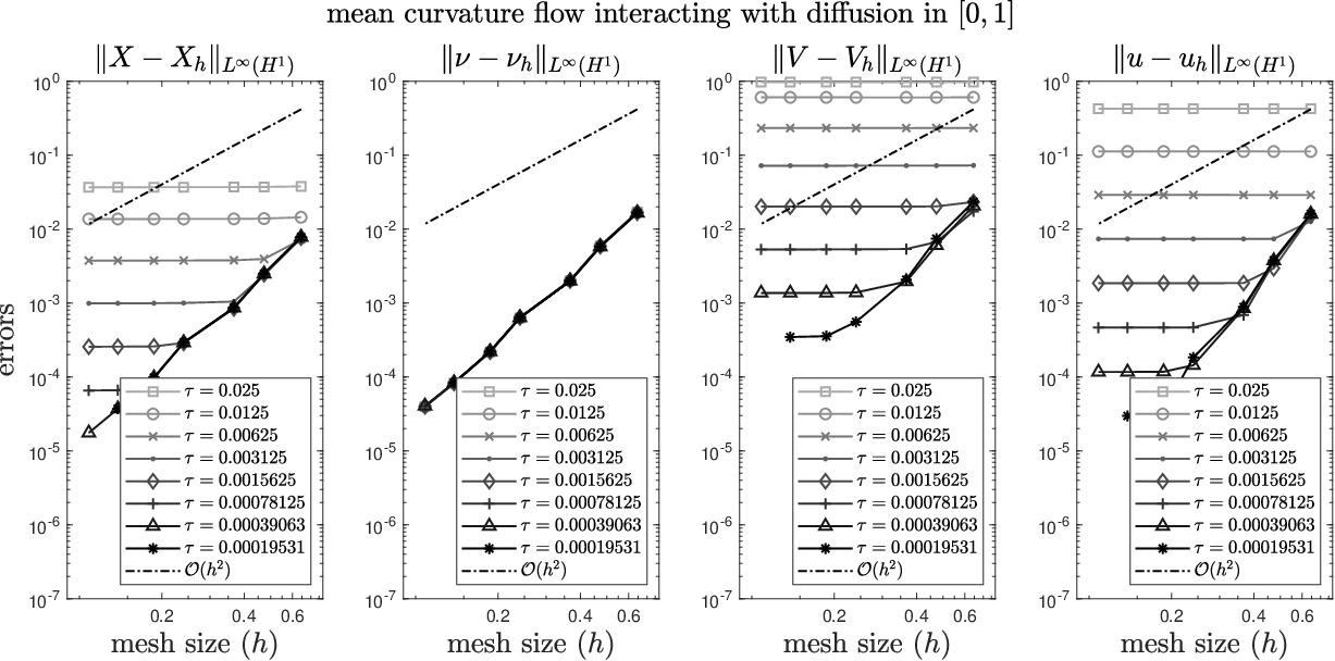
Refer to caption
Figure 2: Solutions (Γh​[𝐱]\Gamma_{h}[{\mathbf{x}}] and uhu_{h}) of the radially symmetric flow with α=2\alpha=2 computed using BDF2 / quadratic ESFEM (colorbar applies to all plots).
Refer to caption
Figure 3: Spatial convergence of the BDF2 / quadratic ESFEM discretisation for Problem 1 with T=1T=1 and α=2\alpha=2.
Refer to caption
Figure 4: Temporal convergence of the BDF2 / quadratic ESFEM discretisation for Problem 1 with T=1T=1 and α=2\alpha=2.

10.3 Convexity/non-convexity along the flow

It is well known that for mean curvature flow, Hui 84, a strictly convex surface shrink to a round point in finite time, and stays strictly convex throughout. For the flow (1) this is not true. In Figure 5 and 6, F⁡(u,H)=g⁡(u)​HF(u,H)=g(u)H and 𝒟⁡(u)≡1\mathcal{D}(u)\equiv 1 where g⁡(u)=G⁡(u)−G′​(u)​u=3​u−2g(u)=G(u)-G^{\prime}(u)u=3u^{-2}, which corresponds to the energy density G⁡(u)=u−2G(u)=u^{-2}. This problem satisfies our assumptions from Section 2. We respectively report on the evolution of an elongated ellipsoid as initial surface with an initial value u0u^{0} (concentrated along the tips with values≈5\text{values}\approx 5 decreasing in the middle to 0.50.5), and on the mass conservation, weak maximum principle, energy decay, and the mean convexity along the flow. The plots of Figure 5 show the flow until final time T=7.5T=7.5, where a pinch singularity occurs. The simulations used dof=4002\text{dof}=4002 for the number of degrees of freedom and a time step τ=0.01\tau=0.01, (the colorbar applies to all plots). We point out the crucial observation that the approaching singularity is detectable on the mass conservation plot. Note that in Remark 1 only the mass conservation of the spatial semi-discretisation was studied, but not that of the fully discrete numerical method (93). For Figure 6 (and the other experiments as well) the mass and energy were computed by quadratures.

Refer to caption
Figure 5: Unlike for mean curvature flow, convex surfaces do not remain convex along the flow (1) with F⁡(u,H)=g⁡(u)​H=3​u−2​HF(u,H)=g(u)H=3u^{-2}H (the colorbar applies to all plots).
Refer to caption
Figure 6: Mass conservation, weak maximum principle, energy decay, and mean convexity for the example in Figure 5 along the flow (1) with g⁡(u)=3​u−2g(u)=3u^{-2}.

10.4 Slow diffusion through a tight neck

The diffusion speed on surfaces is greatly influenced by the geometry, see, e.g., the insightful paper of Ecker Eck 08. To report on such an experiment for the flow (1a)–(1b), as an initial surface we take a dumbbell (given by (ES 12, equation (2.3))) and initial data u0u^{0} which is 0.80.8 from the neck above and smoothly transitioning to 10−410^{-4} for the neck and below. The experiment takes 𝒟⁡(u)≡1\mathcal{D}(u)\equiv 1 and F⁡(u,H)=u​HF(u,H)=uH. In view of these choices, and the initial data u0u^{0}, the bottom part barely moves, while the top part quickly shrinks before the concentration could pass through the neck. We note that for pure mean curvature flow of this initial surface a pinch-off singularity would occur in finite time, cf. (KLL 19, Figure 4) which uses the exact same initial surface Γ0\Gamma^{0}.

The experiment uses a mesh with dof=10522\text{dof}=10522 and a time step size τ=0.001\tau=0.001. In Figure 7 we observe that, since the diffusion speed at the neck is rather slow, the concentration uhu_{h} cannot equidistribute before the top part is vanishing. A pinch-off does not occur, contrary to standard mean curvature flow, see (KLL 19, Section 13.2) (using the same initial surface). Similarly as before, Figure 8 reports on the mass conservation, weak maximum principle, and the mean convexity along the flow, we note however that the initial surface is not mean convex: min{H(⋅,0)}≈−1.72⋅10−12\min\{H(\cdot,0)\}\approx-1.72\cdot 10^{-12}. Note the axis-limits in Figure 8.

Refer to caption
Figure 7: The diffusion speed is slow at a tight neck, and hence the large concentration differences cannot equilibrate before the top part shrinks along the flow (1) with F⁡(u,H)=u​HF(u,H)=uH and 𝒟⁡(u)≡1\mathcal{D}(u)\equiv 1.
Refer to caption
Figure 8: Mass conservation, weak maximum principle (note the axis-scaling), and mean convexity for the example in Figure 7, along the flow(1) with F⁡(u,H)=u​HF(u,H)=uH and 𝒟⁡(u)≡1\mathcal{D}(u)\equiv 1.

10.5 A self-intersecting flow

The flow (1) may describe surface evolutions where Γ⁡[X]\Gamma[X] is self intersecting, i.e. X⁡(⋅,t):Γ0→ℝ3X(\cdot,t)\colon\Gamma^{0}\rightarrow\mathbb{R}^{3} is not a parametrisation, but an immersion, see the similar construction in (Bür 21, Figures 5.3–5.5). We consider the flow (1) with F⁡(u,H)=g⁡(u)​HF(u,H)=g(u)H and 𝒟⁡(u)≡1\mathcal{D}(u)\equiv 1 where g⁡(u)=G⁡(u)−G′​(u)​u=5​u−4g(u)=G(u)-G^{\prime}(u)u=5u^{-4}, which corresponds to the energy density G⁡(u)=u−4G(u)=u^{-4}. This problem satisfies our assumptions from Section 2.

For a cup shaped surface11 1 Generated in Blender: blender.org. (with dof=4002\text{dof}=4002) and a suitably chosen initial value self-intersections are possible. The initial datum is chosen such that u0u^{0} is constant 10 over the whole surface Γ0\Gamma^{0}, except on the outer-bottom where it is gradually decreased to a smaller value≈1\text{value}\approx 1 as shown in the leftmost plot in Figure 10. In Figure 9 and 10 we present the numerical solution obtained by the 2-step BDF method with τ=10−3\tau=10^{-3}. The self-intersection is clearly observable on both figures, e.g., note the bright patch in Figure 10 after the self intersection. Of course the self-intersection does not influence the mass conservation, weak maximum principle, and energy decay, see Figure 11. (The initial surface is clearly not convex.)

Refer to caption
Figure 9: Snapshots (cross section at the x=0x=0 plane) of a self-intersecting evolution (1) with F⁡(u,H)=g⁡(u)​H=5​u−4​HF(u,H)=g(u)H=5u^{-4}H and 𝒟⁡(u)≡1\mathcal{D}(u)\equiv 1.
Refer to caption
Figure 10: Snapshots of the surface Γh​[𝐱]\Gamma_{h}[{\mathbf{x}}] and the concentration uhu_{h} (bottom view of the xx–yy-projection) of a self-intersecting evolution (1) with F⁡(u,H)=g⁡(u)​H=5​u−4​HF(u,H)=g(u)H=5u^{-4}H and 𝒟⁡(u)≡1\mathcal{D}(u)\equiv 1.
Refer to caption
Figure 11: Mass conservation, weak maximum principle and energy decay for the self-intersecting example in Figure 9–10 along the flow (1) with g⁡(u)=5​u−4g(u)=5u^{-4}.

Acknowledgments

We thank Stefan Schmidt for his Blender magic regarding the initial cup surface. The work of Harald Garcke and Balázs Kovács is supported by the DFG Graduiertenkolleg 2339 IntComSin – Project-ID 321821685. The work of Balázs Kovács is funded by the Heisenberg Programme of the Deutsche Forschungsgemeinschaft (DFG, German Research Foundation) – Project-ID 446431602.

References

  • ABG [22] H. Abels, F. Bürger, and H. Garcke. Qualitative properties for a system coupling scaled mean curvature flow and diffusion. arXiv:2205.02493, 2022.
  • ACYZ [21] G. Akrivis, M. Chen, F. Yu, and Z. Zhou. The energy technique for the six-step BDF method. SIAM J. Math. Anal., 59, 2021.
  • AES [15] A. Alphonse, C. M. Elliott, and B. Stinner. An abstract framework for parabolic PDEs on evolving spaces. Portugaliae Mathematica, 72(1):1–46, 2015.
  • AL [15] G. Akrivis and C. Lubich. Fully implicit, linearly implicit and implicit–explicit backward difference formulae for quasi-linear parabolic equations. Numer. Math., 131(4):713–735, 2015.
  • ALL [17] G. Akrivis, B. Li, and C. Lubich. Combining maximal regularity and energy estimates for time discretizations of quasilinear parabolic equations. Math. Comp., 86(306):1527–1552, 2017.
  • BCH [06] S. Bartels, C. Carstensen, and A. Hecht. P2Q2Iso2D=2​D\rm P2Q2Iso2D=2D isoparametric FEM in Matlab. J. Comput. Appl. Math., 192(2):219–250, 2006.
  • BDS [17] J. W. Barrett, K. Deckelnick, and V. Styles. Numerical analysis for a system coupling curve evolution to reaction diffusion on the curve. SIAM J. Numer. Anal., 55(2):1080–1100, 2017.
  • BEM [11] R. Barreira, C. M. Elliott, and A. Madzvamuse. The surface finite element method for pattern formation on evolving biological surfaces. J. Math. Biol., 63(6):1095–1119, 2011.
  • BGN [08] J. W. Barrett, H. Garcke, and R. Nürnberg. On the parametric finite element approximation of evolving hypersurfaces in ℝ3\mathbb{R}^{3}. J. Comput. Phys., 227(9):4281–4307, 2008.
  • BGN [20] J. W. Barrett, H. Garcke, and R. Nürnberg. Parametric finite element approximations of curvature driven interface evolutions. In Andrea Bonito and Ricardo H. Nochetto, editors, Handb. Numer. Anal., volume 21, pages 275–423. Elsevier, Amsterdam, 2020.
  • [11] T. Binz and B. Kovács. A convergent finite element algorithm for generalized mean curvature flows of closed surfaces. IMA J. Numer. Anal., 2021. doi:10.1093/imanum/drab043.
  • [12] T. Binz and B. Kovács. A convergent finite element algorithm for mean curvature flow in higher codimension. arXiv:2107.10577, 2021.
  • BS [08] S.C. Brenner and R. Scott. The mathematical theory of finite element methods, volume Texts in Applied Mathematics, 15. Springer, New York, 2008.
  • Bür [21] F. Bürger. Interaction of mean curvature flow and diffusion. PhD thesis, University of Regensburg, Regensburg, Germany, 2021. doi:10.5283/epub.51215.
  • CGG [01] M. A. J. Chaplain, M. Ganesh, and I. G. Graham. Spatio-temporal pattern formation on spherical surfaces: numerical simulation and application to solid tumour growth. J. Math. Biol., 42(5):387–423, 2001.
  • DDE [05] K. Deckelnick, G. Dziuk, and C. M. Elliott. Computation of geometric partial differential equations and mean curvature flow. Acta Numerica, 14:139–232, 2005.
  • DE [07] G. Dziuk and C. M. Elliott. Finite elements on evolving surfaces. IMA J. Numer. Anal., 27(2):262–292, 2007.
  • [18] G. Dziuk and C. M. Elliott. Finite element methods for surface PDEs. Acta Numerica, 22:289–396, 2013.
  • [19] G. Dziuk and C. M. Elliott. L2L^{2}–estimates for the evolving surface finite element method. Math. Comp., 82(281):1–24, 2013.
  • Dem [09] A. Demlow. Higher–order finite element methods and pointwise error estimates for elliptic problems on surfaces. SIAM J. Numer. Anal., 47(2):805–807, 2009.
  • DKM [13] G. Dziuk, D. Kröner, and T. Müller. Scalar conservation laws on moving hypersurfaces. Interfaces Free Bound., 15(2):203–236, 2013.
  • DLM [12] G. Dziuk, C. Lubich, and D. E. Mansour. Runge–Kutta time discretization of parabolic differential equations on evolving surfaces. IMA J. Numer. Anal., 32(2):394–416, 2012.
  • DS [22] K. Deckelnick and V. Styles. Finite element error analysis for a system coupling surface evolution to diffusion on the surface. Interfaces Free Bound., 24:63–93, 2022.
  • Dzi [88] G. Dziuk. Finite elements for the Beltrami operator on arbitrary surfaces. Partial differential equations and calculus of variations, Lecture Notes in Math., 1357, Springer, Berlin, pages 142–155, 1988.
  • Dzi [90] G. Dziuk. An algorithm for evolutionary surfaces. Numer. Math., 58(1):603–611, 1990.
  • Eck [04] K. Ecker. Regularity theory for mean curvature flow, volume 57 of Progress in Nonlinear Differential Equations and their Applications. Birkhäuser Boston, Boston, MA, 2004.
  • Eck [08] K. Ecker. Heat equations in geometry and topology. Jahresber. Deutsch. Math.-Verein., 110(3):117–141, 2008.
  • EF [17] C. M. Elliott and H. Fritz. On approximations of the curve shortening flow and of the mean curvature flow based on the DeTurck trick. IMA J. Numer. Anal., 37(2):543–603, 2017.
  • EKS [19] J. Eyles, J. R. King, and V. Styles. A tractable mathematical model for tissue growth. Interfaces Free Bound., 21(4):463–493, 2019.
  • ER [21] C. M. Elliott and T. Ranner. A unified theory for continuous-in-time evolving finite element space approximations to partial differential equations in evolving domains. IMA Journal of Numerical Analysis, 41:1696–1845, 2021.
  • ES [12] C. M. Elliott and V. Styles. An ALE ESFEM for solving PDEs on evolving surfaces. Milan Journal of Mathematics, 80(2):469–501, 2012.
  • HP [99] G. Huisken and A. Polden. Geometric evolution equations for hypersurfaces. In Calculus of variations and geometric evolution problems (Cetraro, 1996), volume 1713 of Lecture Notes in Math., pages 45–84. Springer, Berlin, 1999.
  • Hui [84] G. Huisken. Flow by mean curvature of convex surfaces into spheres. J. Differential Geometry, 20(1):237–266, 1984.
  • HW [96] E. Hairer and G. Wanner. Solving Ordinary Differential Equations II. Stiff and Differential–Algebraic Problems. Springer, Berlin, Second edition, 1996.
  • KL [21] B. Kovács and B. Li. Maximal regularity of backward difference time discretization for evolving surface PDEs and its application to nonlinear problems. arXiv:2106.07951, 2021.
  • KLL [19] B. Kovács, B. Li, and C. Lubich. A convergent evolving finite element algorithm for mean curvature flow of closed surfaces. Numer. Math., 143:797–853, 2019.
  • KLL [20] B. Kovács, B. Li, and C. Lubich. A convergent algorithm for forced mean curvature flow driven by diffusion on the surfaces. Interfaces Free Bound., 22(4):443–464, 2020.
  • KLL [21] B. Kovács, B. Li, and C. Lubich. A convergent evolving finite element algorithm for Willmore flow of closed surfaces. Numerische Mathematik, 149(4):595–643, 2021.
  • KLLP [17] B. Kovács, B. Li, C. Lubich, and C.A. Power Guerra. Convergence of finite elements on an evolving surface driven by diffusion on the surface. Numer. Math., 137(3):643–689, 2017.
  • Kov [18] B. Kovács. High-order evolving surface finite element method for parabolic problems on evolving surfaces. IMA J. Numer. Anal., 38(1):430–459, 2018.
  • KP [16] B. Kovács and C.A. Power Guerra. Error analysis for full discretizations of quasilinear parabolic problems on evolving surfaces. NMPDE, 32(4):1200–1231, 2016.
  • Li [21] B. Li. Convergence of Dziuk’s semidiscrete finite element method for mean curvature flow of closed surfaces with high-order finite elements. SIAM J. Numer. Anal., 59(3):1592–1617, 2021.
  • LMV [13] C. Lubich, D.E. Mansour, and C. Venkataraman. Backward difference time discretization of parabolic differential equations on evolving surfaces. IMA J. Numer. Anal., 33(4):1365–1385, 2013.
  • NO [81] O. Nevanlinna and F. Odeh. Multiplier techniques for linear multistep methods. Numerical Functional Analysis and Optimization, 3(4):377–423, 1981.
  • PS [04] P-O. Persson and G. Strang. A simple mesh generator in MATLAB. SIAM Review, 46(2):329–345, 2004.
  • PS [17] P. Pozzi and B. Stinner. Curve shortening flow coupled to lateral diffusion. Numer. Math., 135(4):1171–1205, 2017.
  • PS [19] P. Pozzi and B. Stinner. Elastic flow interacting with a lateral diffusion process: the one-dimensional graph case. IMA J. Numer. Anal., 39(1):201–234, 2019.
  • SVY [21] V. Styles and J. Van Yperen. Numerical analysis for a system coupling curve evolution attached orthogonally to a fixed boundary, to a reaction-diffusion equation on the curve. Num. Meth. PDE, 2021.
  • Wal [15] S. W. Walker. The shape of things: a practical guide to differential geometry and the shape derivative. SIAM, Philadelphia, 2015.