Weakly Supervised Indoor Localization via Manifold Matching
Abstract
Inferring the location of a mobile device in an indoor setting is an open problem of utmost significance. A leading approach that does not require the deployment of expensive infrastructure is fingerprinting, where a classifier is trained to predict the location of a device based on its captured signal. The main caveat of this approach is that acquiring a sufficiently large and accurate training set may be prohibitively expensive. Here, we propose a weakly supervised method that only requires the location of a small number of devices. The localization is done by matching a low-dimensional spectral representation of the signals to a given sketch of the indoor environment. We test our approach on simulated and real data and show that it yields an accuracy of a few meters, which is on par with fully supervised approaches. The simplicity of our method and its accuracy with minimal supervision makes it ideal for implementation in indoor localization systems.
1 Introduction
The development of algorithms for indoor positioning based on Wi-Fi or cellular signals has gained considerable interest in recent years due to their applicability to location-based services. These services include, for example, network management, security, healthcare, and emergency navigation as well as many commercial applications [37, 16]. A typical setting includes a small number of receivers that capture signals transmitted by multiple mobile devices whose location is unknown. The task is to infer the position of these mobile devices solely based on the captured signals.


In an outdoor setting, the problem is readily solved by using triangulation based on GPS signals. This approach is applicable since the transmitter (e.g., satellite ) has a direct Line-Of-Sight connection with the users (e.g., cellphones). In an indoor setting, however, the transmitted signal is usually reflected, scattered, shadowed, or diverted from the Line-Of-Sight [35]. The result of these diversions is the “multipath” phenomenon where the transmitted signal propagates through different paths to the receiver, see illustration in Figure 1. The problem of indoor localization thus requires a different approach. A hardware-oriented method to enable positioning involves distributing a large number of receivers throughout the indoor area. This will mitigate the “multipath” phenomenon and enable positioning through triangulation by the closest receivers. The caveat of this method is the high cost and complexity of deploying such a large network of receivers [22, 25].
An alternative, data-oriented approach that does not require expensive infrastructure is called fingerprinting. Here, the task of indoor positioning is cast as a supervised learning problem. First, a training set is obtained by capturing signals through the receivers while positioning a transmitter at multiple known locations. From each transmitted signal, we extract a fingerprint, a set of features of the signal that characterizes the transmitter’s location. Common features include, among others, the signal’s strength, [1] the channel information [36] and multi-path time and direction of arrival [34, 18, 15] . This dataset is used to train a classifier that predicts, for new captured signals, the location from which they were transmitted [8].
One major problem of the fingerprinting approach for applications requiring high accuracy is that recording and maintaining a suitable labeled data set may be prohibitively expensive. In contrast, collecting even vast amounts of unlabeled data may be done simply by recording the Wi-Fi signals of various devices moving through the venue. This fact motivates a “weakly supervised fingerprinting” problem, in which, except for a small number of points, the given data includes only the received signals without their transmitted locations. The objective is to estimate the location from which the signals were transmitted.
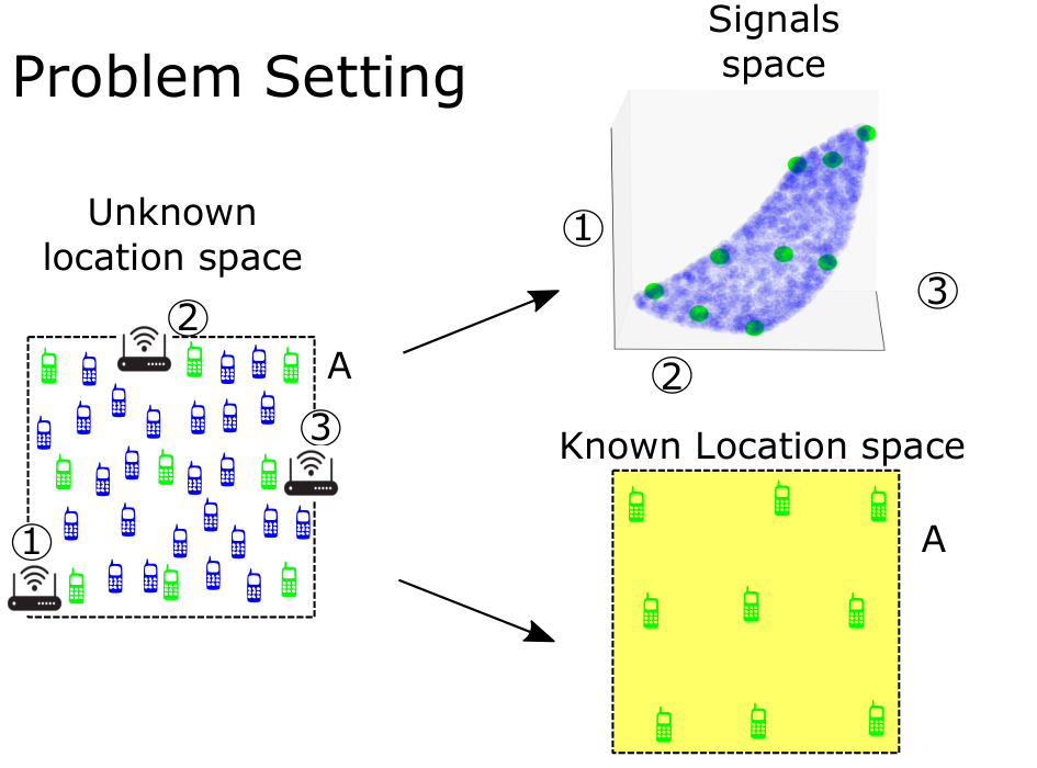
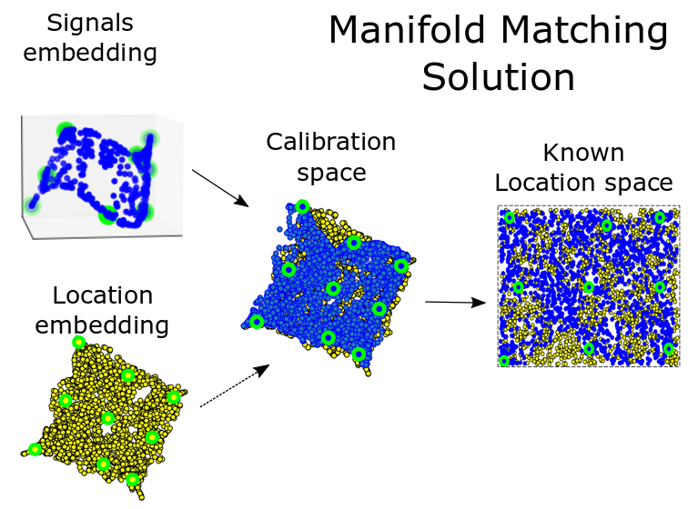
This work aims to tackle this semi-supervised problem while assuming that the shape of the indoor environment is provided. Our approach is based on matching a spectral representation of the captured signals to a spectral representation of the given indoor environment. To that end, we use a small number of signals whose location is known as calibration points that enable accurate matching between the two representations. The problem, along with our approach for its solution, is illustrated in Figure 2.
This paper proceeds as follows: In Section 2 we provide a line of relevant work and describe how our setting relates to other problems of semi-supervised learning. In Section 3 we formally define our framework and our model assumptions. The steps for our manifold-matching approach for indoor localization are outlined in Section 4. Experiments on simulated and real data are presented in Section 5. The paper concludes with Figure 7, where we discuss potential improvements and future work.
2 Related work
The weakly supervised Wifi localization problem that we tackle in this paper is, at its core, a semi-supervised problem. The task is to estimate the locations (labels) of a large set of unlabeled signals given a small subset of labeled ones. The classic semi-supervised setting is addressed in [4, 2, 5] where the goal is to compute a low-dimensional representation for the given data that is smooth with respect to a computed graph but also similar, for a subset of points, to their provided labels. Similar semi-supervised methods were used, among others, for image and text classification [39, 12], see extensive review in [40].
The main difference between our problem and the classic semi-supervised settings is that we are given, as side information, the shape of the area from which the points were transmitted. As we show, under appropriate assumptions, it is possible to leverage the geometric structure of the area to compute a correspondence between the signals and the location from which they were transmitted.
Challenges that include matching signals to a given shape exist in many other domains. In [33] the goal is to perform matrix completion by computing a map between two trajectories. Another example is the explainability of latent variables [17]. Here, the goal is to unveil connections between the graph’s eigenvectors and user-defined functions that originate from domain knowledge. In computer vision, a classic challenge is to computing a correspondence between and surfaces [27, 21].
For cases where additional local information is available (in the form of systematic small perturbations), anisotropic diffusion maps can be used to map the signal space to the floor plan geometry [30]. This matching can be accomplished via an orthogonal transformation between the two embeddings, needing very few known registration points. A neural network architecture implementing a similar procedure has been published in [26]. Here, the neural network find an embedding to the signal space that matches, up to orthogonal transformation, to the floor plan map.
For the application of indoor localization, a semi-supervised approach was derived in [24], where a signal’s location was estimated based on its geodesic distance to the closest signal whose location is known. In a recent paper, [13] derived an approach for indoor localization that is based on the given shape of the indoor environment. Their algorithm computes a map between the signals and their locations by optimal transport. This approach, however, requires a partial label in the form of a room or zone of the given signals. In contrast to [13] , our approach computes a transformation between a graph-based representation of the signals, and a graph-based representation of the reference floor plan. We show that a small number of signals with known locations suffice for computing this transformation and obtaining localization accuracy of a few meters.
3 Problem setting
We consider an array of receivers and transmission devices located in an area denoted by . For example, may be a single floor area in an office building, a mall, or an airport. Each device transmits a set of signals from approximately the same location, which are captured by the receivers. We denote the location of the th device by and the set of its transmitted signals by . We assume that the locations of a small number of devices are known, where . These can be, for example, the location of stationary transmitters that repeatedly communicate with the receivers. The locations of the rest of the devices are unknown, and our goal is to provide an accurate estimate of them. Figure 2 illustrates our setting.
Clearly, this task is not possible without additional assumptions. Here, we make the following assumptions on the input signals.
Assumption 3.1.
Uniform sampling- we denote by a random variable with a uniform distribution over . The locations are independent realizations of .
Assumption 3.2.
Sufficient Sampling - is sufficiently large to cover the entire area with high resolution.
Assumption 3.3.
Smoothness - the signal is a bilipschitz function of the location and a small set of parameters , that are independent of the locations. Example for such parameters include transmittor type, orientation etc. Thus, the signals forms a low dimensional manifold embedded in a -dimensional space.
The above assumptions are standard in the literature of indoor positioning [15, 13]. In Figure 7, we discuss the common case where a physical barrier in the indoor enviornment causes the signal to be discontinuous. In section 4 we leverage our knowledge of as well as the location of the transmitters to infer the location of the other devices.
| - Build a graph on the signals by applying on |
|---|
| - Compute the normalized Laplacian , as in Eq. (1) |
| - Generate an embedding as in Eq. (2) |
| - Sample uniformly from |
| - Build a graph on the sampled locations |
| using a normalized Gaussian kernel |
| - Compute the normalized Laplacian |
| - Generate an embedding , as in Eq. (2) |
4 Indoor localization via manifold matching
In this section we derive the steps of our localization approach in detail.
A tale of two graphs.
Constructing a neighborhood graph is a common approach in manifold learning. Here, we compute two such graphs. The nodes of the signal graph, denoted by , correspond to the transmitting devices. The weight between a pair of nodes is calculated based on a predefined local kernel function . The choice of depends on the characteristics of the captured signals. Importantly, the smoothness assumption implies that pairs of nodes connected by an edge with a large weight correspond to devices located at close locations within .
The second graph, denoted is the area graph, which is computed based on our knowledge of the shape of . First, we generate a set of points, denoted by sampled uniformly over . We assume that the first points are identical to the ones of the previous graph, such that . Each node corresponds to one random location . The weight between two nodes is computed by a normalized Gaussian kernel with as input.
For both graphs, we compute a symmetric normalized Laplacian matrix, given by
| (1) | |||
where and are diagonal matrices with elements and , respectively. Following [3, 9]. Let be, respectively, the eigenvectors of and that correspond to the -th smallest eigenvalues. We compute a new representation for the nodes in both graphs using the eigenvectors of the respective Laplacian matrix by
| (2) | |||
Our approach builds upon the relation between the two graphs and and their representation based on their spectrum. As shown in [14, 29, 32, 3, 11], given a sufficiently large number of samples and signals from the area , the eigenvectors and converge to the eigenfunctions of the Laplace-Beltrami operator on their respective manifolds. These eigenfunctions capture important geometric information of the underlying manifold, see [3, 9].
3.3 implies that the signals are fully determined by their location . However, the eigenvectors of the signal graph can be very different from the corresponding eigenvectors of the area graph . Let us give a concrete example. Assume that . For the graphs and we sampled a set of and points uniformly at random over the area . The high dimensional signals are given by
| (3) |
where is a random matrix and is some point outside . The term can be understood as the result of a power decay due to the distance to a receiver. This factor implies that points with a similar distance to will be more strongly connected than points at different distances, which distorts the original manifold structure.

The left column of Figure 3 shows the two leading eigenvectors of the area graph . Since is a square, each of the two leading eigenvectors is a cosine function of one of its coordinates. The middle column shows the two leading eigenvectors of . It is evident that these vectors depend mainly on the radial effect caused by the non linear function . Thus, the challenge is to calibrate these eigenvectors and extract the information relevant for localization from the signal’s graph. The process computing a calibration matrix is described in the following section.
Matching spectral representation.
Our goal is to extract from the signal embedding a calibrated representation that is consistent with the area , and thus useful for localization. We denote the calibrated representation function by . On the one hand, should preserve the geometry of the signals, and thus be smooth with respect to the signal graph . On the other hand, for the points whose location is known, we would like the calibrated representation to be similar to the corresponding representation of the locations . This motivates the following optimization problem:


The right term in Eq. (4) is a regularization term, which gives a penalty for using high-frequency eigenvectors from the spectrum of . Similar regularization terms appear in several problems that include graph based regularizations, see for example [2, 12, 20]. In a typical setting, the solution of Eq. (4) is a linear function of a maximum of eigenvectors with the smallest eigenvalues of . To improve robustness, we limit the new representation to be a linear combination of the eigenvectors with the smallest eigenvalues,
| (4) |
where is the calibration matrix. We slightly abuse notation by denoting the signals embedding matrix by . Inserting Eq. (4) to Eq. (4) yields a quadratic optimization problem with the following closed form solution,
The right column in Figure 3 shows the first two calibrated signal vectors for the artificial signal given in Eq. (3). The number of shared points is , and the dimensions of the signals’ and locations’ representation is equal to and , respectively. Though the calibration is done by a relatively small number of points, the new vectors indeed extract the information on the coordinates while leaving out other dependencies, such as the radial term. Our final step is to use the calibrated vectors in order to obtain an accurate localization for all signals.
Remark 4.1.
For the vectors , we select the eigenvectors with the smallest eigenvalue of the Laplacian matrix. These are the smoothest orthogonal vectors with respect to the area graph. A possible alternative for is to compute the leading independent harmonics of . These consist of a subset of eigenvectors that are non-redundant, in the sense that each captures a different coordinate in the original manifold, see [7, 10]. A simple example where such an approach may be beneficial is a long rectangular area, where the eigenvectors with the smallest eigenvalues will all encode the same coordinate. In such a case, taking independent harmonics may guarantee that we obtain non-redundant eigenvectors, that are sufficient for localization.
Localization via 1-nearest neighbor
Finally, based on the calibrated coordinates, we estimate the location of any unknown point by a simple -nn search,
| (5) |
In other words, we search for the point that after calibration, has the closest representation to . Algorithm 1 summarizes the different steps of our localization pipeline.
5 Experimental results
We validate our localization approach on simulated and real datasets captured in an office environment. In the first experiment, we use the simulated dataset generated in [18] by a 3D wave propagation software. The floor plan of this simulation is shown in Figure 1. In our second experiment, we test our approach on a real Wifi signal dataset generated in [31]. The code for reproducing our results is provided as supplementary material.
5.1 Simulated Wifi experiment
In our first experiment, the area is a rectangular office environment of size illustrated in Figure 1. The dataset consists of signals of dimension along with their transmitted locations. The subsets of signals and the local metric function are defined similarly to [18, 15, 24]. Specifically, we subsampled random locations from the dataset (). For each subsampled point , we defined a signal set as the concatenation of the signals with the closest transmitted location to , within of the transmitted location. For the construction of the signal graph we follow the similarity criteria between subsets of signals derived in [18], see more details in Appendix B.
To construct , we sampled points over . The embedding dimensions are set to for the area graph and for the signal graph. The right panel in Figure 4 shows the two leading eigenfunctions of in yellow, and the calibrated eigenfunctions in blue. The figure shows that the calibration process matches the signal eigenfuncions to the area eigenfunctions.
The left two panels in Figure 4 show the localization error of our algorithm as a function of the number of shared points. As baseline, we compared the performance to a nn classifier that assigns each signal to the closest labeled point. Our semi-supervised approach shows a clear advantage. For the median error of our estimate is equal to m and the mean error is . For additional comparison, in [24] the same dataset was tested, and a mean error of was achieved with labeled points. We thus reach a similar accuracy with around of the labeled points.
5.2 Wifi received signal strength experiment
The second experiment is based on a Wifi signal dataset generated in [31]. The dataset consists of the received signal strength measured by receivers, in an area of floors of buildings ( floors each). At each point , messages were transmitted and captured. Let denote a matrix whose elements contain the signal strength of messages transmitted from locations . For the signal graph we computed the median signal , equal to
The left panel in Figure 5 shows the values of for different locations . For this floor, only out of receivers captured one of the message.
For the graph the weight matrix is computed by a normalized Gaussian kernel . For the graph , we sampled points in the area of the transmitted signals. The middle panel of Figure 5 shows, as background, one of the floors from which signals were sent. The left column shows the simulated points, colored by their values in two eigenvectors of . Similarly, the middle column shows the locations of the actual signals, colored by their values in two eigenvectors of . The right column shows the calibrated vectors with calibration points. The location of the shared points was chosen by running k-means on the signal dataset. Figure 6 shows the median error as a function of the number of shared points for three different floors. Similarly to the first experiment, we compare our performance to a nn classifier. The results show a clear advantage and demonstrate the importance of learning the intrinsic structure of the signals for localization.


6 Discussion


Choice of parameters.
Algorithm 1 accepts, as input, three parameters whose choice may impact its accuracy: the dimensions , of the signal and area embeddings, and the regularization parameters . One simple approach for selecting these parameters is using the shared points for cross validation by computing the calibrated vectors and testing the performance on non-overlapping subsets of the shared points.
Applying cross-validation may be problematic, however, when the number of points is small. Inspired by the Iterative Closest Point algorithm [6], we propose an alternative approach that measures how well the area manifold and the signal manifold match after calibration, see for example Figure 4. For determining we define the following loss function:
| (6) |
We propose to determine by minimizing the loss in Eq. (6). We tested this approach for one of the datasets in [31], which was used for our Wifi experiment. The left panel in Figure 8 (Appendix) shows the performance of our Manifold Matching approach as a function of . The right panel shows the value of as defined in Eq. (6). The two curves are highly correlated, and achieve a minima around . This suggests that the matching based loss function is a valid way to choose for cases where the number of shared points is small. This approach may be used to select the embedding dimension as well. The choice of by this approach is more problematic as the loss increases with the dimension .


Integrating additional signals.
Once a match has been found between the signal space and the location space, the location of a new signal can be obtained by finding the signal with the most similar features. Let be the estimated location of , then
Other techniques can be employed for the out-of-sample-extension, an example for such is the Nystorm extension to infer the new signal embedding based on the known signals as discussed in [19]. In some cases, one would like to integrate incoming signals so as to improve the quality of the original data. To that end, recent works implemented neural network architectures to compute spectral embeddings of new data points [23, 28].
Discontinuity.
The indoor multipath phenomena, in which a signal propagates along different trajectories, poses multiple problems for indoor localization. One such problem is that the features of a received signal transmitted from two sides of a concrete wall may be very different. Disregarding such effects may harm the performance of our approach as the smoothness assumption (3.3) is strongly violated. To illustrate the effect of a physical barrier, we repeated the experiment described in section 4, but with a slight modification. We assume that there is a vertical wall that causes a diffraction pattern, see Figure 7. To model diffraction, we replace the Euclidean distance in Eq. (3) with a geodesic distance, denoted by . Specifically, the signal space is computed based on the following transformation,
| (7) |
Assuming the location of the barrier is known, it can be taken into account when computing the area graph . This can be done by using the geodesic distance for the area graph . This will effectively remove connections between points at two sides of a wall. The right panels of Figure 7 show the spectral embedding of of (left column), the signal embedding (middle column) and the calibrated signal (right column). Taking into account the barrier simplifies the calibration process as the discontinuity appears both in the eigenvecors of and those of .
Independent harmonics.
In remark 4.1, we mentioned the possibility of using the leading independent harmonics instead of the eigenvectors with the smallest eigenvalue. This may insure that we gain sufficient information for each coordinate of the area . A related question for future research is the number of eigenvectors or independent harmonics one requires to obtain accurate localization. On the one hand, a single eigenvector for each coordinate may simplify calibration and thus the required number of shared points. On the other hand, a localization process based on a single eigenvector for each coordinate may be sensitive to noise. For example, the first harmonic of a rectangular area is a cosine function with low frequency, which has a very low gradient in areas close to the borders of . Thus, even a small perturbation can cause a large localization error. Taking additional harmonics where the gradient is higher may thus is expected to increase the accuracy in these areas.
7 Acknowledgment
EP and IGK were partially supported by DARPA (ATLAS program, Dr. J. Zhou) and the US AFPSR (Dr. Fariba Fahroo). EP was partially supported by the Center for Interdisciplinary Data Science Research at the Hebrew University (CIDR). We would like to thank Mati Wax, Boris Landa and Ronald Coifman for for useful and insightful discussions.
References
- [1] Paolo Barsocchi, Stefano Lenzi, Stefano Chessa and Gaetano Giunta “A novel approach to indoor RSSI localization by automatic calibration of the wireless propagation model” In VTC Spring 2009-IEEE 69th Vehicular Technology Conference, 2009, pp. 1–5 IEEE
- [2] Mikhail Belkin, Irina Matveeva and Partha Niyogi “Regularization and semi-supervised learning on large graphs” In International Conference on Computational Learning Theory, 2004, pp. 624–638 Springer
- [3] Mikhail Belkin and Partha Niyogi “Laplacian eigenmaps for dimensionality reduction and data representation” In Neural computation 15.6 MIT Press, 2003, pp. 1373–1396
- [4] Mikhail Belkin and Partha Niyogi “Semi-supervised learning on Riemannian manifolds” In Machine learning 56.1 Springer, 2004, pp. 209–239
- [5] Mikhail Belkin, Partha Niyogi and Vikas Sindhwani “Manifold regularization: A geometric framework for learning from labeled and unlabeled examples.” In Journal of machine learning research 7.11, 2006
- [6] Paul Besl and Neil McKay “Method for registration of 3-D shapes” In Sensor fusion IV: control paradigms and data structures 1611, 1992, pp. 586–606 International Society for OpticsPhotonics
- [7] Yochai Blau and Tomer Michaeli “Non-redundant spectral dimensionality reduction” In Joint European Conference on Machine Learning and Knowledge Discovery in Databases, 2017, pp. 256–271 Springer
- [8] Hao Chen et al. “ConFi: Convolutional neural networks based indoor Wi-Fi localization using channel state information” In IEEE Access 5 IEEE, 2017, pp. 18066–18074
- [9] Ronald Coifman and Stéphane Lafon “Diffusion maps” In Applied and computational harmonic analysis 21.1 Elsevier, 2006, pp. 5–30
- [10] Carmeline Dsilva, Ronen Talmon, Ronald Coifman and Ioannis Kevrekidis “Parsimonious representation of nonlinear dynamical systems through manifold learning: A chemotaxis case study” In Applied and Computational Harmonic Analysis 44.3 Elsevier, 2018, pp. 759–773
- [11] David Dunson, Hau-Tieng Wu and Nan Wu “Spectral convergence of graph Laplacian and Heat kernel reconstruction in L infinity from random samples” In Applied and Computational Harmonic Analysis Elsevier, 2021
- [12] Rob Fergus, Yair Weiss and Antonio Torralba “Semi-Supervised Learning in Gigantic Image Collections.” In NIPS 1, 2009, pp. 2 Citeseer
- [13] Farhad Ghazvinian et al. “Modality-Agnostic Topology Aware Localization” In Advances in Neural Information Processing Systems 34, 2021
- [14] Matthias Hein, Jean-Yves Audibert and Ulrike Luxburg “Graph laplacians and their convergence on random neighborhood graphs.” In Journal of Machine Learning Research 8.6, 2007
- [15] Ariel Jaffe and Mati Wax “Single-site localization via maximum discrimination multipath fingerprinting” In IEEE Transactions on Signal Processing 62.7 IEEE, 2014, pp. 1718–1728
- [16] Ali Khalajmehrabadi, Nikolaos Gatsis and David Akopian “Modern WLAN fingerprinting indoor positioning methods and deployment challenges” In IEEE Communications Surveys & Tutorials 19.3 IEEE, 2017, pp. 1974–2002
- [17] Samson Koelle, Hanyu Zhang, Marina Meila and Yu-Chia Chen “Manifold coordinates with physical meaning” In arXiv e-prints, 2018, pp. arXiv–1811
- [18] Evgeny Kupershtein, Mati Wax and Israel Cohen “Single-site emitter localization via multipath fingerprinting” In IEEE Transactions on signal processing 61.1 IEEE, 2012, pp. 10–21
- [19] Stephane Lafon, Yosi Keller and Ronald Coifman “Data fusion and multicue data matching by diffusion maps” In IEEE Transactions on pattern analysis and machine intelligence 28.11 IEEE, 2006, pp. 1784–1797
- [20] Yuan Li et al. “Graph-Based Regularization for Regression Problems with Alignment and Highly Correlated Designs” In SIAM journal on mathematics of data science 2.2 SIAM, 2020, pp. 480–504
- [21] Or Litany, Emanuele Rodol‘a, Alexander Bronstein and Michael Bronstein “Fully spectral partial shape matching” In Computer Graphics Forum 36.2, 2017, pp. 247–258 Wiley Online Library
- [22] Junjie Liu and R Jain “Survey of wireless based indoor localization technologies” In Department of Science & Engineering, Washington University, 2014
- [23] Gal Mishne, Uri Shaham, Alexander Cloninger and Israel Cohen “Diffusion nets” In Applied and Computational Harmonic Analysis 47.2 Elsevier, 2019, pp. 259–285
- [24] Amit Moscovich, Ariel Jaffe and Nadler Boaz “Minimax-optimal semi-supervised regression on unknown manifolds” In Artificial Intelligence and Statistics, 2017, pp. 933–942 PMLR
- [25] Lionel Ni, Yunhao Liu, Yiu Lau and Abhishek Patil “LANDMARC: Indoor location sensing using active RFID” In Proceedings of the First IEEE International Conference on Pervasive Computing and Communications, 2003.(PerCom 2003)., 2003, pp. 407–415 IEEE
- [26] Erez Peterfreund et al. “Local conformal autoencoder for standardized data coordinates” In Proceedings of the National Academy of Sciences 117.49 National Acad Sciences, 2020, pp. 30918–30927
- [27] Emanuele Rodol‘a et al. “Partial functional correspondence” In Computer Graphics Forum 36.1, 2017, pp. 222–236 Wiley Online Library
- [28] Uri Shaham et al. “SpectralNet: Spectral Clustering using Deep Neural Networks” In International Conference on Learning Representations, 2018
- [29] Amit Singer “From graph to manifold Laplacian: The convergence rate” In Applied and Computational Harmonic Analysis 21.1 Elsevier, 2006, pp. 128–134
- [30] Amit Singer and Ronald Coifman “Non-linear independent component analysis with diffusion maps” In Applied and Computational Harmonic Analysis 25.2 Elsevier, 2008, pp. 226–239
- [31] Joaqu’in Torres-Sospedra et al. “UJIIndoorLoc: A new multi-building and multi-floor database for WLAN fingerprint-based indoor localization problems” In 2014 international conference on indoor positioning and indoor navigation (IPIN), 2014, pp. 261–270 IEEE
- [32] Nicol‘as‘a Trillos, Moritz Gerlach, Matthias Hein and Dejan Slepcev “Error estimates for spectral convergence of the graph Laplacian on random geometric graphs toward the Laplace–Beltrami operator” In Foundations of Computational Mathematics 20.4 Springer, 2020, pp. 827–887
- [33] Paul Villoutreix et al. “Synthesizing developmental trajectories” In PLoS computational biology 13.9 Public Library of Science San Francisco, CA USA, 2017, pp. e1005742
- [34] Yue Wang and KC Ho “TDOA positioning irrespective of source range” In IEEE Transactions on Signal Processing 65.6 IEEE, 2016, pp. 1447–1460
- [35] Klaus Witrisal and Paul Meissner “Performance bounds for multipath-assisted indoor navigation and tracking (MINT)” In 2012 IEEE International Conference on Communications (ICC), 2012, pp. 4321–4325 IEEE
- [36] Zheng Yang, Zimu Zhou and Yunhao Liu “From RSSI to CSI: Indoor localization via channel response” In ACM Computing Surveys (CSUR) 46.2 ACM New York, NY, USA, 2013, pp. 1–32
- [37] Faheem Zafari, Athanasios Gkelias and Kin Leung “A survey of indoor localization systems and technologies” In IEEE Communications Surveys & Tutorials 21.3 IEEE, 2019, pp. 2568–2599
- [38] Lihi Zelnik-manor and Pietro Perona “Self-Tuning Spectral Clustering” In Advances in Neural Information Processing Systems 17 MIT Press, 2005
- [39] Dengyong Zhou et al. “Learning with local and global consistency” In Advances in neural information processing systems, 2004, pp. 321–328
- [40] Xueyuan Zhou and Mikhail Belkin “Semi-supervised learning” In Academic Press Library in Signal Processing 1 Elsevier, 2014, pp. 1239–1269
Appendix A Computing the Kernel matrix
The normalized Gaussian kernel used in this paper is equal to
In all graphs, except the signal graph in experiment 1 and the discontinuity experiment in Section 7 the bandwidth was computed by
| (8) |
where returns the k-nearest neighbor index of . In the experiment discussed in the discontinuity paragraph in Figure 7, we use a self tuning kernel bandwidth as suggest in [38] where
Details for the signal graph of experiment 1 are given in Section 5.1.
Appendix B Computing the signal graph in experiment 1
Following [18, 24], we define for each point a second moment matrix , and a corresponding projection matrix given by
where is the -th leading eigenvector of . The similarities between to are determined by
| (9) |
where is the conjugate transpose operator. In [18], the location of an unknown point was estimated by the closest labeled point via Eq. (9). Here, we use Eq. (9) to obtain the graph . Specifically, the weight matrix of is set to be a binary nearest neighbor matrix based on defined by- if either or is among the most similar signals according to the other signal’s similarity criterion.
Appendix C Building 2 in Wifi experiment

