T-NGA: Temporal Network Grafting Algorithm for Learning to Process Spiking Audio Sensor Events

Fig. 1 illustrates the working principle of T-NGA. An RNN $\mathcal{F}(\cdot)$ is pretrained on spectrogram features extracted from the audio waveform samples. The pretrained network $\mathcal{F}(\cdot)$ consists of two parts: a front end $\mathcal{F}_{\text{front}}$ and trunk layers $\mathcal{F}_{\text{trunk}}$ (Fig. 1 (A)). The weights of the pretrained network are frozen during the T-NGA training. After training, a newly-trained grafted front end $\mathcal{G}_{\text{front}}(\cdot)$ together with the pretrained trunk layers $\mathcal{F}_{\text{trunk}}$ form a grafted network (GN) that processes event features computed from the spiking cochlea events (Fig. 1 (B)).

Let $\{(\mathbf{a}_{i},t_{i}^{a})\}_{i=1}^{T^{a}}$ and $\{(\mathbf{s}_{t},t_{i}^{s})\}_{i=1}^{T^{s}}$ be the temporally aligned spectrogram and event features where $t_{i}^{a}$ and $t_{i}^{s}$ are timestamps of $\mathbf{a}_{i}$ and $\mathbf{s}_{i}$ respectively. Note that $T^{a}$ may not be equal to $T^{s}$ depending on the choice of feature configuration (see Section 2.3).

$\mathcal{F}(\cdot)$ processes the spectrogram features $\{(\mathbf{a}_{i},t_{i}^{a})\}_{i=1}^{T^{a}}$ and returns the prediction $\{y_{l}\}_{l=1}^{L^{a}}$:

where $\{(\mathbf{h}_{i},t_{i}^{a})\}_{i=1}^{T^{a}}$ are the pretrained states, i.e., hidden states of $\mathcal{F}_{\text{front}}$. Similarly, GN processes event features $\{(\mathbf{s}_{t},t_{i}^{s})\}_{i=1}^{T^{s}}$ and outputs prediction $\{y_{l}^{s}\}_{l=1}^{L^{s}}$:

where $\{(\mathbf{g}_{i},t_{i}^{s})\}_{i=1}^{T^{s}}$ are the grafted states, i.e., hidden states of $\mathcal{G}_{\text{front}}$. The dimension of $\mathbf{g}_{i}$ is the same as the dimension of $\mathbf{h}_{i}$.

T-NGA training maximizes the similarity between $\{\mathbf{h}_{i}\}$ and $\{\mathbf{g}_{i}\}$. When $T^{a}\neq T^{s}$, we select $T$ features from both $\{\mathbf{h}_{i}\}$ and $\{\mathbf{g}_{i}\}$ where $T\leq\min(T^{a},T^{s})$ and timestamps of the corresponding states $t_{i}^{a}$ and $t_{i}^{s}$ are the closest in time. T-NGA training optimizes the following loss function:

where $\text{NCS}(\cdot,\cdot)$ and $\text{MAE}(\cdot,\cdot)$ compute the negative cosine similarity and the mean absolute error between aligned states, respectively. When the training is completed, the grafted front end $\mathcal{G}_{\text{front}}$ encodes the event features into a set of grafted states that can be directly used by the pretrained trunk layers $\mathcal{F}_{\text{trunk}}$.

The Dynamic Audio Sensor (DAS) has two independent 64-stage cascaded filter banks driven by two microphone inputs. The frequency selectivity of the cochlea channels ranges roughly from 50 Hz to 20 kHz on a log spacing across the channels. The DAS has been captured in several cochlea designs [5, 4, 15]. The spiking cochlea designed in [15] was used to generate the spike recordings of the TIDIGITS dataset to create a spiking cochlea dataset called N-TIDIGITS18. Details of this spiking dataset are given in Sec 2.5.

In this work, we also use a software model of a frequency channel which includes a second-order filter, a half-wave rectifier, and a linear leak integrate-and-fire neuron model used in the design reported in [15]. The transfer function of the $n$-th filter in a cascaded set of second-order filters is given by

where $\tau_{i}=\frac{1}{2\cdot\pi\cdot f_{i}}$, $f_{i}$ is the center frequency of the $i$-th channel, and $Q$ is the filter quality factor. The half-wave rectification is described as:

where $v_{r}$ is the rectifier output used to drive the neuron, $V_{n}$ is the filter output of the channel and $V_{\text{ref}}$ is a constant. The parameters of the model are set so that the spike responses of the channels are similar to those of the hardware spiking cochlea.

An example of the spikes generated from the software spiking cochlea model and the spikes recorded with the hardware spiking cochlea in response to the sample “8z1” (8Z1A.WAV from speaker AE in TIDIGITS) is shown in Fig. 2.

Features are extracted from both the audio and spike samples. For audio samples, we computed the Log-Mel spectrogram features using a 25 ms window, 10 ms stride, and 40 filter bank channels as shown in Fig. 3 (A). For the spike recordings, we used the time-binned spike count (TBSC) method [14] to convert spikes into event features. Assume that the spike stream consists of $N$ spikes $\{e_{i}=(t_{i},f_{i})\}_{i=1}^{N}$ where timestamps $t_{i}$ are in ascending order. The TBSC feature for a time window $\Delta W$ is then defined as $\mathbf{s}_{j}^{(f)}=\text{card}(\{e_{i}|t_{i}\in j\text{-th window},f_{i}=f\})$ where $\mathbf{s}_{j}^{(f)}$ represents TBSC feature value at $j$-th window for channel frequency $f$; $\text{card}(\cdot)$ is the cardinality of selected events. $\Delta W$ is 10 ms or 25 ms and the stride is 10 ms for the TBSC features used in the study. Examples of TBSC features with $\Delta W$= 25 ms are shown in Fig. 3 (B) and (C). For convenience, feature configurations are coded as window/stride, e.g., 25w/10s means 25 ms window and 10 ms stride.

The RNN used in this work consists of two Gated Recurrent Unit (GRU) [16] layers with 256 units each followed by a fully connected layer of 200 units with a LeakyReLU activation [17], and a final classification layer of 12 output units. The network has a total of 677 K parameters.

We used the men and women speaker recordings in the TIDIGITS dataset [18] to match the spike recordings in the N-TIDIGITS18 dataset [14]. N-TIDIGITS18 consists of 8,623 training samples and 8,700 testing samples. Each sample consists of a single digit or multiple spoken digits. In total, there are 11 digits (“o”, “zero” and “1” to “9”).

For T-NGA training, the N-TIDIGITS18 recordings and the corresponding audio samples were aligned temporally using the Dynamic Time Warping (DTW) algorithm [19] before feature extraction. The spike recordings generated by the software spiking cochlea model are already aligned with the corresponding audio samples.

We first trained a network PT-25 on TIDIGITS using spectrogram features as shown in Table 1(A). The PT-25 model was subsequently used as the pretrained model for T-NGA training to obtain grafted networks (GNs). For comparison, we also trained supervised networks (SNs) through standard supervised training on spiking cochlea datasets using event features.

Table 1(B) shows the results of using the event features created from ideal software spiking cochlea recordings. The GNs BGN-25, BGN-10 reached similar or better WERs than the SNs B-25, B-10. These result show that T-NGA training could be advantageous as it does not require a labeled event dataset and still produces a network that shows equivalent accuracy.

Results on N-TIDIGITS18 presented in Table 1(C) show that the SNs S-25, S-10 achieved $\sim$10% WER while the GNs GN-25, GN-10 reached $\sim$15% WER. The higher WER of the GNs compared to the corresponding SNs is because the hardware spiking cochlea includes circuit non-idealites that affect the distribution of the output cochlea spikes, and the temporal mismatch between the audio samples and event sample still exists after DTW alignment. In Section 3.2, we show that the WER of GN increased when training on spike recordings generated by the same software cochlea model which includes circuit non-idealities.

Table 1 also shows that both GNs and SNs perform better when using a 10w/10s event feature configuration, i.e., 10w/10s characterizes the spike recordings better than 25w/10s. T-NGA training for BGN-10 and GN-10 models used 25w/10s Log-Mel spectrogram features and 10w/10s TBSC features. The results show that T-NGA can maximize the similarity between temporally aligned grafted states and pretrained states successfully while the feature configurations for the two modalities are different.

We present two additional experiments to better understand the results obtained from T-NGA training and the resulting GN.

We first investigated quantitatively whether the circuit non-idealities of a spiking cochlea affect the performance of GN and SN. We generated another event dataset using the same software spiking cochlea model that includes circuit non-idealities from the the neuron spiking threshold, and filter quality factor variation. As a result, the WER of the GN was $\sim$3% higher than the SN as shown in Table 2. This result reveals that these non-idealities in the hardware spiking cochlea contributed to the gap in WER between GNs and SNs as observed in Table 1(C).

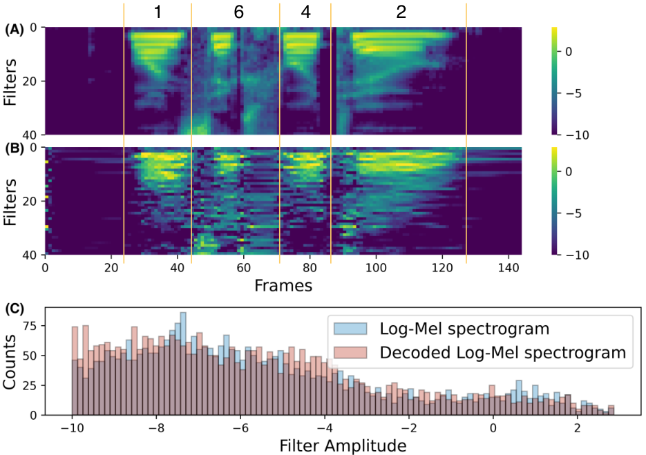
We also explored the encoded content in the grafted states of GN by decoding a given set of grafted states through the pretrained front end by following [13]. The outcome of this decoding procedure is a decoded Log-Mel spectrogram that represents the given grafted states. The optimization of this decoding procedure was carried out for 5,000 iterations using the Adam optimizer and a learning rate of 1e-2. To suppress the noise in the decoded Log-Mel spectrogram, we clipped the amplitude at -10. Fig. 4 shows a Log-Mel spectrogram that was decoded from the grafted states that were trained on a N-TIDIGITS18 sample. We found that the trained GN front end can generate the grafted features which often correctly represents the input audio signal. The decoded spectrogram shown in Fig. 4 (B) is visually similar to the original Log-Mel spectrogram shown in Fig. 4 (A). Fig. 4 (C) illustrates that the distributions of the amplitudes for the original and decoded spectrograms match well.

References

- [1] R. Prabhavalkar, R. Alvarez, C. Parada, P. Nakkiran, and T. N. Sainath, “Automatic gain control and multi-style training for robust small-footprint keyword spotting with deep neural networks,” in 2015 IEEE International Conference on Acoustics, Speech and Signal Processing (ICASSP), 2015, pp. 4704–4708.
- [2] C. Gao, S. Braun, I. Kiselev, J. Anumula, T. Delbruck, and S. Liu, “Real-time speech recognition for IoT purpose using a delta recurrent neural network accelerator,” in 2019 IEEE International Symposium on Circuits and Systems (ISCAS), May 2019, pp. 1–5.
- [3] B. Zhang, W. Li, Q. Li, W. Zhuang, X. Chu, and Y. Wang, “Autokws: Keyword spotting with differentiable architecture search,” in 2021 IEEE International Conference on Acoustics, Speech and Signal Processing (ICASSP), 2021, pp. 2830–2834.
- [4] S.-C. Liu, A. van Schaik, B. A. Minch, and T. Delbruck, “Asynchronous binaural spatial audition sensor with 2644 channel output,” IEEE Transactions on Biomedical Circuits and Systems, vol. 8, no. 4, pp. 453–464, 2014.
- [5] M. Yang, C.-H. Chien, T. Delbruck, and S.-C. Liu, “A 0.5 V 55 64 2 channel binaural silicon cochlea for event-driven stereo-audio sensing,” IEEE Journal of Solid-State Circuits, vol. 51, no. 11, pp. 2554–2569, 2016.
- [6] J. Anumula, E. Ceolini, Z. He, A. Huber, and S-C. Liu, “An event-driven probabilistic model of sound source localization using cochlea spikes,” in IEEE International Symposium on Circuits and Systems (ISCAS), 2018.
- [7] E. Ceolini, J. Anumula, S. Braun, and S.-C. Liu, “Event-driven pipeline for low-latency low-compute keyword spotting and speaker verification system,” in 2019 IEEE International Conference on Acoustics, Speech and Signal Processing (ICASSP), 2019, pp. 7953–7957.
- [8] J. Wu, E. Yılmaz, M. Zhang, H. Li, and K. C. Tan, “Deep spiking neural networks for large vocabulary automatic speech recognition,” Frontiers in neuroscience, vol. 14, pp. 199, 2020.
- [9] E. Yılmaz, O. B. Gevrek, J. Wu, Y. Chen, X. Meng, and H. Li, “Deep convolutional spiking neural networks for keyword spotting,” in Proceedings of Interspeech, 2020, pp. 2557–2561.
- [10] F. Martinelli, G. Dellaferrera, P. Mainar, and M. Cernak, “Spiking neural networks trained with backpropagation for low power neuromorphic implementation of voice activity detection,” in 2020 IEEE International Conference on Acoustics, Speech and Signal Processing (ICASSP), 2020, pp. 8544–8548.
- [11] M. Yang, C. Yeh, Y. Zhou, J. P. Cerqueira, A. A. Lazar, and M. Seok, “A 1W voice activity detector using analog feature extraction and digital deep neural network,” in 2018 IEEE International Solid - State Circuits Conference - (ISSCC), Feb 2018, pp. 346–348.
- [12] V. Panayotov, G. Chen, D. Povey, and S. Khudanpur, “Librispeech: An ASR corpus based on public domain audio books,” in 2015 IEEE International Conference on Acoustics, Speech and Signal Processing (ICASSP), 2015, pp. 5206–5210.
- [13] Y. Hu, T. Delbruck, and S-C. Liu, “Learning to exploit multiple vision modalities by using grafted networks,” in Computer Vision – ECCV 2020, A. Vedaldi, H. Bischof, T. Brox, and J-M. Frahm, Eds., Cham, 2020, pp. 85–101, Springer International Publishing.
- [14] J. Anumula, D. Neil, T. Delbruck, and S.-C. Liu, “Feature representations for neuromorphic audio spike streams,” Frontiers in Neuroscience, vol. 12, pp. 23, 2018.
- [15] V. Chan, S.-C. Liu, and A. van Schaik, “AER EAR: A matched silicon cochlea pair with address event representation interface,” IEEE Transactions on Circuits and Systems I: Regular Papers, vol. 54, no. 1, pp. 48–59, 2007.
- [16] K. Cho, B. van Merriënboer, C. Gulcehre, D. Bahdanau, F. Bougares, H. Schwenk, and Y. Bengio, “Learning phrase representations using RNN encoder–decoder for statistical machine translation,” in Proceedings of the 2014 Conference on Empirical Methods in Natural Language Processing (EMNLP), Doha, Qatar, Oct. 2014, pp. 1724–1734, Association for Computational Linguistics.
- [17] A. L. Maas, A. Y. Hannun, and A. Y. Ng, “Rectifier nonlinearities improve neural network acoustic models,” in ICML Workshop on Deep Learning for Audio, Speech and Language Processing, 2013.
- [18] R. G. Leonard and G. R. Doddington, “Tidigits ldc93s10,” 1993.
- [19] T. Giorgino, “Computing and visualizing dynamic time warping alignments in R: The dtw package,” Journal of Statistical Software, Articles, vol. 31, no. 7, pp. 1–24, 2009.
- [20] D. P. Kingma and J. Ba, “Adam: A method for stochastic optimization,” in 3rd International Conference on Learning Representations, ICLR 2015, San Diego, CA, USA, May 7-9, 2015, Conference Track Proceedings, Yoshua Bengio and Yann LeCun, Eds., 2015.
- [21] A. Graves, S. Fernández, F. Gomez, and J. Schmidhuber, “Connectionist Temporal Classification: Labelling unsegmented sequence data with recurrent neural networks,” in Proceedings of the 23rd International Conference on Machine Learning, 2006, pp. 369–376.