Optimizing Age of Information in Wireless Uplink Networks with Partial Observations

As shown in Fig. 1, we consider a multiuser wireless uplink network consisting of one access point (AP) and $N$ status-updating end devices. Those end devices are also called nodes hereafter, and indexed by $i\in\{1,\dots,N\}$. The considered system is time-slotted, and the time slot is indexed by $t\in\mathbb{Z}^{+}$. We consider a stochastic arrival model for the status update packets at each node. Specifically, the status update arrival at node $i$ in each slot follows an independent and identically distributed (i.i.d.) Bernoulli process¹¹ 1 The extension to the case with Markovian packet arrival processes will be discussed in Remark 1. with an arrival rate $\lambda_{i}$. Each node maintains a single buffer to store the latest status update. That is, the current status update in the buffer will be replaced once a new one arrives. Such a single-buffer configuration, equivalent to the last-come-first-served (LCFS) queuing model, has been shown to achieve the best information freshness performance in stochastic arrival models [11, 28]. All nodes share a common wireless channel, and their transmissions of the status update packets in the uplink are coordinated by the AP. Specifically, at the beginning of each slot, the AP grants one node to transmit its latest status update packet. We denote the scheduling indicator for node $i$ in slot $t$ by $a_{t,i}\in\left\{0,1\right\}$, which is equal to 1 when node $i$ is scheduled to transmit in slot $t$, and $a_{t,i}=0$ otherwise. Only one node is scheduled to transmit in each slot, thus the transmission collision among nodes is avoided. The transmission of each status update packet takes one time slot. We further assume that the transmission from node $i$ to the AP is error-prone with a time-invariant successful rate $p_{i}$.

We adopt the AoI metric, originally proposed in [10], to quantify the information freshness of all nodes at the AP. To characterize the AoI mathematically, we first define the local age $d_{t,i}$, which measures the system time of the last arrived status update packet at node $i$ in slot $t$. If there is no arrival of status update at node $i$ in the current slot, the local age of the $i$-th node will increase by $1$ at the beginning of next slot. Otherwise, the packet stored at the node is replaced by the newly arrived one, and its local age is reset to $1$ at the beginning of next slot. Therefore, the evolution of $d_{t,i}$ is given by

If node $i$ is scheduled to transmit at the beginning of slot $t$ and its transmission is successful, the local age of node $i$ will be observed by the AP. As such, the destination AoI of node $i$, denoted by $D_{t,i}$, will be set to $d_{t,i}+1$ at the beginning of the next slot. Otherwise, if node $i$ is not scheduled or the transmission fails, $D_{t,i}$ will increase by $1$ at the beginning of the next slot. Mathematically, the evolution of $D_{t,i}$ is given by

In this paper, we assume that the local age and the destination AoI of each node are initialized as $1$ , i.e., $d_{0,i}=D_{0,i}=1,\forall i$.

We remark that the local age $d_{t,i}$ and the destination AoI $D_{t,i}$ evolve independently across nodes. We consider that the AP does not grasp the specific evolutions of the local ages at all nodes and it only has the statistical arrival information (i.e., the values of $\lambda_{i}$’s). Otherwise, the nodes need to notify each of their status update arrivals to the AP, which will lead to considerable network overhead, especially when the status update packets are relatively short. In this context, the AP only has an observation of the local age of a particular node once the node is scheduled and the transmission succeeds. Nevertheless, the AP can track the destination AoI values of all nodes, no matter whether they are scheduled or not. Overall, the AP has full information of the AoI $D_{t,i}$’s and partial observations of the local age $d_{t,i}$’s when making scheduling decisions.

In this work, we adopt the long-term expected weighted sum AoI (EWSAoI) as the performance metric, which is mathematically defined as

where $\omega_{i}\in(0,\infty)$ denotes the weight coefficient of node $i$, the expectation is taken over all system dynamics, and $\pi$ denotes a given multiuser scheduling policy. We aim to devise a scheduling policy $\pi$ for the AP to minimize the long-term EWSAoI while fulfilling the scheduling constraint. Mathematically, we have the following optimization problem

where the scheduling constraint is that the AP can schedule at most one node in each slot. In our design, the AP makes the scheduling decision at the beginning of each time slot. The information available at the AP for decision making includes the values of $\lambda_{i}$’s, $p_{i}$’s, $\omega_{i}$’s, the full observations of the destination AoI $D_{t,i}$’s, and the partial observations of the local age $d_{t,i}$’s. Such a decision-making problem with partial observations is naturally formulated as a POMDP with the following components:

• •

  States. The state of node $i$ in slot $t$ is denoted by $\bm{s}_{t,i}\triangleq\left\langle d_{t,i},D_{t,i}\right\rangle$, where $d_{t,i},D_{t,i}\in\mathbb{Z}^{+}$. Then, the network-wide state in slot $t$ is denoted by $\bm{s}_{t}\triangleq\left\langle\bm{d}_{t},\bm{D}_{t}\right\rangle$, where $\bm{d}_{t}\triangleq\left[d_{t,1},d_{t,2},\dots,d_{t,N}\right]\in\bm{\mathcal{D}}\triangleq\left(\mathbb{Z}^{+}\right)^{N}$ and $\bm{D}_{t}\triangleq\left[D_{t,1},D_{t,2},\dots,D_{t,N}\right]\in\bm{\mathcal{D}}$, respectively. In addition, we denote the spaces of $\bm{s}_{t,i}$ and $\bm{s}_{t}$ by $\bm{\mathcal{S}}_{i}\triangleq\left\{\bm{s}_{t,i}|D_{t,i}\geq d_{t,i}\right\}$ and $\bm{\mathcal{S}}\triangleq\left\{\bm{s}_{t}|\bm{D}_{t}\geq\bm{d}_{t}\right\}$, respectively.

• •

  Actions. The network-wide action in slot $t$ is denoted by $\bm{a}_{t}\triangleq\left[a_{t,1},a_{t,2},\dots,a_{t,N}\right]$. Recall that AP schedules at most one node in each slot, hence we have $\left|\bm{a}_{t}\right|\leq 1$. Denote by $\bm{\mathcal{A}}$ the space of all actions, we have $\bm{a}_{t}\in\bm{\mathcal{A}}$.

• •

  Observations. We denote the network-wide observation of the state of the nodes by $\bm{o}_{t}\triangleq\left[\bm{o}_{t,1},\bm{o}_{t,2},\dots,\bm{o}_{t,N}\right]\in\bm{\mathcal{O}}$, where $\bm{\mathcal{O}}$ is the space of all observations. Specifically, $\bm{o}_{t,i}\triangleq\left\langle D_{t,i},\hat{d}_{t,i}\right\rangle$ is the observation of node $i$ in slot $t$, consisting of the full-observed destination AoI, $D_{t,i}$, and the partial-observed local age $\hat{d}_{t,i}$. We have $\hat{d}_{t,i}\in\mathbb{Z}^{+}\bigcup\left\{X\right\}$, where $X$ denotes no observation of the local age of node $i$ when the node is not scheduled or the node is scheduled but the transmission fails. With these new notations, $\bm{o}_{t}$ can be denoted by $\left\langle\bm{D}_{t},\hat{\bm{d}}_{t}\right\rangle$, where $\hat{\bm{d}}_{t}=\left[\hat{d}_{t,1},\dots,\hat{d}_{t,N}\right]$.

• •

  Transition Function. We define the transition probability of network-wide states as $\Pr\left(\bm{s}_{t+1}|\bm{s}_{t},\bm{a}_{t}\right)$, which denotes the conditional probability of state $\bm{s}_{t+1}$ given state $\bm{s}_{t}$ and action $\bm{a}_{t}$. We note that the transitions of $\bm{D}_{t}$ and $\bm{d}_{t}$ are conditionally independent of each other and the transition of the local age $d_{t}$ is independent of the action $a_{t}$. We then have

  $$\Pr\left(\bm{s}_{t+1}|\bm{s}_{t},\bm{a}_{t}\right)=\Pr\left(\bm{D}_{t+1}|\bm{s}_{t},\bm{a}_{t}\right)\Pr\left(\bm{d}_{t+1}|\bm{d}_{t}\right),$$

  (5)

  where

  $$\Pr\left(\bm{D}_{t+1}|\bm{s}_{t},\bm{a}_{t}\right)=\prod_{i=1}^{N}\Pr\left(D_{t+1,i}|\bm{s}_{t,i},a_{t,i}\right),$$

  (6)

  and

  $$\Pr\left(\bm{d}_{t+1}|\bm{d}_{t}\right)=\prod_{i=1}^{N}\Pr\left(d_{t+1,i}|d_{t,i}\right).$$

  (7)

  We can further express each term on the right-hand side of (6) as

  $$\begin{split}&\Pr\left(D_{t+1,i}|\bm{s}_{t,i},a_{t,i}\right)\\ &=\begin{cases}p_{i},&\text{if}\ a_{t,i}=1,\text{and}\ D_{t+1,i}=d_{t,i}+1,\\ 1-p_{i},&\text{if}\ a_{t,i}=1,\text{and}\ D_{t+1,i}=D_{t,i}+1,\\ 1,&\text{if}\ a_{t,i}=0,\text{and}\ D_{t+1,i}=D_{t,i}+1,\\ 0,&\text{otherwise}.\end{cases}\end{split}$$

  (8)

  Similarly, for each term on the right-hand side of (7), we have

  $$\Pr\left(d_{t+1,i}|d_{t,i}\right)=\begin{cases}\lambda_{i},&\text{if}\ d_{t+1,i}=1,\\ 1-\lambda_{i},&\text{if}\ d_{t+1,i}=d_{t,i}+1,\\ 0,&\text{otherwise.}\end{cases}$$

  (9)

• •

  Observation Function. Denote by $\Pr\left(\bm{o}_{t}|\bm{s}_{t},\bm{a}_{t}\right)$ the network-wide observation function, which is defined as the probability of observation $\bm{o}_{t}$ conditioned on state $\bm{s}_{t}$ and action $\bm{a}_{t}$. Note that $\bm{D}_{t}$ is fully observable at the AP and the evolution of $\hat{d}_{t,i}$ with different $i$ are independent from each other. We thus have

  $$\begin{split}\Pr\left(\bm{o}_{t}|\bm{s}_{t},\bm{a}_{t}\right)&=\Pr\left(\hat{\bm{d}}_{t}|\bm{d}_{t},\bm{a}_{t}\right)\\ &=\prod_{i=1}^{N}\Pr\left(\hat{d}_{t,i}|d_{t,i},a_{t,i}\right),\end{split}$$

  (10)

  where we term

  $$\begin{split}&\Pr\left(\hat{d}_{t,i}|d_{t,i},a_{t,i}\right)\\ &=\begin{cases}p_{i},&\text{if}\ \hat{d}_{t,i}=d_{t}\ \text{and}\ a_{t,i}=1,\\ 1-p_{i},&\text{if}\ \hat{d}_{t,i}=X\ \text{and}\ a_{t,i}=1,\\ 1,&\text{if}\ \hat{d}_{t,i}=X\ \text{and}\ a_{t,i}=0,\\ 0,&\text{otherwise.}\end{cases}\end{split}$$

  (11)

  as the local age observation function of node $i$.

• •

  Immediate Reward. We target to optimize the long-term EWSAoI. Based on that, We define the immediate reward of state $\bm{s}_{t}$ as $r\left(\bm{s}_{t}\right)\triangleq\sum^{N}_{i=1}\omega_{i}D_{t,i}$.

We remark that due to the partially observed network-wide state $\bm{s}_{t}$, the formulated POMDP problem cannot be solved by directly applying the existing AoI-oriented scheduling frameworks designed for the scenarios with full observation of network-wide states (e.g., [22, 28, 26]). To circumvent the problem, we will leverage the sufficient posterior probability distribution of $\bm{s}_{t}$ with the observation $\bm{o}_{t}$ at the AP. Such probability distributions are also named as the belief states of the POMDP [35]. In the following, we will reformulate our POMDP as a belief-MDP, where the belief states of the POMDP are regarded as the states of the belief-MDP.

With reference to [39], a POMDP can be converted to an equivalent belief-MDP based on the belief states of the system. To that end, we now introduce the definitions of the belief states and other components of the belief-MDP version of our POMDP problem as follows:

• •

  Belief States. The belief state of node $i$ is defined as the current probability distribution over $\bm{\mathcal{S}}_{i}$ on condition of the history so far. Mathematically, the belief state of node $i$ in slot $t$ is denoted by

  $$\bm{B}_{t,i}\triangleq\left[B_{t,i}(\bm{s}_{t,i})\right]_{\bm{s}_{t,i}\in\bm{\mathcal{S}}_{i}}$$

  (12)

  with $\rVert\bm{B}_{t,i}\rVert_{1}=1$, where $B_{t,i}(\bm{s}_{t,i})\triangleq\Pr\left(\bm{s}_{t,i}|\bm{h}_{t,i}\right)$ denotes the probability assigned to state $\bm{s}_{t,i}$ with the current history $\bm{h}_{t,i}\triangleq\left\langle\bm{B}_{1,i},a_{1,i},\bm{o}_{1,i},a_{2,i},\dots,a_{t-1,i},\bm{o}_{t-1,i}\right\rangle$ of node $i$. As mentioned in Section II-B, ${D}_{t,i}$ is deterministic for a given history profile $\bm{h}_{t,i}$ since $\bm{h}_{t,i}$ includes $\bm{o}_{t-1,i}$. Therefore, $\bm{B}_{t,i}$ can also be represented by $\left\langle{D}_{t,i},\bm{b}_{t,i}\right\rangle$, where $\bm{b}_{t,i}\triangleq\left[b_{t,i}(d_{t,i})\right]_{d_{t,i}\in\mathbb{Z}^{+}}$ denotes the belief state of the local age of node $i$, and $\rVert\bm{b}_{t,i}\rVert_{1}=1$. Furthermore, $b_{t,i}\left({d}_{t,i}\right)\triangleq\Pr\left(d_{t,i}|\bm{h}_{t,i}\right)$ denotes the probability assigned to ${d}_{t,i}$. Hence, we have $B_{t,i}\left(\bm{s}_{t,i}\right)=b_{t,i}\left({d}_{t,i}\right)$ given ${D}_{t,i}$.

  The network-wide belief state is defined as the current probability distribution over $\bm{\mathcal{S}}$ on condition of $\bm{h}_{t}\triangleq\left\langle\bm{B}_{1},a_{1},\bm{o}_{1},\bm{a}_{2},\dots,\bm{a}_{t-1},\bm{o}_{t-1}\right\rangle$, and it is also the state of the belief-MDP. We denote the network-wide belief state in slot $t$ by

  $$\bm{B}_{t}\triangleq\left[B_{t}(\bm{s}_{t})\right]_{\bm{s}_{t}\in\bm{\mathcal{S}}}=\left\langle\bm{D}_{t},\bm{b}_{t}\right\rangle,$$

  (13)

  where $\bm{b}_{t}\triangleq\left[b_{t}(\bm{d}_{t})\right]_{\bm{d}_{t}\in\bm{\mathcal{D}}}$ is the belief state of all local ages in slot $t$ with $b_{t}\left(\bm{d}_{t}\right)\triangleq\Pr\left(\bm{d}_{t}|\bm{h}_{t}\right)$ denoting the probability²² 2 We omitted $\bm{h}_{t,i}$ in the definition of the belief state for concise notation. assigned to $\bm{d}_{t}$, and with $B_{t}(\bm{s}_{t})\triangleq\Pr\left(\bm{s}_{t}|\bm{h}_{t}\right)$ denoting the probability assigned to $\bm{s}_{t}$. Thus, we have $\rVert\bm{B}_{t}\rVert_{1}=\rVert\bm{b}_{t}\rVert_{1}=1$. With a given $\bm{D}_{t}$, the belief state of the local age of each node evolves independently in our POMDP framework, and thus we have ${B}_{t}\left(\bm{s}_{t}\right)=b_{t}\left(\bm{d}_{t}\right)=\prod_{i=1}^{N}{b}_{t,i}\left(d_{t,i}\right)$. Besides, we denote $\bm{\mathcal{B}}$ as the belief space, i.e., the collection of all possible $\bm{B}_{t}$. $\bm{\mathcal{B}}$ is also called belief simplex [40].

• •

  Belief Update. AP can update $\bm{B}_{t+1}$ from $\bm{B}_{t}$ at the end of slot $t$ after receiving new observations once the last action $\bm{a}_{t}$ is executed. Recall that $\bm{B}_{t}=\left\langle\bm{D}_{t},\bm{b}_{t}\right\rangle$, both $\bm{D}_{t}$ and $\bm{b}_{t}$ need to be updated. Specifically, the destination AoI of node $i$ , i.e., the $i$-th component of $\bm{D}_{t}$, can be updated by

  $$\begin{split}D_{t+1,i}=\begin{cases}D_{t,i}+1,&\text{if}\ \hat{d}_{t,i}=X,\\ \hat{d}_{t,i}+1,&\text{otherwise}.\end{cases}\end{split}$$

  (14)

  The update of $D_{t,i}$ is deterministic and independent from node to node. Moreover, $\bm{b}_{t+1}$ can be updated from $\bm{b}_{t}$ through the Bayes’ theorem as

  $$\begin{split}&b_{t+1}(\bm{d}_{t+1})\\ &=\rho\sum_{\bm{d}_{t}\in\bm{\mathcal{D}}}b_{t}\left(\bm{d}_{t}\right)\Pr\left(\bm{d}_{t+1}|\bm{d}_{t}\right)\Pr\left(\hat{\bm{d}}_{t}|\bm{d}_{t},\bm{a}_{t}\right),\end{split}$$

  (15)

  where

  $$\rho=\\ 1/\sum_{\bm{d}_{t+1},\bm{d}_{t}\in\bm{\mathcal{D}}}b_{t}\left(\bm{d}_{t}\right)\Pr\left(\bm{d}_{t+1}|\bm{d}_{t}\right)\Pr\left(\hat{\bm{d}}_{t}|\bm{d}_{t},\bm{a}_{t}\right)$$

  (16)

  is the Bayes normalizing factor. Considering the independent evolutions of $d_{t,i}$’s across nodes, we can also update $\bm{b}_{t}$ via updating $\bm{b}_{t,i}$ of each node $i$ individually. We omit the update equation of $\bm{b}_{t,i}$ here for brevity.

• •

  Actions. The action of the belief-MDP in slot $t$ is denoted by $\bm{a}_{t}\in\bm{\mathcal{A}}$, which is exactly same as that of the POMDP.

• •

  Transition Function. The transition function of the belief-MDP is given by

  $$\begin{split}&\Pr\left(\bm{B}_{t+1}|\bm{B}_{t},\bm{a}_{t}\right)\\ &=\sum_{\bm{o}_{t}\in\bm{\mathcal{O}}}\Pr\left(\bm{B}_{t+1}|\bm{B}_{t},\bm{a}_{t},\bm{o}_{t}\right)\Pr\left(\bm{o}_{t}|\bm{B}_{t},\bm{a}_{t}\right),\end{split}$$

  (17)

  where

  $$\begin{split}&\Pr\left(\bm{o}_{t}|\bm{B}_{t},\bm{a}_{t}\right)\\ &=\sum_{\bm{s}_{t+1},\bm{s}_{t}\in\bm{\mathcal{S}}}B_{t}\left(\bm{s}_{t}\right)\Pr\left(\bm{s}_{t+1}|\bm{s}_{t},\bm{a}_{t}\right)\Pr\left(\bm{o}_{t}|\bm{s}_{t},\bm{a}_{t}\right),\end{split}$$

  (18)

  and

  $$\begin{split}&\Pr\left(\bm{B}_{t+1}|\bm{B}_{t},\bm{a}_{t},\bm{o}_{t}\right)\\ &=\begin{cases}1,&\text{if the belief update with arguments}\\ &\bm{B}_{t},\bm{a}_{t},\bm{o}_{t}\text{ returns}\ \bm{B}_{t+1},\\ 0,&\text{otherwise}.\end{cases}\end{split}$$

  (19)

• •

  Policy. We adopt a deterministic stationary scheduling policy $\pi$ for the belief-MDP. The policy maps the belief space $\bm{\mathcal{B}}$ to the action space in each slot.

• •

  Reward. Since the destination AoI is deterministic for the AP, the immediate expected reward on condition of belief state $\bm{B}_{t}$ is the same as that in the POMDP, i.e., $R\left(\bm{B}_{t}\right)\triangleq\mathbb{E}\left[r(\bm{s}_{t})|\bm{B}_{t}\right]=\sum^{N}_{i=1}\omega_{i}D_{t,i}$. On this basis, the objective problem can be rewritten as

  $$\begin{split}\min_{\pi}\quad&\lim_{T\to\infty}\frac{1}{NT}\mathbb{E}\left[\sum^{T}_{t=1}R(\bm{B}_{t})\Big|\bm{B}_{1},\pi\right],\\ \mbox{s.t.,}\quad&\rVert\bm{a}_{t}\rVert_{1}\leq 1,\forall t,\end{split}$$

  (20)

  where $\bm{B}_{1}$ is a predefined initial belief state. Recall that we assume $d_{0,i}=D_{0,i}=1,\forall i$, before running the network, and thus $\bm{B}_{1,i}=\left\langle 2,\left[\lambda_{i},1-\lambda_{i},0,\cdots\right]\right\rangle,\forall i$.

We remark that the belief update is computationally complicated when the dimension of the belief states is high, and is impractical when the dimension goes to infinity. Moreover, the continuousness of the belief space $\bm{\mathcal{B}}$ leads to a PSPACE hardness of optimizing the EWSAoI of the belief-MDP optimally [35]. Thus, it is intractable to optimize the EWSAoI of the network exactly. As such, we are motivated to further analyze the belief-MDP to find a more feasible solution.

We subsequently show the existence of a simplified representation of the belief-MDP with the given $\bm{B}_{1}$. To start, we have the following definition:

For convenience, we ignore index $i$ for nodes and introduce the following proposition.

Notice that Proposition 1 follows the evolution branch of local age belief state in [38, Proposition 4]. However, the belief state in [38] is the distribution of the local age only, while that in this paper also involves the destination AoI. Moreover, a truncation was given to the local age in [38] but not used in this paper.

Define a group of belief states that have the AoI equal to $k+m$ together with $\bm{c}(k,m)$ defined in Proposition 1 as $\bm{C}(k,m)\triangleq\left\langle k+m,\bm{c}(k,m)\right\rangle$ for $m,k\in\mathbb{Z}^{+}$. Denote by $\bm{\mathcal{C}}$ the collection of all possible $\bm{C}(k,m)$. Then, we have the following corollary.

Based on Corollary 1, each infinite dimensional belief state $\bm{B}_{t,i}\in\bm{\mathcal{C}}$ can be sufficiently represented by two positive integers $k_{t,i}$ and $m_{t,i}$, with $D_{t,i}=k_{t,i}+m_{t,i}$ and $\bm{b}_{t,i}=\bm{c}(k_{t,i},m_{t,i})$. Hence, the belief-MDP framework in Section III can be characterized in a much simpler form. We name this simplified representation of belief MDP as Last-Observation-Characterized (LOC) belief-MDP. The actions of the LOC belief-MDP are the same as that of the original belief-MDP. The other components of the LOC belief-MDP are presented as follows.

• •

  States. The state of node $i$ in slot $t$ is denoted by $\bm{z}_{t,i}\triangleq\left[k_{t,i},m_{t,i}\right]$, where $k_{t,i},m_{t,i}\in\mathbb{Z}^{+}$ are defined in Corollary 1. Then, the network-wide state in slot $t$ is denoted by $\bm{z}_{t}\triangleq\left[\bm{k}_{t},\bm{m}_{t}\right]$, where $\bm{k}_{t}\triangleq\left[k_{t,1},k_{t,2},\dots,k_{t,N}\right]\in\bm{\mathcal{D}}$ and $\bm{m}_{t}\triangleq\left[m_{t,1},m_{t,2},\dots,m_{t,N}\right]\in\bm{\mathcal{D}}$. Define $\bm{\mathcal{Z}}\triangleq\bm{\mathcal{D}}\times\bm{\mathcal{D}}$ as the space set of $\bm{z}_{t}$. $\bm{\mathcal{Z}}$ also corresponds to the feasible part of the belief space $\bm{\mathcal{B}}$ for belief states with the initialization in Corollary 1.

• •

  Transition Function. We define the transition function of the LOC belief-MDP as $\Pr\left(\bm{z}_{t+1}|\bm{z}_{t},\bm{a}_{t}\right)$, which is given by

  $$\Pr\left(\bm{z}_{t+1}|\bm{z}_{t},\bm{a}_{t}\right)=\prod_{i=1}^{N}\Pr\left(\bm{z}_{t+1,i}|\bm{z}_{t,i},a_{t,i}\right),$$

  (22)

  where

  $$\begin{split}&\Pr\left(\bm{z}_{t+1,i}|\bm{z}_{t,i},a_{t,i}=1\right)\\ &=\begin{cases}p_{i}\lambda_{i}(1-\lambda_{i})^{d-1},&\text{if}\ k_{t+1,i}=d\text{ and}\\ &m_{t+1,i}=1,\\ p_{i}(1-\lambda_{i})^{m_{t,i}},&\text{if}\ k_{t+1,i}=k_{t,i}+m_{t,i}\\ &\text{and }m_{t+1,i}=1,\\ 1-p_{i},&\text{if}\ k_{t+1,i}=k_{t,i}\text{ and}\\ &m_{t+1,i}=m_{t,i}+1,\\ 0,&\text{otherwise},\end{cases}\end{split}$$

  (23)

  with $d\in\left\{1,2,\cdots,m_{t,i}\right\}$. Furthermore, $\Pr\left(\bm{z}_{t+1,i}|\bm{z}_{t,i},a_{t,i}=0\right)=1$ if $k_{t+1,i}=k_{t,i}$ and $m_{t+1,i}=m_{t,i}+1$.

• •

  Reward. The expected immediate reward given a state $\bm{z}_{t}$ is rewritten as $R\left(\bm{z}_{t}\right)\triangleq\sum^{N}_{i=1}\omega_{i}(k_{t,i}+m_{t,i})$.

• •

  Policy. The policy for the LOC belief-MDP framework is the same as that in Section III with a different domain $\bm{\mathcal{Z}}$. It can be equivalently denoted by $\pi:\bm{\mathcal{Z}}\longmapsto\bm{\mathcal{A}}$.

In typical work on solving a belief-MDP, one need to use the Backup operation [40, 41] to repeatedly find more feasible belief states and update the feasible belief space horizon by horizon. It is computationally complicated, and unlikely to reach most of feasible belief states in the belief simplex. However, with the above simplification, we reduce the space of belief states sharply from the continuous space $\bm{\mathcal{B}}$ to a discrete space $\bm{\mathcal{Z}}$. That enables us to directly obtain the full feasible space of the belief states without using the inefficient Backup operation. Furthermore, the completed transition probabilities of belief states can be obtained by (22).

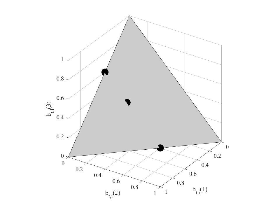
Fig.2 illustrates one example of the space reduction, where we have one node with its status update arrival rate $\lambda=0.4$. The gray triangle plane is the sub-region of $\bm{\mathcal{B}}$ in the three-dimensional space, on which each point is associated with a possible local age belief state. After the simplification, the sub-region of the belief space $\bm{\mathcal{B}}$ can be reduced to three feasible belief states, i.e., the three points plotted on the sub-region.

In [28], an RS policy was proposed to optimize the AoI of the network. In the RS policy, node $i$ is scheduled with probability $\mu_{i}\in\left(0,1\right]$ in each slot. The scheduling probabilities are time-invariant and satisfy $\sum_{i=1}^{N}\mu_{i}\leq 1$. Notice that the actions of the RS policy is independent of the network states, thus this policy can also be adopted in the considered PON. With reference to the proof of [28, Prop. 4], we give the EWSAoI performance of the RS policy, denoted by $R^{RS}$, in Proposition 3.

Note that the EWSAoI in (30) is slightly different from that in [28] due to the difference in the local age evolution of two systems. Denote by $\left\{\mu^{*}_{i}\right\}^{N}_{i=1}$ the optimal scheduling probabilities of all node, the optimal RS policy is given as follows [28, Th. 5].

According to [28, Th.10], $R^{RS*}$ is the upper bound of the EWSAoI performance of the FOMW policy, denoted by $R^{FOMW}$. The FOMW policy can be regarded as the full-observed counterpart of the POMW policy.

Built upon the proposed LOC belief-MDP, we now derive two upper bounds for the POMW policy. One of them is the EWSAoI performance of a particular RS policy, as stated in the following theorem:

Note that the value assigned to $\beta_{i}$, which depends on $\mu^{\prime}_{i}$, can be attained by minimizing the upper bound of the EWSAoI, given by $\frac{1}{N}\sum_{i=1}^{N}\omega_{i}\left(1/(\lambda_{i}\mu^{\prime}_{i}p_{i})+1\right)$. A similar method was used in [34].

Based on Theorem 2, we can analyze the performance guarantee of the POMW policy theoretically. Firstly, we introduce a universal lower bound given in [28, Th.3]. This lower bound applies to any feasible scheduling policy, and is applicable to both FONs and PONs. The universal lower bound of the EWSAoI performance of any policies is given by

References

- [1] Y. Sun and K. R. Chowdhury, “Enabling emergency communication through a cognitive radio vehicular network,” IEEE Communications Magazine, vol. 52, no. 10, pp. 68–75, 2014.
- [2] J. Wan, S. Tang, Z. Shu, D. Li, S. Wang, M. Imran, and A. V. Vasilakos, “Software-defined industrial internet of things in the context of industry 4.0,” IEEE Sensors Journal, vol. 16, no. 20, pp. 7373–7380, 2016.
- [3] R. Talak, S. Karaman, and E. Modiano, “Speed limits in autonomous vehicular networks due to communication constraints,” in 2016 IEEE 55th Conference on Decision and Control (CDC), 2016, pp. 4998–5003.
- [4] A. Kosta, N. Pappas, and V. Angelakis, “Age of information: A new concept, metric, and tool,” Foundations and Trends in Networking, vol. 12, no. 3, pp. 162–259, 2017.
- [5] M. A. Abd-Elmagid, N. Pappas, and H. S. Dhillon, “On the role of age of information in the internet of things,” IEEE Communications Magazine, vol. 57, no. 12, pp. 72–77, 2019.
- [6] X. Chen, C. Wu, T. Chen, H. Zhang, Z. Liu, Y. Zhang, and M. Bennis, “Age of information aware radio resource management in vehicular networks: A proactive deep reinforcement learning perspective,” IEEE Transactions on Wireless Communications, vol. 19, no. 4, pp. 2268–2281, 2020.
- [7] J. Liu, X. Wang, B. Bai, and H. Dai, “Age-optimal trajectory planning for uav-assisted data collection,” in IEEE INFOCOM 2018 - IEEE Conference on Computer Communications Workshops (INFOCOM WKSHPS), 2018, pp. 553–558.
- [8] M. A. Abd-Elmagid, A. Ferdowsi, H. S. Dhillon, and W. Saad, “Deep reinforcement learning for minimizing age-of-information in uav-assisted networks,” in 2019 IEEE Global Communications Conference (GLOBECOM), 2019, pp. 1–6.
- [9] R. D. Yates, “Age of information in a network of preemptive servers,” in IEEE INFOCOM 2018 - IEEE Conference on Computer Communications Workshops (INFOCOM WKSHPS), 2018, pp. 118–123.
- [10] S. Kaul, M. Gruteser, V. Rai, and J. Kenney, “Minimizing age of information in vehicular networks,” in 2011 8th Annual IEEE Communications Society Conference on Sensor, Mesh and Ad Hoc Communications and Networks, 2011, pp. 350–358.
- [11] S. Kaul, R. Yates, and M. Gruteser, “Real-time status: How often should one update?” in 2012 Proceedings IEEE INFOCOM, 2012, pp. 2731–2735.
- [12] M. Desai and A. Phadke, “Internet of things based vehicle monitoring system,” in 2017 Fourteenth International Conference on Wireless and Optical Communications Networks (WOCN), 2017, pp. 1–3.
- [13] Y. Sun, I. Kadota, R. Talak, and E. Modiano, “Age of information: A new metric for information freshness,” Synthesis Lectures on Communication Networks, vol. 12, no. 2, pp. 1–224, 2019.
- [14] B. T. Bacinoglu and E. Uysal-Biyikoglu, “Scheduling status updates to minimize age of information with an energy harvesting sensor,” in 2017 IEEE International Symposium on Information Theory (ISIT), 2017, pp. 1122–1126.
- [15] Q. Wang, H. Chen, Y. Li, Z. Pang, and B. Vucetic, “Minimizing age of information for real-time monitoring in resource-constrained industrial iot networks,” in 2019 IEEE 17th International Conference on Industrial Informatics (INDIN), vol. 1, 2019, pp. 1766–1771.
- [16] J. Pan, A. M. Bedewy, Y. Sun, and N. B. Shroff, “Minimizing age of information via scheduling over heterogeneous channels,” in Proceedings of the Twenty-Second International Symposium on Theory, Algorithmic Foundations, and Protocol Design for Mobile Networks and Mobile Computing, ser. MobiHoc ’21. New York, NY, USA: Association for Computing Machinery, 2021, p. 111–120. [Online]. Available: https://doi.org/10.1145/3466772.3467040
- [17] M. Costa, M. Codreanu, and A. Ephremides, “On the age of information in status update systems with packet management,” IEEE Transactions on Information Theory, vol. 62, no. 4, pp. 1897–1910, 2016.
- [18] Q. He, D. Yuan, and A. Ephremides, “On optimal link scheduling with min-max peak age of information in wireless systems,” in 2016 IEEE International Conference on Communications (ICC), 2016, pp. 1–7.
- [19] B. Dedhia and S. Moharir, “You snooze, you lose: Minimizing channel-aware age of information,” in 2020 18th International Symposium on Modeling and Optimization in Mobile, Ad Hoc, and Wireless Networks (WiOPT). IEEE, 2020, pp. 1–8.
- [20] Y. Sun, E. Uysal-Biyikoglu, R. D. Yates, C. E. Koksal, and N. B. Shroff, “Update or wait: How to keep your data fresh,” IEEE Transactions on Information Theory, vol. 63, no. 11, pp. 7492–7508, 2017.
- [21] S. Leng and A. Yener, “Age of information minimization for an energy harvesting cognitive radio,” IEEE Transactions on Cognitive Communications and Networking, vol. 5, no. 2, pp. 427–439, 2019.
- [22] I. Kadota, A. Sinha, and E. Modiano, “Optimizing age of information in wireless networks with throughput constraints,” in IEEE INFOCOM 2018 - IEEE Conference on Computer Communications, 2018, pp. 1844–1852.
- [23] S. Farazi, A. G. Klein, and D. R. Brown, “Average age of information for status update systems with an energy harvesting server,” in IEEE INFOCOM 2018 - IEEE Conference on Computer Communications Workshops (INFOCOM WKSHPS), 2018, pp. 112–117.
- [24] E. T. Ceran, D. Gündüz, and A. György, “Reinforcement learning to minimize age of information with an energy harvesting sensor with harq and sensing cost,” in IEEE INFOCOM 2019 - IEEE Conference on Computer Communications Workshops (INFOCOM WKSHPS), 2019, pp. 656–661.
- [25] J. P. Champati, H. Al-Zubaidy, and J. Gross, “Statistical guarantee optimization for age of information for the d/g/1 queue,” in IEEE INFOCOM 2018 - IEEE Conference on Computer Communications Workshops (INFOCOM WKSHPS), 2018, pp. 130–135.
- [26] I. Kadota, A. Sinha, E. Uysal-Biyikoglu, R. Singh, and E. Modiano, “Scheduling policies for minimizing age of information in broadcast wireless networks,” IEEE/ACM Transactions on Networking, vol. 26, no. 6, pp. 2637–2650, 2018.
- [27] J. Sun, Z. Jiang, B. Krishnamachari, S. Zhou, and Z. Niu, “Closed-form whittle’s index-enabled random access for timely status update,” IEEE Transactions on Communications, vol. 68, no. 3, pp. 1538–1551, 2020.
- [28] I. Kadota and E. Modiano, “Minimizing the age of information in wireless networks with stochastic arrivals,” IEEE Transactions on Mobile Computing, vol. 20, no. 3, pp. 1173–1185, 2021.
- [29] A. Gong, T. Zhang, H. Chen, and Y. Zhang, “Age-of-information-based scheduling in multiuser uplinks with stochastic arrivals: A pomdp approach,” in GLOBECOM 2020 - 2020 IEEE Global Communications Conference, 2020, pp. 1–6.
- [30] Y.-P. Hsu, E. Modiano, and L. Duan, “Scheduling algorithms for minimizing age of information in wireless broadcast networks with random arrivals,” IEEE Transactions on Mobile Computing, vol. 19, no. 12, pp. 2903–2915, 2020.
- [31] Z. Chen, N. Pappas, E. Björnson, and E. G. Larsson, “Age of information in a multiple access channel with heterogeneous traffic and an energy harvesting node,” in IEEE INFOCOM 2019 - IEEE Conference on Computer Communications Workshops (INFOCOM WKSHPS), 2019, pp. 662–667.
- [32] E. T. Ceran, D. Gündüz, and A. György, “A reinforcement learning approach to age of information in multi-user networks with harq,” IEEE Journal on Selected Areas in Communications, vol. 39, no. 5, pp. 1412–1426, 2021.
- [33] Q. Wang, H. Chen, C. Zhao, Y. Li, P. Popovski, and B. Vucetic, “Optimizing information freshness via multiuser scheduling with adaptive noma/oma,” IEEE Transactions on Wireless Communications, vol. 21, no. 3, pp. 1766–1778, 2022.
- [34] M. J. Neely, “Stochastic network optimization with application to communication and queueing systems,” Synthesis Lectures on Communication Networks, vol. 3, no. 1, pp. 1–211, 2010.
- [35] C. H. Papadimitriou and J. N. Tsitsiklis, “The complexity of markov decision processes,” Mathematics of operations research, vol. 12, no. 3, pp. 441–450, 1987.
- [36] G. Yao, A. M. Bedewy, and N. B. Shroff, “Age-optimal low-power status update over time-correlated fading channel,” in 2021 IEEE International Symposium on Information Theory (ISIT), 2021, pp. 2972–2977.
- [37] E. Sert, C. Sönmez, S. Baghaee, and E. Uysal-Biyikoglu, “Optimizing age of information on real-life tcp/ip connections through reinforcement learning,” in 2018 26th Signal Processing and Communications Applications Conference (SIU), 2018, pp. 1–4.
- [38] Y. Shao, Q. Cao, S. C. Liew, and H. Chen, “Partially observable minimum-age scheduling: The greedy policy,” IEEE Transactions on Communications, pp. 1–1, 2021.
- [39] D. A. McAllester and S. Singh, “Approximate planning for factored pomdps using belief state simplification,” arXiv preprint arXiv:1301.6719, 2013.
- [40] L. P. Kaelbling, M. L. Littman, and A. R. Cassandra, “Planning and acting in partially observable stochastic domains,” Artificial intelligence, vol. 101, no. 1-2, pp. 99–134, 1998.
- [41] N. L. Zhang and W. Zhang, “Speeding up the convergence of value iteration in partially observable markov decision processes,” Journal of Artificial Intelligence Research, vol. 14, pp. 29–51, 2001.
- [42] F. Chiariotti, J. Holm, A. E. Kalør, B. Soret, S. K. Jensen, T. B. Pedersen, and P. Popovski, “Query age of information: Freshness in pull-based communication,” IEEE Transactions on Communications, vol. 70, no. 3, pp. 1606–1622, 2022.
- [43] K. Liu and Q. Zhao, “Indexability of restless bandit problems and optimality of whittle index for dynamic multichannel access,” IEEE Transactions on Information Theory, vol. 56, no. 11, pp. 5547–5567, 2010.